AS-ITP-2001-005

Exclusive decay of $1^{--}$ heavy quarkonium into photon and two pions

J. P. Ma

Institute of Theoretical Physics , Academia Sinica, Beijing 100080, China

Jia-Sheng Xu

China Center of Advance Science and Technology (World Laboratory), Beijing 100080, China

and Institute of Theoretical Physics , Academia Sinica, Beijing 100080, China

Abstract

We study the exclusive decay of $1^{--}$ heavy quarkonium into one photon and two pions in the kinematic region, where the two-pion system has a invariant mass which is much smaller than the mass of heavy quarkonium. Neglecting effects suppressed by the inverse of the heavy quark mass, the decay amplitude can be factorized, in which the nonperturbative effect related to heavy quarkonium is represented by a non-relativistic QCD matrix element, and that related to the two pions is represented by a distribution amplitude of two gluons in the isoscalar pion pair. By taking the asymptotic form for the distribution amplitude and by using chiral perturbative theory we are able to obtain numerical predictions for the decay. Numerical results show that the decay of $J/\psi$ can be observed at BEPC and at CESR. Experiment observation of this process in this kinematic region at BEPC and CESR can provide information about how gluons are converted into the two pions and may supply a unique approach to study $I=0$ s-wave $\pi\pi$ scattering.
Key words: $J/\psi$ radiative decay, NRQCD, factorization, chiral perturbative theory
PACS numbers: 13.25Gv,14.40.Gx, 12.38.Bx, 12.39.Fe

Recently it has been proposed to study production of two pions in exclusive processes like $\gamma+\gamma^{*}\rightarrow\pi+\pi$[1, 2, 3] and like $\gamma^{*}+h\rightarrow h+\pi+\pi$[4, 5]. These processes will enable us to study how quarks and gluons, which are fundamental dynamical freedoms of QCD, are transmitted into the two pions. In the kinematic region, where the two pions have a much smaller invariant mass than the virtuality of the virtual photon, the scattering amplitudes of the processes take a factorized form. In this factorized form the transition of partons into the two pions are described by distribution amplitudes of partons in the two pions, which are defined with twist-2 operators. For $\gamma+\gamma^{*}\rightarrow\pi+\pi$, at the tree-level, only the distribution amplitude of quark appears in the scattering amplitude, the distribution amplitude of gluon appears at loop levels or through evolution of distribution amplitudes[1, 2, 3], while for $\gamma^{*}+h\rightarrow h+\pi+\pi$, at the tree-level, the distribution amplitude of quark as well as that of gluon contribute to the scattering amplitude, and the produced charged pion pair is in isospin $I=0$ or $I=1$ states[4, 5]. In all of the above processes, the produced system of two charged pions will be dominantly in an isospin $I\neq 0$ state. This may make it difficult to extract the distribution amplitude of gluon from experimental data, because the two pions produced through gluon conversion are in a $I=0$ state. In this letter we propose to study the radiative decay of $J/\psi$ into two pions, where the distribution amplitude of gluon appears at the tree-level and the produced two pions are dominantly in a $I=0$ state. This makes the extraction of gluon content of a two-pion system relatively easier in experiment. Beside this the decay also provides a possibility to study $I=0$ s-wave $\pi\pi$ scattering. The decay can be studied with the data sample of $5\times 10^{7}$ $J/\psi$’s whose collection will be completed with BES at the end of this year.

We consider the decay in the kinematic region where the two pions have a invariant mass which is much smaller than the mass of $J/\psi$. In the limit of $m_{c}\rightarrow\infty$ the decay amplitude can be factorized, where the nonperturbative effect of $J/\psi$ can be presented by a NRQCD matrix element, while the nonperturbative effect of the two pions is represented by the same distribution amplitude of gluon appearing in the exclusive processes mentioned above. Corrections to this limit may systematically be added. With the model for the distribution amplitude of gluon, developed in [3, 5], we obtain numerical predictions for the decay in the heavy mass limit, and they indicate that the decay is observable at BES.

We study the exclusive decay in the rest frame of $J/\psi$:

$$J/\psi(P)\rightarrow\gamma(k_{\gamma})+\pi^{+}(k_{+})+\pi^{-}(k_{-}).$$ (1)

The momenta are indicated in the brackets. We denote $k=k_{+}+k_{-}$ and $m^{2}_{\pi\pi}=k^{2}$. At leading order of QED, the S-matrix element for the decay is

$$\langle f|S|i\rangle=-iQ_{c}~{}e\int d^{4}z\langle\gamma\pi^{+}\pi^{-}|A_{\mu}(z)\bar{c}(z)\gamma^{\mu}c(z)|J/\psi\rangle,$$ (2)

where $Q_{c}$ is the electric charge of c-quark in unit of $e$, $c(z)$ is the Dirac field for c-quark. At leading order of QCD, two gluons are emitted by the c- or $\bar{c}$-quark, and these two gluons will be transmitted into the two pions. Using Wick theorem we obtain:

$$\langle f|S|i\rangle = \frac{i}{2}~{}\frac{1}{2}\delta^{ab}Q_{c}~{}e~{}g_{s}^{2}~{}\varepsilon_{\mu}^{*}(\gamma)\int d^{4}z~{}d^{4}y~{}d^{4}x~{}d^{4}x_{1}~{}d^{4}y_{1}~{}e^{i(k_{\gamma}\cdot z+k_{2}\cdot y)}$$ (3)

$$\times~{}\langle 0|\bar{c}_{j}(x_{1})c_{i}(y_{1})|J/\psi\rangle\ ~{}\langle\pi^{+}\pi^{-}|G_{\mu_{1}}^{a}(x)G_{\nu_{1}}^{b}(0)|0\rangle$$

$$\times~{}[\delta^{4}(x-x_{1})\delta^{4}(z-y_{1})\gamma^{\mu_{1}}S_{F}(x-y)\gamma^{\nu_{1}}S_{F}(y-z)\gamma^{\mu}+\cdots],$$

where $k_{2}$ is the momentum of one of emitted gluons, $S_{F}(x-y)$ is the Feynman propagator of c-quark, the dots in the square bracket denotes other five terms. In the limit of $m_{c}\rightarrow\infty$, a $c$- or $\bar{c}$-quark moves with a small velocity $v$, this fact enables us to describe nonperturbative effect related to $J/\psi$ by NRQCD, in which a systematic expansion in $v$ is employed. This expansion is extensively used for inclusive decays[6]. This expansion can also be used here for the matrix $\langle 0|\bar{c}_{j}(x_{1})c_{i}(y_{1})|J/\psi\rangle$ , in which we expand the Dirac field $c(x)$ with corresponding NRQCD fields. With the expansion we obtain:

$$\langle 0|\bar{c}_{j}(x_{1})c_{i}(y_{1})|J/\psi\rangle~{}=-\frac{1}{6}~{}(P_{+}~{}\gamma^{l}~{}P_{-})_{ij}~{}\langle 0|\chi^{\dagger}\sigma^{l}\psi|J/\psi\rangle~{}e^{-ip\cdot(x_{1}+y_{1})}+{\rm O}(v^{2}),$$ (4)

where $\chi^{\dagger}(\psi)$ is the NRQCD field for $\bar{c}(c)$ quark, $\sigma^{l}(l=1,2,3)$ is the Pauli matrix, and

$$P_{\pm} = \frac{1}{2}~{}(1\pm\gamma^{0})$$

$$p = (m_{c},0,0,0).$$ (5)

The matrix $\langle 0|\chi^{\dagger}\sigma^{l}\psi|J/\psi\rangle$ is proportional to the polarization vector $\varepsilon^{l}(J/\psi)$ at the considered order. In this paper, we neglect the contribution from higher orders in $v$, the momentum of $J/\psi$ is then approximated by $2p$. It should be noted that the effect of higher order in $v$ may be added.

Using Eq. (4) we can write the S-matrix element as

$$\langle f|S|i\rangle = \frac{-i}{24}Q_{c}~{}e~{}g_{s}^{2}~{}(2\pi)^{4}~{}\delta^{4}(2p-k-k_{\gamma})~{}\varepsilon_{\mu}^{*}(\gamma)~{}\langle 0|\chi^{\dagger}\sigma^{l}\psi|J/\psi\rangle$$ (6)

$$\int\frac{d^{4}k_{1}}{(2\pi)^{4}}H^{l\mu\mu_{1}\nu_{1}}(p,k,k_{1})~{}\Gamma_{\mu_{1}\nu_{1}}(k,k_{1}),$$

and

$$\Gamma^{\mu\nu}(k,k_{1})=\int d^{4}x~{}e^{-ik_{1}x}~{}\langle\pi^{+}\pi^{-}|G^{a,\mu}(x)G^{a,\nu}(0)|0\rangle,$$ (7)

in which $H^{l\mu\mu_{1}\nu_{1}}(p,k,k_{1})$ is a perturbative function, which is the amplitude for a $c\bar{c}$ pair emitting a photon and two gluons. The contributions in Eq.(6) can be represented by Feyman diagrams. One of them is given in Fig.1, where the kinematic variables are also indicated. The nonperturbative object $\Gamma^{\mu\nu}(k,k_{1})$ describes how two gluons are converted into $2\pi$.

Figure 1: One of the Feynman diagrams for the exclusive decay of $J/\psi$ into one photon and two pions.

In the heavy quark limit the two-pion system will have a large momentum $k$, we take a coordinate system in which the direction of $\bf k$ is the $z$-direction. For convenience we will work in the light-cone coordinate system, in which the components of $k$ are given by

$$k^{\mu}=(k^{+},k^{-},{\bf 0}),\ \ k^{+}=(k^{0}+k^{3})/\sqrt{2},\ \ k^{-}=(k^{0}-k^{3})/\sqrt{2}.$$ (8)

In the light-cone coordinate system we introduce two light cone vectors and a tensor:

$$n^{\mu} = (0,1,0,0),\ \ l^{\mu}=(1,0,0,0),$$

$$d_{T}^{\mu\nu} = g^{\mu\nu}-n^{\mu}l^{\nu}-n^{\nu}l^{\mu},$$ (9)

and we take the gauge

$$n\cdot G(x)=0.$$ (10)

The $x$-dependence of the matrix element in Eq.(7) is controlled by different scales. The $x^{-}$-dependence is controlled by $k^{+}$, which is large, while the $x^{+}-$ and ${\bf x_{T}}$-dependence are controlled by the scale $k^{-}$ and $\Lambda_{QCD}$, which are small in comparison with $k^{+}$. With this observation we can expand the matrix element in $x^{-}$ and in ${\bf x_{T}}$. At the leading order only twist-2 operators contributes to the matrix element. We will neglect higher orders in the expansion, i.e., we only keep contributions of twist-2 operators. Then we obtain:

$$\Gamma^{\mu\nu}(k,k_{1})=(2\pi)^{4}~{}\delta(k_{1}^{-})~{}\delta^{2}(k_{1T})~{}\frac{1}{k^{+}}~{}\frac{1}{x_{1}(1-x_{1})}\\ \left[\frac{1}{2}~{}d_{T}^{\mu\nu}~{}\Phi^{G}(x_{1},\zeta,m_{\pi\pi})\right],$$

with

$$\Phi^{G}(x_{1},\zeta,m_{\pi\pi}) = \frac{1}{k^{+}}~{}\int\frac{dx^{-}}{2\pi}~{}e^{-ik_{1}^{+}x^{-}}\times\langle\pi^{+}\pi^{-}|G^{a,+\mu}(x^{-}n)G^{a,+}_{\ \ \ \mu}(0)|0\rangle,$$

$$x_{1} = \frac{k_{1}\cdot n}{k\cdot n},\ \ \ \zeta=\frac{k_{+}\cdot n}{k\cdot n}.$$ (11)

$\Phi^{G}(x_{1},\zeta,m_{\pi\pi})$ is the gluonic distribution amplitude which describe how a pion pair is produced by two collinear gluons, it represents a nonperturbative effect and can only be calculated with nonperturbative methods or extracted from experiment. As it stands, it is gauge invariant in the gauge $n\cdot G(x)=0$. In other gauges we need to supply a Wilson line operator to make it gauge invariance. With Eq.(11) it is straightforward to obtain the $S$-matrix element at the tree-level in our approximation:

$$\langle f|S|i\rangle = \frac{-i}{12m_{c}^{2}}Q_{c}~{}e~{}g_{s}^{2}~{}(2\pi)^{4}~{}\delta^{4}(2p-k-k_{\gamma})\varepsilon^{*\ell}(\gamma)\langle 0|\chi^{\dagger}\sigma^{\ell}\psi|J/\psi\rangle$$ (12)

$$\int_{0}^{1}dx_{1}\frac{1}{x_{1}(1-x_{1})}\cdot\frac{8m_{c}^{2}(1-x_{1})-m_{\pi\pi}^{2}(1-2x_{1})}{4m_{c}^{2}(1-x_{1})-m_{\pi\pi}^{2}(1-2x_{1})}\cdot\Phi^{G}(x_{1},\zeta,m_{\pi\pi}).$$

In the calculation we have kept the mass $m_{\pi\pi}$. Usually the effect of $m_{\pi\pi}$ should be combined with effects of twist-4 operators as a correction to the above result. We have checked that striping the $m_{\pi\pi}$ terms changes the results by less than $5\%$. In Eq.(13) the nonperturbative effect related to $J/\psi$ and that to the two-pion system are separated, the former is represented by a NRQCD matrix element, while the later is represented by the matrix element of gluonic operators, which is defined in Eq.(12). The NRQCD matrix element is related to the wave-function of $J/\psi$ in potential models and can be estimated with these models. It can also be calculated with lattice QCD or extracted from experiment. Little is known numerically about the matrix element of gluonic operators, i.e., the function $\Phi^{G}(x_{1},\zeta,m_{\pi\pi})$. A detailed study of properties of $\Phi^{G}(x_{1},\zeta,m_{\pi\pi})$ can be found in [2, 3, 5]. For our numerical prediction we will use their results for $\Phi^{G}(x_{1},\zeta,m_{\pi\pi})$, in which asymptotic form of $\Phi^{G}(x_{1},\zeta,m_{\pi\pi})$ is taken as an Ansatz for $\Phi^{G}(x_{1},\zeta,m_{\pi\pi})$. It should be noted that the renormalization scale $\mu$ should be taken as $2m_{c}$ in our case. Because it is not very large, the actual shape of $\Phi^{G}(x_{1},\zeta,m_{\pi\pi})$ may look dramatically different than that of the asymptotic form. Keeping this in mind we take the form $\Phi^{G}(x_{1},\zeta,m_{\pi\pi})$ as that given in [5]:

$$\Phi^{G}(x_{1},\zeta,m_{\pi\pi})=-60~{}M_{2}^{G}~{}x_{1}^{2}~{}(1-x_{1})^{2}\left[\frac{3C-\beta^{2}}{12}~{}f_{0}(m_{\pi\pi})~{}P_{0}(\cos\theta_{c})\right.\\ \left.-\frac{\beta^{2}}{6}~{}f_{2}(m_{\pi\pi})~{}P_{2}(\cos\theta_{c})\right]~{},$$

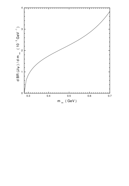
Figure 2: The differential decay branching ratio $d~{}{\rm BR}(J/\psi)/dm_{\pi\pi}$ as a function of $m_{\pi\pi}$ in unit of $10^{-3}{\rm GeV}^{-1}$.

where $\theta_{c}$ is the scattering angle of $\pi^{+}$ and $\beta$ is the velocity of $\pi^{+}$ in the center of mass system of the two pions, they are related to $\zeta$ and $m_{\pi\pi}$ by

$$\beta~{}\cos\theta_{c}=2~{}\zeta-1,~{}~{}\beta=\sqrt{1-\frac{4~{}m_{\pi}^{2}}{m_{\pi\pi}^{2}}}~{}.$$ (13)

$C$ is a constant and takes $C=1+b~{}m_{\pi}^{2}+O(m_{\pi}^{4})$ with $b\simeq-1.7{\rm GeV}^{-2}$ [3, 5], $M_{2}^{G}$ is the momentum fraction carried by gluons in the pion, its asymptotic value is

$$M_{2}^{G}=\frac{4~{}C_{F}}{N_{f}+4~{}C_{F}}.$$ (14)

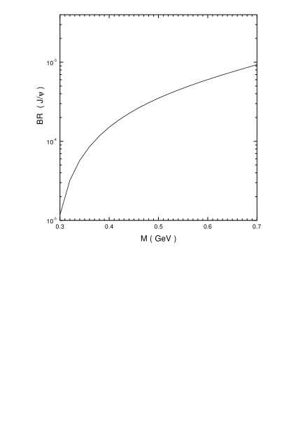
Figure 3: The decay branching ratio of $J/\psi\rightarrow\gamma+\pi^{+}\pi^{-}$ as a function of $M$, the upper cut of $m_{\pi\pi}$.

$f_{0}(m_{\pi\pi})$ and $f_{2}(m_{\pi\pi})$ are the Omnès functions for ${\rm I}=0$ S- and D-wave $\pi\pi$ scattering, respectively. The Omnès function $f_{2}(m_{\pi\pi})$ is dominated by the $f_{2}(1270)$ resonance resulting a peak at $m_{\pi\pi}=1.275{\rm GeV}$, while the Omnès function $f_{0}(m_{\pi\pi})$ in the relevant $m_{\pi\pi}$ region we studied ($m_{\pi\pi}\leq 0.70{\rm GeV}$) can be calculated by the chiral perturbative theory, the result is [7]

$$f_{0}(m_{\pi\pi})=1+\frac{m_{\pi\pi}^{2}}{192~{}\pi^{2}~{}f_{\pi}^{2}}+\frac{2m_{\pi\pi}^{2}-m_{\pi}^{2}}{32~{}\pi^{2}~{}f_{\pi}^{2}}\left[\beta~{}\ln~{}\left(\frac{1-\beta}{1+\beta}\right)+2+i\pi\beta\right],$$ (15)

where $f_{\pi}=93{\rm MeV}$is the pion decay constant.

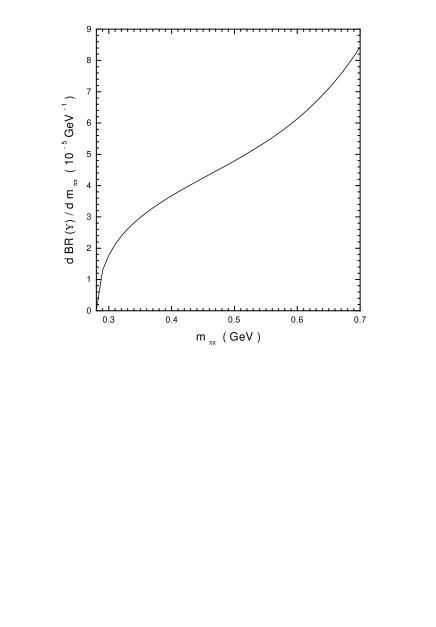
Figure 4: The differential decay branching ratio $d~{}{\rm BR}(\Upsilon)/dm_{\pi\pi}$ as a function of $m_{\pi\pi}$ in unit of $10^{-5}{\rm GeV}^{-1}$.

With these results we are able to predict the shape of the differential decay branching ratio $d~{}{\rm BR}(J/\psi)/dm_{\pi\pi}$ numerically where we use the leptonic decay of $J/\psi$ to determine the NRQCD matrix element. The result is presented in Fig.2, where we take the parameters: $m_{c}=1.5$GeV and $\alpha_{s}(2m_{c})=0.31$. We also calculate the decay branching ratio, where we use a upper cut $M$ for $m_{\pi\pi}$, hence the decay branching width is a function of $M$:

$${\rm BR}(J/\psi)=\int_{2m_{\pi}}^{M}dm_{\pi\pi}\frac{d~{}{\rm BR}(J/\psi)}{dm_{\pi\pi}}.$$ (16)

The numerical result for this decay ratio is given in Fig.3. For $M>0.38{\rm GeV}$, we can read from Fig.3 that the branching ratio is larger than $10^{-4}$, for $M=0.70{\rm GeV}$ the branching ratio is $9.3\times 10^{-4}$. Therefore it is likely that the decay mode can be measured using the data collected at BES. In the kinematic region we consider the dominant contribution to the differential decay width is from $f_{0}(m_{\pi\pi})$. The contribution from $f_{2}(m_{\pi\pi})$ is less than $10\%$. This gives a possibility to study $I=0$ s-wave $\pi\pi$ scattering in the decay. Similar results for $\Upsilon$-decay are also obtained, which are presented in Fig.4 and in Fig. 5. For $m_{\pi\pi}\leq 0.70{\rm GeV}$, the branching ratio is $2.0\times 10^{-5}$.

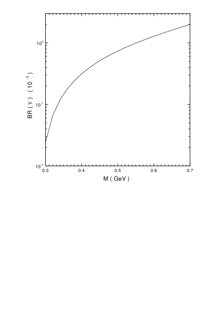
Figure 5: The decay branching ratio of $\Upsilon\rightarrow\gamma+\pi^{+}\pi^{-}$ as a function of $M$, the upper cut of $m_{\pi\pi}$ in unit of $10^{-5}$.

It should be noted that the two-pion system produced in the decay is in a S-wave state in our approximation. At twist-2 level, the produced system can also be in a D-wave state, the corresponding tensor distribution amplitude can be found in [3]. However the decay amplitude for a D-wave state is kinematically suppressed, because it is proportional to $(k_{+}-k_{-})^{\mu}(k_{+}-k_{-})^{\nu}$ and the relative momentum $(k_{+}-k_{-})$ of the two pions is a small quantity in the kinematic region considered here. If one replaces the two-pions system by the tensor meson $f_{2}(1270)$, one also finds that the decay amplitude for $f_{2}$ with the helicity $\pm 2$ is kinematically suppressed[8]. Although the effect of the D-wave state is suppressed, it can lead to some nonzero azimuthal asymmetries which may be observable in experiment.

To summarize: In this letter we have studied the exclusive decay of $1^{--}$ heavy quarkonium into one photon and two pions. At leading twist, the S-matrix of the decay takes a factorized form, the nonperturbative effect related to heavy quarkonium and that related to the light hadrons can be separated, the former is represented by a non-relativistic QCD matrix element, while the later is represented by the two-gluon to isoscalar two-pion distribution amplitude. By taking the asymptotic form for the distribution amplitude and by using chiral perturbative theory we are able to obtain numerical predictions for the decay. For $J/\psi$ , the branch ratio for $m_{\pi\pi}\leq 0.70{\rm GeV}$ is $9.3\times 10^{-4}$, while for $\Upsilon$, the branch ratio for $m_{\pi\pi}\leq 0.70{\rm GeV}$ is $2.0\times 10^{-5}$. The decay of $J/\psi$ can be studied at BES and the study can provide a possibility to study $I=0$ s-wave $\pi\pi$ scattering.

The work of J. P. Ma is supported by National Science Foundation of P. R. China and by the Hundred Young Scientist Program of Academia Sinica of P. R. China, the work of J. S. Xu is supported by the Postdoctoral Foundation of P. R. China and by The K. C. Wong Education Foundation, Hong Kong.

References

[1] M. Diehl, T. Gousset, B. Pire and O. Teryaev,
Phys. Rev. Lett. 81, 1782 (1998)
[2] M. Diehl, T. Gousset and B. Pire, Phys. Rev. D62
(2000) 073014
[3] N.Kivel, L. Mankiewicz and M. V. Polyakov, Phys. Lett.
B 467, 263 (1999)
[4] M. Polyakov, Nucl. Phys. B555 (1999) 231
[5] B. Lehmann-Dronke, A. Schaefer, M.V. Polyakov, and K. Goeke,
hep-ph/0012108
[6]G.T. Bodwin, E. Braaten, and G.P. Lepage,
Phys. Rev. D 51, 1125 (1995); Eratum:ibid.D 55,
5853 (1997)
[7] J. F. Donoghue, J. Gasser, and H. Leutwyler, Nucl. Phys.
B 343, 341 (1990)