CERN-TH/2001-017
DESY 01-027
UTHEP-01-0101

The Monte Carlo Event Generator
YFSWW3 version 1.16
for $W$-Pair Production and Decay
at LEP2/LC Energies^†

S. Jadach^a,b,c, W. Płaczek^d,c, M. Skrzypek^b,c B.F.L. Ward^e,c,f and Z. Wa̧s^b,c

^aDESY Zeuthen, Platanenallee 6, D-15738 Zeuthen, Germany
^bInstitute of Nuclear Physics, ul. Kawiory 26a, 30-055 Cracow, Poland,
^cCERN, CH-1211 Geneva 23, Switzerland,
^dInstitute of Computer Science, Jagellonian University,
ul. Nawojki 11, 30-072 Cracow, Poland,
^eDepartment of Physics and Astronomy,
The University of Tennessee, Knoxville, TN 37996-1200, USA,
^fSLAC, Stanford University, Stanford, CA 94309, USA.

We present the Monte Carlo event generator YFSWW3 version 1.16 for the process of $W$-pair production and decay in electron–positron collisions. It includes ${\cal O}(\alpha)$ electroweak radiative corrections in the $WW$ production stage together with the ${\cal O}(\alpha^{3})$ initial-state-radiation (ISR) corrections in the leading-logarithmic (LL) approximation, implemented within the Yennie–Frautschi–Suura (YFS) exclusive exponentiation framework. The photon radiation in the $W$ decays is generated by the dedicated program PHOTOS up to ${\cal O}(\alpha^{2})$ LL, normalized to the $W$ branching ratios. The program is interfaced with the $\tau$ decay library TAUOLA and the quark fragmentation/hadronization package JETSET. The semi-analytical code KorWan for the calculations of the differential and total cross-sections at the Born level and in the ISR approximation is included.

To be submitted to Computer Physics Communications

• Work partly supported by the Polish Government grant KBN 5P03B12420, the European Commission 5-th framework contract HPRN-CT-2000-00149, the US DoE Contracts DE-FG05-91ER40627 and DE-AC03-76ER00515, and the Polish–French Collaboration within IN2P3 through LAPP Annecy.

CERN-TH/2001-017
DESY 01-027
January 2001

PROGRAM SUMMARY

Title of the program: YFSWW3, version 1.16 .

Computer: any with the FORTRAN 77 compiler and the UNIX/Linux operating system

Operating system: UNIX/Linux

Programming language used: FORTRAN 77

High speed storage required: $<$ 10 MB

Size of distributed program: 3,237 kB

Distribution format: tar gzip file (size of 1,103 kB)

No. of cards in combined program and test deck: about 23,000 plus about 48,000 of auxiliary packages: KorWan, FF, JETSET, TAUOLA, PHOTOS.

Keywords:
Standard Model (SM), LEP2, linear colliders (LC), quantum electrodynamics (QED), quantum chromodynamics (QCD), boson $W$, $W$-pair production, $W$ decay, $W$ branching ratio (BR), triple gauge boson couplings (TGC), quartic gauge boson couplings (QGC), four-fermion ($4f$) background, radiative corrections, Yennie–Frautschi–Suura (YFS) exponentiation, initial-state radiation (ISR), leading-log (LL) approximation, Coulomb effect, final-state radiation (FSR), electroweak (EW) corrections, leading-pole approximation (LPA), Monte Carlo (MC) simulation/generation.

Nature of the physical problem:
The process of the $W$-pair production is important for precise tests of the Standard Model as well as searches for “new physics” at LEP2 and future linear colliders. In order to match the experimental precision necessary for a successful physics programme, quantum effects (the so-called radiative corrections) have to be included into a theoretical description of this process. It turns out that not only the so-called universal corrections (initial-state radiation, the Coulomb effect, “naive” QCD corrections, etc.) are necessary, but also the ${\cal O}(\alpha)$ electroweak corrections in the $WW$ production are needed to reach the desired theoretical accuracy. All these effects should, preferably, be included in a Monte Carlo event generator in order to account for realistic experimental set-ups.

Method of solution:
The Monte Carlo event generator for the combined $W$-pair production and decay process including ${\cal O}(\alpha^{3}$) LL ISR effects, the Coulomb correction (usual or screened), the “naive” QCD effect, the ${\cal O}(\alpha)$ EW corrections in the $WW$ production stage, implemented within the YFS exclusive exponentiation framework is provided. Multiphoton radiation in the $WW$ production is generated according to the YFS MC method. The photon radiation in the $W$ decays, normalized to the $W$ BRs, is generated by the LL-type MC program PHOTOS (up to two photons). The decays of $\tau$’s including radiative corrections are simulated by the dedicated package TAUOLA. The quark fragmentation/hadronization is performed with the help of the Lund program JETSET. The program can provide both weighted and unweighted (weight $=1$) events. Any experimental cut and apparatus efficiency may be introduced easily by rejecting some of the generated events.

Restrictions on the complexity of the problem:
The LPA is used (in two versions) to describe the signal $WW$ production process. Multiphoton radiation according to the YFS exponentiation scheme is generated only for the $WW$ production stage. ${\cal O}(\alpha)$ EW corrections (in LPA) are included only in the $WW$ production stage. The ISR effects beyond ${\cal O}(\alpha)$ are included in the LL approximation. Non-factorizable corrections (interferences between the production and decay stages) are approximated by the so-called screened Coulomb ansatz. Spin correlations between the $WW$ production and decays are fully included only at the Born and the ISR levels. Radiative corrections in the $W$ decays are included into an overall normalization through the $W$ BRs, and the real photon radiation is generated in the LL approximation (up to two photons) by the program PHOTOS. Anomalous triple gauge boson couplings are included in the Born-like matrix element, i.e. with the universal SM corrections only. Quartic gauge boson couplings are implemented according to the Standard Model only (no anomalous couplings). The $\tau$ decays and quark hadronization are performed, respectively, with the help of the dedicated packages TAUOLA and JETSET. No $4f$ background processes are included.

Typical running time:
200 CPU seconds of a PC Intel Pentium III @ 550MHz per 1000 unweighted events, for the parameter settings as they are given in the demonstration program.

1 Introduction

The process of $W$-pair production in electron–positron colliders is very important for testing the Standard Model (SM) and searching for signals of possible “new physics”; see e.g. Refs. [1, 2]. One of the main goals when investigating this process at present and future $e^{+}e^{-}$ experiments is to measure precisely the basic properties of the $W$ boson, such as its mass $M_{W}$ and width $\Gamma_{W}$. This process also allows for a study of the triple and quartic gauge boson couplings at the tree level, where small deviations from the subtle SM gauge cancellations can lead to significant effects on physical observables – these can be signals of “new physics”.

In this work we present a Monte Carlo (MC) event generator that simulates the production and decay of the $W$ pair at $e^{\pm}$ colliders. The integrated cross sections and arbitrary differential distributions can be calculated from a series of constant-weight fully inclusive MC events. The program embodies the Standard Model scattering matrix element with the ${\cal O}(\alpha$) radiative corrections for the doubly-resonant component of the scattering matrix element. The basics of the model used in the program and selected numerical results were already presented in earlier publications [3, 4, 5, 6]. The important components of the presented program/calculation are the complete ${\cal O}(\alpha$) radiative correction for on-shell $W$-pair production, which are implemented according to Refs. [7, 8, 9, 10], see also Ref. [11]. The present YFSWW3 MC event generator was instrumental in achieving the new improved theoretical precision of $0.4\%$ for the total cross section of the $WW$ production process at the highest LEP2 energies, as a result of direct and detailed comparison with the RacoonWW MC program [12, 13] within the 2000 LEP2 MC workshop (this conclusion was also supported by the comparison between RacoonWW and the calculation of Ref. [14]), see Section 4.3 in Ref. [2].

Let us briefly discuss the basic physics properties of the $W$-pair production and decay process. Since the $W$’s are unstable and short-lived particles, the $W$ pairs are not observed directly in the experiments but through their decay products: four-fermion ($4f$) final states (which may then also decay, radiate gluons/photons, hadronize, etc.). As high energy charged particles are involved in the process, one can also observe energetic radiative photons. So, at the parton level, one has to consider a general process:

$$e^{+}+e^{-}\longrightarrow 4f+n\gamma,\>\>(n=0,1,2,\ldots),$$ (1)

where also some background (non-$WW$) processes contribute. In a theoretical description of this process – according to quantum field theory – one also has to include virtual effects, the so-called loop corrections. This general process is very complicated since it involves $\sim 80$ different channels ($4f$ final states) with complex peaking behavior in multiparticle phase space and a large number of Feynman diagrams. Even in the massless-fermion approximation, the number of Feynman graphs grows up from $9$–$56$ per channel at the Born level to an enormous $3579$–$15948$ at the one-loop level [15]. The full one-loop calculations have not been finished yet, even for the simplest case (doubly plus singly $W$-resonant diagrams) [16]. But even if they existed one would be faced with problems in their numerical evaluation in practical applications, particularly within Monte Carlo event generators – they would be prohibitively huge and slow. These are the reasons why efficient approximations in the theoretical description of this process are necessary. These approximations should be such that on the one hand they would include all contributions/corrections that are necessary for the required theoretical accuracy (dependent on the experimental precision) and on the other hand they would be efficient enough for numerical computations. Given the complicated topologies of the ($4f+n\gamma$) final states, such calculations should be, preferably, given in terms of a Monte Carlo event generator that would allow one to simulate the process directly [17, 18].

Our solution to this consists of two complementary Monte Carlo event generators: YFSWW3 and KoralW. The latter includes the full lowest-order $e^{+}e^{-}\rightarrow 4f$ process, but with simplified radiative corrections – the universal ones such as initial-state radiation (ISR), the Coulomb effect, etc. In YFSWW3, on the other hand, the lowest-order process is simplified – only the doubly $W$-resonant contributions are taken into account, but inclusion of the radiative corrections in this process goes beyond the universal ones. In the current version of YFSWW3 only those non-universal (non-leading) corrections are included that are necessary to achieve the theoretical precision for the total $WW$ cross section of $0.5\%$ required for LEP2. In order to achieve a gauge-invariant description of the signal $WW$ process and to employ the existing ${\cal O}(\alpha)$ electroweak corrections for the on-shell $W$-pair production, we use the so-called leading-pole approximation (LPA). A double-pole variant of the LPA (usually referred to as DPA) was advocated in Ref. [19] and applied in a variety of calculations, see for example Refs. [12, 13, 14, 6, 20] and Ref. [2] for a review and further references. The important thing is that YFSWW3 and KoralW programs have a well established common part, which is the doubly $W$-resonant ($WW$) process with the same universal radiative corrections. This allows us to combine the results of the two programs so as to achieve the desired theoretical precision for $WW$ observables. Detailed descriptions of KoralW were published in Refs. [21, 22, 23, 24]. Here, we present a documentation of the program YFSWW3; physical aspects together with some numerical results are discussed in Refs. [3, 4, 5, 6, 20]. Possible scenarios of combining the results of the two programs are presented in Refs. [6, 20, 25].

The outline of the paper is as follows. In Section 2, we define our notation and describe the physics contents of the program. In Section 3, we discuss the MC algorithm. In Section 4, we present the structure of the program, important routines, etc. Details about the practical use of the program are given in Section 5. Finally, Section 6 summarizes the paper. Appendices contain useful technical information on the structure of the program, its input/output, etc.

2 Physics Contents of YFSWW3

In this section we describe we define differential distributions used to calculate the cross section and generate events for the $W$-pair production and decay process. These distributions we define quite completely, because they were not defined in every detail in the past publications. On the other hand we shall skip the detailed discussion of the physics models that they represent. This will be done in a separate publication [26]. First, we discuss our notation. Then we present the master formula and its ingredients. And finally, we give some details on the MC algorithms implemented in the program.

2.1 Notation

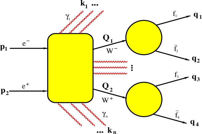
Figure 1: Kinematics of the $W$-pair production and decay process with multiple photons in the production stage.

In YFSWW3 we adopt a notational convention similar to the one used in KoralW. The variables $p_{1}$ and $p_{2}$ are the incoming $e^{-}$ and $e^{+}$ four-momenta, respectively:

$$p_{1}=(E_{e},0,0,p_{e}),\hskip 56.9055ptp_{2}=(E_{e},0,0,-p_{e}),$$ (2)

where $E_{e}$ is the beam energy and $p_{e}=\sqrt{E_{e}^{2}-m_{e}^{2}}$, with the electron mass $m_{e}$. The variables $Q_{1}$ and $Q_{2}$ are the four-momenta of the $W^{-}$ and $W^{+}$ bosons; their invariant masses are denoted by $M_{1}$ and $M_{2}$, respectively; $q_{1},q_{2}$ and $m_{1},m_{2}$ are the four-momenta and masses of the $W^{-}$ decay products; $q_{3},q_{4}$ and $m_{3},m_{4}$ are the analogous four-momenta and masses of the $W^{+}$ decay products, with the first component of each pair corresponding to a fermion and the second to an antifermion. By $k_{i}$ we denote the four-momenta of radiative photons. See also fig. 1 for a pictorial representation. The components of a four-vector are denoted by $p=(p_{0},p_{x},p_{y},p_{z})$, with the metric convention of $\{1,-1,-1,-1\}$. We also use the following Lorentz invariants: $s=(p_{1}+p_{2})^{2}$, $s_{1}=Q_{1}^{2}=M_{1}^{2}$ and $s_{2}=Q_{2}^{2}=M_{2}^{2}$.

2.2 Master Formula

Here, we consider the process:

$$e^{-}+e^{+}\longrightarrow\left\{W^{-}\rightarrow f_{1}+\bar{f}_{2}\right\}+\left\{W^{+}\rightarrow f_{3}+\bar{f}_{4}\right\}+n\gamma,\>\>(n=0,1,2,\ldots),$$ (3)

where the radiative photons are emitted only at the $WW$-production stage. The photon radiation in $W$ decays (FSR) in this version of YFSWW3 is done, in the ${\cal O}(\alpha^{2}$) leading-logarithmic (LL) approximation, by the dedicated program PHOTOS [27] – in the same way as in KoralW. Since this is done externally on fully generated events (it does not change event weights), we do not include the FSR in our discussion of the master formula. It should be remembered that the use of PHOTOS in YFSWW3 is a temporary solution before the advent of the YFS-exponentiated MC for $W$ decays.

As was already mentioned in the Introduction, we use the LPA to describe this process respecting the $SU(2)_{L}\times U(1)$ gauge invariance. In YFSWW3, we implemented two options of the LPA, called LPA_a and LPA_b. The first one, which is the default (recommended) option, is based on the approach of Stuart [19], where only the Lorentz scalar functions in the S-matrix are expanded about poles corresponding to unstable $W$’s. In the lowest order, the LPA_a matrix element coincides with the so-called CC03 (see e.g. Ref. [15] for an explanation of this notation) matrix element in the ’t Hooft–Feynman gauge. In the following we shall use the notation “CC03” in that sense. The second option, intended for some dedicated tests, follows the method suggested in Ref. [15], where the whole S-matrix residuals are expanded about poles; see Refs. [6, 20] for more details. In the following we shall describe the LPA_a scheme explicitly; LPA_b can be obtained from this by taking the $W$’s on shell (i.e. $Q_{1}^{2},Q_{2}^{2}\rightarrow M_{W}^{2}$) everywhere, except for the Breit–Wigner denominators and the phase-space integration.

In the framework of the YFS exclusive exponentiation (EEX), the cross section for the process (3) can be written as

$$\sigma_{\rm Best}= \sum_{n=0}^{\infty}\frac{1}{n!}\int\limits ds_{1}ds_{2}\frac{d^{3}Q_{1}}{Q_{1}^{0}}\frac{d^{3}Q_{2}}{Q_{2}^{0}}\prod_{l=1}^{4}\frac{d^{3}q_{l}}{q_{l}^{0}}\;\prod_{i=1}^{n}\frac{d^{3}k_{i}}{k^{0}_{i}}\;\delta^{(4)}\bigg{(}p_{1}+p_{2}-Q_{1}-Q_{2}-\sum_{i=1}^{n}k_{i}\bigg{)}$$ (4)

$$\delta^{(4)}\left(Q_{1}-q_{1}-q_{2}\right)\delta^{(4)}\left(Q_{2}-q_{3}-q_{4}\right)\;\rho^{\rm Best}_{n}(p_{1},p_{2};q_{1},\ldots,q_{4},k_{1},\ldots,k_{n}),$$

where $\rho^{\rm Best}_{n}$ is the following fully exclusive multiphoton differential distribution:

$$\rho^{\rm Best}_{n}(p_{1},p_{2};q_{1},\ldots,q_{4},k_{1},\ldots,k_{n})=\prod_{i=1}^{n}\tilde{S}(p_{1},p_{2},Q_{1},Q_{2},k_{i})\;\theta(k_{i}^{0}-k_{\epsilon})\;$$ (5)

$$\times e^{Y^{\prime}(p_{1},p_{2},Q_{1},Q_{2};k_{\epsilon})}\,\left[\,1+\delta_{C}(Q_{1},Q_{2},M_{W},\Gamma_{W})\,\right]\sum_{\wp\in\{I,W\}^{n}}p_{\wp}\,{\cal B}\left(\{p,Q,q,k\}^{{\cal R}_{\wp}}\right),$$

where ${\cal B}$ is the contribution from the infrared-finite YFS residuals:

$${\cal B} \left(\{p,Q,q,k\}^{{\cal R}_{\wp}}\right)=\left[\,1+\delta_{An}^{{\rm TGC}}\left(\{p,Q,q\}^{{\cal R}_{\wp}}\right)\,\right]\;$$ (6)

$$\times \Bigg{\{}\bar{\beta}^{(1)}_{0}\left(\{p,Q,q\}^{{\cal R}_{\wp}}\right)+\sum_{i=1}^{n}\frac{\bar{\beta}^{(1)}_{1}\left(\{p,Q,q,k_{i}\}^{{\cal R}_{\wp}}\right)}{\tilde{S}\left(\{p,Q,k_{i}\}^{{\cal R}_{\wp}}\right)}+\Delta\bar{\beta}^{(3)}_{0,{\rm ISR}}(\{p,Q,q\}^{{\cal R}_{\wp}})$$

$$+\sum_{\wp_{i}=I}\frac{\Delta\bar{\beta}^{(3)}_{1,{\rm ISR}}\left(\{p,Q,q\}^{{\cal R}_{\wp}},k_{i}\right)}{\tilde{S}_{I}(\{p\}^{{\cal R}_{\wp}},k_{i})}+\frac{1}{2!}\sum_{\wp_{i,j}=I}\frac{\bar{\beta}^{(3)}_{2,{\rm ISR}}\left(\{p,Q,q\}^{{\cal R}_{\wp}},k_{i},k_{j}\right)}{\tilde{S}_{I}(\{p\}^{{\cal R}_{\wp}},k_{i})\tilde{S}_{I}(\{p\}^{{\cal R}_{\wp}},k_{j})}$$

$$+\frac{1}{3!}\sum_{\wp_{i,j,l}=I}\frac{\bar{\beta}^{(3)}_{3,{\rm ISR}}\left(\{p,Q,q\}^{{\cal R}_{\wp}},k_{i},k_{j},k_{l}\right)}{\tilde{S}_{I}(\{p\}^{{\cal R}_{\wp}},k_{i})\tilde{S}_{I}(\{p\}^{{\cal R}_{\wp}},k_{j})\tilde{S}_{I}(\{p\}^{{\cal R}_{\wp}},k_{l})}\Bigg{\}},$$

where we use a short-hand notation of the type $\{p,Q,q\}\equiv\{p_{1},p_{2},Q_{1},Q_{2},q_{1},q_{2},q_{3},q_{4}\}$.

The sum $\sum_{\wp}$ in Eq. (5) runs over the photon partitions, i.e. all possible photon associations to the initial-state radiation (ISR) or the $W$-state radiation (WSR). For $n$ photons we identify each of the $2^{n}$ partitions ${\wp}$ with a vector ${\wp}\equiv(\wp_{1},\ldots,\wp_{n})$, where $\wp_{i}=I,W$ ($I$ and $W$ denote the ISR and the WSR photons, respectively). The partition weight $p_{\wp}$ is given by

$$p_{\wp}=\frac{\prod\limits_{\wp_{i}=I}\tilde{S}_{I}(k_{i})\prod\limits_{\wp_{j}=W}\tilde{S}_{W}(k_{j})}{\sum\limits_{\wp}\prod\limits_{\wp_{i}=I}\tilde{S}_{I}(k_{i})\prod\limits_{\wp_{j}=W}\tilde{S}_{W}(k_{j})}=\frac{\prod\limits_{\wp_{i}=I}\tilde{S}_{I}(k_{i})\prod\limits_{\wp_{j}=W}\tilde{S}_{W}(k_{j})}{\prod\limits_{i=1}^{n}\left(\tilde{S}_{I}(k_{i})+\tilde{S}_{W}(k_{i})\right)},$$ (7)

where $\tilde{S}_{I}(k)$ and $\tilde{S}_{W}(k)$ are the real photon infrared (IR) factors for the ISR and the WSR, respectively:

$$\tilde{S}_{I}(p_{1},p_{2},k)=-\frac{\alpha}{4\pi}\left(\frac{p_{1}}{kp_{1}}-\frac{p_{2}}{kp_{2}}\right)^{2},$$ (8)

$$\tilde{S}_{W}(Q_{1},Q_{2},k)=-\frac{\alpha}{4\pi}\left(\frac{Q_{1}}{kQ_{1}}-\frac{Q_{2}}{kQ_{2}}\right)^{2}.$$

It is worthwhile to stress that the partition dependence for the first two terms proportional to $\bar{\beta}^{(1)}_{0}$ and $\bar{\beta}^{(1)}_{1}$ cancels out, when truncated to ${\cal O}(\alpha$) (as it should), thanks to the special normalization choice for the partition weights: $\sum\limits_{\wp\in\{I,W\}^{n}}p_{\wp}=1$. See also the definition of $\bar{\beta}^{(1)}_{1}$ and the discussion on the partition-dependent “reduction procedure” ${\cal R_{\wp}}$ in the following. The purpose of the sum over partitions is to help the introduction of the LL corrections beyond the ${\cal O}(\alpha$).

In Eq. (6) the two components proportional to $\bar{\beta}^{(1)}_{0}$ and $\bar{\beta}^{(1)}_{1}$ explicitly represent the complete ${\cal O}(\alpha$) contribution to the $WW$-production process, while the remaining $\bar{\beta}$’s and $\Delta\bar{\beta}$’s collect the second- and third-order ISR corrections in the LL approximation; see Section 2.2.4 for more details. The dependence of the $\bar{\beta}$ functions on the photon partitions enters through the so-called reduction (extrapolation) procedures, which take into account the CMS energy shift induced by the ISR; for more details see Subsection 2.2.4.

2.2.1 YFS Infrared Factors

The real photon IR factor

$$\tilde{S}(p_{1},p_{2},Q_{1},Q_{2},k)=-\frac{\alpha}{4\pi^{2}}\left(\frac{p_{1}}{kp_{1}}-\frac{p_{2}}{kp_{2}}-\frac{Q_{1}}{kQ_{1}}+\frac{Q_{2}}{kQ_{2}}\right)^{2}$$ (9)

includes the ISR, the WSR, and the interferences between them.

The step function $\theta(k^{0}-k_{\epsilon})$, where $k_{\epsilon}=\epsilon\sqrt{s}/2$, cuts out the singular IR region, already included to all orders in the YFS form factor $e^{Y^{\prime}}$, where

$$Y^{\prime}(p_{1},p_{2},Q_{1},Q_{2};k_{\epsilon})=2\alpha\Re B^{\prime}(p_{1},p_{2},Q_{1},Q_{2})+2\alpha\tilde{B}(p_{1},p_{2},Q_{1},Q_{2};k_{\epsilon}).$$ (10)

The IR functions $\Re B^{\prime}$ and $\tilde{B}$ correspond to virtual and real photons, respectively, and are defined explicitly in Ref. [3].

2.2.2 Coulomb Correction

The correction $\delta_{C}$ is the Coulomb effect, included both (two options) in its standard form as given in Ref. [28], and in terms of the so-called screened Coulomb ansatz of Ref. [29] which is an efficient approximation of the non-factorizable corrections of Refs. [30, 31, 32, 33] for singly-inclusive distributions. It reads

$$\delta_{C}^{\rm\{Std,\,Scr\}}(Q_{1},Q_{2},M_{W},\Gamma_{W})=\frac{\alpha\pi}{2\beta}\left[1-\left\{1,\,(1-\beta)^{2}\right\}\frac{2}{\pi}\arctan\left(\frac{|\kappa|^{2}-p^{2}}{2p\Re\kappa}\right)\right],$$ (11)

with

$$\beta=\sqrt{1-2(s_{1}+s_{2})/s_{Q}+[(s_{1}-s_{2})/s_{Q}]^{2}},\;\;\;\;p=\frac{1}{2}\beta\sqrt{s_{Q}},\;\;\;\;s_{Q}=(Q_{1}+Q_{2})^{2},$$ (12)

$$\kappa=\sqrt{\frac{M_{W}}{2}\left(\sqrt{E^{2}+\Gamma_{W}^{2}}-E\right)}-i\sqrt{\frac{M_{W}}{2}\left(\sqrt{E^{2}+\Gamma_{W}^{2}}+E\right)},\;\;E=\frac{s_{Q}-4M_{W}^{2}}{4M_{W}},$$

where $M_{W}$ and $\Gamma_{W}$ are the on-shell $W$ mass and $W$ width, respectively. The first term in the curly brackets in Eq. (11) corresponds to the standard (Std) correction, the second one to the screened (Scr) Coulomb correction. This correction is properly matched with the YFS form factor, where the Coulomb-like singularity appears in the virtual IR function $\Re B$. After matching it with the full Coulomb correction $\delta_{C}$, the original YFS function $\Re B$ is replaced by $\Re B^{\prime}$, as described in Ref. [3].

2.2.3 Anomalous Triple-Gauge Couplings

The anomalous corrections to the triple-gauge couplings (TGC) $WWV$ ($V=Z$,$\gamma$) are included multiplicatively through

$$1+\delta_{An}^{{\rm TGC}}=\frac{|{\cal M}_{{\rm Born}}^{An{\rm TGC}}|^{2}}{|{\cal M}_{{\rm Born}}^{\rm SM}|^{2}},$$ (13)

where ${\cal M}_{{\rm Born}}^{An{\rm TGC}}$ is the Born-level matrix element with the anomalous TGCs, while ${\cal M}_{{\rm Born}}^{\rm SM}$ is the corresponding SM matrix element. In YFSWW3 we use the same conventions (routines) for the TGCs as they are given in KoralW [23]. The anomalous couplings are included in the event generation only if an appropriate switch in the input parameters is on and the parameters corresponding to these couplings (in a given parameterization) are set up to non-SM values; see Appendix A for details.

2.2.4 $\bar{\beta}$’s for $W$-Pair Production

In the IR-finite $\bar{\beta}$ functions of Eq. (5), we see the superscripts ${\cal R}_{\wp}$ in the four-momenta arguments like $\{p,Q,q\}^{{\cal R}_{\wp}}$ or $\{p,Q,q,k\}^{{\cal R}_{\wp}}$. This means that these arguments are subject to the “reduction (extrapolation) procedures”. These reduction procedures are partition-dependent – this is why they are denoted with the subscripts $\wp$. The partition dependence enters through accounting for the ISR energy shift $s\rightarrow s^{\prime}$, where $s^{\prime}=(p_{1}+p_{2}-\sum_{\wp_{i}=I}k_{i})^{2}$ in the evaluation of the $\bar{\beta}$ functions. For more discussion on the meaning of the reduction/extrapolation procedures, see Subsection  2.3. In YFSWW3, we use the reduction procedures of the YFS2 and YFS3 programs of KORALZ [34, 35, 36], with some modifications: in constructing the reduced $W$ four-momenta, we take into account that, in general, $M_{1}\neq M_{2}$. We perform appropriate transformations of the $W^{\pm}$ decay products, that is we boost them to $W$’s rest frames before the reduction, and then make the inverse boost transformation to the reduced frame. In general, the effect (recoil) of the CMS energy shift $s\rightarrow s^{\prime}$ is taken due to the ISR photons only. This procedure is well justified for the ISR corrections beyond ${\cal O}(\alpha$) where we take $\{p,Q,q\}^{{\cal R}_{\wp}}$ and for each photon we may say whether it belongs to the ISR or to the WSR. For the ${\cal O}(\alpha$) specific corrections we cannot make a distinction, in the corresponding $\bar{\beta}$’s, between the ISR and the WSR; the $\{p,Q,q,k_{i}\}^{{\cal R}_{\wp}}$ in their arguments means that (i) the reduced $\{p,Q,k_{i}\}^{{\cal R}_{\wp}}$ are within the 3-body phase space and (ii) the photon $k_{i}$ is excluded from the energy shift $s\rightarrow s^{\prime}$ calculation. For more discussion on this non-trivial point see Subsections 2.3 and 2.4.

Let us now describe in detail the ${\cal O}(\alpha$)-complete functions $\bar{\beta}^{(1)}_{0}$ and $\bar{\beta}^{(1)}_{1}$. The first one, which includes the ${\cal O}(\alpha)$ electroweak (EW) virtual corrections, reads as follows:

$$\bar{\beta}^{(1)}_{0}(\{p,Q\})=\bar{\beta}^{(0)}_{0}(\{p,Q\})\left[1+\delta^{(1)}_{v+s}(\{p,Q\};k_{\epsilon})-Y(\{p,Q\};k_{\epsilon})\right],$$ (14)

where $\bar{\beta}^{(0)}_{0}$ is the lowest-order matrix element squared for the $W$-pair production and decay; it is identical to the corresponding $\bar{\beta}^{(0)}_{0}$ function in KoralW [21, 23]. In fact, the $\bar{\beta}^{(1)}_{0}$ function comes in two variants. The first one, referred to as scheme (A) [6], reads as follows:

$$\bar{\beta}^{(1)}_{0,A}(\{p,Q\}) =\bar{\beta}^{(0)}(\{p,Q\})\,\left[1+\delta^{(1)}_{\rm ISR}(p_{1},p_{2})\right]$$ (15)

$$+\bar{\beta}^{(0)}(\{p,Q\})\bigg{[}\delta^{(1)}_{v+s}(\{p,Q\};k_{\epsilon})-Y(\{p,Q\};k_{\epsilon})-\delta^{(1)}_{\rm ISR}(p_{1}^{\rm eff},p_{2}^{\rm eff})\bigg{]}_{G_{\mu}}$$

where $\delta^{(1)}_{\rm ISR}=(\alpha/\pi)[\ln(s/m_{e}^{2})-1]$ is the LL pure QED ${\cal O}(\alpha)$ ISR correction, and the subscript $G_{\mu}$ means that the whole correction is calculated in the so-called $G_{\mu}$ scheme [7] as explained in Ref. [6]. Another option, referred to as scheme (B), similar to the one used in the program RacoonWW [13], is defined as follows:

$$\bar{\beta}^{(1)}_{0,B} (\{p,Q\})=\bar{\beta}^{(0)}(\{p,Q\})\,\left[1+\delta^{(1)}_{\rm ISR}(p_{1},p_{2})\right]$$ (16)

$$+\bar{\beta}^{(0)}(\{p,Q\})\bigg{[}\delta^{(1)}_{v+s}(\{p,Q\};k_{\epsilon})-Y(\{p,Q\};k_{\epsilon})-\delta^{(1)}_{\rm ISR}(p_{1}^{\rm eff},p_{2}^{\rm eff})\bigg{]}_{G_{\mu}}\left(\frac{\alpha}{\alpha_{G_{\mu}}}\right),$$

where $\alpha$ is the fine structure constant and $\alpha_{G_{\mu}}=(\sqrt{2}G_{\mu}M_{W}^{2}\sin^{2}\theta_{W})/\pi$. Here, although the ${\cal O}(\alpha)$ corrections are calculated in the $G_{\mu}$ scheme, their relative coefficient is $\alpha$ instead of $\alpha_{G_{\mu}}$. Our recommended option is scheme (A), which is inspired by the renormalization group equations (RGEs) [37, 6].

The ${\cal O}(\alpha)$ virtual and soft photon corrections for the $WW$ production stage are included in $\delta^{(1)}_{v+s}$. In the current version of the program, we use the calculations of Ref. [7] for the on-shell $WW$-production. Since in our case the $W$’s are off-shell, we have to perform some transformations/extrapolations in order to employ these calculations. We do it in the following way. After performing the reduction procedure for the $\bar{\beta}_{0}$ function, as described above, we find $\cos\theta_{\rm eff}$ and the velocity $\beta_{\rm eff}$ of the $W$’s in the reduced frame, where

$$\beta_{\rm eff}=\sqrt{1-2(s_{1}+s_{2})/s^{\prime}+[(s_{1}-s_{2})/s^{\prime}]^{2}},$$ (17)

$$\cos\theta_{\rm eff}=(\vec{p}_{1}^{{\cal R}_{\wp}}\cdot\vec{Q}_{1}^{{\cal R}_{\wp}})/(|\vec{p}_{1}^{{\cal R}_{\wp}}||\vec{Q}_{1}^{{\cal R}_{\wp}}|).$$

Then, for this value of $\beta_{\rm eff}$ we calculate the effective CMS energy squared for on-shell $W$’s:

$$s_{\rm eff}=4M_{W}^{2}/(1-\beta_{\rm eff}^{2}).$$ (18)

Having ($s_{\rm eff}$, $\beta_{\rm eff}$, $\cos\theta_{\rm eff}$), we construct the four-momenta $(p_{1}^{\rm eff},p_{2}^{\rm eff},Q_{1}^{\rm eff},Q_{2}^{\rm eff})$ for the on-shell process $e^{+}e^{-}\rightarrow W^{+}W^{-}$ and use them to calculate the respective EW corrections. The same four-momenta are used to calculate the IR form factor $Y$ according to Eq. (10); now the Coulomb-like singularity in the virtual IR function $\Re B$ is kept, in order to cancel the corresponding singularity in $\delta^{(1)}_{v+s}$, and to calculate the ${\cal O}(\alpha)$ ISR correction:

$$\delta^{(1)}_{\rm ISR}(p_{1}^{\rm eff},p_{2}^{\rm eff})=\frac{\alpha}{\pi}\left(\ln\frac{s_{\rm eff}}{m_{e}^{2}}-1\right).$$ (19)

Such a procedure allows us to use the EW corrections also in the $WW$-threshold region, however, in this region the LPA becomes less precise. Since there exists no other calculation with the ${\cal O}(\alpha)$ EW corrections for the $W$-pair production and decay process in the $WW$-threshold region, we estimate, for the moment, the precision of YFSWW3 in that region at $2\%$ conservatively, just as for the ISR approximation. This can be improved in the future, when more calculations/tests are done.

Two comments are in order about the approximations used in the evaluation of Eqs. (14–16):

1. In the LPA_a,b, the one-loop corrections should be evaluated “on-pole”, i.e. for the complex $W$ mass: $M^{2}=M_{W}^{2}-iM_{W}\Gamma_{W}$. This would, however, require the analytic continuation of the on-shell one-loop corrections to the second Riemann sheet. We avoid this by using the approximation $M\simeq M_{W}$ in the LPA residuals. Since this is done for the ${\cal O}(\alpha)$ corrections, the error introduced by this approximation is of the order of $(\alpha/\pi)(\Gamma_{W}/M_{W})<10^{-4}$, which is negligible for the precision we aim at.

2. A coherent sum over $W$ spins between the production and decay stages is included in Eq. (14) in the $\bar{\beta}_{0}^{(0)}$ function, but not in the non-leading (NL) ${\cal O}(\alpha)$ EW correction. This should be sufficient for the LEP2 precision as the total EW correction in the LEP2 energy range is typically $\sim 1$–$2\%$. However, the $W$-spin effects can be included also in the NL ${\cal O}(\alpha)$ EW correction, if necessary.

The ${\cal O}(\alpha)$ real photon ISR and photon emission in the $WW$-production stage are included through the following IR-finite function:

$$\bar{\beta}^{(1)}_{1}\left(\{p,Q,q,k\}^{{\cal R}_{\wp}}\right) =D_{\gamma}^{(1)}\left(\{p,Q,q,k\}^{{\cal R}_{\wp}}\right)-\tilde{S}\left(\{p,Q,q,k\}^{{\cal R}_{\wp}}\right)\,\bar{\beta}_{0}^{(0)}\left(\{p,Q,q\}^{{\cal R}_{\wp}}\right),$$ (20)

where $D_{\gamma}^{(1)}$ is the differential cross section for the single hard photon radiation in the $WW$-production stage and the non-radiative $W$-decays. For this we use the calculations of Ref. [8], where the $W$’s are taken on shell. In order to accommodate them in our off-shell process, we use general formulae for $W$-polarization vectors in terms of their off-shell four-momenta [38] in the spin amplitude calculations, and perform a coherent summation over the $W$’s polarizations of the production and decay amplitudes. In fact, the hard-photon amplitudes of Ref. [8] are given in the massless-fermion approximation, so they become inaccurate when a photon is emitted close to a fermion direction. To correct this, we supplement these amplitudes with the mass terms according to the CALKUL prescription of Ref. [39].

In Eqs. (4) and (5) we use the IR-finite $\bar{\beta}$ functions for the ISR $\bar{\beta}_{0,{\rm ISR}}^{(3)}$, $\bar{\beta}_{1,{\rm ISR}}^{(3)}$, $\bar{\beta}_{2,{\rm ISR}}^{(3)}$ and $\bar{\beta}_{3,{\rm ISR}}^{(3)}$, calculated up to ${\cal O}(\alpha^{3}$) LL. They are exactly the same as in KoralW, see Ref. [23]. We define in addition:

$$\Delta\bar{\beta}_{0,{\rm ISR}}^{(3)}=\bar{\beta}_{0,{\rm ISR}}^{(3)}-\bar{\beta}_{0,{\rm ISR}}^{(1)},\quad\Delta\bar{\beta}_{1,{\rm ISR}}^{(3)}=\bar{\beta}_{1,{\rm ISR}}^{(3)}-\bar{\beta}_{1,{\rm ISR}}^{(1)}.$$ (21)

In Eqs. (4) and (5), they are evaluated only for the ISR photons. In principle, these ISR residuals could be calculated for all photons – it is still consistent with the LL ISR approximation.

2.2.5 Pretabulated EW Corrections

We have implemented also the pretabulated (or “fast”) version of the EW corrections. In this mode, a pretabulation of the NL ${\cal O}(\alpha)$ EW corrections

$$\delta_{\rm EW}^{\rm NL}(\{p,Q\})=\delta^{(1)}_{v+s}(\{p,Q\};k_{\epsilon})-Y(\{p,Q\};k_{\epsilon})-\delta^{(1)}_{\rm ISR}(p_{1},p_{2})$$ (22)

is done in the initialization stage of the program. Then, during the event generation, a linear interpolation of the pretabulated values is performed for each event. The pretabulation is done as a function of $\cos\theta$ of the $W^{-}$ for fixed values of the CMS energy $\sqrt{s}$ (set-up to the nominal energy) and of the $W$ invariant masses (set-up to $M_{W}$). This means, that in this approach, the ISR energy shift $s\to s^{\prime}$ as well as the off-shellness of the $W$’s is not taken into account (the latter prevents this method from being used below the $WW$-threshold). In that respect, the pretabulated version of the EW corrections should be regarded as some approximation of the YFSWW3 “best” prediction. The main advantage of this version is that it is much faster in computing time than the exact (“best”) one, because here the time-consuming EW library is invoked only at the beginning of the program run for some number of equally spaced points instead of by calling it for each generated event. We have checked that at $\sqrt{s}=200$ GeV, the results for the total cross section and main distributions of the pretabulated version differ from the corresponding results of the “best” one by only $0.1\%$, which is well below the required theoretical precision for the LEP2 data analysis.

2.2.6 Fixed-Order Calculation

By truncating the master formula (4) at some power of the coupling constant $\alpha$, one can obtain a fixed-order calculation, e.g. ${\cal O}(\alpha^{0}$), ${\cal O}(\alpha^{1}$).

At ${\cal O}(\alpha^{0}$) (the Born approximation), one gets the differential distribution

$$\rho_{0}^{(0)}(\{p,Q,q\})=\bar{\beta}_{0}^{(0)}(\{p,Q,q\}).$$ (23)

At ${\cal O}(\alpha^{1}$), there are two contributions: (1) from the one-loop virtual corrections and the real soft photon radiation

$$\rho_{0}^{(1)}(\{p,Q,q\};k_{\epsilon})=\bar{\beta}_{0}^{(0)}(\{p,Q,q\})\left[1+\delta^{(1)}_{v+s}(\{p,Q\};k_{\epsilon})\right],$$ (24)

and (2) from the real hard photon radiation

$$\rho_{1}^{(1)}(\{p,Q,q\},k)=D_{\gamma}^{(1)}(\{p,Q,q\},k).$$ (25)

We have implemented the above fixed-order calculations in YFSWW3. They are available through the parallel weights, as explained in Table 9 of Appendix A. For $\delta^{(1)}_{v+s}$ we use the calculation of Ref. [7], and for $D_{\gamma}^{(1)}$ the calculation of Ref. [8]; see also Subsection 2.2.4 for more details.

2.2.7 Radiative Corrections for $W$ Decays

Radiative corrections in $W$ decays are not included in the above formulae explicitly. However, we include them in the overall normalization of the cross section by normalizing the $W$ decay amplitudes to the $W$ branching ratios (BR), which can be provided through the input parameters of the program. This means that in the $\bar{\beta}$ functions of Eq. (6) for the $(i,j)$-th $W^{-}W^{+}$ decay channel, we use the normalization constant

$${\cal N}_{ij}=\frac{B_{i}B_{j}}{B_{ref}^{2}},$$ (26)

with

$$B_{ref}=\frac{\alpha_{W}M_{W}}{12\Gamma_{W}\sin^{2}\theta_{W}},$$ (27)

where $\theta_{W}$ is the weak mixing angle, and $\alpha_{W}=\alpha_{G_{\mu}}$ in our recommended $G_{\mu}$ scheme, while we set $\alpha_{W}=\alpha$ in the so-called $\alpha$ scheme. $B_{i}$ is the BR for the $i$-th $W$-decay channel, while $B_{ref}$ is the reference BR used for the normalization of the actual matrix element; see Ref. [21] for more details. For the fully inclusive process (all channels), the normalization constant is

$${\cal N}_{all}=\frac{1}{B_{ref}^{2}}.$$ (28)

It turns out that the BRs calculated at the Born level in the $G_{\mu}$ scheme – the so-called improved Born approximation (IBA) – agree within $0.1\%$ with the full one-loop results [15]. Such an IBA option is also included in the program – for this one needs only to supply (through the input parameters) the values of the CKM matrix elements. In that case

$$B_{i}=\left\{\begin{array}[]{l}B_{ref}:\hskip 136.57323pt{\rm for\>\;leptons,}\\ 3\,|V_{i}^{\rm CKM}|^{2}\left(1+\frac{\alpha_{s}(M_{W}^{2})}{\pi}\right)B_{ref}:\hskip 11.38109pt{\rm for\>\;quarks,}\end{array}\right.$$ (29)

where $V_{i}^{\rm CKM}$ is the CKM matrix element for the $i$-th $W$-decay channel, and $\alpha_{s}(M_{W}^{2})$ is the QCD coupling constant at the $M_{W}$ scale.

By construction, the real photon radiation in $W$ decays, which is generated by PHOTOS, does not affect the overall normalization of the cross section – this is of course motivated by the KLN theorem [40, 41].

2.2.8 ISR Reference Differential Distribution

Equations (4) and (5) define the so-called “best” physics model of YFSWW3; if the corresponding weight is used as a rejection weight in order to generate unweighted (constant-weight) events, then we say that YFSWW3 is run in the “best” mode. We want to combine the fully exclusive (multiphoton) differential distributions from YFSWW3 and KoralW, so that the resulting distributions contain both the LPA ${\cal O}(\alpha)$ EW corrections (missing in KoralW) and $4f$-background diagram corrections (missing in YFSWW3), using event-per-event correction weights. In order to do this, we must define a certain simplified, auxiliary, fully exclusive, differential distribution $d\sigma_{R}$, which is common to both programs, and implement the corresponding MC weight $w_{R}$ in both programs. In YFSWW3 the weight $w_{R}$ can be used also optionally, as a main rejection weight – this is the so-called “ISR mode”. Otherwise, $w_{R}$ is one of many alternative weights calculated simultaneously with the “best model weight”; it is available to the user, and/or it is used to calculate the correction weight that serves the purpose of introducing the missing ${\cal O}(\alpha)$ EW corrections in events generated by KoralW.

In the reference distribution $d\sigma_{R}$, only the numerically leading corrections, i.e. the ISR, the Coulomb correction, etc., are taken into account. This reference distribution includes the CC03 matrix element defined identically in YFSWW3 and KoralW. We also say, sometimes, that this is the distribution of the ISR-type model. The corresponding fully exclusive, reference, differential distribution, replacing $\rho_{n}$ of Eq. (5), we define as follows:

$$\rho^{R}_{n}(p_{1},p_{2};q_{1},\ldots,q_{4},k_{1},\ldots,k_{n})=\prod_{i=1}^{n}\tilde{S}_{I}(p_{1},p_{2},k_{i})\;\theta(k_{i}^{0}-k_{\epsilon})\;$$ (30)

$$\times e^{Y_{I}(p_{1},p_{2};\epsilon)}\;\left[\,1+\delta_{C}(Q_{1},Q_{2},M_{W},\Gamma_{W})\,\right]\left[\,1+\delta_{An}^{{\rm TGC}}\left(\{p,Q,q\}^{{\cal R}}\right)\,\right]\;$$

$$\Bigg{\{}\bar{\beta}^{(3)}_{0,{\rm ISR}}\left(\{p,Q,q\}^{{\cal R}}\right)+\sum_{i=1}^{n}\frac{\bar{\beta}^{(3)}_{1,{\rm ISR}}\left(\{p,Q,q\}^{{\cal R}},k_{i}\right)}{\tilde{S}_{I}\left(\{p\}^{{\cal R}},k_{i}\right)}+\sum_{i>j}^{n}\frac{\bar{\beta}^{(3)}_{2,{\rm ISR}}\left(\{p,Q,q\}^{{\cal R}},k_{i},k_{j}\right)}{\tilde{S}_{I}(\{p\}^{{\cal R}},k_{i})\tilde{S}_{I}(\{p\}^{{\cal R}},k_{j})}$$

$$+\sum_{i>j>l}^{n}\frac{\bar{\beta}^{(3)}_{3,{\rm ISR}}\left(\{p,Q,q\}^{{\cal R}},k_{i},k_{j},k_{l}\right)}{\tilde{S}_{I}(\{p\}^{{\cal R}},k_{i})\tilde{S}_{I}(\{p\}^{{\cal R}},k_{j})\tilde{S}_{I}(\{p\}^{{\cal R}},k_{l})}\Bigg{\}},$$

where we have made the following replacements with respect to Eq. (5):

$$Y^{\prime}\;\longrightarrow\;Y_{I}(p_{1},p_{2};\epsilon)=2\frac{\alpha}{\pi}\left[\left(\ln\frac{s}{m_{e}^{2}}-1\right)\ln\epsilon+\frac{1}{2}\ln\frac{s}{m_{e}^{2}}-1+\frac{\pi^{2}}{2}\right],$$ (31)

$$\tilde{S}\;\longrightarrow\;\tilde{S}_{I}(p_{1},p_{2},k),$$

and we include the pure ISR LL $\bar{\beta}$’s only. The WSR is just absent from the above distribution, which means that there is only one photon partition (where all photons are associated to the ISR) with the weight $p_{\wp}=1$. In the actual MC program, $\rho^{R}_{n}$ should be implemented with a MC weight in the operational mode when the WSR is switched off – through the parallel weights. Both of these possibilities are included in YFSWW3. However, it can also be implemented as a MC weight when the WSR is switched on. In such a case, the sums over the $\bar{\beta}$’s should extend to all photons.

The above ISR reference cross section is also used in this and other works to define the so-called non-leading (NL) corrections

$$\sigma_{\rm NL}\equiv\sigma-\sigma_{R}=\int\left(d\sigma-d\sigma_{R}\right).$$ (32)

The subscript NL expresses the fact that these corrections are numerically smaller than the leading ISR corrections. It does not mean, however, that these corrections are free of logarithmic contributions, such as $\ln(s/M_{W}^{2})$, but these logarithms are numerically much smaller than the ISR basic logarithm $\ln(s/m_{e}^{2})$.

As already indicated, the reference ISR differential distribution of Eq. (30) (for the same CC03 matrix element) is also implemented in KoralW, and it has been checked numerically to a very high accuracy [6, 25] that its KoralW implementation agrees with that of the present YFSWW3 program. Having done that, it is possible to combine the results of the KoralW and YFSWW3 programs by reweighting the MC events, in order to include both the effects of the $4f$ background and the LPA ${\cal O}(\alpha)$ NL corrections in the MC predictions for the $W$-pair production and decay process. This is done in practice by reweighting the MC events produced by KoralW with the correction weight provided by YFSWW3. The correction $\delta^{R}_{\rm NL}$ to be used by KoralW is defined as

$$1+\delta^{R}_{\rm NL}=\frac{\rho^{\rm Best}_{n}(p_{1},p_{2};q_{1},\ldots,q_{4},k_{1},\ldots,k_{n})}{\rho^{R}_{n}(p_{1},p_{2};q_{1},\ldots,q_{4},k_{1},\ldots,k_{n})},$$ (33)

where the numerator and denominators are defined in Eqs. (5) and (30). A few remarks are in due order. The above ratio is, in fact, calculated as the ratio of the corresponding MC weights. The YFSWW3 program has to be run in the mode with the WSR switched on, because $\rho^{\rm Best}_{n}$ includes the summation over the ISR–WSR photon partitions, see Eq. (5), through the multichannel reduction procedure ${\cal R}_{\wp}$. Under these conditions the above correction includes the complete ${\cal O}(\alpha)$ correction, which can be used to correct the fully exclusive distributions generated by KoralW, on an event-per-event basis. As we shall see in Subsection 4.12, the YFSWW3 program provides at present only a numerically efficient approximation of the above $\delta^{R}_{\rm NL}$.

2.3 YFS Reduction/Extrapolation Procedures

It is characteristic and inherent feature of the YFS exponentiation that the IR-finite $\bar{\beta}_{i}$ distributions require extrapolation to a larger phase space with the additional “spectator” photons. For instance, the function $\bar{\beta}_{0}$ is in our case originally defined at the $(\{q_{1},q_{2},q_{3},q_{4}\})=(\{q\})$ point of the 4-particle phase space and it has to be also defined at every $(\{q\},k_{1},\ldots,k_{n})$ point of the ($4+n$)-particle phase space. We call the procedure of extending the domain of the $\bar{\beta}_{0}$ function $\bar{\beta}_{0}(\{q\})\to\bar{\beta}^{E}_{0}(\{q\},k_{1},\ldots,k_{n})$ the “extrapolation procedure”. The only true limitation in the choice of the extrapolation procedure is that $\bar{\beta}^{E}_{0}(\{q\},0,\ldots,0)=\bar{\beta}_{0}(\{q\})$ must hold. Typically, $\bar{\beta}_{0}(\{q\})$ is defined in terms of dot-products of the four-momenta $p_{i}\cdot q_{j}$ (or inner spinor products). Extrapolation may be done in a natural way by using exactly the same algebraic expressions in the larger phase space as were originally obtained from the Feynman diagrams in the smaller phase space. In the smaller phase space, the dot products obey certain relations due to the four-momentum conservation, which no longer hold true in the presence of the additional photons – this is the main mechanism in the realization of such an extrapolation. Another useful method of implementing the extrapolation (especially in the case when $\bar{\beta}_{0}(\{q\})$ is implemented in the form of a black-box procedure, which requires as the input the four-momenta in the 4-particle phase space) is to project the $(\{q\},k_{1},\ldots,k_{n})$ point into the “reduced” point $\{q\}^{{\cal R}}$ using some kinematical manipulations (boosts, rotations, rescalings) on the four-momenta, and subsequently plugging it into $\bar{\beta}^{E}_{0}(\{q\},k_{1},\ldots,k_{n})\equiv\bar{\beta}_{0}(\{q\}^{{\cal R}})$. The above “reduction procedure” is, of course, less general than the extrapolation procedure. Last, but not least, let us note that the extrapolation procedure $(\{q\})\to(\{q\},k_{1},\ldots,k_{n})$ is the reverse procedure to that of defining the residua at the IR-divergent points/poles $(\{q\},k_{1},\ldots,k_{n})\to(\{q\})=(\{q\},0,\ldots,0)$ in the derivation of the resummation of the IR divergences to the infinite order (i.e. the derivation of the YFS exponentiation). The extrapolation procedure $\bar{\beta}_{1}(\{q\},k_{j})\to\bar{\beta}^{E}_{1}(\{q\},k_{1},\ldots,k_{j},\ldots,k_{n})$ is quite analogous. It has to obey the relation $\bar{\beta}_{1}(\{q\},k_{j})\to\bar{\beta}^{E}_{1}(\{q\},0,\ldots,0,k_{j},0,\ldots,0)$. Here all photons except the $j$-th one are the spectators.

It should be stressed that the above freedom, due to a reduction/extrapolation procedure, is a well-known feature of the YFS exponentiation, already underlined in Ref. [42] and discussed in many works implementing the YFS exponentiation; see for example Refs. [34, 43]. The uncertainty of the results due to the reduction/extrapolation procedure in the ${\cal O}(\alpha^{n}$) YFS-exponentiated calculation is always at least of ${\cal O}(\alpha^{n+1}$); it does not influence or spoil the ${\cal O}(\alpha^{n}$) perturbative “exact” contributions coming from the ${\cal O}(\alpha^{n}$) Feynman-diagram calculations. On the contrary, a reasonable choice of the reduction/extrapolation procedure may improve significantly the total precision, because the YFS exponentiation is then able to sum up efficiently higher-order effects beyond the “exact” ${\cal O}(\alpha^{n}$), as was often seen [44, 45, 46, 47]. The above remark is also valid for the special “multichannel” variant of the reduction/extrapolation procedure described in the following.

2.4 Multichannel YFS Reduction/Extrapolation

It is useful sometimes to split the $\bar{\beta}$’s into several components and introduce a different extrapolation/reduction procedure for each component. This is perfectly within the limits of our freedom. For instance in YFS3, in the centre of mass of the $Z$-boson, neither the initial beams nor the final fermion pairs have the momenta back-to-back. There are four possible definitions of the scattering angles in this frame. One defines $\bar{\beta}_{0}$ as a sum of four differential Born-level distributions, each for a different scattering angle. They might be summed up with the same weight 1/4, but, in fact, also a more sophisticated mixture is implemented [48]. A similar multichannel extrapolation procedure is used in BHLUMI [43, 45]. In the present work, we employ another kind of multichannel extrapolation, introduced for the first time in the unpublished program BHWIDE [46].

Let us elaborate on that method. Our exponentiation model is based on the real soft photon factor $\tilde{S}$ and the corresponding virtual photon function $\Re B$ to which photons emitted from the beams and from the $W$’s contribute coherently. We cannot, therefore, say whether a given photon is emitted from the initial state or from the $W$’s. We may, however, say something about it in a probabilistic way. If we split $\tilde{S}$ as follows:

$$\tilde{S}(k)=-\frac{\alpha}{4\pi^{2}}\left(\frac{p_{1}}{kp_{1}}-\frac{p_{2}}{kp_{2}}-\frac{Q_{1}}{kQ_{1}}+\frac{Q_{2}}{kQ_{2}}\right)^{2}=\tilde{S}_{I}(k)+\tilde{S}_{W}(k)+\tilde{S}_{int}(k),$$ (34)

$$\tilde{S}_{I}(k)=\left(\frac{p_{1}}{kp_{1}}-\frac{p_{2}}{kp_{2}}\right)^{2},\quad\tilde{S}_{W}(k)=\left(\frac{Q_{1}}{kQ_{1}}-\frac{Q_{2}}{kQ_{2}}\right)^{2}\quad$$

we may define for each photon a probability

$$p_{I}(k)=\frac{\tilde{S}_{I}(k)}{\tilde{S}_{I}(k)+\tilde{S}_{W}(k)}$$ (35)

that it was emitted from the beams, and the probability $p_{W}(k)=1-p_{I}(k)$ that it was emitted from the $W$’s. The above probabilities are a kind of LL concept, which has to be used with care. It may help to sum up higher-order QED corrections in the LL approximation. In particular, it may allow us to construct a multichannel type of reduction/extrapolation in which we may say for the spectator photons whether they were emitted by the beams (ISR) or by the $W$ bosons (WSR). This is done as follows: for each phase-space point we split the differential distributions into $2^{n}$ components, corresponding to $2^{n}$ possible associations of $n$ photons to the ISR or the WSR, the weight being the product $P(k)$ of the corresponding $p_{I}(k_{i})$ or $p_{W}(k_{i})$. This product is exactly the partition weight $p_{\wp}$ in Eqs. (4) and (7). For each component we may apply a separate reduction procedure which “knows” whether a given spectator photon belongs to the ISR or the WSR. The above procedure is, in practice, simpler than is said above, because in the MC realization we start from the YFS3 differential distribution, in which $\tilde{S}_{int}(k)$ is neglected, and the sum over the associations of photons to the ISR or the WSR is “randomized”. In other words, we generate only one of the $2^{n}$ possible associations and therefore, for a given event, we work with only one component (association), for which we may immediately employ its “native” reduction procedure – that is we may use the information on the photon associations directly from the YFS3 MC generator; see also the next section for an additional discussion. Let us stress again that this powerful solution should be used with care, especially for the non-spectator photons in the $\bar{\beta}$ functions.

3 Monte Carlo Algorithm

In constructing the MC algorithm for the cross-section calculation and the event generation, we start from the master formula of Eq. (4) and perform step-by-step simplifications in the differential distribution, compensating them with appropriate weights. We do this until we reach a simple enough differential distribution to be generated using the standard MC techniques. The MC algorithm of YFSWW3 for the Born-like $WW$ production and decay is identical to the one used in KoralW for the so-called CC03 option [21], while the algorithm for the multiphoton radiation in the $e^{+}e^{-}\rightarrow W^{+}W^{-}$ process is based on the one implemented in the program YFS3 of KORALZ [36] for the process $e^{+}e^{-}\rightarrow f\bar{f}$. Since $W$’s are much heavier than light fermions and, in general, have different invariant masses, we had to make a few modifications in the latter algorithm. The most important of them are:

• generalization of the photon radiation formulae to allow for large and different masses of radiating particles,

• inclusion of interferences between the radiation from the initial state and that from the $WW$ state, both in the YFS IR functions $\tilde{S}$ and $Y$ and in the IR-finite residuals $\bar{\beta}$.

The algorithm of YFS3, although used for a decade as part of other programs, was not documented until recently. Its first full description can be found in two recent works [48, 47]. We therefore do not describe it here in detail, but refer the interested reader to the above two papers. We explain below only the main steps in the YFSWW3 algorithm that lead to the algorithms of YFS3 and KoralW, and then comment on the YFS reduction/extrapolation procedures.

3.1 Main Steps in the Construction of the MC Weight

The MC algorithm of YFSWW3 is based on the importance-sampling method. In constructing it, we start from the master formula (4) and make a series of simplifications compensating them with appropriate weights until we reach a distribution that is simple enough to be generated using the basic MC methods (see e.g. Refs. [49, 50]), as we indicated above. Here, we describe only the main simplifications in Eq. (4) that lead to the formula that can be generated with the help of the MC algorithms used in the programs YFS3 and KoralW. They are:

1. $\bar{\beta}$ functions:
   For the aggregate of the $\bar{\beta}$ functions we do the following replacement:

   $${\cal B}\left(\{p,Q,q,k\}^{{\cal R}_{\wp}}\right)\longrightarrow b_{0}\left(\{p,Q,q\}^{{\cal R}_{\wp}}\right),$$ (36)

   which is compensated by the “model” weight

   $$w_{\beta}^{\wp}=\frac{{\cal B}\left(\{p,Q,q,k\}^{{\cal R}_{\wp}}\right)}{b_{0}\left(\{p,Q,q\}^{{\cal R}_{\wp}}\right)},$$ (37)

   where $b_{0}=\bar{\beta}_{0}^{(0)}$ is the Born-level differential cross section for the $W$-pair production and decay process as given in Eq. (4) of Ref. [21]. To evaluate the model weight $w_{\beta}^{\wp}$, we use the partition-dependent reduction procedures described in Subsection 2.2.4.

2. YFS form factor:
   We simplify this with the replacement:

   $$Y^{\prime}(p_{1},p_{2},Q_{1},Q_{2};k_{\epsilon})\longrightarrow Y_{I}(p_{1},p_{2};\epsilon)+Y_{W}(Q_{1},Q_{2};k_{\epsilon}),$$ (38)

   which is compensated by the weight

   $$w_{Y}=\exp[Y^{\prime}-Y_{I}-Y_{W}],$$ (39)

   where $Y_{I}$ is given in Eq. (31) and $Y_{W}$ is the YFS IR function corresponding to the photon radiation from the $W^{-}W^{+}$ electric dipole:

   $$Y_{W}(Q_{1},Q_{2};k_{\epsilon})=2\alpha\Re B(Q_{1},Q_{2})+2\alpha\tilde{B}(Q_{1},Q_{2},k_{\epsilon}).$$ (40)

   The explicit formulae for the above $\Re B$ and $\tilde{B}$ are given in Ref. [3]; we do not repeat them here because they are rather lengthy. This simplification corresponds to neglecting the ISR–WSR interference terms in the YFS form factor.

3. $\tilde{S}$ factors:
   In these we also neglect the ISR–WSR interferences:

   $$\tilde{S}(p_{1},p_{2},Q_{1},Q_{2},k)\longrightarrow\tilde{S}_{I}(p_{1},p_{2},k)+\tilde{S}_{W}(Q_{1},Q_{2},k),$$ (41)

   and compensate this by the weight

   $$w_{\tilde{S}}=\prod_{i=1}^{n}\frac{\tilde{S}(p_{1},p_{2},Q_{1},Q_{2},k)}{\tilde{S}_{I}(p_{1},p_{2},k)+\tilde{S}_{W}(Q_{1},Q_{2},k)},$$ (42)

   where $\tilde{S}_{I}$ and $\tilde{S}_{W}$ are given in Eq. (8).

After these simplifications, we obtain from Eq. (4) the formula for the first-level, “crude” cross section:

$$\sigma_{\rm Crude}= \sum_{n=0}^{\infty}\frac{1}{n!}\int\limits ds_{1}ds_{2}\frac{d^{3}Q_{1}}{Q_{1}^{0}}\frac{d^{3}Q_{2}}{Q_{2}^{0}}\prod_{l=1}^{4}\frac{d^{3}q_{l}}{q_{l}^{0}}\;\left[\prod_{i=1}^{n}\frac{d^{3}k_{i}}{k^{0}_{i}}\left\{\tilde{S}_{I}(k_{i})+\tilde{S}_{W}(k_{i})\right\}\,\theta(k_{i}^{0}-k_{\epsilon})\right]$$ (43)

$$\delta^{(4)}\left(p_{1}+p_{2}-Q_{1}-Q_{2}-\sum_{i=1}^{n}k_{i}\right)\delta^{(4)}\left(Q_{1}-q_{1}-q_{2}\right)\delta^{(4)}\left(Q_{2}-q_{3}-q_{4}\right)$$

$$e^{Y_{I}+Y_{W}}\sum\limits_{\wp\in\{I,W\}^{n}}p_{\wp}\,b_{0}\left(\{p,Q,q\}^{{\cal R}_{\wp}}\right).$$

The above distribution can be generated using the MC algorithms of YFS3 and KoralW. To make this more transparent, we shall write this formula in a slightly different but equivalent form.

The product of the $\tilde{S}$-factors in the square brackets of Eq. (43) together with the sum over the photon partition can be written as

$$\prod_{i=1}^{n}\frac{d^{3}k_{i}}{k^{0}_{i}}\left\{\tilde{S}_{I}(k_{i})+\tilde{S}_{W}(k_{i})\right\}\,\theta(k_{i}^{0}-k_{\epsilon})\sum\limits_{\wp\in\{I,W\}^{n}}p_{\wp}\,b_{0}\left(\{p,Q,q\}^{{\cal R}_{\wp}}\right)=$$ (44)

$$\sum_{\wp\in\{I,W\}^{n}}\;\prod_{\wp_{i}=I}\frac{d^{3}k_{i}}{k^{0}_{i}}\tilde{S}_{I}(k_{i})\theta(k_{i}^{0}-k_{\epsilon})\prod_{\wp_{j}=W}\frac{d^{3}k_{j}}{k^{0}_{j}}\tilde{S}_{W}(k_{j})\theta(k_{j}^{0}-k_{\epsilon})\,b_{0}\left(\{p,Q,q\}^{{\cal R}_{\wp}}\right),$$

where we have substituted Eq. (7) for the partition weight $p_{\wp}$.

After some algebra, and exploiting the Bose–Einstein symmetry for photons, the formula of Eq. (43) can be written as

$$\sigma_{\rm Crude}= \sum_{n_{I}=0}^{\infty}\sum_{n_{W}=0}^{\infty}\int\limits ds^{\prime}\frac{d^{3}P^{\prime}}{{P^{\prime}}^{0}}\,\delta^{(4)}\left(p_{1}+p_{2}-\sum_{i=1}^{n_{I}}k_{i}-P^{\prime}\right)ds_{1}ds_{2}\frac{d^{3}Q_{1}}{Q_{1}^{0}}\frac{d^{3}Q_{2}}{Q_{2}^{0}}\,$$ (45)

$$\left[\frac{1}{n_{I}!}\prod_{i=1}^{n_{I}}\frac{d^{3}k_{i}}{k^{0}_{i}}\tilde{S}_{I}(k_{i})\,\theta(k_{i}^{0}-k_{\epsilon})\right]\left[\frac{1}{n_{W}!}\prod_{j=1}^{n_{W}}\frac{d^{3}k_{j}}{k^{0}_{j}}\tilde{S}_{W}(k_{j})\,\theta(k_{j}^{0}-k_{\epsilon})\right]$$

$$\delta^{(4)}\left(P^{\prime}-Q_{1}-Q_{2}-\sum_{j=1}^{n_{W}}k_{j}\right)\prod_{l=1}^{4}\frac{d^{3}q_{l}}{q_{l}^{0}}\,\delta^{(4)}\left(Q_{1}-q_{1}-q_{2}\right)\delta^{(4)}\left(Q_{2}-q_{3}-q_{4}\right)\,$$

$$e^{Y_{I}}e^{Y_{W}}\,b_{0}\left(\{p,Q,q\}^{{\cal R}_{\wp}}\right),$$

where $s^{\prime}={P^{\prime}}^{2}$ is the CMS energy squared in the ISR-reduced (effective) frame, and $n_{I}$ and $n_{W}$ are the multiplicities of the ISR and WSR photons, respectively.

To generate the ISR and WSR according to Eq. (45), we can use the MC algorithm of YFS3 (see Refs. [48, 47]) for multiphoton radiation in the fermion-pair production, where the initial-final-state interferences were neglected. The only modification we had to do in this algorithm was to extend it to the case of heavy particles of unequal masses (see Ref. [48]). Generating particular values of $n_{I}$ and $n_{W}$ corresponds to choosing a given photon partition for $n=n_{I}+n_{W}$ in the sum of Eq. (44). This means that the sum over partitions is “randomized” in the program, i.e. not evaluated directly but generated using the MC methods. For the given (generated) photon partition, we then calculate the weights $w_{\beta}^{\wp}$, $w_{Y}$ and $w_{\tilde{S}}$. Such a solution can be regarded as a multibranch MC algorithm, see Ref. [50], where each branch corresponds to a particular photon partition.

3.2 MC Weights and Absolute Normalization

In the process of simplifying the fully differential distribution of Eq. (4)

$$\sigma_{\rm Best}=\sum_{n=0}^{\infty}\frac{1}{n!}\int d{\rm Lips}_{n}(\{p;q\},k_{1},\ldots,k_{n})\rho^{\rm Best}_{n}(\{p;q\},k_{1},\ldots,k_{n})$$ (46)

described in the previous section we have finished with the “crude differential distribution” $\rho^{\rm Crude}$ inside the integral

$$\sigma_{\rm Crude}=\sum_{n_{I}=0}^{\infty}\sum_{n_{W}=0}^{\infty}\frac{1}{n_{I}!}\frac{1}{n_{W}!}\int d{\rm Lips}_{n}(\{p;q\},k_{1},\ldots,k_{n})\;\rho^{\rm Crude}_{n_{I},n_{W}}(\{p;q\},k_{1},\dots,k_{n}),$$ (47)

where $n=n_{I}+n_{W}$. Using the above notation, the total correcting weight is defined as follows:

$$w^{(1)}=\frac{\rho^{\rm Best}_{n}(\{p;q\},k_{1},\ldots,k_{n})}{\rho^{\rm Crude}_{n_{I},n_{W}}(\{p;q\},k_{1},\dots,k_{n})}=w_{\beta}^{\wp}\;w_{Y}\;w_{\tilde{S}}.$$ (48)

In the actual program it comes in several versions, because for the purpose of the technical tests, and for the discussion of the physical precision, we need to switch off/on certain contributions in the full distribution $\rho^{\rm Best}_{n}$.

However, in the actual MC program we do not actually generate the distribution $\rho^{\rm Crude}$, but a certain, more primitive, “primary” distribution $\rho^{\rm Prim}$. For its definition and full description, and the description of how events are generated according to this distribution, starting from the uniform random numbers, we refer the reader to the most complete documentation of the YFS3 Monte Carlo algorithm in Ref. [48]; Refs. [21] and [34] can also be helpful. The weight correcting for the transition from the primary to crude distribution is given by

$$w^{(2)}=\frac{\rho^{\rm Crude}_{n_{I},n_{W}}(\{p;q\},k_{1},\ldots,k_{n})}{\rho^{\rm Prim}_{n_{I},n_{W}}(\{p;q\},k_{1},\ldots,k_{n})}$$ (49)

and is fully defined in Ref. [48]. The total MC weight is of course equal to the product

$$w=w^{(1)}\;w^{(2)}$$ (50)

or

$$w=w^{\rm Model}\;w^{\rm Crude},$$ (51)

with

$$w^{\rm Model}=w_{\beta}^{\wp}\;b_{0},\hskip 28.45274ptw^{\rm Crude}=w^{(2)}\,w_{Y}\,w_{\tilde{S}}\;b_{0}^{-1},$$ (52)

where $w^{\rm Model}$ is called in the program the “model weight” (this weight and its many variants are provided in the WtSet array; see Section 5), and $w^{\rm Crude}$ is called the “crude weight” (in the program it is equal to the product WtCrud1*WtCrud2; see Section 5).

The integrated cross section is given by the product of the average weight and the integrated primary cross section

$$\sigma=\langle w\rangle\,\sigma^{\rm Prim}=\langle w\rangle\int d\sigma^{\rm Prim}.$$ (53)

The integrated primary cross section we also call a “normalization cross section”, because it provides the absolute normalization for the whole MC calculation.

4 Structure of the Program

In this section we provide the reader with a brief guide of the YFSWW3 program. We shall describe its main routines, libraries and interfaces. We want to note here that the program, in the distribution version, is prepared for a UNIX/Linux-type operating system that supports directories and the make utility. The source code is distributed over a number of subdirectories, in order to make the structure of the program more transparent and easier to handle. Also a system of the Makefile’s is provided, for compilation, execution and other auxiliary functions (e.g. clean-up). (Of course, this organization, which is in fact rather simple, can be avoided and the whole source code can be put into a single FORTRAN file.) In the following we give a review of all YFSWW3 subdirectories. We start from the directories that are most interesting from the user’s point of view, then going to the ones with more technical contents. In the distribution package, all these subdirectories are located in the main YFSWW3 directory: yfsww3-1.16-export. This directory also comprises two important files: README and RELEASE.NOTES, which we recommend the user look through before using the program. They contain some basic information about YFSWW3: how to compile/link and run the program, a brief documentation of the code, etc.

4.1 demo – Demonstration Program

The subdirectory demo contains a demonstration program in the file demo.f. Generally, the user is supposed to provide his/her own main program; nevertheless, the file quoted here provides a simple example of such a program. It has a double role: (1) as a useful template, and (2) as a first cross-check that the MC generator YFSWW3 runs correctly on a given installation. The essential part of this program is a loop in which a series of MC events is generated. It also reads the input from a disk file, but no histogramming is performed and most of the output comes from the generator itself. At the end of the program, a MC-integrated cross section of YFSWW3 is compared with the Born-level and ISR results from the semi-analytical program KorWan. The program is compiled/linked and executed, with the help of Makefile, for the input data set given in the files demo.input. The program also reads the default settings provided in the file data_DEFAULTS located in the directory data_files – some of these default settings are overridden by data from demo.input. The demonstration program is run for unweighted events with the external libraries PHOTOS, TAUOLA and JETSET switched on. The output, written into the disk file demo.output, can then be compared with the one provided in the file demo.output.linux. It was obtained on a PC Intel Pentium III under the Linux RedHat 6.1 operating system.

4.2 data_files – Default Input Data

The subdirectory data_files contains the input data file data_DEFAULTS, which gives the defaults settings for YFSWW3. It is identical with the one used in the program KoralW, so the two programs can be set-up from the same input data file! This considerably facilitates a combination the results of the two programs; see Ref. [25] for more details. Some entries in this data file are dummy for YFSWW3 and are kept only for compatibility with KoralW, while some of them are specific to YFSWW3 and are treated as dummy parameters in KoralW. They are accompanied by appropriate comments. This file can also be used as a template to create the user’s own input data file, where only those entries that will have different settings from the default data file may be included. The user input file should be read after the file data_DEFAULTS, so that the user settings can override the default ones; see the example in the demo.f file described in the previous subsection. This directory comprises also some older data files kept for backward compatibility. Their names contain, after a dot, the last two digits of the year of their creation. (The latest of these files is identical with the file data_DEFAULTS.)

4.3 yfsww – Master Unit

The subdirectory yfsww contains the actual Monte Carlo event generator. Subprograms that can be used directly are the following:

• YFSWW_ReaDataX – the subprogram used to read, from the disk file, the default input data of YFSWW3 and subsequently the data of the user into the array xpar at the very beginning of the use of YFSWW3.

• YFSWW_Initialize – the subprogram that does all initializations of internal variables. First, it sets-up the main parameters of the program (through the routine filexp) according to the values in the input data files, then it calls several initializers of the main internal modules of the generator, such as KarLud(-1,...), and of external packages, such as TAUOLA, etc. It prints out directly or indirectly all the input parameters.

• YFSWW_Make – the most important subprogram of YFSWW3. It generates single MC events. Functionally, it is a high-level management subprogram in the event generation. It invokes (through the routine yfsww3) other routines that perform specific tasks, such as: generation of ISR photons (KarLud), generation of radiative photons from $W$’s (KarFin), generation of the $W$’s and final $4f$ four-momenta (WW_Presam), evaluation of the Coulomb correction (WTCoul), calculation of the matrix element (Model), of the YFS form factor, of the interference corrections, etc. It builds up the total MC weight from the weights supplied by these routines. This weight is then returned, in the weighted-event mode, as the main event weight, or used in the rejection loop (in the routine yfsww3), in the unweighted-event mode, for constructing the weight $=1$ event. It also calls PHOTOS, which generates photon radiation in the $W$ decays, TAUOLA for decaying of the final-state $\tau$’s (if they appear), and JETSET to perform fragmentation/hadronization of the final-state quarks. It keeps track, through special monitoring routines, of all the information necessary for the final results from the MC event generation.

• YFSWW_Finalize does all final bookkeeping, including the calculation of the integrated (total) cross section. It prints a summary output for the whole sample of generated MC events.

The first subprogram is located in the file readata.f, while the following three are in the file yfsww3.f.

This directory contains also a collection of utility routines, which can be used, for instance, to access information on particle flavours and four-momenta, on event weights, etc. They are located in the file ww_get.f (see the comments in this file for more details).

4.4 model – Matrix Elements

The routines for the “model” weights calculations are located in the subdirectory model. The master routine here is the subroutine Model (in the file model.f); by calling some other routines, this evaluates the “model” weights $w^{\rm Model}$ as defined in Eq. (52).

1. For the Born-level matrix element we use the same routines as in the program KoralW – they are collected in the file born.f. The same again are used for the ISR corrections, located in the file betas.f.

2. The ${\cal O}(\alpha)$ virtual and real soft photon corrections are evaluated with the help of a special interface – the routine VirSof – in the file virsof.f. In the first call, this routine makes all the necessary initializations, and then calculates the EW corrections by calling appropriate routines from the EW library for each generated event. The pretabulated (or “fast”) version of the EW correction is invoked through the routine DnlFast (in the file dnlfast.f). This routine makes a pretabulation of the EW corrections in the initialization stage of the program and then, during the event generation, it performs the linear interpolation of the pretabulated values to calculate the EW corrections for each event as described in Section 2.2.5.

3. The ${\cal O}(\alpha)$ hard photon matrix element in the $WW$ production, which contributes to the function $\bar{\beta}_{1}$, see Eq. (20), is calculated with the help of the routine eewwg, located in the file eewwg.f. This routines evaluates appropriate spin amplitudes for the process $e^{+}e^{-}\rightarrow W^{+}W^{-}\gamma$ according to the formulas of Ref. [8], which are then combined coherently with the spin amplitudes for $W$ decays.

In order to calculate all these contributions to the $\bar{\beta}$ functions, the subroutine Model calls the routines that perform appropriate “reduction” procedures as described in Section 2. Except for calculating the contributions to the YFS exponentiated cross section, this routine provides also the weights corresponding to the strict ${\cal O}(\alpha^{0}$) and ${\cal O}(\alpha^{1}$) calculations. In the end, the subroutine Model fills the array of weights with the weights corresponding to: (i) several variants of the SM models (for example different orders of QED ISR) and (ii) various components in the differential cross section for a given variant of the SM (for example contributions from various $\bar{\beta}$’s). The subroutine Model returns the best “model” weight.

The routine WTCoul – in the file coulco.f – for the Coulomb (both “standard” and “screened”) correction calculation is also located in this directory.

4.5 ewc – Electroweak Library

The subdirectory ewc contains the routines for the calculation of the electroweak (virtual plus soft photon) corrections in the on shell $WW$ production process according to Refs. [7, 11]. For the evaluation of one-loop integrals they use the package FF of Ref. [51], which is located in a separate directory (see below).

4.6 interfs – Interfaces to External Libraries

Interfaces to some external libraries are collected in the directory interfs. The most important routines are:

• inietc – in the file tauola_photos_ini.f – sets up some parameters of PHOTOS and TAUOLA.

• tohep – in the file hepface.f – fills in the /HEPEVT/ COMMON block, calls PHOTOS for photon radiation in $W$ decays and TAUOLA for $\tau$ decays.

• tohad – in the file lundface.f – calls JETSET for the quark fragmentation/hadronization.

Note that the COMMON block /HEPEVT/ is expected to contain single-precision (REAL*4) variables.

4.7 wdeclib – External Libraries for $W$ Decay

The subdirectory wdeclib provides the following programs:

• PHOTOS [27] for photon radiation in the $W$ decays (up to two photons),

• TAUOLA [52] for $\tau$ decays with radiative corrections,

• JETSET version 7.4 [53] for quark fragmentation/hadronization,

located in the files: photos.f, tauola.f and jetset74.f, respectively.

In YFSWW3 1.16 we use the recently modified PHOTOS, where also the photon radiation from quarks can be activated with the help of a special input parameter switch; see the tables with the input parameters in Appendix A. Note that in the distribution version of TAUOLA the parameters in the $\tau$-decay modes are not adjusted to the recent experimental data. We recommend the user to replace this version of TAUOLA with the one accepted within his/her own collaboration. The technical update described in Refs. [54, 55] will resolve this inconvenience in the future releases of the program.

4.8 glib – Histogramming and Numerical Library

A handy FORTRAN histogramming package, GlibK [56], is provided in the subdirectory glib (the file glibk.f). It is used by YFSWW3 both for hard-coded internal bookkeeping and for some optional “external” tests. The package is similar in its usage to the classic HBOOK of CERNLIB. This subdirectory also contains the useful numerical package yfslib.f with the routines for weight monitoring, random-number generation, numerical integration, one- and two-dimensional adaptive MC sampling, Lorentz transformations, etc.

4.9 semian – Semi-Analytical Program KorWan

The subdirectory semian contains the package KorWan for the semi-analytical calculations of the cross section for the off-shell $WW$ production and decay at the Born level and with the ISR corrections (using the structure-function formalism). Also the Coulomb effect is included in KorWan in both versions: the “standard” and the “screened” ones. The package is described in detail in Refs. [21, 22, 23]. It can be used for a quick consistency check of the YFSWW3 results.

4.10 ff – FF Package

In the subdirectory ff is located the FF package [51] for the evaluation of one-loop integrals needed to calculate the ${\cal O}(\alpha)$ EW virtual corrections.

4.11 dok – Related Papers

In the subdirectory dok, we include some of our papers related to YFSWW3. They are in the form of gzip’ed PostScript files.

4.12 rewt – Reweighting Tools

The subdirectory rewt contains routines that are not needed for the standard MC event generation but for various event reweighting purposes. We provide here the tools for two kinds of reweighting: the reweighting (1) of the KoralW generated events to correct for ${\cal O}(\alpha)$ NL effects in $WW$ production, and (2) of the YFSWW3 generated events to take into account effects due to some input parameters (typicaly $W$-mass) changes. All these tools are described in detail in the following; see also the file README provided in this subdirectory.

4.12.1 Reweighting KoralW Events by YFSWW3

The main tool for this kind of reweighting is the function YFSWW_WtNL, located in the file rewt_K.f. For the events, in terms of flavours and four-momenta of the final-state fermions and the ISR photons, provided through its parameters, this function calculates and returns the corresponding correction weight from YFSWW3. This weight is a ratio of the fully differential distribution. In practice, we calculate the ratio of the MC weights corresponding to two distributions – this is more convenient. We can do it because the common crude distribution entering both weights cancels out, for a given number of real photons of Eq. (5), to the reference distribution in the “ISR approximation” defined in Eq. (30), which is the same as in KoralW in the CC03 mode (Eq. (4) of Ref. [23]). It is defined in Eq. (33). In the reweighting mode of YFSWW3, we implement an approximate version of this weight:

$$w^{-}_{\rm NL}\equiv\frac{\rho_{n}^{{\rm Best}-}(\{p,Q,q\}^{{\cal R}_{I}},k_{1},\ldots,k_{n})}{\rho_{n}^{R}(\{p,Q,q\}^{{\cal R}_{I}},k_{1},\ldots,k_{n})}=1+\delta^{R}_{\rm NL-},$$ (54)

where $\rho^{{\rm Best}-}_{n}$ is a variant of $\rho^{{\rm Best}}_{n}$ in which the sum over the photon partitions is reduced to only one term, in which all photons are associated to the ISR with the partition probability $p_{\wp}=1$, and ${\cal R}_{I}$ means the respective reduction procedure. Unfortunately, we loose in this way a (small) part of the genuine ${\cal O}(\alpha)$ corrections. The full ${\cal O}(\alpha)$ correction can be included only if YFSWW3 is run in the event-generation mode, and the correction weight for reweighting (accounting for the $4f$ background) is supplied from KoralW. (This leads, however, to large MC weight fluctuations, see below.) We have checked, however, that the bias introduced in the LEP2 energy range by this approximation is within $0.1\%$, both for the total cross section and for distributions. This can be explained by the fact that the $W$’s, as heavy and slowly moving particles, do not radiate much at these energies. Of course, the main weight of YFSWW3 based on $\rho^{{\rm Best}}_{n}$ does not have this bias. In this way, by assigning this correction weight to the KoralW events, one can include, in a simple way, the ${\cal O}(\alpha)$ NL correction $\delta^{R}_{\rm NL-}$ into the KoralW results. How to do it in practice, we explain in detail in Ref. [25].

4.12.2 Reweighting YFSWW3 Events by YFSWW3

This kind of reweighting can be useful in some data analyzes, e.g. when one has accumulated a large sample of simulated events for a given input parameter set-up and one wants to assess the effects of changing some of the input parameters, but without having to repeat the full simulation with the new input parameters. The tools for such a reweighting are collected in the file rewt_Y.f. We provide two methods: “exact” and “approximate”. In the exact method the partition vector for photons is stored along with their four-momenta, while in the approximate method the partition information is not recorded.

(a) The exact method:

The tool for the exact method is SUBROUTINE YFSWW_WME(WtME), where WtME corresponds to the weight $w^{\rm Model}$ of Eq. (52). It requires storing on the disk/tape the entire content of four COMMON blocks: /MOMINI/, /MOMFIN/, /MOMDEC/ and /DeChan/ during the event-generation run of YFSWW3. We assume that the appropriate tools for writing the above information on the disk/tape as well as for reading it in the reweighting run of the program are provided by the user of the code (see the source code for more details).

How to use it:

1. The primary-run generating/storing events:
   $\bullet$ Run YFSWW3 and store on the disk/tape the whole content of the COMMON blocks:     /MOMINI/, /MOMFIN/, /MOMDEC/, /DeChan/.
       This is done for some input parameters set-up (A).

2. The secondary-run reweighting events:
   $\bullet$ Initialize the program with the input parameters set-up (A) used for the event       generation.
   $\bullet$ Instead of generating events, call YFSWW_WME(WtME_A) for all stored events and       save the computed matrix element weight WtME_A (in some arbitrary units).
   $\bullet$ Initialize the program with a different input parameters set-up (B).
   $\bullet$ Calculate the weight WtME_B and save as above.
   $\bullet$ For each event, calculate the ratio Wt = WtME_B/WtME_A and use it as the weight     for reweighting the original sample of events.
   $\bullet$ This procedure can be repeated for any new input parameters set-up (B).

Example of running the program in the reweighting mode:

 CALL YFSWW_ReaDataX(’./data_DEFAULTS’,1,10000,xpar)  ! reading general defaults
 CALL YFSWW_ReaDataX(’./user.input’   ,0,10000,xpar)  ! reading user input
 CALL YFSWW_Initialize(xpar)                          ! initialize generator
 NevTot = 1000            ! number of events to be reweighted
 DO Iev = 1, NevTot
    CALL YFSWW_WME(WtME)  ! calculate matrix element weight for stored events
 ENDDO

For more information about running YFSWW3, see Section 5.

(b) The approximate (simpler) version:

In the case when one does not have all the information needed for the exact (recommended) method of reweighting (because of the lack of disk/tape space or some other reasons), one can use

     WtME = YFSWW_WME_Smpl(Iflav,pf1,pf2,pf3,pf4,Phot,Nphot)

instead of CALL YFSWW_WME(WtME). In this case one needs to store for each event only the flavours and four-momenta of the final-state fermions and the number and the four-momenta of all photons. Important: They should come from YFSWW3 itself, not from PHOTOS after the FSR. These four-momenta and flavours are available from two COMMON blocks:

     COMMON / DECAYS / Iflav(4),amdec(4)
     COMMON / MOMDEC / pf1(4),pf2(4),pf3(4),pf4(4),Phot(100,4),Nphot

(the fermion mass array amdec(4) does not need to be stored). They can be alternatively accessed with the help of two getter-routines:

     SUBROUTINE YFSWW_Get4f(flav,p1,p2,p3,p4)
     SUBROUTINE YFSWW_GetPhotAll(NphAll,PhoAll)

located in the file ww_get.f in the subdirectory yfsww. The first one provides the flavours and four-momenta of the final-state 4-fermions, while the second one provides the number and four-momenta of the radiative photons (excluding the ones from PHOTOS).

The FUNCTION YFSWW_WME_Smpl fills the appropriate COMMON blocks and calculates (returns) the matrix element weight (corresponding to WtME in the previous method). This method is approximate because it does not use the information on the photon partitions but assigns all the photons to the ISR in performing the partition-dependent reduction procedure (described in Section 2.2). Our tests show, however, that the differences between this and the exact method are numerically negligible, e.g. $<0.01\%$ for the total cross section at $\sqrt{s}=200$ GeV.

4.12.3 Reweighting YFSWW3 Events by KoralW

Similar reweighting tools are provided in the new version of KoralW [25]. They can be used for reweighting events generated by YFSWW3 with the weight provided by KoralW in order to correct for the missing $4f$-background contribution to the signal $WW$ process. The relevant reweighting routines in KoralW require as an input the events from YFSWW3, which are generated according to the ISR-type reference differential distribution. Such events are provided by YFSWW3 in the standard generation mode, with the help of the getter-routine YFSWW_GetEvtISR, located in the file ww_get.f of the directory yfsww. The correction weight provided by KoralW can be used to reweight the constant-weight (unweighted) events from YFSWW3 or to correct the YFSWW3 weights in the variable-weight (weighted-event) mode; see Ref. [25] for more details.

5 How to use the Program

In this section we provide a short guide of how to use the current version of YFSWW3, and we describe the input parameters of the program and its output.

5.1 Principal Entries of YFSWW3

The principal entries of the YFSWW3 package, which the user has to call in his/her application in order to generate a series of MC events, were already listed and described briefly in Subsection 4.3. Here we shall add more information on their functionality. The calling sequence constituting a typical Monte Carlo run will look as follows:

 CALL YFSWW_ReaDataX(’./data_DEFAULTS’,1,10000,xpar)  ! reading general defaults
 CALL YFSWW_ReaDataX(’./user.input’   ,0,10000,xpar)  ! reading user input
 CALL YFSWW_Initialize(xpar)                          ! initialize generator
 DO loop = 1, 10000                                   ! loop over MC events
   CALL YFSWW_Make                                    ! generate single MC event
 ENDDO
 CALL YFSWW_Finalize                                  ! final bookkeeping, print
 CALL YFSWW_GetXSecMC(XSecMC,XErrMC)                  ! get total cross section

In the first call of YFSWW_ReaDataX, default data are read into the REAL*8 array xpar(10000). The YFSWW3 has almost no data hidden in the source code (this is not true for TAUOLA and JETSET). The file data_DEFAULTS, which is read first, is placed in the distribution subdirectory data_files. This file provides necessary initial default values of all input parameters. The user should never modify it. It can be copied to a local directory or, better, a symbolic link should be created to the original data_files/data_DEFAULTS. This file is quite sizeable and the user is usually interested only in changing some subset of these data. In the second call of YFSWW_ReaDataX, the user can overwrite the default data with his/her own smaller set of input data, which are placed in the user.input file. For example, the simplest input data, defining only the CMS energy, would look like this:

BeginX
*<ia><----data-----><-------------------comments------------->
    1          190d0 CMSEne  =CMS total energy [GeV]
EndX

As we see, data cards begin with the keyword BeginX and end with the keyword EndX. The comment lines are allowed – they begin with * in the first column. The data themselves are in a fixed format, with the index i of the array xpar(i) followed by the data value and a trailing comment. The example of the input data set for the demonstration program demo.f in the subdirectory demo provides a useful template for typical user’s data. The complete set of data in data_DEFAULTS is described in detail in Tables 1–5, see Appendix A. Obviously, the user is interested in manipulating only some of them and will retain the default values in most of the cases.

The YFSWW_Initialize is invoked to initialize the generator. It reads the input data from the array xpar, prints them out and sends them down to the various modules and auxiliary libraries. The programs have to be called strictly in the same order as in the above example. At this point one is ready to generate the series of MC events. The generation of a single event is done with the help of YFSWW_Make. After the generation loop is completed, we may invoke YFSWW_Finalize, which does the final bookkeeping, prints out various pieces of information on the MC run, and calculates the total MC integrated cross section (in pb). In order to obtain this cross section the user may call the routine YFSWW_GetXSecMC(XSecMC,XErrMC).

5.2 Input/Output Parameters

As we explained in the previous section, the input parameters enter through the xpar array, being a parameter of the routine YFSWW_Initialize. Their meaning is explained in Tables 1–5 of Appendix A.

The principal output of YFSWW3 is the Monte Carlo event, which is just a list of final-state four-momenta (in GeV) and flavours, encoded in the standard /HEPEVT/ event record. In the present version, we still provide the REAL*4 version of /HEPEVT/ of dimension 2000. If the user is interested in the parton momenta before hadronization, then, in addition to /HEPEVT/, they are available (see also Table 8) through

 CALL YFSWW_Get4f(p1,p2,p3,p4)         ! get final 4f flavours and 4-momenta
 CALL YFSWW_GetBeams(q1,q2)            ! get beam 4-momenta
 CALL YFSWW_GetPhotAll(NphAll,PhoAll)  ! get photon multiplicity and 4-momenta

Alternatively, all the four-momenta are available from the internal COMMON blocks /MOMWWP/ and /MOMDEC/, see Tables 6 and 7 for details.

In the case of a MC run with weighted events, the user is provided with the main weight (see also Table 10) through

 CALL YFSWWW_GetWtMain(WtMain)              ! get main Monte Carlo weight

Of course, for unweighted events WtMain=1. For special purposes the user may also be interested in auxiliary weights, which are provided (see also Table 10) with the help of

 CALL YFSWW_GetWtAll(WtMain,WtCrud,WtSetAll)  ! get all Monte Carlo weights

where REAL*8 WtSetALL(100) is an array of the weights described in Table 9. The definition of the main weight WtMain depends on the input switches KeyCor and KeyLPA, see Table 9; for instance, the best model for KeyCor = 5 and KeyLPA = 0 corresponding to Eq. (4) is defined as follows:

 WtMod = Wtcru1*Wtcru2*(WtSetAll(41)-WtSetAll(2)+WtSetAll(4)).

Alternatively, the auxiliary weights WtSet defined in Eq. (52) are available from the COMMON /WGTALL/, see Table 9. The total auxiliary weight should be defined as:

 WtAuxEWC(i) = WtCru1*WtCru2*WtSetAll(i)

for ${\cal O}(\alpha)$ EW corrections, and

 WtAuxISR(i) = WtCru1*WtCru2*WtSetAll(i)

for the ISR corrections. The corresponding integrated cross section is simply obtained by multiplying the average of the total weight by the normalization cross section of Eq. (53) (or the “primary cross section” in the terminology of Ref. [48]), which is provided through

 CALL YFSWW_GetXSecNR(XSecNR,XErrNR)       ! get normalization x-section

Note that we expect the user to exploit the auxiliary weights only in the variable-weight operation mode. It is, however, not impossible to use them also for the constant-weight events. In such a case we recommend the user to contact the authors for more instructions on how to do it correctly.

The complete description of the post-generation output parameters from YFSWW_Finalize is collected in Table 11.

5.3 Printouts of the Program

In this section we describe a printout of the demonstration program demo in the “best” mode, shown in Appendix B. The printout starts with the detailed specification of the actually used input parameters. Also, logos of some of the activated subprograms (KarLud, KarFin) and libraries (PHOTOS, TAUOLA, JETSET) are printed here. Next, the printout of one full event (in the standard PDG convention) is shown (in the actual demo.output file, five events can be seen). Then, the printouts from the post-generation mode, i.e. CALL YFSWW_Finalize, appear. First, one can see summary reports from the subprograms KarLud and KarFin. Their meaning is rather technical, so the average user of YFSWW3 does not have to worry about them (unless something unusual appears there). One thing that the user may check from time to time there is the entry B5 in the KarFin window B: the average value of the WCTRL weight should be equal to 1 within the statistical error (if it is not, please notify the authors!). After these technical printouts from the YFSWW3 subprograms, there are several summary reports from TAUOLA on the $\tau$ decays. The final reports of the main YFSWW3 MC generator are collected in three windows: A, B and C.

The window A contains the most important information from the user’s point of view. It provides the values of:

A0

: the CMS energy in GeV;

A1

: the best-order total cross section with its absolute statistical error for the generated statistics sample (in pb) ;

A2

: the relative error of the above cross section;

A3

: the total number of generated events;

A4

: the number of accepted events;

A5

: the number of events with negative weights;

A6

: the relative contribution to the total cross section from the events with the negative weights;

A7

: the number of overweighted events;

A8

: the relative contribution to the total cross section from the over-weighted events;

A9

: the value of the maximum weight for event rejection;

A10

: the average weight.

The numbers in the entries A5,A6,A7,A8 should be as small as possible. In particular, the relative contributions to the cross section from the negative weights and the overweights should be much smaller than the expected accuracy of the MC calculations. If there is a large contribution from the overweighted events, one should try to increase the value of the maximum weight WtMax, see Table 1. In the case of a large negative weight contribution, one should contact the authors. The ratio of the average weight (entry A10) to the maximum weight (entry A9) shows the efficiency of the MC algorithm in the unweighed events generation, i.e. the event acceptance rate. In the example given in the demo program, it is $\sim 20\%$.

The window B is devoted to the technical information on the ISR corrections in different orders in $\alpha$ within the YFS framework. This information is quite important, because it shows how big the contributions of subsequent orders of the perturbative series are, and thus allows us to estimate the missing higher-order effects. The entries B1–B4 provide the values of the total cross section (in pb) in the orders ${\cal O}(\alpha^{0})_{\rm exp}$–${\cal O}(\alpha^{3})_{\rm exp}$ of the ISR, while the entries B15–B17 give the differences of these values in subsequent orders. The entries B5–B14 contain the information on the contributions from the individual YFS ISR residuals $\bar{\beta}_{i,ISR}$, also in different orders in $\alpha$. The differences between various residuals and various orders for a given residual are provided in the entries B18–B26.

The window C contains the information on the exact ${\cal O}(\alpha^{1})_{\rm exp}$ corrections to the $WW$ production stage. The first entry (C1) shows the total ${\cal O}(\alpha^{1})_{\rm exp}$ cross section for the exact EW corrections calculation, the second one (C2) shows the same for the approximate (“fast”) EW corrections, and the third one (C3) contains the ${\cal O}(\alpha^{1})_{\rm exp}$ LL cross section. The second part of this window shows the differences between the exact and approximate EW corrections (C4), and between the exact and the LL results (C5). The final part (entries C6–C8) contains the differences of various $\bar{\beta}_{i}$ contributions. All these values are given in pb.

This completes the description of the output of YFSWW3. The remaining entries shown in the demo.output file (e.g. histograms) are produced by the demo main program.

6 Summary

We presented the Monte Carlo event generator YFSWW3 version 1.16 for the combined $W$-pair production and decay process. It includes the complete ${\cal O}(\alpha)$ EW corrections in the $WW$ production process in the leading-pole approximation, in addition to other numerically sizeable but physically less interesting effects, such as QED ISR effects up to ${\cal O}(\alpha^{3}$) in the LL approximation. The program is precise enough to obtain a Standard Model prediction for the total cross section and any distribution at LEP2, understanding that the contribution from the background diagrams is included in the calculation with the help of KoralW (or removed from the data). YFSWW3 includes programming tools to communicate with KoralW in the process of generating a single MC event. The YFSWW3 program was also tested and is applicable for the energy range up to $1.5\,$TeV (the LC/TESLA range). The next possible improvement in the program is the introduction of the complete YFS exponentiation in the MC simulation of the $W$ decays.

Appendix A Program Parameters and Their Settings

Parameter	Position and meaning
CMSEne	xpar(1) (=200.0): $\sqrt{s}$, centre-of-mass (CMS) energy [GeV]
Gmu	xpar(2) (=1.16639d-5): $G_{F}$, Fermi constant [GeV-2]
alfWin	xpar(3) (=128.07d0): $1/\alpha_{W}$ inverse QED coupling constant at $M_{W}$ scale
aMaZ	xpar(4) (=91.1882): $M_{Z}$, mass of $Z$ boson, [GeV]
GammZ	xpar(5) (=2.4952): $\Gamma_{Z}$, width of $Z$ boson [GeV]
aMaW	xpar(6) (=80.419): $M_{W}$, mass of $W$ boson [GeV]
GammW	xpar(7) (=-2.120): $\Gamma_{W}$, width of $W$ boson [GeV], for (gammw < 0) $\Gamma_{W}$                                      is recalculated from $G_{\mu}$, $M_{W}$ and $\alpha_{S}$
VVmin	xpar(8) (=1d-6): Minimum $v$-variable (dimensionless), IR cut-off
VVmax	xpar(9) (=0.99): Maximum value of $v$-variable
WtMax	xpar(10) (=2.0): Maximum weight for rejection, for wtmax < 0 redefined                                 inside the program
aMH	xpar(11) (=115.0): Higgs mass [GeV]
aGH	xpar(12) (=1.0): Higgs width [GeV]
alpha_s	xpar(13) (=0.1185): QCD coupling constant
	xpar(14-19): Dummy parameters in YFSWW3 (specific to KoralW)

Table 1: The list of input parameters of the YFSWW3 generator in the xpar vector. The default values are in brackets.

Parameter	Position and meaning
KeyCor	xpar(2001) (=5): Radiative corrections switch
	=0: Born
	=1: Above + ISR
	=2: Above + Coulomb correction
	=3: Above + Full YFS form factor for $WW$ production
	=4: Above + Radiation from $WW$
	=5: Above + Exact ${\cal O}(\alpha)$ EW corrections in $WW$ production (BEST!)
	=6: Same as 5 but with pretabulated EWC (approximate but faster!)
KeyLPA	xpar(2002) (=0): LPA mode switch
	=0/1: LPAa/LPAb (LPAa recommended, LPAb for test only)

Table 2: The list of input parameters in the xpar vector specific to the YFSWW3 generator (not used in KoralW). The default values are in brackets.

Parameter	Position and meaning
	xpar(21-57): Values of TGC’s: Set 1, most general set – complex numbers, default values are wild random, not shown
g1(1)	=DCMPLX(xpar(21),xpar(31)) $=g_{1}^{z}$, for $WWZ$ vertex
kap(1)	=DCMPLX(xpar(22),xpar(32)) $=\kappa_{z}$, for $WWZ$ vertex
lam(1)	=DCMPLX(xpar(23),xpar(33)) $=\lambda_{z}$, for $WWZ$ vertex
g4(1)	=DCMPLX(xpar(24),xpar(34)) $=g_{4}^{z}$, for $WWZ$ vertex
g5(1)	=DCMPLX(xpar(25),xpar(35)) $=g_{5}^{z}$, for $WWZ$ vertex
kapt(1)	=DCMPLX(xpar(26),xpar(36)) $=\tilde{\kappa}_{z}$, for $WWZ$ vertex
lamt(1)	=DCMPLX(xpar(27),xpar(37)) $=\tilde{\lambda}_{z}$, for $WWZ$ vertex
g1(2)	=DCMPLX(xpar(41),xpar(51)) $=g_{1}^{g}$, for $WW\gamma$ vertex
kap(2)	=DCMPLX(xpar(42),xpar(52)) $=\kappa_{g}$, for $WW\gamma$ vertex
lam(2)	=DCMPLX(xpar(43),xpar(53)) $=\lambda_{g}$, for $WW\gamma$ vertex
g4(2)	=DCMPLX(xpar(44),xpar(54)) $=g_{4}^{g}$, for $WW\gamma$ vertex
g5(2)	=DCMPLX(xpar(45),xpar(55)) $=g_{5}^{g}$, for $WW\gamma$ vertex
kapt(2)	=DCMPLX(xpar(46),xpar(56)) $=\tilde{\kappa}_{g}$, for $WW\gamma$ vertex
lamt(2)	=DCMPLX(xpar(47),xpar(57)) $=\tilde{\lambda}_{g}$, for $WW\gamma$ vertex
	xpar(61-65): Values of TGCs: Set 2, see CERN 96-01, Vol. 1, p. 525
delta_Z	=xpar(61) $=\delta_{Z}$
x_gamma	=xpar(62) $=x_{\gamma}$
x_Z	=xpar(63) $=x_{Z}$
y_gamma	=xpar(64) $=y_{\gamma}$
y_Z	=xpar(65) $=y_{Z}$
	xpar(71-73): Values of TGCs: Set 3, see CERN 96-01, Vol. 1, p. 525
alpha_Wphi	=xpar(71) $=\alpha_{W\phi}$
alpha_Bphi	=xpar(72) $=\alpha_{B\phi}$
alpha_W	=xpar(73) $=\alpha_{W}$
amel	=xpar(100) (=0.510998902d-3): beam (electron) mass
AlfInvl	=xpar(101) (=137.03599976): $1/\alpha_{\rm QED}$ at the Thomson limit
gpicob	=xpar(101) (=389.379292d6): GeV-2 to picobarn translation constant
BR(1:20)	xpar(131-139): $W$ branching ratios (BR); the numbering of entries is:
	$1=ud,\;2=cd,\;3=us,\;4=cs,\;5=ub,\;6=cb,\;7=e\nu_{e},\;8=\mu\nu_{\mu},\;9=\tau\nu_{\tau}$
amafin(20)	xpar(500 +10*KF +6): Masses of the $W$ decay products; the used entries KF                                         (in PDG notation) are:
	$1=d,\;2=u,\;3=s,\;4=c,\;5=b,\;6=t$,
	$11=e,\;12=\nu_{e},\;13=\mu,\;14=\nu_{\mu},\;15=\tau,\;16=\nu_{\tau}$.
	Note: The masses of $\tau$ and $\nu_{\tau}$ have to be independently set to the same                numerical values in the initialization of TAUOLA
VCKM(1:3,1:3)	xpar(111-119): CKM matrix elements (PDG 2000)

Table 3: The list of input parameters of the YFSWW3 generator in the xpar vector (cont.). The default values are in brackets.

Parameter	Position and meaning
	xpar(1011-1013): Dummy paremeters in YFSWW3 (specific to KoralW)
KeyCul	xpar(1014) (=2): Coulomb correction switch
	=0: Coulomb correction is OFF
	=1: “Standard” Coulomb correction is ON
	=2: “Screened” Coulomb correction is ON
KeyBra	xpar(1021) (=2): Sets $W$ branching ratios (BR), used for normalization of                                 the matrix element
	=0: Born values (no mixing) with “naive” QCD (if $\alpha_{S}=0$: $ud,cs=1/3$,              $e\nu,\mu\nu,\tau\nu=1/9$,  others $=0$)
	=1: Values of BRs taken from the input
	=2: With CKM mixing and “naive” QCD, calculated in the IBA from the           CKM matrix (PDG 2000)
KeyMas	xpar(1022): Dummy parameter in YFSWW3 (specific to KoralW)
KeyZet	xpar(1023) (=1): $Z$ width choice
	=0: $Z$ width in $Z$ propagator: $(s/M_{Z})\Gamma_{Z}$
	=1: $Z$ width in $Z$ propagator: $M_{Z}\Gamma_{Z}$
	=2: no $Z$ width in $Z$ propagator
KeySpn	xpar(1024) (=1): Spin effects in $W$ decays
	=0: Spin effects OFF (for tests only)
	=1: Spin effects ON (recommended)
KeyRed	xpar(1025): Dummy paremeter in YFSWW3 (specific to KoralW)
KeyWu	xpar(1026) (=1): $W$ width choice
	=0: $W$ width in $W$ propagator: $(s/M_{W})\Gamma_{W}$
	=1: $W$ width in $W$ propagator: $M_{W}\Gamma_{W}$
	=2: No $W$ width ($\Gamma_{W}=0$) in $W$ propagator (dangerous!)
KeyWgt	xpar(1031) (=0): Unweighted/Weighted choice
	=0: Unweighted events WtMod=1, for apparatus Monte Carlo
	=1: Weighted events (variable weights)
KeyRnd	xpar(1032) (=1): Random number generator switch
	=1: RANMAR random number generator
	=2: ECURAN random number generator
	=3: CARRAN random number generator
KeySmp	xpar(1033): Dummy paremeter in YFSWW3 (specific to KoralW)
KeyMix	xpar(1041) (=1): Input parameter scheme (IPS) switch
	=0: LEP2 ’95 Workshop scheme (only for Born and ISR)
	=1: $G_{\mu}$-scheme (recommended; the only choice for ${\cal O}(\alpha)$ EW corrections)
	=2: $\alpha$-scheme (“pure” Born; for tests)
Key4f	xpar(1042): Dummy parameter in YFSWW3 (specific to KoralW)

Table 4: The list of input parameters of the YFSWW3 generator in the xpar vector (cont.). The default values are in brackets.

Parameter	Position and meaning
KeyAcc	xpar(1043) (=0): Anomalous TGCs switch
	=0: Anomalous $WWV$ couplings OFF
	>0: Anomalous $WWV$ couplings ON
	=1: The most general (complex number) TGCs in the notation of Hagiwara        et al., Nucl. Phys. B282 (1987) 253
	=2 Parametrization of CERN 96-01, Vol. 1, p. 525: $\delta_{Z},x_{\gamma},x_{Z},y_{\gamma},y_{Z}$
	=3: Parametrization of CERN 96-01, Vol. 1, p. 525: $\alpha_{W\phi},\alpha_{B\phi},\alpha_{W}$
KeyZon	xpar(1044): Dummy parameter in YFSWW3 (specific to KoralW)
KeyWon	xpar(1045): Dummy parameter in YFSWW3 (specific to KoralW)
KeyDwm	xpar(1055) (=0): Sets decay channel of $W^{-}$
	=0: Inclusive; otherwise the exclusive modes for the $W$ are:
	$\begin{bmatrix}=1&2&3&4&5&6&7&8&9\\ ud&cd&us&cs&ub&cb&e\nu&\mu\nu&\tau\nu\par\end{bmatrix}$
KeyDwp	xpar(1056) (=0): Sets the decay channel of $W^{+}$, similar assignments as for                                 $W^{-}$
Nout	xpar(1057) (=-1): Output unit number for the generator (if $<0$ then                                     Nout=16)
Jak1	xpar(1071) (=0): Input for TAUOLA, defines decay mode of the $\tau^{+}$ in $W^{+}$                                 decay
Jak2	xpar(1072) (=0): Input for TAUOLA, defines decay mode of the $\tau^{-}$ in $W^{-}$                                 decay
	Jak1,Jak2 = -1: TAUOLA is switched OFF
	Jak1,Jak2 = 0: Requests all $\tau^{\pm}$ decay channels to be simulated
	Jak1,Jak2 > 0: Single specific $\tau^{\pm}$ decay channel, see TAUOLA manual
Itdkrc	xpar(1073) (=1): Input for TAUOLA, radiative corrections in leptonic $\tau$ decays                                 switch
	Itdkrc = 1: Corrections are ON
	Itdkrc = 0: Corrections are OFF
IfPhot	xpar(1074) (=1): PHOTOS activation switch
	=0: PHOTOS is OFF
	=1: Radiation in leptonic $W$ decays is ON
	=2: Radiation in both leptonic and quarkonic $W$ decays is ON (for tests)
IfHadM	xpar(1075) (=1): $W^{-}$ hadronization activation switch (JETSET)
IfHadP	xpar(1075) (=1): $W^{+}$ hadronization activation switch (JETSET)
	IfHadM,ifhadP=0: Hadronization is OFF
	IfHadM,ifhadP=1: Hadronization is ON
	In the present version IfHadM and IfHadP have to be equal!
Umask	xpar(1101-1302): Dummy parameters in YFSWW3 (specific to KoralW)
BE params	xpar(4061-4070): Dummy parameters in YFSWW3 (specific to KoralW)

Table 5: The list of input parameters of the YFSWW3 generator in the xpar vector (cont.). The default values are in brackets.

Parameter	Meaning
Q1(4)	Four-momentum of $W^{-}$
Q2(4)	Four-momentum of $W^{+}$
SPhum(4)	Sum of four-momenta of photons from the $WW$ production stage
SPhot(100,4)	Four-momenta of photons from the $WW$ production stage
Nphot	Number of photons from the $WW$ production stage

Table 6: The list of four-momenta in the COMMON /MOMWWP/ of the YFSWW3 generator. They are given in GeV in the CMS of the incoming beams.

Parameter	Meaning
pf1(4)	Four-momentum of the fermion from the $W^{-}$ decay
pf2(4)	Four-momentum of the antifermion from the $W^{-}$ decay
pf3(4)	Four-momentum of the fermion from the $W^{+}$ decay
pf4(4)	Four-momentum of the antifermion from the $W^{+}$ decay
Phot(100,4)	Four-momenta of photons from the $WW$ production stage
Npho	Multiplicity of photons from the $WW$ production stage

Table 7: The list of four-momenta in the COMMON /MOMDEC/ of the YFSWW3 generator. They are given in GeV in the CMS of the incoming beams.

Routine	Parameter	Meaning
YFSWW_GetBeams	q1(4)	Four-momentum of the $e^{-}$ beam
	q2(4)	Four-momentum of the $e^{+}$ beam
YFSWW_Get4f	flav(4)	Flavours of the final $4f$-state in the PDG convention
	p1(4)	Four-momentum of the fermion of flav(1)
	p2(4)	Four-momentum of the fermion of flav(2)
	p3(4)	Four-momentum of the fermion of flav(3)
	p4(4)	Four-momentum of the fermion of flav(4)
YFSWW_GetPhotAll	NphAll	Number of photons from the WW production stage
	PhoAll(100,4)	Four-momenta of these photons

Table 8: The list of output parameters of the YFSWW3 generator transferred through parameters of the getter-routines: YFSWW_GetBeams(q1,q2), YFSWW_Get4f(flav,p1,p2,p3,p4) and YFSWW_GetPhotAll(NphAll,PhoAll).

Parameter	Meaning
WtCru1	Crude weight for ISR
WtCru2	Crude weight for the rest
	They are necessary to build the total weight out of WtSet
WtMod	The “best” weight corresponding to Eq. (4), e.g. for KeyCor=5:
	WtMod = Wtcru1*Wtcru2*(WtSet(41)-WtSet(2)+WtSet(4))
WtSet(1-19)	Various ISR-type contributions to the matrix element ($\bar{\beta}$ functions) – to get the total weight they must be multiplied by WtCru1
WtSet(1)	Zeroth-order ($\bar{\beta}_{0}$)
WtSet(2)	First-order ISR ($\bar{\beta}_{0}+\bar{\beta}_{1}$)
WtSet(3)	Second-order ISR ($\bar{\beta}_{0}+\bar{\beta}_{1}+\bar{\beta}_{2}$)
WtSet(4)	Third-order ISR ($\bar{\beta}_{0}+\bar{\beta}_{1}+\bar{\beta}_{2}+\bar{\beta}_{3}$)
WtSet(10)	${\cal O}(\alpha^{0})$ contribution from $\bar{\beta}_{0}$
WtSet(11)	${\cal O}(\alpha^{1})$ ISR contribution from $\bar{\beta}_{0}$
WtSet(12)	${\cal O}(\alpha^{1})$ ISR contribution from $\bar{\beta}_{1}$
WtSet(13)	${\cal O}(\alpha^{2})$ ISR contribution from $\bar{\beta}_{0}$
WtSet(14)	${\cal O}(\alpha^{2})$ ISR contribution from $\bar{\beta}_{1}$
WtSet(15)	${\cal O}(\alpha^{2})$ ISR contribution from $\bar{\beta}_{2}$
WtSet(16)	${\cal O}(\alpha^{3})$ ISR contribution from $\bar{\beta}_{0}$
WtSet(17)	${\cal O}(\alpha^{3})$ ISR contribution from $\bar{\beta}_{1}$
WtSet(18)	${\cal O}(\alpha^{3})$ ISR contribution from $\bar{\beta}_{2}$
WtSet(19)	${\cal O}(\alpha^{3})$ ISR contribution from $\bar{\beta}_{3}$
WtSet(41-52)	Contributions to the matrix element from ${\cal O}(\alpha)$ EW corrections in the $WW$ production stage – to get the total weight they must be multiplied by WtCru1*WtCru2
WtSet(41)	${\cal O}(\alpha^{1})$ EW corrections ($\bar{\beta}_{0}+\bar{\beta}_{1}$)
WtSet(51)	Pretabulated (“fast”) ${\cal O}(\alpha^{1})$ EW corrections ($\bar{\beta}_{0}+\bar{\beta}_{1}$)
WtSet(42)	${\cal O}(\alpha^{1})$ contribution from $\bar{\beta}_{0}$
WtSet(43)	${\cal O}(\alpha^{1})$ contribution from $\bar{\beta}_{1}$
WtSet(52)	Pretabulated ${\cal O}(\alpha^{1})$ contribution from $\bar{\beta}_{0}$
WtSet(65-68)	Fixed-order (no exponentiation) contributions (for tests)
WtSet(65)	${\cal O}(\alpha^{0})$, no exponentiation
WtSet(66)	${\cal O}(\alpha^{1})$, no exponentiation
WtSet(67)	${\cal O}(\alpha^{1})$ virtual + soft real photon only, no exponentiation
WtSet(68)	${\cal O}(\alpha^{1})$ real hard photon only, no exponentiation

Table 9: The list of output weights in the COMMON /WGTALL/ of the YFSWW3 generator.

Routine	Parameter	Meaning
YFSWW_GetWtMain	WtMain	Principal best MC event weight
YFSWW_GetWtISR	WtISR	Best ISR-type weight
YFSWW_GetWtAll	WtMain	Principal best MC event weight
	WtCrud	Crude MC event weight: WtCrud=WtCru1*WtCru2
	WtSetAll(100)	Model weights
		(the same as in WtSet(100) in COMMON /WGTALL/)

Table 10: The list of output parameters of the YFSWW3 generator transferred through parameters of the getter-routines: YFSWW_GetWtMain(WtMain), YFSWW_GetWtISR(WtISR) and YFSWW_GetWtAll(WtMain,WtCrud,WtSetAll).

Routine	Parameter	Meaning
YFSWW_GetXSecMC	XSecMC	Principal total MC cross section [pb]
	XErrMC	Its absolute error [pb]
YFSWW_GetXSecNR	XSecNR	Normalization (primary) cross section, see Sect. 5.2:
		For KeyWgt=0, the principal cross section XSecMC [pb],
		For KeyWgt=1, the crude cross section XCrude [pb]
	XErrNR	Its absolute error [pb]
YFSWW_GetNevMC	NevMC	Total number of generated Monte Carlo events

Table 11: The list of output parameters of the YFSWW3 generator transferred through parameters of the getter-routines: YFSWW_GetXSecMC(XSecMC,XErrMC), YFSWW_GetXSecNR(XSecNR,XErrNR) and YFSWW_GetNevMC(NevMC).

Appendix B Output of the Demo Program

 ***************************************************************************
 *             YFSWW3 version 1.16,  January 2001                          *
 *             S. Jadach, W. Placzek, M. Skrzypek,                         *
 *                     B.F.L. Ward, Z. Was                                 *
 *                                                                         *
 *                        INPUT PARAMATERS:                                *
 *     200.00000000                 CMS energy total         CMSEne    I.0 *
 * ***********************************************                         *
 *                5                 Rad. Corr. switch        KeyCor    IR1 *
 * ***********************************************                         *
 *             2101                 QED super-switch         KeyRad    IQ1 *
 *                1                 Init. state Rad.         KeyISR    IQ2 *
 *                0                 Final state Rad.         KeyFSR    IQ3 *
 *                1                 Next-To-Leading          KeyNLL    IQ4 *
 *                2                 Coulomb corr.            KeyCul    IQ5 *
 * ***********************************************                         *
 *           101112                 Physics super-switc      KeyPhy    IP1 *
 *                0                 FS mass reduction        KeyRed    IP2 *
 *                1                 Spin in W decays         KeySpn    IP3 *
 *                1                 Z propag.                KeyZet    IP4 *
 *                1                 Mass kinematics.         KeyMas    IP5 *
 *                2                 Branching Rat.           KeyBra    IP6 *
 *                1                 W propag.                KeyWu     IP7 *
 * ***********************************************                         *
 *               10                 Technical super-swi      KeyTek    IT1 *
 *                0                 LPA_a or LPA_b mode      KeyLPA    IT2 *
 *                0                 Presampler type          KeySmp    IT3 *
 *                1                 Rand. Numb. Gen.         KeyRnd    IT4 *
 *                0                 Weighting  switch        KeyWgt    IT5 *
 * ***********************************************                         *
 *            10001                 Miscelaneous             KeyMis    IM1 *
 *                1                 EW Input Par. Schem      KeyMix    IM2 *
 *                0                 4 fermion matr el        Key4f     IM3 *
 *                0                 Anomalous couplings      KeyAcc    IM4 *
 *                1                 WW type final state      KeyWon    IM5 *
 *                0                 ZZ type final state      KeyZon    IM6 *
 * ***********************************************                         *
 *                0                 W- decay mode            KeyDWm    ID1 *
 *                0                 W+ decay mode            KeyDWp    ID2 *
 * ***********************************************                         *
 *       1.16639000                 G_mu * 1d5               Gmu       I.1 *
 *     132.50494581                 Inverse alpha_w          alfWin    I.2 *
 *      91.18820000                 Z mass   [GeV]           aMaZ      I.3 *
 *       2.49520000                 Z width  [GeV]           GammZ     I.4 *
 *      80.41900000                 W mass   [GeV]           aMaW      I.5 *
 *       2.09957845                 W width  [GeV]           GammW     I.6 *
 *       0.00000100                 Dummy infrared cut       VVmin     I.7 *
 *       0.99000000                 v_max ( =1 )             VVmax     I.8 *
 *       4.00000000                 Max wt for rejectn.      WtMax     I.9 *
 *       4.00000000                 Max wt for CC03 rej      WtMax     I10 *
 *       0.11850000                 alpha_s: QCD coupl.      alphas    I11 *
 *       0.00000000                 Color Re-Con. Prob.      PReco     I12 *
 * ***********************************************                         *
 *       0.22224994                 sin(theta_W)**2          sinW2     I13 *
 * ***********************************************                         *
 * ***********************************************                         *
 *         Z width in Z propagator:   M_Z *GAMM_Z                          *
 * ***********************************************                         *
 *                                                                         *
 *                            CKM matrix elements:                         *
 *       0.97493000                                V_ud   VCKM(1,1)    IV1 *
 *       0.22250000                                V_us   VCKM(1,2)    IV2 *
 *       0.00350000                                V_ub   VCKM(1,3)    IV3 *
 *      -0.22246000                                V_cd   VCKM(2,1)    IV4 *
 *       0.97412000                                V_cs   VCKM(2,2)    IV5 *
 *       0.04000000                                V_cb   VCKM(2,3)    IV6 *
 *       0.00549000                                V_td   VCKM(3,1)    IV7 *
 *      -0.03978000                                V_ts   VCKM(3,2)    IV8 *
 *       0.99920000                                V_tb   VCKM(3,3)    IV9 *
 *              Unitarity check of the CKM matrix:                         *
 *                       1.00001   0.00000   0.00000                       *
 *               VV+ =   0.00000   1.00000   0.00000                       *
 *                       0.00000   0.00000   1.00001                       *
 *                                                                         *
 *                   Branching ratios of W decays:                         *
 *       0.32071536                                  ud       BR(1)    IB1 *
 *       0.01669847                                  cd       BR(2)    IB2 *
 *       0.01670448                                  us       BR(3)    IB3 *
 *       0.32018266                                  cs       BR(4)    IB4 *
 *       0.00000413                                  ub       BR(5)    IB5 *
 *       0.00053987                                  cb       BR(6)    IB6 *
 *       0.10838559                                   e       BR(7)    IB7 *
 *       0.10838559                                  mu       BR(8)    IB8 *
 *       0.10838559                                 tau       BR(9)    IB9 *
 *                                 fermion masses:                         *
 *       0.00600000                                   d   amafin(1)    IM1 *
 *       0.00300000                                   u   amafin(2)    IM2 *
 *       0.12250000                                   s   amafin(3)    IM3 *
 *       1.25000000                                   c   amafin(4)    IM4 *
 *       4.20000000                                   b   amafin(5)    IM5 *
 *     174.30000000                                   t   amafin(6)    IM6 *
 *       0.00051100                                   e  amafin(11)    IM7 *
 *       0.00000000                                  ve  amafin(12)    IM8 *
 *       0.10565836                                  mu  amafin(13)    IM9 *
 *       0.00000000                                 vmu  amafin(14)   IM10 *
 *       1.77703000                                 tau  amafin(15)   IM11 *
 *       0.00000000                                vtau  amafin(16)   IM12 *
 *                          Higgs mass:                                    *
 *     115.00000000                               Higgs       aMHig    IMH *
 *                                                                         *
 *                                 DECAY LIBRARIES                         *
 *                0                       TAUOLA for W+        Jak1    IL1 *
 *                0                       TAUOLA for W-        Jak2    IL2 *
 *                1                   TAUOLA Ord(alpha)      Itdkrc    IL3 *
 *                1                              PHOTOS      IfPhot    IL4 *
 *                1                       JETSET for W-      IfHadM    IL5 *
 *                1                       JETSET for W+      IfHadP    IL6 *
 ***************************************************************************



            *************************************************************
            *  ###   ### ########  ######  ###   ### ###   ###   #####  *
            *  ###   ### ######## ######## ###   ### ###   ###  ####### *
            *   ### ###  ###      ####     ###   ### ###   ###      ### *
            *     ###    ######     ####   ###   ### ###   ###    ###   *
            *     ###    ######       #### ### # ### ### # ###      ### *
            *     ###    ###      ######## #### #### #### ####  ####### *
            *     ###    ###       ######  ###   ### ###   ###   #####  *
            *************************************************************



 ***************************************************************************
 *                        Initialize KarLud  start                         *
 *      19.33542764                 xs_crude  VESKO          XCVESK        *
 *      19.19161478                 xs_crude  GAUSS          XCGAUS        *
 *       0.00749353                 XCVESK/XCGAUS-1                        *
 *                        Initialize KarLud  end                           *
 ***************************************************************************



 ***************************************************************************
 *                        Initialize KarFin  start                         *
 *                        Initialize KarFin  end                           *
 ***************************************************************************



 ***************************************************************************
 *                         *****TAUOLA LIBRARY: VERSION 2.6 ******         *
 *                         ***********August   1995***************         *
 *                         **AUTHORS: S.JADACH, Z.WAS*************         *
 *                         **R. DECKER, M. JEZABEK, J.H.KUEHN*****         *
 *                         **AVAILABLE FROM: WASM AT CERNVM ******         *
 *                         ***** PUBLISHED IN COMP. PHYS. COMM.***         *
 *                         *******CERN-TH-5856 SEPTEMBER 1990*****         *
 *                         *******CERN-TH-6195 SEPTEMBER 1991*****         *
 *                         *******CERN-TH-6793 NOVEMBER  1992*****         *
 *                         **5 or more pi dec.: precision limited          *
 *                         ******DEXAY ROUTINE: INITIALIZATION****         *
 *                   0     JAK1   = DECAY MODE FERMION1 (TAU+)             *
 *                   0     JAK2   = DECAY MODE FERMION2 (TAU-)             *
 ***************************************************************************



  --------------- YFSWW demo -------------------
  NevTot =  1000 events to be generated ...

   ..... skipped ....

                            Event listing (standard)

    I  particle/jet  K(I,1)   K(I,2) K(I,3)     K(I,4)      K(I,5)       P(I,1)       P(I,2)       P(I,3)       P(I,4)       P(I,5)

    1  !e-!              21       11     0           3           4      0.00000      0.00000    100.00000    100.00000      0.00051
    2  !e+!              21      -11     0           3           4      0.00000      0.00000   -100.00000    100.00000      0.00051
    3  (W-)              11      -24     1           5           6    -58.15061      0.61540     33.01304     95.19679     67.75468
    4  (W+)              11       24     1           7           8     58.15061     -0.61540    -33.01304    104.80321     80.69684
    5  (d)               14        1     3   3   6  10   0   0  10    -62.20078    -14.63227      6.34668     64.21308      0.00600
    6  (u~)              14       -2     3   0   0  11   3   5  11      4.05017     15.24767     26.66636     30.98371      0.00300
    7  (u)               14        2     4   3   8  29   0   0  29     18.03726      6.52502     26.47908     32.69649      0.00300
    8  (d~)              14       -1     4   0   0  30   3   7  30     40.11335     -7.14042    -59.49212     72.10672      0.00600
    9  (CMshower)        11       94     5          10          11    -58.15062      0.61540     33.01304     95.19679     67.75468
   10  (d)               14        1     9   3   5  13   0   5  12    -60.91610    -14.19066      6.47966     63.22975      6.62341
   11  (u~)              14       -2     9   0   6  14   3   6  15      2.76548     14.80606     26.53338     31.96705      9.53966
   12  (d)               14        1    10   3  13  17   0  10  16    -46.33492     -8.95829      6.22708     47.67010      2.54677
   13  (g)               14       21    10   3  10  18   3  12  19    -14.58117     -5.23237      0.25259     15.55965      1.43197
   14  (u~)              14       -2    11   0  11  20   3  15  21      2.79517     14.95296     25.98681     31.40030      8.90286
   15  (g)               13       21    11   2  14   0   2  11   0     -0.02970     -0.14691      0.54657      0.56675      0.00000
   16  (d)               13        1    12   2  17   0   0  12   0    -12.64723     -1.30492      1.82179     12.84423      0.00990
   17  (g)               13       21    12   2  12   0   2  16   0    -33.68769     -7.65337      4.40528     34.82587      0.00000
   18  (g)               13       21    13   2  13   0   2  19   0     -9.68361     -4.03725     -0.24096     10.49428      0.00000
   19  (g)               13       21    13   2  18   0   2  13   0     -4.89756     -1.19512      0.49355      5.06537      0.00000
   20  (u~)              14       -2    14   0  14  22   3  21  23      4.17251     13.40366     18.62694     23.57434      3.42331
   21  (g)               14       21    14   3  20  24   3  14  25     -1.37734      1.54930      7.35988      7.82596      1.66749
   22  (u~)              14       -2    20   0  20  26   3  23  27      4.29870     12.59084     16.24373     21.05317      1.53932
   23  (g)               13       21    20   2  22   0   2  20   0     -0.12619      0.81281      2.38321      2.52117      0.00000
   24  (g)               13       21    21   2  21   0   2  25   0     -1.25460      0.15914      3.44828      3.67287      0.00000
   25  (g)               13       21    21   2  24   0   2  21   0     -0.12274      1.39016      3.91159      4.15309      0.00000
   26  (u~)              13       -2    22   0  22   0   2  27   0      2.89930      7.50857      8.72410     11.86990      0.00560
   27  (g)               13       21    22   2  26   0   2  22   0      1.39939      5.08227      7.51962      9.18327      0.00000
   28  (CMshower)        11       94     7          29          30     58.15061     -0.61540    -33.01304    104.80321     80.69683
   29  (u)               14        2    28   3   7  32   0   7  31     23.86922      5.09816     15.70427     43.16896     31.95629
   30  (d~)              14       -1    28   0   8  33   3   8  34     34.28139     -5.71356    -48.71731     61.63424     14.74939
   31  (u)               13        2    29   2  32   0   0  29   0      2.06978     -3.05418     -5.61577      6.71930      0.00560
   32  (g)               14       21    29   3  29  35   3  31  36     21.79944      8.15234     21.32004     36.44967     18.23068
   33  (d~)              14       -1    30   0  30  37   3  34  38      9.91990      3.71419    -14.20958     17.89177      2.45019
   34  (g)               14       21    30   3  33  39   3  30  40     24.36149     -9.42775    -34.50773     43.74247      6.34476
   35  (g)               14       21    32   3  32  41   3  36  42     24.19235      8.81956     20.09323     33.02196      4.86387
   36  (g)               14       21    32   3  35  43   3  32  44     -2.39291     -0.66722      1.22681      3.42771      2.01816
   37  (d~)              13       -1    33   0  33   0   2  38   0      7.66346      2.82714    -12.47235     14.90909      0.00990
   38  (g)               13       21    33   2  37   0   2  33   0      2.25644      0.88705     -1.73723      2.98268      0.00000
   39  (g)               14       21    34   3  34  45   3  40  46     11.13057     -1.65836    -12.38914     16.78682      1.29097
   40  (g)               14       21    34   3  39  47   3  34  48     13.23092     -7.76938    -22.11859     26.95566      1.39821
   41  (g)               13       21    35   2  35   0   2  42   0      6.51083      2.61590      3.06918      7.65857      0.00000
   42  (g)               14       21    35   3  41  49   3  35  50     17.68152      6.20366     17.02405     25.36338      1.53671
   43  (g)               13       21    36   2  36   0   2  44   0     -2.15456     -0.80571      0.13785      2.30441      0.00000
   44  (g)               13       21    36   2  43   0   2  36   0     -0.23835      0.13849      1.08896      1.12330      0.00000
   45  (g)               13       21    39   2  39   0   2  46   0      9.54865     -1.43393     -9.90045     13.82938      0.00000
   46  (g)               13       21    39   2  45   0   2  39   0      1.58193     -0.22443     -2.48869      2.95744      0.00000
   47  (g)               13       21    40   2  40   0   2  48   0      1.41318     -1.20728     -3.26543      3.75734      0.00000
   48  (g)               13       21    40   2  47   0   2  40   0     11.81774     -6.56210    -18.85316     23.19831      0.00000
   49  (g)               13       21    42   2  42   0   2  50   0     14.75801      5.72986     14.60889     21.54181      0.00000
   50  (g)               13       21    42   2  49   0   2  42   0      2.92351      0.47380      2.41516      3.82157      0.00000
   51  (d)           A   12        1    16          73          73    -12.64723     -1.30492      1.82179     12.84423      0.00990
   52  (g)           I   12       21    17          73          73    -33.68769     -7.65337      4.40528     34.82587      0.00000
   53  (g)           I   12       21    19          73          73     -4.89756     -1.19512      0.49355      5.06537      0.00000
   54  (g)           I   12       21    18          73          73     -9.68361     -4.03725     -0.24096     10.49428      0.00000
   55  (g)           I   12       21    15          73          73     -0.02970     -0.14691      0.54657      0.56675      0.00000
   56  (g)           I   12       21    25          73          73     -0.12274      1.39016      3.91159      4.15309      0.00000
   57  (g)           I   12       21    24          73          73     -1.25460      0.15914      3.44828      3.67287      0.00000
   58  (g)           I   12       21    23          73          73     -0.12619      0.81281      2.38321      2.52117      0.00000
   59  (g)           I   12       21    27          73          73      1.39939      5.08227      7.51962      9.18327      0.00000
   60  (u~)          V   11       -2    26          73          73      2.89930      7.50857      8.72410     11.86990      0.00560
   61  (u)           A   12        2    31          91          91      2.06978     -3.05418     -5.61577      6.71930      0.00560
   62  (g)           I   12       21    44          91          91     -0.23835      0.13849      1.08896      1.12330      0.00000
   63  (g)           I   12       21    43          91          91     -2.15456     -0.80571      0.13785      2.30441      0.00000
   64  (g)           I   12       21    50          91          91      2.92351      0.47380      2.41516      3.82157      0.00000
   65  (g)           I   12       21    49          91          91     14.75801      5.72986     14.60889     21.54181      0.00000
   66  (g)           I   12       21    41          91          91      6.51083      2.61590      3.06918      7.65857      0.00000
   67  (g)           I   12       21    48          91          91     11.81774     -6.56210    -18.85316     23.19831      0.00000
   68  (g)           I   12       21    47          91          91      1.41318     -1.20728     -3.26543      3.75734      0.00000
   69  (g)           I   12       21    46          91          91      1.58193     -0.22443     -2.48869      2.95744      0.00000
   70  (g)           I   12       21    45          91          91      9.54865     -1.43393     -9.90045     13.82938      0.00000
   71  (g)           I   12       21    38          91          91      2.25644      0.88705     -1.73723      2.98268      0.00000
   72  (d~)          V   11       -1    37          91          91      7.66346      2.82714    -12.47235     14.90909      0.00990
   73  (string)          11       92    51          74          90    -58.15062      0.61539     33.01305     95.19680     67.75468
   74  (eta)             11      221    73         123         125    -10.24036     -1.30218      1.37509     10.42839      0.54750
   75  n0                 1     2112    73           0           0    -18.93694     -4.18797      2.49748     19.57721      0.93960
   76  p~-                1    -2212    73           0           0    -14.20916     -3.08438      1.25868     14.62458      0.93830
   77  (rho0)            11      113    73         126         127     -6.22881     -2.31614      1.02168      6.76712      0.76646
   78  K+                 1      321    73           0           0     -3.92215     -0.97100      0.06270      4.07107      0.49360
   79  (Lambda0)         11     3122    73         128         129     -3.01880     -0.44703      0.30808      3.26381      1.11560
   80  n~0                1    -2112    73           0           0     -3.75048     -1.33794      0.39685      4.11053      0.93960
   81  (eta’)            11      331    73         130         131     -0.12766      0.40474      0.85328      1.35133      0.95807
   82  (pi0)             11      111    73         132         133     -0.50601     -0.14221      0.41852      0.68531      0.13500
   83  (omega)           11      223    73         134         136     -0.63008      0.00890      3.96938      4.09435      0.78145
   84  (pi0)             11      111    73         137         138      0.12911      0.68122      0.54176      0.89020      0.13500
   85  (rho0)            11      113    73         139         140      0.01639      1.31382      3.53153      3.84545      0.76771
   86  pi-                1     -211    73           0           0     -0.25161     -0.09021      0.25972      0.39798      0.13960
   87  (rho+)            11      213    73         141         142      0.28192      1.27522      2.20383      2.67551      0.77191
   88  pi-                1     -211    73           0           0     -0.03182      1.50185      1.71206      2.28193      0.13960
   89  K+                 1      321    73           0           0      1.10097      1.59131      2.64052      3.31065      0.49360
   90  (K*-)             11     -323    73         143         144      2.17486      7.71740      9.96190     12.82138      0.92739
   91  (string)          11       92    61          92         122     58.15061     -0.61540    -33.01305    104.80321     80.69683
   92  (rho+)            11      213    91         145         146      1.55024     -2.13893     -3.14091      4.17312      0.75586
   93  pi-                1     -211    91           0           0     -0.17159      0.04685      0.08614      0.24196      0.13960
   94  pi+                1      211    91           0           0      0.24570     -0.03059     -0.39585      0.48733      0.13960
   95  (rho0)            11      113    91         147         148     -0.05235      0.18826     -0.45908      0.89626      0.74455
   96  (rho0)            11      113    91         149         150     -0.32546     -0.90485     -0.78443      1.47577      0.79869
   97  (rho-)            11     -213    91         151         152     -0.25670     -0.63219     -0.01561      1.05392      0.80308
   98  (Delta++)         11     2224    91         153         154      0.88891      0.12972      0.83826      1.74275      1.23593
   99  K-                 1     -321    91           0           0     -0.03388      0.33010      0.05701      0.59750      0.49360
  100  (Sigma~-)         11    -3222    91         155         156      0.07562     -0.53240      0.50627      1.40005      1.18940
  101  p+                 1     2212    91           0           0      3.33352      2.05592      4.01892      5.68958      0.93830
  102  (rho+)            11      213    91         157         158      1.90521      0.28713      1.53127      2.54161      0.63461
  103  p~-                1    -2212    91           0           0      1.36015      0.95944      1.70996      2.56416      0.93830
  104  (eta)             11      221    91         159         161      5.08637      0.98859      3.62885      6.34955      0.54750
  105  (rho-)            11     -213    91         162         163      4.25581      2.04714      3.53767      5.93431      0.63108
  106  (rho+)            11      213    91         164         165      2.21954      0.96066      3.02820      3.94127      0.71724
  107  (eta)             11      221    91         166         168      1.47892      0.23889      0.82782      1.79702      0.54750
  108  (pi0)             11      111    91         169         170      1.98223      0.39680      0.15178      2.03174      0.13500
  109  (rho-)            11     -213    91         171         172      0.67407      0.00155     -1.27522      1.61024      0.71575
  110  (rho+)            11      213    91         173         174      3.49583     -1.53409     -4.96288      6.33350      0.95327
  111  (Delta0)          11     2114    91         175         176      1.66564     -1.34819     -2.37829      3.39981      1.14476
  112  (eta)             11      221    91         177         179      0.86265     -0.26884     -1.72434      2.02226      0.54750
  113  (Delta~-)         11    -2214    91         180         181      3.12720     -1.49499     -4.64393      5.91198      1.17091
  114  (eta)             11      221    91         182         183      4.40704     -1.97240     -6.96861      8.49551      0.54750
  115  pi+                1      211    91           0           0      0.73868     -0.26451     -0.84399      1.16078      0.13960
  116  (pi0)             11      111    91         184         185      0.19280     -0.10577     -0.69190      0.73845      0.13500
  117  (rho-)            11     -213    91         186         187      3.50644     -0.39157     -3.81033      5.24824      0.75957
  118  (Sigma*+)         11     3224    91         188         189      3.62885     -0.37994     -4.27561      5.78618      1.37332
  119  (Xi*~0)           11    -3324    91         190         191      4.58324      0.53697     -5.60459      7.42030      1.53458
  120  K-                 1     -321    91           0           0      4.83667      1.54290     -6.58041      8.32582      0.49360
  121  (rho0)            11      113    91         192         193      0.81491      0.29522     -1.28553      1.68575      0.66175
  122  pi+                1      211    91           0           0      2.07437      0.37776     -3.09369      3.74648      0.13960
  123  (pi0)             11      111    74         194         195     -2.10779     -0.28820      0.21802      2.14280      0.13500
  124  (pi0)             11      111    74         196         197     -2.68848     -0.44180      0.33111      2.74790      0.13500
  125  (pi0)             11      111    74         198         199     -5.44409     -0.57218      0.82596      5.53769      0.13500
  126  pi+                1      211    77           0           0     -4.66494     -1.98637      0.59457      5.10689      0.13960
  127  pi-                1     -211    77           0           0     -1.56387     -0.32977      0.42711      1.66022      0.13960
  128  n0                 1     2112    79           0           0     -2.67232     -0.46645      0.20868      2.87841      0.93960
  129  (pi0)             11      111    79         200         201     -0.34648      0.01942      0.09940      0.38540      0.13500
  130  gamma              1       22    81           0           0      0.15036      0.00694      0.20410      0.25359      0.00000
  131  (rho0)            11      113    81         202         203     -0.27802      0.39780      0.64919      1.09774      0.74030
  132  gamma              1       22    82           0           0     -0.37766     -0.11643      0.38142      0.54924      0.00000
  133  gamma              1       22    82           0           0     -0.12835     -0.02578      0.03709      0.13607      0.00000
  134  pi-                1     -211    83           0           0     -0.55143     -0.02633      2.19196      2.26471      0.13960
  135  pi+                1      211    83           0           0      0.03016     -0.02559      0.23412      0.27544      0.13960
  136  (pi0)             11      111    83         204         205     -0.10881      0.06083      1.54330      1.55420      0.13500
  137  gamma              1       22    84           0           0      0.10429      0.28346      0.17781      0.35049      0.00000
  138  gamma              1       22    84           0           0      0.02482      0.39776      0.36395      0.53971      0.00000
  139  pi-                1     -211    85           0           0     -0.02925      0.81104      1.19718      1.45305      0.13960
  140  pi+                1      211    85           0           0      0.04564      0.50278      2.33435      2.39240      0.13960
  141  pi+                1      211    87           0           0     -0.10049      0.97231      1.66839      1.93869      0.13960
  142  (pi0)             11      111    87         206         207      0.38241      0.30290      0.53544      0.73682      0.13500
  143  (K~0)             11     -311    90         208         208      1.63227      5.30466      6.44776      8.52203      0.49770
  144  pi-                1     -211    90           0           0      0.54259      2.41274      3.51414      4.29935      0.13960
  145  pi+                1      211    92           0           0      0.37519     -0.42730     -1.16477      1.30366      0.13960
  146  (pi0)             11      111    92         209         210      1.17505     -1.71164     -1.97614      2.86946      0.13500
  147  pi-                1     -211    95           0           0     -0.02511     -0.25130     -0.27599      0.39931      0.13960
  148  pi+                1      211    95           0           0     -0.02724      0.43956     -0.18308      0.49696      0.13960
  149  pi+                1      211    96           0           0      0.01872     -0.34856     -0.70919      0.80267      0.13960
  150  pi-                1     -211    96           0           0     -0.34419     -0.55629     -0.07524      0.67311      0.13960
  151  pi-                1     -211    97           0           0     -0.31262     -0.28175     -0.33663      0.55671      0.13960
  152  (pi0)             11      111    97         211         212      0.05592     -0.35044      0.32102      0.49721      0.13500
  153  p+                 1     2212    98           0           0      0.71834     -0.11831      0.72858      1.39328      0.93830
  154  pi+                1      211    98           0           0      0.17057      0.24802      0.10968      0.34947      0.13960
  155  n~0                1    -2112   100           0           0      0.16668     -0.28801      0.46995      1.10201      0.93960
  156  pi-                1     -211   100           0           0     -0.09107     -0.24439      0.03632      0.29804      0.13960
  157  pi+                1      211   102           0           0      1.74927      0.13762      1.23164      2.14833      0.13960
  158  (pi0)             11      111   102         213         214      0.15594      0.14950      0.29963      0.39328      0.13500
  159  pi+                1      211   104           0           0      1.81616      0.41035      1.28781      2.26821      0.13960
  160  pi-                1     -211   104           0           0      2.55951      0.39048      1.74498      3.12538      0.13960
  161  (pi0)             11      111   104         215         216      0.71070      0.18776      0.59605      0.95596      0.13500
  162  pi-                1     -211   105           0           0      3.62668      1.80466      3.22112      5.17733      0.13960
  163  (pi0)             11      111   105         217         218      0.62913      0.24248      0.31655      0.75699      0.13500
  164  pi+                1      211   106           0           0      2.01360      0.65080      2.44717      3.23825      0.13960
  165  (pi0)             11      111   106         219         220      0.20593      0.30985      0.58104      0.70303      0.13500
  166  (pi0)             11      111   107         221         222      0.68124      0.15877      0.32632      0.78359      0.13500
  167  (pi0)             11      111   107         223         224      0.15443      0.08805      0.11955      0.25322      0.13500
  168  (pi0)             11      111   107         225         226      0.64325     -0.00793      0.38194      0.76022      0.13500
  169  gamma              1       22   108           0           0      0.52260      0.07609      0.09222      0.53610      0.00000
  170  gamma              1       22   108           0           0      1.45963      0.32071      0.05956      1.49564      0.00000
  171  pi-                1     -211   109           0           0      0.17198     -0.28518     -0.30458      0.47240      0.13960
  172  (pi0)             11      111   109         227         228      0.50209      0.28673     -0.97064      1.13784      0.13500
  173  pi+                1      211   110           0           0      2.93956     -1.28882     -3.54111      4.78132      0.13960
  174  (pi0)             11      111   110         229         230      0.55627     -0.24528     -1.42177      1.55218      0.13500
  175  n0                 1     2112   111           0           0      1.56887     -1.33211     -2.20490      3.15916      0.93960
  176  (pi0)             11      111   111         231         232      0.09677     -0.01608     -0.17339      0.24065      0.13500
  177  gamma              1       22   112           0           0      0.01295      0.04499     -0.05018      0.06863      0.00000
  178  pi+                1      211   112           0           0      0.55623     -0.35914     -1.18580      1.36528      0.13960
  179  pi-                1     -211   112           0           0      0.29347      0.04532     -0.48835      0.58835      0.13960
  180  p~-                1    -2212   113           0           0      2.40690     -1.27183     -3.45434      4.49706      0.93830
  181  (pi0)             11      111   113         233         234      0.72030     -0.22316     -1.18960      1.41492      0.13500
  182  gamma              1       22   114           0           0      3.72994     -1.81174     -6.19765      7.45692      0.00000
  183  gamma              1       22   114           0           0      0.67710     -0.16066     -0.77096      1.03858      0.00000
  184  gamma              1       22   116           0           0      0.09058     -0.06419     -0.15700      0.19229      0.00000
  185  gamma              1       22   116           0           0      0.10222     -0.04158     -0.53489      0.54616      0.00000
  186  pi-                1     -211   117           0           0      0.43395     -0.27180     -0.52830      0.74885      0.13960
  187  (pi0)             11      111   117         235         236      3.07249     -0.11977     -3.28203      4.49939      0.13500
  188  (Lambda0)         11     3122   118         237         238      3.42267     -0.30045     -3.79719      5.24101      1.11560
  189  pi+                1      211   118           0           0      0.20618     -0.07949     -0.47842      0.54517      0.13960
  190  (Xi~+)            11    -3312   119         239         240      4.23992      0.59179     -5.04930      6.75043      1.32130
  191  pi-                1     -211   119           0           0      0.34332     -0.05482     -0.55529      0.66986      0.13960
  192  pi+                1      211   121           0           0      0.34304      0.26564     -1.03898      1.13455      0.13960
  193  pi-                1     -211   121           0           0      0.47188      0.02957     -0.24655      0.55120      0.13960
  194  gamma              1       22   123           0           0     -0.59562     -0.14153      0.07625      0.61694      0.00000
  195  gamma              1       22   123           0           0     -1.51217     -0.14667      0.14177      1.52587      0.00000
  196  gamma              1       22   124           0           0     -1.59588     -0.32397      0.22387      1.64375      0.00000
  197  gamma              1       22   124           0           0     -1.09260     -0.11784      0.10724      1.10415      0.00000
  198  gamma              1       22   125           0           0     -1.44943     -0.10471      0.25587      1.47557      0.00000
  199  gamma              1       22   125           0           0     -3.99466     -0.46746      0.57009      4.06212      0.00000
  200  gamma              1       22   129           0           0     -0.26109      0.07007      0.05160      0.27521      0.00000
  201  gamma              1       22   129           0           0     -0.08540     -0.05065      0.04780      0.11019      0.00000
  202  pi+                1      211   131           0           0     -0.24040      0.45140      0.11596      0.54266      0.13960
  203  pi-                1     -211   131           0           0     -0.03762     -0.05360      0.53323      0.55507      0.13960
  204  gamma              1       22   136           0           0     -0.04084      0.06750      1.27167      1.27412      0.00000
  205  gamma              1       22   136           0           0     -0.06797     -0.00668      0.27163      0.28008      0.00000
  206  gamma              1       22   142           0           0      0.12366      0.02444      0.13402      0.18398      0.00000
  207  gamma              1       22   142           0           0      0.25876      0.27847      0.40142      0.55284      0.00000
  208  K_L0               1      130   143           0           0      1.63227      5.30466      6.44776      8.52203      0.49770
  209  gamma              1       22   146           0           0      0.72737     -1.07804     -1.14781      1.73456      0.00000
  210  gamma              1       22   146           0           0      0.44768     -0.63360     -0.82833      1.13490      0.00000
  211  gamma              1       22   152           0           0      0.05817     -0.13211      0.05850      0.15575      0.00000
  212  gamma              1       22   152           0           0     -0.00225     -0.21834      0.26252      0.34146      0.00000
  213  gamma              1       22   158           0           0      0.00265     -0.02338      0.03177      0.03954      0.00000
  214  gamma              1       22   158           0           0      0.15328      0.17289      0.26786      0.35374      0.00000
  215  gamma              1       22   161           0           0      0.13516      0.03401      0.18738      0.23353      0.00000
  216  gamma              1       22   161           0           0      0.57554      0.15374      0.40867      0.72242      0.00000
  217  gamma              1       22   163           0           0      0.30126      0.04572      0.12559      0.32958      0.00000
  218  gamma              1       22   163           0           0      0.32786      0.19676      0.19096      0.42741      0.00000
  219  gamma              1       22   165           0           0      0.09395      0.05367      0.23060      0.25473      0.00000
  220  gamma              1       22   165           0           0      0.11198      0.25618      0.35043      0.44830      0.00000
  221  gamma              1       22   166           0           0      0.49958      0.11652      0.30257      0.59557      0.00000
  222  gamma              1       22   166           0           0      0.18167      0.04226      0.02376      0.18802      0.00000
  223  gamma              1       22   167           0           0     -0.02210     -0.00142      0.00028      0.02215      0.00000
  224  gamma              1       22   167           0           0      0.17653      0.08947      0.11927      0.23107      0.00000
  225  gamma              1       22   168           0           0      0.08815      0.01534      0.10957      0.14146      0.00000
  226  gamma              1       22   168           0           0      0.55510     -0.02327      0.27237      0.61876      0.00000
  227  gamma              1       22   172           0           0      0.12712      0.11287     -0.19308      0.25725      0.00000
  228  gamma              1       22   172           0           0      0.37498      0.17386     -0.77756      0.88059      0.00000
  229  gamma              1       22   174           0           0      0.28732     -0.10621     -0.87647      0.92846      0.00000
  230  gamma              1       22   174           0           0      0.26895     -0.13907     -0.54530      0.62372      0.00000
  231  gamma              1       22   176           0           0      0.12088     -0.04281     -0.11611      0.17299      0.00000
  232  gamma              1       22   176           0           0     -0.02411      0.02673     -0.05729      0.06766      0.00000
  233  gamma              1       22   181           0           0      0.37690     -0.05568     -0.65663      0.75915      0.00000
  234  gamma              1       22   181           0           0      0.34340     -0.16748     -0.53297      0.65577      0.00000
  235  gamma              1       22   187           0           0      0.08510     -0.01401     -0.06558      0.10835      0.00000
  236  gamma              1       22   187           0           0      2.98739     -0.10576     -3.21645      4.39104      0.00000
  237  p+                 1     2212   188           0           0      2.76880     -0.33055     -3.14146      4.30403      0.93830
  238  pi-                1     -211   188           0           0      0.65387      0.03010     -0.65573      0.93698      0.13960
  239  (Lambda~0)        11    -3122   190         241         242      3.97897      0.50910     -4.80418      6.35736      1.11560
  240  pi+                1      211   190           0           0      0.26095      0.08270     -0.24512      0.39307      0.13960
  241  p~-                1    -2212   239           0           0      3.53794      0.36931     -4.30069      5.65949      0.93830
  242  pi+                1      211   239           0           0      0.44102      0.13979     -0.50348      0.69787      0.13960
                   sum charge:  0.00   sum momentum and inv. mass:     -0.00001

   ..... skipped ....

 ***************************************************************************
 *                      KarLud  FINAL  REPORT                              *
 *                          window A                                       *
 *             4537                 total no of events       NEVTOT     A0 *
 *                0                 WT<0        events       NEVNEG     A1 *
 *      19.33542764                 xs_cru VESKO [pb]        XCVESK     A2 *
 *      19.17361574  +- 0.01754039  xs_est VESKO [pb]        XSVE       A3 *
 *      19.19161478  +- 0.00001919  xs_est Gauss [pb]        XSGS       A4 *
 *      -0.00093786  +- 0.00091582  XCVE/XCGS-1                         A5 *
 *     251.14598768  +- 0.24820021      <WTKARL>             WTKARL     A6 *
 ***************************************************************************


 ***************************************************************************
 *                        KarFin output - window A                         *
 *                            Weight Statistics                            *
 *       0.99643450  +- 0.00368336   general weight          WT         A1 *
 *             4263                  generated events        NEVGEN     A2 *
 *       0.08139808                  aver. ph. multi.        AVMULT     A3 *
 *                0                  Marked photons          MARTOT     A4 *
 *       0.99108609  +- 0.00145252   Kinematics, smin        WT1        A5 *
 *       0.99999743  +- 0.00000168   Jacobian                WT2        A6 *
 *       1.00534843  +- 0.00335486   Photon ang. dist.       WT3        A7 *
 ***************************************************************************


 ***************************************************************************
 *                        KarFin output - window B                         *
 *                            on mass weights                              *
 *       0.96568167  +- 0.00245351   removal wgt WTREM         WT6      B1 *
 *             4263                  no. of raw events                  B2 *
 *                0                  WT6=0      events                  B3 *
 *       0.08139808                  raw ph. multipl.                   B4 *
 *       0.99951442  +- 0.00245437   control wgt WCTRL         WT5      B5 *
 *   0.10000000E-05                  epsilon                            B6 *
 *   0.10000000E-08                  delta                              B7 *
 ***************************************************************************



 ***************************************************************************
 *                         ******** DADMEL FINAL REPORT  ********          *
 *                  48     NEVRAW = NO. OF EL  DECAYS TOTAL                *
 *                  18     NEVACC = NO. OF EL   DECS. ACCEPTED             *
 *                   0     NEVOVR = NO. OF OVERWEIGHTED EVENTS             *
 *         0.48927E-12     PARTIAL WTDTH ( ELECTRON) IN GEV UNITS          *
 *         1.207993507     IN UNITS GFERMI**2*MASS**5/192/PI**3            *
 *         0.128391966     RELATIVE ERROR OF PARTIAL WIDTH                 *
 *                         COMPLETE QED CORRECTIONS INCLUDED               *
 *                         BUT ONLY V-A CUPLINGS                           *
 ***************************************************************************

   ..... skipped ....

 ***************************************************************************
 *                         *****TAUOLA LIBRARY: VERSION 2.6 ******         *
 *                         ***********August   1995***************         *
 *                         **AUTHORS: S.JADACH, Z.WAS*************         *
 *                         **R. DECKER, M. JEZABEK, J.H.KUEHN*****         *
 *                         **AVAILABLE FROM: WASM AT CERNVM ******         *
 *                         ***** PUBLISHED IN COMP. PHYS. COMM.***         *
 *                         *******CERN-TH-5856 SEPTEMBER 1990*****         *
 *                         *******CERN-TH-6195 SEPTEMBER 1991*****         *
 *                         *******CERN-TH-6793 NOVEMBER  1992*****         *
 *                         ******DEXAY ROUTINE: FINAL REPORT******         *
 *                 105     NEV1   = NO. OF TAU+ DECS. ACCEPTED             *
 *                  91     NEV2   = NO. OF TAU- DECS. ACCEPTED             *
 *                 196     NEVTOT = SUM                                    *
 *    NOEVTS  PART.WIDTH     ERROR       ROUTINE    DECAY MODE             *
 *         9   1.2079935   0.1283920     DADMEL     ELECTRON               *
 *         4   0.8730308   0.2060235     DADMMU     MUON                   *
 *         6   0.6106793   0.0000000     DADMPI     PION                   *
 *         9   1.2446948   0.0659817     DADMRO     RHO (->2PI)            *
 *         9   0.7094790   0.1167541     DADMAA     A1  (->3PI)            *
 *        10   0.0400228   0.0000000     DADMKK     KAON                   *
 *        10   0.0698563   0.0652813     DADMKS     K*                     *
 *         7   0.0798995   0.1472948  TAU-  --> 2PI-,  PI0,  PI+           *
 *        12   0.0178338   0.0767882  TAU-  --> 3PI0,        PI-           *
 *        13   0.0580654   0.1190726  TAU-  --> 2PI-,  PI+, 2PI0           *
 *        11   0.0267028   0.1478714  TAU-  --> 3PI-, 2PI+,                *
 *         8   0.0042604   0.1847376  TAU-  --> 3PI-, 2PI+,  PI0           *
 *         6   0.0029619   0.2054046  TAU-  --> 2PI-,  PI+, 3PI0           *
 *         9   0.0063946   0.1197646  TAU-  -->  K-, PI-,  K+              *
 *         7   0.0051756   0.2002329  TAU-  -->  K0, PI-, K0B              *
 *        11   0.0005735   0.1100686  TAU-  -->  K-,  K0, PI0              *
 *         8   0.0059857   0.1026906  TAU-  --> PI0, PI0,  K-              *
 *        11   0.0325313   0.0894969  TAU-  -->  K-, PI-, PI+              *
 *        10   0.0291474   0.1199303  TAU-  --> PI-, K0B, PI0              *
 *         9   0.0106989   0.1192819  TAU-  --> ETA, PI-, PI0              *
 *         7   0.0028271   0.0911550  TAU-  --> PI-, PI0, GAM              *
 *        10   0.0172013   0.1098466  TAU-  -->  K-,  K0                   *
 *                    THE ERROR IS RELATIVE AND  PART.WIDTH                *
 *                    IN UNITS GFERMI**2*MASS**5/192/PI**3                 *
 ***************************************************************************





 ***************************************************************************
 *                          YFSWW3  Final  Report                          *
 *                                Window A                                 *
 *                                                                         *
 *     200.00000000                  CMS energy total        CMSENE     A0 *
 *      16.96445667  +- 0.24052939   xs_tot [pb]             XSMCPB     A1 *
 *       0.01417843                  relative error          EREL       A2 *
 *             4537                  total no of events      NEVTOT     A3 *
 *             1000                  accepted    events      NEVACC     A4 *
 *                0                  WT<0        events      NEVNEG     A5 *
 *       0.00000000  +- 0.00000000   xsec/xtot: WT<0         XSNEG      A6 *
 *               17                  WT>WTMAX    events      NEVOVE     A7 *
 *       0.00096638  +- 0.00028479   xsec/xtot:WT>WTMAX      XSOVE      A8 *
 *       4.00000000                  WTMAX                   WTMAX      A9 *
 *       0.87737685  +- 0.01243983       <WT>                AWTOT     A10 *
 ***************************************************************************


 ***************************************************************************
 *                          YFSWW3  final  report                          *
 *                                Window B:                                *
 *                                   ISR                                   *
 *                                                                         *
 *      16.71805108  +- 0.20216719       xsec total         O(alf0)     B1 *
 *      17.20746824  +- 0.21080089       xsec total         O(alf1)     B2 *
 *      17.22391080  +- 0.21107044       xsec total         O(alf2)     B3 *
 *      17.22440793  +- 0.21107682       xsec total         O(alf3)     B4 *
 *      16.71805108  +- 0.20216719       xsec(beta00)       O(alf0)     B5 *
 *      17.67935928  +- 0.21379205       xsec(beta01)       O(alf1)     B6 *
 *      -0.47189104  +--0.01736687       xsec(beta10)       O(alf1)     B7 *
 *      17.70699748  +- 0.21412627       xsec(beta02)       O(alf2)     B8 *
 *      -0.48533564  +--0.01785827       xsec(beta11)       O(alf2)     B9 *
 *       0.00224896  +- 0.00031913       xsec(beta20)       O(alf2)    B10 *
 *      17.70752722  +- 0.00002720       xsec(beta03)       O(alf3)    B11 *
 *      -0.48528352  +- 0.00008275       xsec(beta12)       O(alf3)    B12 *
 *       0.00216423  +- 0.00033020       xsec(beta21)       O(alf3)    B13 *
 *       0.00000000  +- 0.01265929       xsec(beta30)       O(alf3)    B14 *
 *                           xsec_tot differences                          *
 *       0.48941716  +- 0.01874270        xstot(alf1-0)     O(alf1)    B15 *
 *       0.01644256  +- 0.00052593        xstot(alf2-1)     O(alf2)    B16 *
 *       0.00049713  +- 0.00001292        xstot(alf3-2)     O(alf3)    B17 *
 *                              betas differences                          *
 *       0.96130820  +- 0.01162486        xs(beta01-00)     O(alf1)    B18 *
 *      -0.47189104  +--0.01736687        xs(beta10)        O(alf1)    B19 *
 *       0.02763819  +- 0.00033422        xs(beta02-01)     O(alf2)    B20 *
 *      -0.01344459  +--0.00049160        xs(beta11-10)     O(alf2)    B21 *
 *       0.00224896  +- 0.00031913        xs(beta20)        O(alf2)    B22 *
 *       0.00052974  +- 0.00000641        xs(beta03-02)     O(alf3)    B23 *
 *       0.00005212  +- 0.00000324        xs(beta12-11)     O(alf3)    B24 *
 *      -0.00008473  +--0.00001141        xs(beta21-20)     O(alf3)    B25 *
 *       0.00000000  +- 0.01265929        xs(beta30)        O(alf3)    B26 *
 ***************************************************************************


 ***************************************************************************
 *                          YFSWW3  final  report                          *
 *                                Window C:                                *
 *                        O(alf1) EWRC in WW-prod.                         *
 *                                                                         *
 *      16.94721804  +- 0.24020843       xs_tot: EW-ex      O(alf1)     C1 *
 *      16.92711416  +- 0.24008944       xs_tot: EW-ap      O(alf1)     C2 *
 *      17.20746824  +- 0.21080089       xs_tot: ISR-LL     O(alf1)     C3 *
 *                           xsec_tot differences                          *
 *       0.02010388  +- 0.00091149       EW-ex - EW-ap      O(alf1)     C4 *
 *      -0.26025020  +--0.11286284       EW-ex - ISR-LL     O(alf1)     C5 *
 *                              betas differences                          *
 *       0.02010388  +- 0.00091149       bet01(ex - ap)     O(alf1)     C6 *
 *      -0.40008677  +--0.00639368       bet01(ex - LL)     O(alf1)     C7 *
 *      -0.02807084  +--0.00454222       bet10(ex - LL)     O(alf1)     C8 *
 ***************************************************************************



   ..... skipped ....


                              ============ demo ============
       16.96445667  +- 0.24052939          MC Best, XPAR, YFSWW3
       18.96537427  +- 0.00085125          SemiAnal Born, KorWan
       17.42293229  +- 0.00255375 SemiAnal O(alf3)exp.LL, KorWan
                              ========== End demo ==========

References

- [1] Physics at LEP2, edited by G. Altarelli, T. Sjöstrand, and F. Zwirner (CERN 96-01, Geneva, 1996), 2 vols.
- [2] Reports of the Working Groups on Precision Calculations for LEP2 Physics, edited by S. Jadach, G. Passarino, and R. Pittau (CERN 2000-009, Geneva, 2000).
- [3] S. Jadach, W. Płaczek, M. Skrzypek, and B. F. L. Ward, Phys. Rev. D54, 5434 (1996).
- [4] S. Jadach et al., Phys. Lett. B417, 326 (1998).
- [5] S. Jadach et al., Phys. Rev. D61, 113010 (2000).
- [6] S. Jadach et al., Precision Predictions for (Un)Stable Production At and Beyond LEP2 Energies, preprint CERN-TH/2000-337; hep-ph/0007012; to be submitted to Phys. Lett. B.
- [7] J. Fleischer, F. Jegerlehner, and M. Zrałek, Z. Phys. C42, 409 (1989).
- [8] K. Kołodziej and M. Zrałek, Phys. Rev. D43, 3619 (1991).
- [9] J. Fleischer, K. Kołodziej, and F. Jegerlehner, Phys. Rev. D47, 830 (1993).
- [10] J. Fleischer, K. Kołodziej, and F. Jegerlehner, Phys. Rev. D49, 2174 (1994).
- [11] J. Fleischer, F. Jegerlehner, K. Kołodziej, and G. J. van Oldenborgh, Comput. Phys. Commun. 85, 29 (1995).
- [12] A. Denner, S. Dittmaier, M. Roth, and D. Wackeroth, Phys. Lett. B475, 127 (2000).
- [13] A. Denner, S. Dittmaier, M. Roth, and D. Wackeroth, Nucl. Phys. B587, 67 (2000).
- [14] W. Beenakker, F. A. Berends, and A. Chapovsky, Nucl. Phys. B548, 3 (1999).
- [15] W. Beenakker et al., Cross-Sections and Distributions, in Ref. [1], Vol. 1, p. 79.
- [16] A. Vicini, Acta Phys. Polon. B29, 2847 (1998).
- [17] D. Bardin et al., Event Generators for Physics, in Ref. [1], Vol. 2, p. 3.
- [18] M. Grünewald et al., Four-Fermion Production in Electron-Positron Collisions, in Ref. [2], p. 1.
- [19] R. G. Stuart, Nucl. Phys. B498, 28 (1997), and references therein.
- [20] W. Płaczek et al., -Pair Production with YFSWW/KoralW, preprint CERN-TH/2000-357; hep-ph/0012094.
- [21] M. Skrzypek, S. Jadach, W. Płaczek, and Z. Wa̧s, Comput. Phys. Commun. 94, 216 (1996).
- [22] M. Skrzypek et al., Phys. Lett. B372, 289 (1996).
- [23] S. Jadach et al., Comput. Phys. Commun. 119, 272 (1999).
- [24] M. Skrzypek and Z. Wa̧s, Comput. Phys. Commun. 125, 8 (2000).
- [25] S. Jadach et al., The Monte Carlo Program KoralW version 1.51 and The Concurent Monte Carlo KoralW*YFSWW3 with All Background Graphs and First Order Corrections to -pair Production, preprint CERN-TH/2001-040, UTHEP-01-0102, February 2001, (to be submitted to Comput. Phys. Commun.).
- [26] S. Jadach et al., in preparation.
- [27] E. Barberio, B. van Eijk, and Z. Wa̧s, Comput. Phys. Commun. 66, 115 (1991), ibid. 79 291 (1994).
- [28] V. S. Fadin, V. A. Khoze, A. Martin, and W. Stirling, Phys. Lett. B363, 112 (1995).
- [29] A. P. Chapovsky and V. A. Khoze, Eur. Phys. J. C9, 449 (1999).
- [30] W. Beenakker, A. P. Chapovsky, and F. A. Berends, Nucl. Phys. B508, 17 (1997).
- [31] W. Beenakker, A. P. Chapovsky, and F. A. Berends, Phys. Lett. B411, 203 (1997).
- [32] A. Denner, S. Dittmaier, and M. Roth, Nucl. Phys. B519, 39 (1998).
- [33] A. Denner, S. Dittmaier, and M. Roth, Phys. Lett. B429, 145 (1998).
- [34] S. Jadach and B. F. L. Ward, Comput. Phys. Commun. 56, 351 (1990).
- [35] S. Jadach and B. F. L. Ward, Phys. Lett. B274, 470 (1992).
- [36] S. Jadach, B. F. L. Ward, and Z. Wa̧s, Comput. Phys. Commun. 79, 503 (1994).
- [37] B. F. L. Ward, Phys. Rev. D36, 939 (1987), ibid. 42 (1990) 3249.
- [38] K. Hagiwara and D. Zeppenfeld, Nucl. Phys. B274, 1 (1986).
- [39] F. A. Berends et al., Nucl. Phys. B206, 61 (1982).
- [40] T. Kinoshita, J. Math. Phys. 3, 650 (1962).
- [41] T. D. Lee and M. Nauenberg, Phys. Rev. 133, 1549 (1964).
- [42] D. R. Yennie, S. Frautschi, and H. Suura, Ann. Phys. (NY) 13, 379 (1961).
- [43] S. Jadach, E. Richter-Was, B. F. L. Ward, and Z. Was, Comput. Phys. Commun. 70, 305 (1992).
- [44] S. Jadach, M. Skrzypek, and B. Ward, Phys. Lett. B257, 173 (1991).
- [45] S. Jadach et al., Comput. Phys. Commun. 102, 229 (1997).
- [46] S. Jadach, W. Płaczek, and B. F. L. Ward, Phys. Lett. B390, 298 (1997).
- [47] S. Jadach, B. F. L. Ward, and Z. Wa̧s, Coheerent Exclusive Exponentiation for precision Monte Carlo Calculations, preprint CERN-TH/2000-087; UTHEP-99-0901; hep-ph/0006359; Phys. Rev. D., in press.
- [48] S. Jadach, B. F. L. Ward, and Z. Wa̧s, Comput. Phys. Commun. 130, 260 (2000).
- [49] S. Jadach, Acta Phys. Polon. B16, 1007 (1985).
- [50] S. Jadach, Practical guide to Monte Carlo, 1999, eprint physics/9906056, also available from http://home.cern.ch/jadach (unpublished).
- [51] G. J. van Oldenborgh and J. A. M. Vermaseren, Z. Phys. C46, 425 (1990).
- [52] R. Decker, S. Jadach, J. H. Kühn, and Z. Wa̧s, Comput. Phys. Commun. 76, 361 (1993).
- [53] T. Sjöstrand and M. Bengtsson, Comput. Phys. Commun. 43, 367 (1987).
- [54] P. Golonka, E. Richter-Wa̧s, and Z. Wa̧s, The TAUOLA-PHOTOS-F environment for versioning the TAUOLA and PHOTOS packages, hep-ph/0009302.
- [55] T. Pierzchała, E. Richter-Wa̧s, Z. Wa̧s, and M. Worek, Spin effects in -lepton pair production at LHC, preprint TPJU 2/2001, January 2001; hep-ph/0101311.
- [56] S. Jadach, The FORTRAN code GlibK, 1995 (unpublished).