Decays of the $\pi^{+}\pi^{-}$ atom

Abstract

We construct an effective non-relativistic quantum field theory that describes bound states of $\pi^{+}\pi^{-}$ pairs and their hadronic decays. We then derive a general expression for the lifetime of the ground state at next-to-leading order in isospin breaking. Chiral perturbation theory allows one to relate the decay rate to the two $S$-wave $\pi\pi$ scattering lengths and to several low-energy constants that occur in the chiral Lagrangian. Recent predictions for the scattering lengths give $\tau=(2.9\pm 0.1)\times 10^{-15}$ sec. This result may be confronted with $\pi^{+}\pi^{-}$ lifetime measurements, like the one presently carried out at CERN.

Contents

toc

I Introduction

The DIRAC experiment at CERN [1] aims to measure the lifetime of the $\pi^{+}\pi^{-}$ atom (pionium) in its ground state with high precision. This atom decays predominantly into two neutral pions, $\Gamma\simeq\Gamma_{2\pi^{0}}$. The latter decay rate is proportional to the square of the difference $a_{0}-a_{2}$ of the strong $S$-wave $\pi\pi$ scattering lengths [2, 3] with isospin $I=0,2$. The measurement will therefore allow one to determine this difference, which may then be confronted with the predicted value $a_{0}-a_{2}=0.265\pm 0.004$ [4]. What makes this enterprise particularly exciting is the fact that one may determine in this manner the nature of spontaneous chiral symmetry breaking in QCD by experiment: Should it turn out that the predictions [4] are in conflict with the results of DIRAC, one would have to conclude [5] that spontaneous chiral symmetry breaking in QCD differs from the standard picture [6, 7, 8]. An analogous determination of the nature of spontaneous chiral symmetry breaking may be performed through an analysis of $K_{e_{4}}$ decays, which allows one to measure the scattering length $a_{0}$ [9].

In order to determine the scattering lengths through a measurement of the pionium lifetime, the theoretical expression for the width must be known with a precision that matches the accuracy of the lifetime measurement of DIRAC. In Ref. [10] (see also [11]), we have presented a compact expression for $\Gamma_{2\pi^{0}}$ in the framework of QCD (including photons) by use of effective field theory techniques. The result obtained contains all terms at leading and next-to-leading order in the isospin breaking parameters $\alpha\simeq 1/137$ and $(m_{u}-m_{d})^{2}$. On the basis of this formula, a numerical analysis was carried out in Ref. [12] at order $e^{2}p^{2}$ in ChPT. The aim of the present paper is: i) to give a complete description of the theory of the $\pi^{+}\pi^{-}$ atom decay, providing the details that were omitted in [10, 12], and ii) to update that numerical analysis by use of the information recently obtained in [4] on the scattering lengths and on one of the low-energy constants.

We first briefly review previous work on the subject. Theoretical investigations of hadronic atoms and, in particular, of $\pi^{+}\pi^{-}$ decay, have been performed in several settings. Potential scattering theory in the framework of quantum mechanics has been used in [2, 13, 14, 15], and methods of quantum field theory have been invoked as well [16, 17, 18, 19, 20, 21]. In particular, in Refs. [20], the lifetime of the $\pi^{+}\pi^{-}$ atom was calculated by use of two-body wave equations of 3D-constraint field theory. In Refs. [21], the $\pi^{+}\pi^{-}$ atom decay was studied in a field-theoretical approach based on the Bethe-Salpeter equation. The results for the $\pi^{+}\pi^{-}$ atom lifetime obtained with the two latter approaches contain the major next-to-leading order terms in isospin breaking and agree both conceptually and numerically. However, in these investigations the momentum dependence of the strong $\pi\pi$ scattering amplitude was neglected.

In several recent publications [22, 23, 24, 25, 26, 27], the decay of $\pi^{+}\pi^{-}$ atoms has been studied in the framework of a non-relativistic effective Lagrangian - a method originally proposed by Caswell and Lepage [28] to investigate bound states in general. This method has proven to be far more efficient than conventional approaches based on relativistic bound-state equations. It allows one e.g. to go beyond the approximation used in [20, 21] for the scattering amplitudes. In our previous publications [10, 12], we have used the same method. We refer the reader to [12] for a comparison of the various results obtained in the effective framework.

We now describe the general features of the system that we are going to study. The $\pi^{+}\pi^{-}$ atom is a highly non-relativistic, loosely bound system. The pions are mainly bound by the Coulomb force, and the atom decays predominantly through the strong interactions. The average momentum of the constituents in the CM frame is $\sim 0.5~{}{\rm MeV}$, and the Bohr radius of the bound state is $\sim 400~{}{\rm fm}$. The decay width of the $\pi^{+}\pi^{-}$ atom $\sim 0.2~{}{\rm eV}$ is much smaller then the binding energy $\sim 2\times 10^{3}~{}{\rm eV}$. For this reason, a non-relativistic framework provides the most economical and powerful approach to the calculation of the characteristics of this sort of bound states. Since the strong interactions between pions at low energy can be described with ChPT, the theory of the $\pi^{+}\pi^{-}$ atom turns out to be a merger of a non-relativistic approach with ChPT. Owing to the might of the non-relativistic approach which almost trivializes the calculations in the bound-state sector, we are able to determine the first few coefficients in the chiral expansion of the bound-state observables.

The paper is organized as follows. In Section II we discuss the foundations of the theory: the non-relativistic Lagrangian, Green functions, and matching to the relativistic amplitudes. Bound states are discussed in Section III. Using Feshbach’s formalism [29], we derive a master equation for the position of the poles in the resolvent. In Section IV we derive - on the basis of the master equation - a general expression for the decay width of the $\pi^{+}\pi^{-}$ atom in the ground state, valid at next-to-leading order in isospin breaking. We then express this quantity, through the matching condition, by the relativistic $\pi^{+}\pi^{-}\rightarrow\pi^{0}\pi^{0}$ scattering amplitude at threshold. A numerical analysis of the decay width at order $e^{2}p^{2}$ in ChPT is also carried out in this section. Section V contains our conclusions. Background material is relegated to the Appendixes: In Appendix A, we discuss the construction of a general non-relativistic Lagrangian with pions and photons. The scattering sector of the non-relativistic theory is discussed in Appendix B. In particular, we argue that the contributions of transverse photons to the $\pi^{+}\pi^{-}\rightarrow\pi^{0}\pi^{0}$ scattering amplitude vanish at threshold at order $e^{2}$. Therefore, these diagrams may be omitted in matching the relativistic and non-relativistic amplitudes. Appendix C deals with the bound states in the non-relativistic theory: we show that, for a large class of diagrams, transverse photons do not contribute to the decay width at next-to-leading order in isospin breaking. On the basis of the results obtained in Appendixes B and C, we completely eliminate transverse photons from the theory. In Appendix D we compare two different matching procedures. Finally, in Appendix E, the $SU(3)\times SU(3)\rightarrow SU(2)\times SU(2)$ mapping of the pertinent combination of electromagnetic low-energy constants in ChPT is provided.

II The effective non-relativistic theory

In the framework of QCD (including photons), the energy levels and decay widths of pionium are functions of the fine-structure constant $\alpha\simeq 1/137$, of the quark masses and of the renormalization group invariant scale of QCD. In the following, we concentrate on the width $\Gamma$ of the ground state. It can be expanded in powers of $\alpha$ and of the quark mass difference $m_{d}-m_{u}$ (up to logarithms). The leading and next-to-leading order terms in this expansion are due to the decay into two neutral pions [2],

$$\Gamma = \Gamma_{2\pi^{0}}+O(\delta^{5})\,,$$ (2.1)

$$\Gamma_{2\pi^{0}} = \frac{2}{9}\alpha^{3}p^{\star}(a_{0}-a_{2})^{2}+O(\delta^{9/2})\,;\,\,p^{\star}=(M_{\pi^{+}}^{2}-M_{\pi^{0}}^{2}-\frac{1}{4}M_{\pi^{+}}^{2}\alpha^{2})^{1/2}\,,$$ (2.2)

where $a_{0}$ and $a_{2}$ denote the $S$-wave $\pi\pi$ scattering lengths with isospin $I=0$ and $I=2$, respectively. We count $\alpha$ and $(m_{d}-m_{u})^{2}$ as small parameters of order $\delta$. The leading term in the decay width is then of order $\delta^{7/2}$. We describe in the present article in detail the evaluation of $\Gamma_{2\pi^{0}}$ up to and including terms of order $\delta^{9/2}$, providing details omitted in Refs. [10, 12].

A Non-relativistic Lagrangian

The method used in [10] for describing the decay of loosely bound states is an adaption of the procedure proposed by Caswell and Lepage some time ago [28] for describing bound states in quantum field theories. In the present case, we need to formulate a non-relativistic quantum field theory that describes strong and electromagnetic interactions of pions in the very low-energy region. The relevant Lagrangian is a rather voluminous object - indeed, it contains an infinite number of terms. Fortunately, in the present case, only a small subset of that Lagrangian is finally needed.

The mathematical problem to be solved may be formulated as follows: Construct a non-relativistic Lagrangian ${\cal L}_{NR}$ that contains all terms needed to evaluate the decay width $\Gamma$ up to and including terms of order $\delta^{9/2}$. We relegate the construction of this object to the Appendixes A,B and C, because the intermediate steps require lengthy calculations, whereas the final answer is amazingly simple. Indeed, as already mentioned in [10], the following Lagrangian achieves the goal:

$${{\cal L}_{NR}} = {\cal L}_{0}+{\cal L}_{D}+{\cal L}_{C}+{\cal L}_{S}\,,$$ (2.3)

$${\cal L}_{0} = \sum_{i=\pm,0}\,\pi_{i}^{\dagger}\biggl{(}i\partial_{t}-M_{\pi^{i}}+\frac{\triangle}{2M_{\pi^{i}}}\biggr{)}\pi_{i},\quad\quad{\cal L}_{D}=\sum_{i=\pm,0}\,\pi_{i}^{\dagger}\biggl{(}\frac{\triangle^{2}}{8M_{\pi^{i}}^{3}}+\cdots\biggr{)}\pi_{i},$$ (2.4)

$${\cal L}_{C} = -4\pi\alpha(\pi_{-}^{\dagger}\pi_{-})\triangle^{-1}(\pi_{+}^{\dagger}\pi_{+}),$$ (2.5)

$${\cal L}_{S} = c_{1}\pi_{+}^{\dagger}\pi_{-}^{\dagger}\pi_{+}\pi_{-}+c_{2}[\pi_{+}^{\dagger}\pi_{-}^{\dagger}(\pi_{0})^{2}+{\rm h.c.}]+c_{3}\,(\pi_{0}^{\dagger}\pi_{0})^{2}$$ (2.6)

$$+ c_{4}[\pi_{+}^{\dagger}\stackrel{{\scriptstyle\leftrightarrow}}{{\triangle}}\pi_{-}^{\dagger}(\pi_{0})^{2}+\pi_{+}^{\dagger}\pi_{-}^{\dagger}\pi_{0}\stackrel{{\scriptstyle\leftrightarrow}}{{\triangle}}\pi_{0}+{\rm h.c.}],$$ (2.7)

where $(u\stackrel{{\scriptstyle\leftrightarrow}}{{\triangle}}v)\doteq u\triangle v+v\triangle u$, and where $\triangle^{-1}$ denotes the inverse of the Laplacian.

The Lagrangian contains explicitly only the pionic degrees of freedom - the sole remnant of the photons is contained in the Coulomb interaction described by ${\cal L}_{C}$. The mass parameters $M_{\pi^{i}}$ coincide with the physical masses of the charged ($M_{\pi^{+}}$) and neutral ($M_{\pi^{0}}$) pions. The role of the low-energy constants (LECs) $c_{1},\ldots,c_{4}$ is discussed below.

B Green functions at $\alpha=0$

The fundamental objects in the non-relativistic theory are Green functions of the pion fields. They are most straightforwardly evaluated with path integral techniques. For instance, the propagators of the free fields, associated with ${\cal L}_{0}$, read

$${G}^{0}_{NR,i}(x) = {(2\pi)^{-4}}\int\frac{d^{4}p\,\,e^{-ipx}}{M_{\pi^{i}}+{\bf p^{2}}/2M_{\pi^{i}}-p^{0}-i\epsilon}$$ (2.8)

$$= i\langle 0|T\bar{\pi}_{i}(x)\bar{\pi}_{i}^{\dagger}(0)|0\rangle\,,\,$$ (2.9)

where the ${\bar{\pi}}_{i}$ denotes a free field. The $i\epsilon$-contribution is generated by a damping factor $-\epsilon\int d^{4}x\sum_{i}\pi_{i}^{\dagger}(x)\pi_{i}(x)$ in the action. To ease notation, we always omit this term in the following. As is seen from the integral representation (2.8), the propagator $G^{0}_{NR,i}$ vanishes for negative times, from where we conclude that the free fields $\bar{\pi}_{i}$ annihilate the vacuum. As a result of this, the Lagrangian ${\cal L}_{NR}$ conserves the number of pions. This fact is, of course, built in - a term like e.g. $(\pi_{0}^{\dagger})^{4}\pi_{0}^{2}+h.c.$ would violate this rule.

We now discuss Green functions in the presence of interactions, and start the discussion for the case where the Coulomb term is absent, $\alpha=0$. Again, the relevant Green functions may be evaluated in the standard manner through the path integral. First, we note that all tadpole diagrams vanish in (split) dimensional regularization, and we adhere in the following to this convention. The only corrections to the two-point function are mass insertions, generated by ${\cal L}_{D}$. Summing these up, we obtain

$$G_{NR,i}(x)=(2\pi)^{-4}\int\frac{d^{4}p\,\,e^{-ipx}}{\omega_{i}({\bf p})-p^{0}}\,;\quad\quad\omega_{i}({\bf p})=\sqrt{M_{\pi^{i}}^{2}+{\bf p}^{2}}\,,$$ (2.10)

with

$$(i\partial_{t}-\sqrt{M_{\pi^{i}}^{2}-\triangle})G_{NR,i}(x)=-\delta^{4}(x)\,.$$ (2.11)

Next we consider the four-point functions, relevant for elastic $\pi\pi$ scattering. To be specific, we consider the process

$$\pi^{+}(p_{1})\pi^{-}(p_{2})\rightarrow\pi^{+}(p_{3})\pi^{-}(p_{4})\,.$$ (2.12)

The corresponding connected Green function is

$$G_{NR}^{\pm;\pm}(p_{3},p_{4};p_{1},p_{2}) = i^{4}\int d^{4}x_{1}\ldots d^{4}x_{4}\,\,e^{-i(p_{1}x_{1}+p_{2}x_{2}-p_{3}x_{3}-p_{4}x_{4})}$$ (2.13)

$$\times \langle 0|T\pi_{+}(x_{3})\pi_{-}(x_{4})\pi_{+}^{\dagger}(x_{1})\pi_{-}^{\dagger}(x_{2})|0\rangle_{c}\,.$$ (2.14)

Some of the diagrams generated by the interactions are displayed in figure 1. There are two classes of diagrams: Mass insertions generated by ${\cal L}_{D}$, and bubbles generated by ${\cal L}_{S}$ . The perturbative calculation is simply performed by an expansion in the number of loops and mass insertions. The reason why this expansion is meaningful is the following. In the CM frame $P^{\mu}=p_{1}^{\mu}+p_{2}^{\mu}=(P^{0},{\bf 0})$, the elementary “building blocks” to calculate a diagram with any number of bubbles are given by the loop integral

$$J_{i}(P^{0}) = \int\frac{d^{D}l}{(2\pi)^{D}i}\,\,\frac{1}{M_{\pi^{i}}+{\bf l}^{2}/(2M_{\pi^{i}})-P^{0}+l^{0}}\,\,\frac{1}{M_{\pi^{i}}+{\bf l}^{2}/(2M_{\pi^{i}})-l^{0}}$$ (2.15)

$$= \frac{iM_{\pi^{i}}}{4\pi}\,\,(M_{\pi^{i}}(P^{0}-2M_{\pi^{i}}))^{1/2}\quad\quad{\rm at}~{}~{}D\rightarrow 4\,\,\,,P^{0}>2M_{\pi^{i}}\,.$$ (2.16)

The function $J_{i}$ is analytic in the complex $P^{0}$ plane, cut along the real axis for $P^{0}>2M_{\pi^{i}}$. As shown below, the contribution to the scattering matrix element is obtained by putting $P^{0}=2w_{+}({\bf p})$, where ${\bf p}$ denotes the pion three momentum in the CM frame. The loop integral is then purely imaginary. In the case where charged pions are running in the loop, the integral is of order $|{\bf p}|^{1/2}$ near threshold. For neutral pions in the loop, it is proportional to $(M_{\pi^{+}}-M_{\pi^{0}})^{1/2}$ at the threshold $P^{0}=2M_{\pi^{+}}$. In case that some of the vertices contain derivatives (denoted by the full circle in figure 1c), and/or when mass insertions occur in internal lines, additional factors $|{\bf p}|$ and/or $(M_{\pi^{+}}-M_{\pi^{0}})$ appear. As a result of this, the expansion in the number of loops and mass insertions is at the same time an expansion in $|{\bf p}|$ and in the isospin breaking parameter $M_{\pi^{+}}-M_{\pi^{0}}$. We conclude that, to calculate the scattering amplitude at a given order in the momenta or in the isospin breaking parameters, only a finite number of diagrams need to be considered.

We now to discuss mass insertions on the external lines. These have to be summed up in order to generate the correct pole positions at $p_{i}^{0}=\sqrt{M_{\pi^{+}}^{2}+{\bf p}_{i}^{2}}$. On the other hand, the insertions in the internal lines can be treated perturbatively. For a detailed discussion of this issue we refer the interested reader to Ref. [30]. The Green function is then of the form

$$G_{NR}^{\pm;\pm}(p_{3},p_{4};p_{1},p_{2})=\prod_{i}(\omega_{+}({\bf p}_{i})-p_{i}^{0})^{-1}R^{\pm;\pm}(p_{3},p_{4};p_{1},p_{2})\,.$$ (2.17)

The scattering amplitude is obtained from $R^{\pm;\pm}$ by putting all momenta on their mass shell,

$$R^{\pm;\pm}|_{p_{i}^{0}=w_{+}({\bf p}_{i})} = \langle\pi^{+}({\bf p}_{3})\,\pi^{-}({\bf p}_{4})\,\mbox{out}|\pi^{+}({\bf p}_{1})\,\pi^{-}({\bf p}_{2})\,\mbox{in}\rangle_{c}$$ (2.18)

$$\doteq i(2\pi)^{4}\delta^{4}(p_{1}+p_{2}-p_{3}-p_{4})T_{NR}^{\pm;\pm}({\bf p}_{3},{\bf p}_{4};{\bf p}_{1},{\bf p}_{2})\,,\,$$ (2.19)

with normalization

$$\langle\pi^{+}({\bf p}_{1})|\pi^{+}({\bf p}_{2})\rangle=(2\pi)^{3}\delta^{3}({\bf p}_{1}-{\bf p}_{2})\,.$$ (2.20)

Note that, since the two-point function has residue equal to one, the wave function renormalization constants are unity as well.

A formula similar to (2.17), (2.18) holds for any $2\rightarrow 2$ scattering process

$$\pi^{i}(p_{1})\pi^{k}(p_{2})\rightarrow\pi^{l}(p_{3})\pi^{m}(p_{4})\,.$$ (2.21)

The corresponding relativistic amplitudes are related to the non relativistic ones through

$$T^{lm;ik}_{R}({\bf p}_{3},{\bf p}_{4};{\bf p}_{1},{\bf p}_{2})=4\left\{w_{i}({\bf p}_{1})w_{k}({\bf p}_{2})w_{l}({\bf p}_{3})w_{m}({\bf p}_{4})\right\}^{1/2}T^{lm;ik}_{NR}({\bf p}_{3},{\bf p}_{4};{\bf p}_{1},{\bf p}_{2})\,.$$ (2.22)

In the following, we denote the total and relative momenta by

$${\bf P}={\bf p}_{1}+{\bf p}_{2},\hskip 28.45274pt{\bf p}=\frac{1}{2}({\bf p}_{1}-{\bf p}_{2})\,.$$ (2.23)

Unless stated otherwise, we consider scattering processes always in the CM frame ${\bf P}$=0.

C The low-energy constants - matching

We discuss the role of the low-energy constants $c_{i}$ that occur in the effective theory. We first consider the equal mass case $M_{\pi^{+}}=M_{\pi^{0}}=M_{\pi}$, discard the Coulomb interaction ${\cal L}_{C}$, and write the corresponding LECs as $\bar{c}_{1}$, $\bar{c}_{2}$, $\bar{c}_{3}$ and $\bar{c}_{4}$. The matrix elements for the scattering processes

$$\pi^{+}\pi^{-}\rightarrow\pi^{+}\pi^{-}\,,$$ (2.24)

$$\pi^{+}\pi^{-}\rightarrow\pi^{0}\pi^{0}\,,\,\pi^{0}\pi^{0}\rightarrow\pi^{+}\pi^{-}\,,$$ (2.25)

$$\pi^{0}\pi^{0}\rightarrow\pi^{0}\pi^{0}\,,$$ (2.26)

are obtained from the residue of the relevant four-point function, as we just discussed. Each contribution consists of a product of loop functions $J_{i}$, including vertices with derivatives and/or mass insertions. Near threshold, the loop expansion generates a power series in ${\bf p}$,

$$\bar{T}_{NR}=\bar{f}_{0}+|{\bf p}|\bar{f}_{1}+{\bf p}^{2}\bar{f}_{2}+O(|{\bf p}|^{3})\,,$$ (2.27)

where $\bar{T}_{NR}$ denotes a generic elastic scattering amplitude. The coefficients $\bar{f}_{i}$ depend on the constants $\bar{c}_{i}$, on the pion mass $M_{\pi}$ and on the scattering angle. The threshold amplitude $\bar{f}_{0}$ receives a contribution from the tree graph alone. By use of the relation (2.22), we therefore find that

$$4M_{\pi}^{2}\bar{c}_{1} = T^{\pm;\pm}_{R}\,,$$ (2.28)

$$8M_{\pi}^{2}\bar{c}_{2} = T^{00;\pm}_{R}=T^{\pm;00}_{R}\,,$$ (2.29)

$$16M_{\pi}^{2}\bar{c}_{3} = T^{00;00}_{R}\,,\,$$ (2.30)

where $\bar{T}^{\pm;\pm}_{R}$ stands for the relativistic matrix element, evaluated at threshold in the equal mass case, in the absence of electromagnetic interactions.

We have not yet specified what relativistic theory we are considering - the relations (2.28) are true for any of these. Let us consider QCD, and represent the threshold amplitudes through the relevant scattering lengths in the isospin symmetry limit $m_{u}=m_{d}$. We then have

$$3M_{\pi}^{2}\bar{c}_{1} = 4\pi(2a_{0}+a_{2})\,,\,$$ (2.31)

$$3M_{\pi}^{2}\bar{c}_{2} = 4\pi(a_{2}-a_{0})\,,\,$$ (2.32)

$$3M_{\pi}^{2}\bar{c}_{3} = 2\pi(a_{0}+2a_{2})\,,\,$$ (2.33)

where $M_{\pi}$ denotes the pion mass in QCD at $m_{u}=m_{d}$. These relations are true to all orders in the chiral expansion.

D Matching with the chiral expansion

There is a second possibility to perform the matching. Namely, one may arrange the couplings $c_{i}$ such that ${\cal L}_{NR}$ reproduces the chiral expansion of the relativistic amplitude to a given order in chiral perturbation theory. To arrive at the relevant expression, it is sufficient to work out the chiral expansion of the threshold amplitudes at a given order in the chiral expansion and to compare the result with (2.28). At order $p^{2}$, the chiral amplitudes are

$$T(\pi^{+}\pi^{-}\rightarrow\pi^{+}\pi^{-}) = \frac{s+t-2M^{2}}{F^{2}}\,,$$ (2.34)

$$T(\pi^{+}\pi^{-}\rightarrow\pi^{0}\pi^{0}) = -\,\frac{s-M^{2}}{F^{2}}\,,$$ (2.35)

$$T(\pi^{0}\pi^{0}\rightarrow\pi^{0}\pi^{0}) = \frac{s+t+u-3M^{2}}{F^{2}}\,,$$ (2.36)

where

$$M^{2}=(m_{u}+m_{d})B\,\,\,,\,B=\frac{1}{F^{2}}|\langle 0|\bar{u}u|0\rangle|\,,$$ (2.37)

and where $F$ is the pion decay constant in the chiral limit $m_{u}=m_{d}=0$. In the isospin symmetry limit $\alpha=0,m_{u}=m_{d}$, the parameter $M$ is further related to the pion mass through

$$M_{\pi}^{2}=M^{2}+O(p^{4})\,.$$ (2.38)

The symbols $s,~{}t,~{}u$ denote the standard Mandelstam variables. It follows that

$${\bar{c}}_{1}=\frac{1}{2F^{2}}+\cdots\,,\,\quad\quad{\bar{c}}_{2}=-\frac{3}{8F^{2}}+\cdots\,,\,\quad\quad{\bar{c}}_{3}=\frac{1}{16F^{2}}+\cdots\,,\,$$ (2.39)

where the ellipses denote higher-order terms in the quark mass expansion. With these values of the LECs, the tree graphs of ${\cal L}_{NR}$ reproduce the leading order in the chiral expansion of the threshold amplitudes. Similarly, ${\bar{c}}_{4}$ can be related to the momentum dependence of $T(\pi^{+}\pi^{-}\rightarrow\pi^{0}\pi^{0})$,

$${\bar{c}}_{4}=\frac{1}{32F^{2}M_{\pi}^{2}}+\cdots\,.$$ (2.40)

E Including the Coulomb interaction

We now consider Green functions at order $\alpha$, and relax the equal mass condition for the pions. There are two classes of diagrams: The first one contains the same diagrams as $\bar{T}_{NR}$, but now evaluated at $M_{\pi^{+}}\neq M_{\pi^{0}}$, and with couplings $c_{i}$ that depend on $\alpha$ and $m_{u}-m_{d}$, see below. The second class contains diagrams with one virtual Coulomb photon. Feynman graphs where the Coulomb photon is attached in such a manner that pions must propagate in time in order to connect the two vertices - the self-energy graph is an example - all vanish. This is because one may close the contour of integration over the zero-component of the photon momentum in a half-plane where there is no singularity in the propagators. Since the self-energy diagrams vanish, the mass parameters $M_{\pi^{+}}$ and $M_{\pi^{0}}$ in the Lagrangian may be identified with the physical masses. The two-point functions for the charged and neutral pion field are therefore still given by the expression (2.10). We now consider virtual Coulomb-diagrams that are built from diagrams displayed in Fig. 2. The crosses in the figure denote mass insertions. We evaluate the contributions from Figs. 2b,c and start the discussion with the Coulomb vertex diagram Fig. 2b, with no mass insertion. After integration over the zero component of the loop momentum, the integral to be evaluated is

$$V_{c}({\bf p},P^{0})=e^{2}\int\frac{d^{d}{\bf l}}{(2\pi)^{d}}\frac{1}{|{\bf l}|^{2}}\frac{1}{P^{0}-2M_{\pi^{+}}-({\bf p}-{\bf l})^{2}/M_{\pi^{+}}}\,,\,\quad d=D-1.$$ (2.41)

The contribution to the scattering amplitudes is obtained by evaluating this expression at $P^{0}=2w_{+}({\bf p})$. The result is

$$V_{c}({\bf p},2w_{+}({\bf p}))=-\frac{\pi\alpha M_{\pi^{+}}}{4|{\bf p}|}-i\alpha\theta_{c}+O(|{\bf p}|,d-3)\,,\,$$ (2.42)

where

$$\theta_{c}=\frac{M_{\pi^{+}}}{2|{\bf p}|}\mu^{d-3}\left\{\frac{1}{d-3}-\frac{1}{2}\bigl{[}\ln{4\pi}+\Gamma^{\prime}(1)\bigr{]}+\ln{\frac{2|{\bf p}|}{\mu}}\right\}$$ (2.43)

is the infrared-divergent Coulomb phase [31].

Next, we consider the two-loop diagram Fig. 2c, omitting mass insertions. Again integrating over the zero components of the loop momenta, the corresponding amplitude is expressed in terms of

$$B_{c}(P^{0})=\frac{e^{2}}{(2\pi)^{2d}}\int\frac{d^{d}{\bf l}_{1}}{P^{0}-2M_{\pi^{+}}-{{\bf l}_{1}}^{2}/M_{\pi^{+}}}\,\frac{1}{|{\bf l}_{1}-{\bf l}_{2}|^{2}}\frac{d^{d}{\bf l}_{2}}{P^{0}-2M_{\pi^{+}}-{\bf l}_{2}^{2}/M_{\pi^{+}}}\,.$$ (2.44)

Evaluating this expression at $P^{0}=2w_{+}({\bf p})$, we find

$$B_{c}(2w_{+}({\bf p})) = -\frac{\alpha M_{\pi^{+}}^{2}}{8\pi}\left\{\Lambda(\mu)+2\ln{\frac{2|{\bf p}|}{\mu}}-1-i\pi\right\}+O(|{\bf p}|,d-3)\,,$$ (2.45)

$$\Lambda(\mu) = \mu^{2(d-3)}\left\{\frac{1}{d-3}-\ln{4\pi}-\Gamma^{\prime}(1)\right\}\,.$$ (2.46)

The ultraviolet divergences in diagrams that contain $B_{c}$ are removed in the standard manner by adding counterterms to the Lagrangian ${\cal L}_{NR}$. For the consistency of the method it is important to notice that the diagrams obtained by adding mass insertions and/or using vertices with derivative couplings, are suppressed by powers of momenta with respect to the leading terms $B_{c}$ and $V_{c}$. They will not be needed in the following.

The structure of the elastic scattering amplitudes up to and including terms of order $\alpha$ is now as follows. First we note that, since the propagators are not affected by the self-energy diagrams, the reduction formulae (2.17), (2.18) are still valid. We write the generic scattering amplitude as

$$T_{NR}=T_{NR}^{0}+\alpha T^{1}_{NR}+O(\alpha^{2})\,,$$ (2.47)

where $T^{1}_{NR}$ contains one virtual Coulomb photon. The expansion of the first term in powers of the center of mass momenta is as in Eq. (2.27), with coefficients $f_{i}$ that now also depend on the pion mass difference, and on $\alpha$ through the coupling constants $c_{i}$. Omitting the tree contribution from one-Coulomb exchange displayed in Fig. 2a, we write the second term as

$$T_{NR}^{1}=\frac{M_{\pi^{+}}}{|{\bf p}|}\left\{g_{0}+|{\bf p}|g_{1}+|{\bf p}|\ln\,\frac{2|{\bf p}|}{M_{\pi^{+}}}\,g_{2}+{\bf p}^{2}g_{3}+\cdots\right\}\,.$$ (2.48)

The coefficients $g_{i}$ contain in general infrared divergences, generated by the vertex diagram $V_{c}$. Otherwise, the structure of the $g_{i}$ is again the same as the one of the coefficients $f_{i}$ in $T^{0}_{NR}$. Power counting also works in this general case: there is only a finite number of diagrams that contribute to a given coefficient $f_{i}$ or $g_{i}$. Finally, the relation to the amplitude in the underlying relativistic theory is again given by Eq. (2.22).

One may perform the matching to the chiral expansion also in this general case. First, we note that $\alpha$ is then counted as a quantity of order $p^{2}$. Second, the chiral representation (2.34) is valid at order $p^{2}$ also in the presence of electromagnetic interactions, provided that one i) identifies the quantity $M$ in (2.34) with the neutral pion mass, and ii) adds the one-photon exchange amplitude in the $\pi^{+}\pi^{-}\rightarrow\pi^{+}\pi^{-}$ channel. Let us match the amplitudes at order $p^{2}$. Counting powers of $F^{2}$, it is easy to see that loop diagrams $T^{1}_{NR}$ do not contribute - the matching relations become [10]

$$c_{1}=\frac{1}{2F^{2}}(1+\kappa)+\cdots,\quad\quad\hskip 5.69046ptc_{2}=-\frac{3}{8F^{2}}\biggl{(}1+\frac{\kappa}{6}\biggr{)}+\cdots,$$ (2.49)

$$c_{3}=\frac{1}{16F^{2}}+\cdots,\quad\quad\quad\quad\quad c_{4}=\frac{1}{32F^{2}M_{\pi^{0}}^{2}}(1-2\kappa)+\cdots,$$ (2.50)

with $\kappa=M_{\pi^{+}}^{2}/M_{\pi^{0}}^{2}-1$. The ellipses stand either for terms at $o(\kappa)$, or higher-order contributions in the chiral expansion. The terms of order $\kappa$ are proportional to $\alpha$ at this order in the chiral expansion - Eq. (2.49) displays the $\alpha$-dependence of the couplings $c_{i}$ mentioned above.

This concludes our discussion of the evaluation of Green functions in the non-relativistic theory.

III Pionium in the non-relativistic framework

The bound states and their decays are most conveniently described in a Hamiltonian framework. The effective theory discussed above renders the pertinent calculations rather straightforward, as we will now show.

A Hamiltonian and Fock space

The non-relativistic Lagrangian ${\cal L}_{NR}$ gives rise to the following Hamiltonian,

$${\bf H} = {\bf H}_{0}+{\bf H}_{D}+{\bf H}_{C}+{\bf H}_{S}={\bf H}_{0}+{\bf H}_{C}+{\bf V},$$ (3.1)

$${\bf H}_{\Gamma} = \int d^{3}{\bf x}\,{\cal H}_{\Gamma}(0,{\bf x})\,;\hskip 8.5359pt\Gamma=0,D,C,S,$$ (3.2)

$${\cal H}_{0} = \sum_{i=\pm,0}\,\pi_{i}^{\dagger}\biggl{(}M_{\pi^{i}}-\frac{\triangle}{2M_{\pi^{i}}}\biggr{)}\pi_{i},\quad\quad{\cal H}_{D}=-\sum_{i=\pm,0}\,\pi_{i}^{\dagger}\biggl{(}\frac{\triangle^{2}}{8M_{\pi^{i}}^{3}}+\cdots\biggr{)}\pi_{i},$$ (3.3)

$${\cal H}_{C} = 4\pi\alpha(\pi_{-}^{\dagger}\pi_{-})\triangle^{-1}(\pi_{+}^{\dagger}\pi_{+})\,,$$ (3.4)

$${\cal H}_{S} = -c_{1}\pi_{+}^{\dagger}\pi_{-}^{\dagger}\pi_{+}\pi_{-}-c_{2}[\pi_{+}^{\dagger}\pi_{-}^{\dagger}(\pi_{0})^{2}+{\rm h.c.}]-c_{3}\,(\pi_{0}^{\dagger}\pi_{0})^{2}$$ (3.5)

$$- c_{4}[\pi_{+}^{\dagger}\stackrel{{\scriptstyle\leftrightarrow}}{{\triangle}}\pi_{-}^{\dagger}(\pi_{0})^{2}+\pi_{+}^{\dagger}\pi_{-}^{\dagger}\pi_{0}\stackrel{{\scriptstyle\leftrightarrow}}{{\triangle}}\pi_{0}+{\rm h.c.}]\,.$$ (3.6)

It is convenient to introduce creation and annihilation operators,

$$[{\bf a}_{i}({\bf p}),{\bf a}_{k}^{\dagger}({\bf q})] = (2\pi)^{3}\delta^{3}({\bf p}-{\bf q})\delta_{ik}\,\,;\,\,i,k=\pm,0\,,\,$$ (3.7)

$$\pi_{i}(0,{\bf x}) = \int d\nu({\bf p})e^{i{\bf p}{\bf x}}{\bf a}_{i}({\bf p})\,;\quad\quad d\nu({\bf p})=\frac{d^{3}{\bf p}}{(2\pi)^{3}}\,.$$ (3.8)

The free Hamiltonian becomes

$${\bf H}_{0}=\int d\nu({\bf p})\sum_{i}\biggl{(}M_{\pi^{i}}+\frac{{\bf p}^{2}}{2M_{\pi^{i}}}\biggr{)}a_{i}^{\dagger}({\bf p})a_{i}({\bf p})\,,\,$$ (3.9)

and the propagator, evaluated with the free fields

$$\bar{\pi}_{i}(x^{0},{\bf x})=e^{i{\bf H}_{0}x^{0}}\bar{\pi}_{i}(0,{\bf x})e^{-i{\bf H}_{0}x^{0}}\,,\,$$ (3.10)

of course agrees with the expression Eq. (2.8). We will also need the two-particle states with zero total charge,

$$|{\bf P},{\bf p}\rangle_{+}={\bf a}_{+}^{\dagger}({\bf p}_{1})\,{\bf a}_{-}^{\dagger}({\bf p}_{2})\,|0\rangle\,,\,|{\bf P},{\bf p}\rangle_{0}={\bf a}_{0}^{\dagger}({\bf p}_{1})\,{\bf a}_{0}^{\dagger}({\bf p}_{2})\,|0\rangle\,.$$ (3.11)

In terms of these, the unperturbed pionium ground state is given by

$$|\Psi_{0},{\bf P}\rangle=\int d\nu({\bf q})\,\Psi_{0}({\bf q})\,|{\bf P},{\bf q}\rangle_{+}\,,$$ (3.12)

where $\Psi_{0}({\bf q})$ is the Coulomb wave function in the momentum space

$$\Psi_{0}({\bf q})=\frac{(64\pi\gamma^{5})^{1/2}}{({\bf q}^{2}+\gamma^{2})^{2}}\,,\quad\quad\gamma=\frac{1}{2}\,\alpha M_{\pi^{+}}\,,\,$$ (3.13)

and

$$({\bf H}_{0}+{\bf H}_{C})\,|\Psi_{0},{\bf P}\rangle=(E_{0}+E_{CM})|\Psi_{0},{\bf P}\rangle\,,\,$$ (3.14)

$$E_{0}=2M_{\pi^{+}}\biggl{(}1-\frac{\alpha^{2}}{8}\biggr{)},\hskip 14.22636ptE_{CM}=\frac{{\bf P}^{2}}{4M_{\pi^{+}}}\,.$$ (3.15)

The perturbation ${\bf V}$ renders the ground state unstable. We discuss in the remaining part of this article how the corresponding width can be evaluated.

B Resolvents - the master equation

To determine the width of the ground state, we have considered in Ref. [10] the scattering amplitude in the neutral channel, $\pi^{0}\pi^{0}\rightarrow\pi^{0}\pi^{0}$, and determined the position of its poles in the complex energy plane. Here, we instead make use of resolvents. While the two descriptions are perfectly equivalent, we find that the use of the resolvent renders the calculations even simpler. We begin the discussion with the quantity

$${\bf G}_{C}(z)=\frac{1}{z-{\bf H}_{0}-{\bf H}_{C}}\,,\,$$ (3.16)

whose matrix elements between the charged states (3.11) develop poles at the position of the energy levels of the unperturbed pionium. To remove the CM momentum of the matrix elements, we introduce the notation

$$({\bf q}|{\bf r}(z)|{\bf p})=\int d\nu({\bf P})\,_{+}\langle{\bf P},{\bf q}|{\bf R}(z)|{\bf 0},{\bf p}\rangle_{+}\,,\,$$ (3.17)

where ${\bf R}(z)$ denotes any operator in Fock space. One can now easily relate the matrix element of ${\bf G}_{C}$ to Schwinger’s Green function [32],

$$({\bf q}|{\bf g}_{C}(z)|{\bf p}) = \frac{(2\pi)^{3}\delta^{3}({\bf q}-{\bf p})}{E-{\bf q}^{2}/M_{\pi^{+}}}-\frac{1}{E-{\bf q}^{2}/M_{\pi^{+}}}\,\frac{4\pi\alpha}{|{\bf q}-{\bf p}|^{2}}\,\frac{1}{E-{\bf p}^{2}/M_{\pi^{+}}}$$ (3.18)

$$- \frac{1}{E-{\bf q}^{2}/M_{\pi^{+}}}\,\,4\pi\alpha\eta I(E;{\bf q},{\bf p})\,\,\frac{1}{E-{\bf p}^{2}/M_{\pi^{+}}}\,,$$ (3.19)

with

$$I(E;{\bf q},{\bf p})=\int_{0}^{1}\frac{x^{-\eta}dx}{[({\bf q}-{\bf p})^{2}x+\eta^{2}/\alpha^{2}(1-x)^{2}(E-{\bf q}^{2}/M_{\pi^{+}})(E-{\bf p}^{2}/M_{\pi^{+}})]}\,,$$ (3.20)

where $\eta=\frac{1}{2}\,\alpha\,(-E/M_{\pi^{+}})^{-1/2}$ and $E=z-2M_{\pi^{+}}$. This function has poles at $\eta=1,2,\ldots\,.$. In order to calculate the position of the poles in the real world, with ${\bf V}\neq 0$, we consider the full resolvent

$${\bf{G}}(z)=\frac{1}{z-{\bf H}}\,.$$ (3.21)

Expanding in powers of the perturbation ${\bf V}$, one finds that ${\bf G}$ satisfies the equation

$${\bf G} = {\bf G}_{C}+{\bf G}_{C}\mbox{\boldmath$\bf\tau$}{\bf G}_{C}\,,\,$$ (3.22)

$$\bf\tau = {\bf V}+{\bf V}{\bf G}_{C}\mbox{\boldmath$\bf\tau$}\,.$$ (3.23)

We remove the ground state singularity from ${\bf G}_{C}$,

$$\bar{{\bf G}}_{C}={\bf G}_{C}\left\{{\bf 1}-\int d\nu({\bf P})|\Psi_{0},{\bf P}\rangle\langle\Psi_{0},{\bf P}|\right\}\,,\,$$ (3.24)

introduce

$$\bar{\mbox{\boldmath$\bf\tau$}}={\bf V}+{\bf V}\bar{G}_{C}\bar{\mbox{\boldmath$\bf\tau$}}\,,\,$$ (3.25)

and find for ${\bf G}$ the representation

$${\bf G}=\bar{\bf G}_{C}+\bar{\bf G}_{C}\bar{\mbox{\boldmath$\bf\tau$}}\bar{\bf G}_{C}+(1+\bar{\bf G}_{C}\bar{\mbox{\boldmath$\bf\tau$}}){\bf\Pi}_{0}(1+\bar{\mbox{\boldmath$\bf\tau$}}\bar{\bf G}_{C})\,,\,$$ (3.26)

where

$${\bf\Pi}_{0}=\int\frac{d\nu({\bf P})|\Psi_{0},{\bf P}\rangle\langle\Psi_{0},{\bf P}|}{z-E_{CM}-E_{0}-(\Psi_{0}|\bar{\mbox{\boldmath$\bf\tau$}}(z;{\bf P})|\Psi_{0})}\,,\,$$ (3.27)

and

$$(\Psi_{0}|\bar{\mbox{\boldmath$\bf\tau$}}(z;{\bf P})|\Psi_{0})=\int d\nu({\bf P^{\prime}})\langle\Psi_{0},{\bf P^{\prime}}|\bar{\mbox{\boldmath$\bf\tau$}}(z)|\Psi_{0},{\bf P}\rangle\,.$$ (3.28)

The singularity generated by the ground state pole is absent in the barred quantities. Therefore, the pertinent pole must occur through a zero in the denominator of the expression (3.27). In the CM frame, the relevant eigenvalue equation to be solved is

$$z-E_{0}-(\Psi_{0}|\bar{\mbox{\boldmath$\bf\tau$}}(z)|\Psi_{0})=0\,,\,$$ (3.29)

where the matrix element denotes the quantity on the left-hand side of Eq. (3.28), evaluated in the CM frame ${\bf P}=0$.

The master equation (3.29) is a compact form of the conventional Rayleigh-Schrödinger perturbation theory. Note that it fixes the convergence domain of the perturbation theory: the theory is applicable as long as the energy-level shift does not become comparable to the distance between the ground-state and the first radial-excited Coulomb poles. Equation (3.29) is valid for a general potential- containing e.g. the interaction with the transverse photons - since in the derivation, we did not use the explicit form of the interaction Hamiltonian in (3.1).

C Singularity structure of the resolvent

We find it instructive to shortly discuss the analytic structure of the matrix elements of the resolvent ${\bf G}$, and the location of the shifted ground state pole. First, from (3.29), it is seen that this pole will occur at the same position for any channel. Second, it is expected on general grounds that the pole will move to the second Riemann sheet. Indeed, consider the operator $\bar{\mbox{\boldmath$\bf\tau$}}$ in the second iterative approximation

$$\bar{\mbox{\boldmath$\bf\tau$}}={\bf V}+{\bf V}\bar{{\bf G}}_{C}{\bf V}+O({\bf V}^{3})\,.$$ (3.30)

To evaluate the matrix element between charged states as required, we insert a complete set of neutral states in the second term. The eigenvalue equation becomes

$$z=E_{0}+\frac{M_{\pi^{+}}^{3}\alpha^{3}}{8\pi}\left\{-c_{1}-2c_{2}^{2}J_{0}(z)+\cdots\right\}\,,\,$$ (3.31)

where $J_{0}$ denotes the loop integral (2.15). This function has a branch point at $z=2M_{\pi^{0}}$, and its imaginary part has the same sign as the imaginary part of $z$ throughout the cut $z$-plane. Therefore, the equation (3.31) has no solution on the first Riemann sheet. On the other hand, if we analytically continue $J_{0}$ from the upper rim of the cut to the second Riemann sheet, we find that a zero at

$$z = {\rm Re}z+i\,{\rm Im}z\,,\,$$ (3.32)

$${\rm Re}z = E_{0}-\frac{\alpha^{3}M_{\pi^{+}}^{3}}{8\pi}\,c_{1}+\cdots\,,\,\quad\quad{\rm Im}z=-\frac{\alpha^{3}M_{\pi^{+}}^{3}M_{\pi^{0}}}{16\pi^{2}}\,\rho^{1/2}c_{2}^{2}+\cdots\,,$$ (3.33)

with $\rho=2M_{\pi^{0}}(M_{\pi^{+}}-M_{\pi^{0}}-M_{\pi^{+}}\alpha^{2}/8)$.

The imaginary part is of order $\delta^{7/2}$. We demonstrate below that it is the only term at this order. Using Eq. (2.31) and $\Gamma=-2{\rm Im}z$, one recovers [22] the leading order result (2.1).

Similar arguments apply to all the other pole positions. [Of course, in order to correctly describe the new positions of the exited energy levels, our original Lagrangian ${\cal L}_{NR}$ must be enlarged.] We conclude that the 2-particle matrix elements of ${\bf G}$ are analytic functions in the complex $z$-plane, cut along the real axis for ${\rm Re}z>2M_{\pi^{0}}$. The poles are located on the second Riemann sheet.

IV Pionium decays

A Perturbative solution of the bound-state equation

In order to find the solution to Eq. (3.29) at order $\delta^{9/2}$, it is convenient to reduce the equation (3.25) to a one-channel problem with an effective potential ${\bf W}$. We use a projector $\varrho$ on the two-particle states $|{\bf P},{\bf q}\rangle_{+}$,

$${\varrho} = \int d\nu({\bf P})d\nu({\bf q})|{\bf P},{\bf q}{\rangle_{+}}{{}_{+}\langle}{\bf P},{\bf q}|\,,\,$$ (4.1)

$$\varrho_{0} = {\bf 1}-\varrho\,,$$ (4.2)

and find in the standard manner

$$\varrho{\bar{\mbox{\boldmath$\bf\tau$}}}\varrho = \varrho{\bf W}\varrho\,+\varrho{\bf W}\varrho\,{\bar{\bf G}_{C}}\,\varrho{\bar{\mbox{\boldmath$\bf\tau$}}}\varrho\,,\,$$ (4.3)

$${\bf W} = {\bf V}+{\bf V}\varrho_{0}{\bar{\bf G}_{C}}\left\{{\bf 1}-\varrho_{0}{\bf V}\varrho_{0}{\bar{\bf G}_{C}}\right\}^{-1}\varrho_{0}{\bf V}\,.$$ (4.4)

This is result is still perfectly general. In the case considered here, one may simplify the expression for the effective potential, replacing $\bar{\bf G}_{C}$ by ${\bf G}_{0}=(z-{\bf H}_{0})^{-1}$,

$${\bf W}={\bf V}+{\bf V}\varrho_{0}{\bf G}_{0}\left\{{\bf 1}-\varrho_{0}{\bf V}\varrho_{0}{\bf G}_{0}\right\}^{-1}\varrho_{0}{\bf V}\,.$$ (4.5)

The matrix elements of the effective potential can be expanded in powers of momenta, because there are no nearby singularities. Specifically, we write

$$({\bf q}|{\bf w}(z)|{\bf p}) = (2\pi)^{3}\delta^{3}({\bf q}-{\bf p})\,\biggl{(}-\frac{{\bf p}^{4}}{4M_{\pi^{+}}^{3}}+\cdots\biggr{)}$$ (4.6)

$$+ {w}(z)+{w}_{1}(z){\bf p}^{2}+{w}_{2}(z){\bf q}^{2}+{w}_{3}(z){\bf pq}+\cdots\,.$$ (4.7)

If we now iterate the equation (4.3), at the order of accuracy we are working, the decay width of the $\pi^{+}\pi^{-}$ atom $\Gamma_{2\pi^{0}}=-2{\rm Im}\,z$ is given by

$$\Gamma_{2\pi^{0}}=-\frac{\alpha^{3}M_{\pi^{+}}^{3}}{4\pi}\,{\rm Im}\,{w}\,(1+2\,{\rm Re}\,{w}\,\langle\bar{\bf g}_{C}(E_{0})\rangle\,)+O(\delta^{5})\,,$$ (4.8)

where ${w}={w}(E_{0})$, and

$$\langle\bar{\bf g}_{C}(E_{0})\rangle=\int\frac{d^{d}{\bf q}}{(2\pi)^{d}}\,\frac{d^{d}{\bf p}}{(2\pi)^{d}}\,({\bf q}|\bar{\bf g}_{C}(E_{0})|{\bf p})\,.$$ (4.9)

In order to calculate this integral, one needs to define Schwinger’s Green function in $d$ dimensions. In field theory, the Fourier transform of the Coulomb potential in $d$ dimensions is given by exactly the same expression as in 3 dimensions - consequently, the first two terms in the representation (3.18) are also valid at $d\neq 3$. For the last term, the integral is convergent, and we may work at $d=3$. The integral is then equal to

$$\langle\bar{\bf g}_{C}(E_{0})\rangle = \frac{\alpha M_{\pi^{+}}^{2}}{8\pi}\,\xi\,,\quad\quad\xi=2\ln\alpha-3+\Lambda(\mu)+\ln\frac{M_{\pi^{+}}^{2}}{\mu^{2}}\,.$$ (4.10)

The quantities ${\rm Re}\,{w}$ and ${\rm Im}\,{w}$ can be determined from iterations of Eq. (4.3) to the needed accuracy,

$${\rm Re}\,{w} = -c_{1}\,,$$ (4.11)

$${\rm Im}\,{w} = -\frac{M_{\pi^{0}}}{2\pi}\,\rho^{1/2}\,\biggl{(}1+\frac{5\rho}{8M_{\pi^{0}}^{2}}\biggr{)}\,\bigl{(}c_{2}-2\rho c_{4}\bigr{)}^{2}\biggl{(}1-\rho\,\frac{M_{\pi^{0}}^{2}c_{3}^{2}}{4\pi^{2}}\biggr{)}\,.$$ (4.12)

We have now expressed the decay width of the $\pi^{+}\pi^{-}$ atom in terms of the non-relativistic couplings $c_{1}\cdots c_{4}$. It remains to determine the relevant combination of these couplings from the matching of the relativistic and non-relativistic amplitudes.

B Matching to the threshold amplitude

We determine the non-relativistic couplings that enter the expression for the decay width through Eq. (4.11), and start the discussion with the couplings $c_{1}$ and $c_{3}$. These contribute to the decay width at order $\delta^{9/2}$, because $\rho$ counts as a quantity of order $\delta$. Therefore, these two couplings are needed at order $\delta^{0}$ (no isospin breaking), as a result of which we may replace them by the isospin symmetric quantities $\bar{c}_{1}$ and $\bar{c}_{3}$ in Eqs. (2.31). It remains to determine the combination of the couplings $c_{2}$ and $c_{4}$ that enter (4.11). As we will now show, it suffices for this purpose to calculate the real part of the $\pi^{+}\pi^{-}\rightarrow\pi^{0}\pi^{0}$ amplitude at order $\delta$ in the non-relativistic and in the relativistic theories.

Whereas the Hamiltonian framework is very convenient to discuss the energy spectrum, it is more convenient to calculate scattering amplitudes in the Lagrangian framework discussed in section II. In the relativistic theory, the on-shell amplitude for $\pi^{+}\pi^{-}\rightarrow\pi^{0}\pi^{0}$ contains infrared singularities that exponentiate [33],

$$T^{00;\pm}_{R}=\exp(\alpha B^{00;\pm})\,\hat{T}^{00;\pm}_{R},\hskip 14.22636ptB^{00;\pm}=-2\pi\,\int\frac{d^{D}l}{(2\pi)^{D}i}\,\frac{{\cal P}^{2}(l)}{l^{2}},$$ (4.13)

$${\cal P}(l)=\frac{2p_{1}+l}{l^{2}+2lp_{1}}+\frac{2p_{2}-l}{l^{2}-2lp_{2}}\,,$$ (4.14)

where $p_{1},~{}p_{2}$ denote the 4-momenta of incoming $\pi^{+}$ and $\pi^{-}$ mesons. In Ref. [33] it is demonstrated that - using a photon mass as an infrared regulator - the residual amplitude $\hat{T}^{00;\pm}_{R}$ is free of infrared singularities. Here we assume that the same is true in dimensional regularization. We find

$$B^{00;\pm}=i\theta_{c}+\frac{\pi M_{\pi^{+}}}{4|{\bf p}|}-\frac{3}{2\pi}+O(|{\bf p}|,D-4)\,,$$ (4.15)

where $\theta_{c}$ is defined by Eq. (2.43). The infrared divergences cancel in the real part of $B^{00;\pm}$ at threshold, whereas the imaginary part is divergent at $D\rightarrow 4$.

One may verify that at order $\alpha$, exactly the same divergent Coulomb phase appears in the non-relativistic amplitudes. Indeed, if one performs the calculation at $d\neq 3$ and splits off the phase according to

$$T_{NR}^{00;\pm}({\bf q},{\bf p}) = e^{i\alpha\theta_{c}}{\hat{T}}_{NR}^{00;\pm}({\bf q},{\bf p})\,,$$ (4.16)

then there are no infrared singularities in the amplitude ${\hat{T}}_{NR}^{00;\pm}({\bf q},{\bf p})$ at threshold in the limit $d\rightarrow 3$, at order $\delta$. For the real part, we find

$${\rm Re}\,{\hat{T}}_{NR}^{00;\pm}({\bf q},{\bf p})=\frac{B_{1}}{|{\bf p}|}\,+B_{2}\,\ln\frac{2|{\bf p}|}{M_{\pi^{+}}}+\frac{1}{4M_{\pi^{+}}^{2}}\,{\rm Re}\,A^{+-00}_{\rm thr}+o({\bf p})\,,$$ (4.17)

where

$$B_{1}=\frac{\pi\alpha M_{\pi^{+}}}{2}\,c_{2}+o(\delta)\,,\quad\quad B_{2}=-\frac{\alpha M_{\pi^{+}}^{2}}{2\pi}\,c_{1}c_{2}+o(\delta)\,.$$ (4.18)

The singular contributions $\sim 1/|{\bf p}|,\ln{|{\bf p}}|$ are generated by the exchange of one Coulomb photon (see Figs. 2b,2c). At $O(\delta)$, the constant term in Eq. (4.17) is equal to

$$\frac{1}{4M_{\pi^{+}}^{2}}\,{\rm Re}\,A^{+-00}_{\rm thr}=2c_{2}-4M_{\pi^{0}}^{2}\kappa\biggl{(}c_{4}+\frac{c_{2}c_{3}^{2}M_{\pi^{0}}^{2}}{8\pi^{2}}\biggr{)}+\frac{\alpha M_{\pi^{+}}^{2}}{4\pi}\,\biggl{(}1-\Lambda(\mu)-\ln\frac{M_{\pi^{+}}^{2}}{\mu^{2}}\biggr{)}\,c_{1}c_{2},$$ (4.19)

where $\Lambda(\mu)$ is given by Eq. (2.45), and $\kappa$ is the same as in Eq. (2.49). The ultraviolet divergence contained in $\Lambda(\mu)$ may be absorbed in the renormalization of the coupling $c_{2}$. This procedure at the same time eliminates the ultraviolet divergence in the expression for the decay width.

In the following, we assume that - up to and including terms of order $\delta$ - the relativistic amplitude does have the same singularity structure - as a function of the momentum ${\bf p}$ - as the non-relativistic amplitude (4.17). We can then match the non-relativistic expression to the relativistic one in the standard manner, using Eq. (2.22). The quantity ${\rm Re}\,A^{+-00}_{\rm thr}$ in (4.17) corresponds to the one introduced in Ref. [34], in the context of the relativistic theory (modulo the Coulomb phase, which does, however, not contribute to the amplitude at order $e^{2}p^{2}$.). The logarithmic singularity is absent in the amplitude at order $e^{2}p^{2}$ at which the calculations in Ref. [34] were carried out - it first emerges at order $e^{2}p^{4}$ [35], see Appendix D. Finally, the relation (4.19) represents the matching condition between the regular part of the relativistic $\pi^{+}\pi^{-}\rightarrow\pi^{0}\pi^{0}$ scattering amplitude at threshold and the pertinent combination of non-relativistic coupling constants $c_{i}$.

C General expression for the decay width

Substituting the results of the matching into the expression for the $\pi^{+}\pi^{-}$ atom decay width (4.8), and using (4.10) and (4.11), we obtain

$$\Gamma_{2\pi^{0}}=\frac{2}{9}\,\alpha^{3}p^{\star}{\cal A}^{2}(1+K)\,,\quad\quad{\cal A}=-\frac{3}{32\pi}\,{\rm Re}\,A^{+-00}_{\rm thr}+o(\delta)\,,$$ (4.20)

$$K=\frac{\kappa}{9}\,(a_{0}+2a_{2})^{2}-\frac{2\alpha}{3}({\rm ln}\alpha-1)(2a_{0}+a_{2})+o(\delta)\,,$$ (4.21)

$$p^{\star}=(M_{\pi^{+}}^{2}-M_{\pi^{0}}^{2}-\frac{1}{4}M_{\pi^{+}}^{2}\alpha^{2})^{1/2}\,.$$ (4.22)

This is the general expression for the $\pi^{+}\pi^{-}$ atom decay width, valid at next-to-leading order in isospin breaking, and to all orders in the chiral expansion. Note that all mention of the non-relativistic theory has disappeared in the final result that relates the observable quantity (the decay width) to the relativistic scattering amplitude at threshold.

The primary objective of the DIRAC experiment is to measure the difference $a_{0}-a_{2}$ of the $S$-wave $\pi\pi$ scattering lengths that are defined in the isospin-symmetric world. The expression (4.20) is not yet suited for this purpose, because it relates the width to the scattering amplitude at threshold. This quantity contains the combination $a_{0}-a_{2}$ we are looking for, together with isospin breaking contributions. One has to evaluate these and subtract them from the measured amplitude. ChPT allows one to achieve this goal - order by order in the expansion in the quark mass.

D Amplitude at $O(e^{2}p^{2})$

The normalization of the quantity ${\cal A}$ is chosen such that, in the isospin symmetry limit, it coincides with the difference $a_{0}-a_{2}$ of the $S$-wave scattering lengths. In the general case, we expand the amplitude in powers of the isospin breaking parameters $\alpha$ and $m_{u}-m_{d}$,

$${\cal A}=a_{0}-a_{2}+h_{1}(m_{d}-m_{u})^{2}+h_{2}\alpha+o(\delta)\,.$$ (4.23)

This decomposition is true irrespective of the chiral expansion. The scattering lengths as well as the coefficients $h_{i}$ are functions of the quark mass $\hat{m}$ and of the renormalization group invariant scale of QCD. What is the meaning of $a_{0}-a_{2}$ in the presence of isospin-violating interactions? To clarify the issue, we consider the expression ${\cal A}$ at leading order in the chiral expansion. From (2.34), we find

$${\cal A}=\frac{3}{32\pi F^{2}}(4M^{2}_{\pi^{+}}-M^{2})+O(p^{4},e^{2}p^{2})\,.$$ (4.24)

To bring this into the form (4.23), we note that, in the isospin-symmetry limit $m_{u}=m_{d},\alpha=0$, the scattering lengths can be expanded in powers of the pion mass, defined to be the position of the pole in the correlator of two axial currents. It is an algebraically perfectly legitimate procedure to identify this mass with the charged pion mass. We adhere in the following to this procedure, in order to agree with the standard conventions in ChPT. The expression for the difference of the scattering lengths then reads

$$a_{0}-a_{2}=\frac{9M^{2}_{\pi^{+}}}{32\pi F^{2}}+O(p^{4})\,.$$ (4.25)

Comparing this with (4.24), we find

$${\cal A}=a_{0}-a_{2}+\frac{3(M^{2}_{\pi^{+}}-M^{2})}{32\pi F^{2}}+O(p^{4},e^{2}p^{2})\,.$$ (4.26)

From this result, we may read off the coefficient $h_{2}$ at leading order in the chiral expansion,

$$h_{2}=\frac{3(M^{2}_{\pi^{+}}-M^{2})}{32\alpha\pi F^{2}}+O(\hat{m})\,.$$ (4.27)

[To be precise, the first term on the right-hand side of this equation should be evaluated at $\alpha=0$. To ease notation, we omit this request here and in the following]. On the other hand, the above calculation is not accurate enough to determine $h_{1}$ at leading order, because for this purpose, the amplitude is needed at order $p^{4}$. This procedure may obviously be carried out order by order in the chiral expansion - all that is needed is the chiral expansion of the scattering amplitude at threshold, at $m_{u}\neq m_{d}$, $\alpha\neq 0$. As a result of this, the quantities $h_{i}$ are represented as a power series in the quark mass $\hat{m}$ (up to logarithms).

The evaluation of the amplitude for $\pi^{+}\pi^{-}\rightarrow\pi^{0}\pi^{0}$ has been carried out at $O(p^{4},e^{2}p^{2})$ in Ref. [34]. This result allows us therefore to determine the coefficient $h_{1}$ ($h_{2})$ at order $p^{0}$ ($p^{2}$). Some remarks are in order.

• In Ref. [34], the scattering amplitude has been evaluated at $m_{u}=m_{d}$. For our purposes, the expression for generic $m_{u}$ and $m_{d}$ is needed. On the other hand, up to and including terms of order $p^{4}$, the strong amplitude does not contain $m_{u}-m_{d}$ terms. The only source for such contributions is the tree graph, where $M^{2}$ is expressed in terms of the neutral pion mass. The generalization of the result Ref. [34] to the unequal mass case is therefore straightforward.

• The normalization point in Ref. [34] is chosen to be the neutral pion mass. According to our definitions, we have to normalize all low-energy constants at the charged pion mass. The terms that emerge from the shift of the normalization point are proportional to $\Delta_{\pi}=M_{\pi^{+}}^{2}-M_{\pi^{0}}^{2}$ and are included in the expressions given below.

The rest is then straightforward. We find

$$h_{1}=O(\hat{m})\,,$$ (4.28)

$$h_{2}=\frac{3\Delta_{\pi}^{em}}{32\pi\alpha F^{2}}\,\biggl{(}1+\frac{M_{\pi^{+}}^{2}}{12\pi^{2}F^{2}}\,\biggl{[}\frac{23}{8}+\bar{l}_{1}+\frac{3}{4}\,\bar{l}_{3}\biggr{]}\biggr{)}+\frac{3M_{\pi^{+}}^{2}}{256\pi^{2}F^{2}}\,p(k_{i})\,+O(\hat{m}^{2})\,,$$ (4.29)

where $p(k_{i})$ stands for the following combination of the electromagnetic low-energy constants [34],

$$p(k_{i})=-30+9\bar{k}_{1}+6\bar{k}_{3}+2\bar{k}_{6}+\bar{k}_{8}+\frac{4}{3}\,Z(\bar{k}_{1}+2\bar{k}_{2}+6\bar{k}_{4}+12\bar{k}_{6}-6\bar{k}_{8})\,,$$ (4.30)

and

$$\Delta_{\pi}^{em}=\Delta_{\pi}\biggr{|}_{m_{u}=m_{d}}\,,\quad\quad Z=\frac{\Delta_{\pi}^{em}}{8\pi\alpha F^{2}}\,.$$ (4.31)

The quantities $\bar{k}_{i}$ denote again the running coupling constants $k_{i}^{r}(\mu)$ at scale $\mu=M_{\pi^{+}}$. Note that according to our counting, the quantity $L_{\pi}=\ln(M_{\pi^{+}}^{2}/M_{\pi^{0}}^{2})$ introduced in Ref. [34] is of order $\delta$ and hence does not contribute to $h_{2}$. Further, $F$ may be expressed through $F_{\pi}$ according to [7]

$$F_{\pi}=F\,\biggl{(}1+\frac{M_{\pi^{+}}^{2}}{16\pi^{2}F^{2}}\,\bar{l}_{4}+O(\hat{m}^{2})\biggr{)}\,.$$ (4.32)

For the numerical analysis, one has to specify the values of the low-energy constants that enter the expression for $h_{2}$. We are not aware of an estimate for the $SU(2)\times SU(2)$ couplings $\bar{k}_{i}$. On the other hand, the corresponding couplings $K_{i}$ in $SU(3)\times SU(3)$ [36] have been estimated by invoking e.g. sum rules or a resonance saturation hypothesis [37, 38, 39]. In order to use this information, we need to relate the couplings $\bar{k}_{i}$ to their $SU(3)$ counterparts $K_{i}$. In Appendix E, we show that

$$p(k_{i})=P(K_{i})-8Z\bar{l}_{4}\,,$$ (4.33)

where

$$P(K_{i}) = \frac{128\pi^{2}}{3}\,\biggl{[}-6(K_{1}^{r}+K_{3}^{r})+3K_{4}^{r}-5K_{5}^{r}+K_{6}^{r}+6(K_{8}^{r}+K_{10}^{r}+K_{11}^{r})\biggr{]}$$ (4.34)

$$- (18+28Z)\ln\frac{M_{\pi^{+}}^{2}}{\mu^{2}}-2Z\biggl{(}\ln\frac{m_{s}B_{0}}{\mu^{2}}+1\biggr{)}-30\,,$$ (4.35)

and where $K_{i}^{r}$ denote the running couplings introduced in [36]. Taking into account this relation, we may rewrite the formula for the width in the following form,

$$\Gamma_{2\pi^{0}}=\frac{2}{9}\alpha^{3}p^{\star}\,(a_{0}-a_{2}+\epsilon)^{2}(1+K)\,,$$ (4.36)

with

$$\epsilon = \frac{3\Delta_{\pi}^{em}}{32\pi F_{\pi}^{2}}\,\biggl{(}1+\frac{M_{\pi^{+}}^{2}}{12\pi^{2}F_{\pi}^{2}}\,\biggl{[}\frac{23}{8}+\bar{l}_{1}+\frac{3}{4}\,\bar{l}_{3}\biggr{]}\biggr{)}+\frac{3\alpha M_{\pi^{+}}^{2}}{256\pi^{2}F_{\pi}^{2}}P(K_{i})$$ (4.38)

$$+O(\hat{m}(m_{u}-m_{d})^{2},\alpha\hat{m}^{2})+o(\delta)\,.$$

The quantity $K$ is given in Eq. (4.20).

E Numerical analysis

In the numerical evaluation of the lifetime, we use for $a_{0}$ and $a_{2}$ the values from the recent analysis in Ref. [4], $a_{0}=0.220\pm 0.005$, $a_{2}=-0.0444\pm 0.001$, $a_{0}-a_{2}=0.265\pm 0.004$. To evaluate the correction $\epsilon$, we first recall that the non-electromagnetic part of the pion mass difference is tiny, of order $\sim 0.1~{}{\rm MeV}$ [40]. Therefore, we identify $\Delta_{\pi}^{em}$ with the experimentally measured total shift $\Delta_{\pi}$. Further, in the calculations we replace $m_{s}B_{0}$ by $M_{K^{+}}^{2}-M_{\pi^{+}}^{2}/2$, according to our definition of the isospin symmetry limit. The values used for the low-energy constants in the strong sector are $\bar{l}_{1}=-0.4\pm 0.6$, $\bar{l}_{3}=2.9\pm 2.4$ [4]. For $K_{i}^{r}(\mu)$, we use the values given by Baur and Urech in Ref. [37, Table 1]: $K_{1}^{r}=-6.4,~{}K_{3}^{r}=6.4,~{}K_{4}^{r}=-6.2,~{}K_{5}^{r}=19.9,~{}K_{6}^{r}=8.6,~{}K_{8}^{r}=K_{10}^{r}=0,~{}K_{11}^{r}=0.6$ (in units of $10^{-3}$). We evaluate $P(K_{i})$ at scale $\mu=M_{\rho}$. Further, we attribute an uncertainty $2/16\pi^{2}$ - that stems from dimensional arguments - to each $K_{i}^{r}$. The values of $K_{i}^{r}$ obtained both by Moussallam [38] and by Bijnens and Prades [39], lie then within the uncertainties attributed. The same is true, if the saturation is assumed not at scale $\mu=M_{\rho}$, but somewhere within the interval $0.5~{}{\rm GeV}\leq\mu\leq 1.0~{}{\rm GeV}$. Finally, we use $F_{\pi}=92.4~{}{\rm MeV}$. Adding the uncertainties in $l_{1},l_{3},a_{0},a_{2}$ and in $K_{i}$ quadratically, we obtain

$$\epsilon=(0.61\pm 0.16)\times 10^{-2}\,,\quad\quad K=(1.15\pm 0.03)\times 10^{-2}\,,$$ (4.39)

or

$$\Gamma_{2\pi^{0}}=\frac{2}{9}\,\alpha^{3}p^{\star}\,(a_{0}-a_{2})^{2}(1+\delta_{\Gamma})\,,\quad\quad\delta_{\Gamma}=(5.8\pm 1.2)\times 10^{-2}\,.$$ (4.40)

This amounts to a six percent correction to leading-order formula by Deser et al [2]. In the total decay width $\Gamma$, the decay into $2\pi^{0}$ is by far the dominating mode. For example, the decay width into a $2\gamma$ pair, which is the first subleading mode in $\delta$ counting, is $\Gamma_{2\gamma}={\alpha^{5}}\,M_{\pi^{+}}/4$ [1, 41] at leading order in the $\delta$-expansion, as a result of which one has $\Gamma_{2\gamma}/\Gamma_{2\pi^{0}}\simeq 3\times 10^{-3}$. For this reason, one may safely identify $\tau_{2\pi^{0}}$ with the total lifetime,

$$\tau\doteq\Gamma_{2\pi^{0}}^{-1}=(2.9\pm 0.1)\times 10^{-15}~{}{\mbox{s}}\,.$$ (4.41)

We add the following remarks concerning these numbers.

• The bulk part in the uncertainty in the lifetime is due to the uncertainty in the difference of the scattering lengths $a_{0}-a_{2}$, which results in $\pm 0.085\times 10^{-15}$ s.

• The uncertainties in the constants $K_{i}$ increase this to $\pm 0.091\times 10^{-15}$ s. Including the remaining uncertainties does not change this number in the digits displayed.

• The numbers in Eqs. (4.39)-(4.41) differ from the corresponding ones in our previous paper [12], because the present values of the scattering lengths, of $\bar{l}_{1}$ and of $F_{\pi}$ differ from the ones used there. The above values of $a_{0},a_{2}$ are the result of a complete analysis [4] at order $p^{6}$ - they replace the ones used in [12], taken from the preliminary numerical result cited in Ref. [42]. The present value of $\bar{l}_{1}$ is based the same analysis [4]. The bulk part in the change of the lifetime is of course due to the updated value of $a_{0}-a_{2}$, because this combination of scattering lengths enters the expression for the decay rate at leading order.

• The vacuum polarization correction to the lifetime, that is not taken into account here, amounts [22] to a contribution of $-0.01\times 10^{-15}$ s.

We expect that the higher-order contributions to the $\pi^{+}\pi^{-}$ atom decay width in ChPT are negligibly small. Consequently, an accurate determination of $a_{0}-a_{2}$ from a precise lifetime measurement is indeed feasible.

V Summary

• We have considered decays of the $\pi^{+}\pi^{-}$ atom in its ground state. Aside from a kinematical factor, the decay rate can be expanded in powers of the isospin breaking parameters $\alpha$ and $(m_{u}-m_{d})^{2}$. It is convenient to book these parameters as terms of order $\delta$.

• To calculate the leading and next-to-leading order term in the $\delta$-expansion of the width, we have constructed a non-relativistic Lagrangian that describes the low-energy interactions of pions and photons. In this framework, the matrix elements of the resolvent $1/(z-{\bf H})$ develop poles on the second Riemann sheet in the complex $z$-plane. The positions of the poles are related to the energy levels and widths in the standard manner. By using Feshbach’s technique, we have derived the master equation (3.29) for the position of the ground-state pole.

• On the basis of this equation, we have calculated the decay width of the ground state of pionium in terms of the parameters of the non-relativistic Lagrangian. At leading and next-to-leading order in the $\delta$-expansion, only the channel $A_{\pi^{+}\pi^{-}}\rightarrow\pi^{0}\pi^{0}$ is open. Furthermore, at this order of accuracy, transverse photons do not contribute - the relevant Lagrangian becomes then very simple, see Eq. (2.3). Matching the non-relativistic amplitude to the relativistic one, we have then expressed the decay width in terms of the relativistic scattering amplitude, up to terms that vanish faster than $\delta^{9/2}$. The relevant formula is displayed in Eq. (4.20).

• At this stage, one may invoke ChPT, which allows one to expand the isospin breaking terms in powers of the quark mass, and thus to get contact with measurable quantities. The result is given in Eq. (4.36), that displays the width in terms of the combination $a_{0}-a_{2}$ of $S$-wave scattering lengths, and a correction that we have calculated at order $\alpha$ and $\hat{m}\alpha$. The quark mass difference shows up only at order $(m_{u}-m_{d})^{2}\hat{m}$. We expect this term to be completely negligible. The recently determined values[4] of the $\pi\pi$ $S$-wave scattering lengths gives

  $$\tau=(2.9\pm 0.1)\times 10^{-15}s.$$ (5.1)

• Since the isospin breaking corrections at order $\alpha$ and $\hat{m}\alpha$ are small, we expect that chiral corrections at higher order as well as higher-order terms in isospin breaking are irrelevant for data on the lifetime obtained in the foreseeable future.

A General non-relativistic Lagrangian

In this Appendix, we outline general rules for the construction of a non-relativistic Lagrangian that describes low-energy interactions of pions and photons. The Lagrangian does not contain terms that correspond to transitions between sectors with different number of heavy particles (pions), since these belong to hard processes and are hidden in the couplings of the non-relativistic Lagrangian. For this reason, in order to describe $\pi\pi$ scattering in the non-relativistic framework, it suffices to consider Lagrangians in the sectors with one or two pions (including any number of photons). The theory must be invariant under space rotations, $C$, $P$, $T$ and gauge transformations. On the other hand, due e.g. to the presence of photons, the Lagrangian is not invariant under Galilei transformations. The appropriate building blocks are provided by the covariant derivatives of the charged pion fields

$$D_{t}\,\pi_{\pm}=\partial_{t}\,\pi_{\pm}\mp ieA_{0}\,\pi_{\pm}\,,\quad\quad{\bf D}\,\pi_{\pm}=\nabla\,\pi_{\pm}\pm ie{\bf A}\,\pi_{\pm}\,,$$ (A1)

and the electric and magnetic fields

$${\bf E}=-\nabla A_{0}-\dot{\bf A}\,,\quad\quad{\bf B}={\rm rot}\,{\bf A}\,.$$ (A2)

For the neutral pion field, the covariant derivative coincides with the ordinary one.

The Lagrangian consists of an infinite tower of operators with increasing mass dimension. All possible operators allowed by the symmetries must be included. In particular, in the one-pion sector, the Lagrangian is given by

$${\cal L}_{1} = \frac{1}{2}\,({\bf E}^{2}-{\bf B}^{2})+\pi_{0}^{\dagger}\,\biggl{\{}i\partial_{t}-M_{\pi^{0}}+\frac{\triangle}{2M_{\pi^{0}}}+\frac{\triangle^{2}}{8M_{\pi^{0}}^{3}}+\cdots\biggr{\}}\,\pi_{0}$$ (A3)

$$+ \sum_{\pm}\pi_{\pm}^{\dagger}\,\biggl{\{}iD_{t}-M_{\pi^{+}}+\frac{{\bf D}^{2}}{2M_{\pi^{+}}}+\frac{{\bf D}^{4}}{8M_{\pi^{+}}^{3}}+\cdots\biggr{\}}\,\pi_{\pm}\,,$$ (A4)

complemented, e.g., with all possible non-minimal couplings containing ${\bf E}$ and ${\bf B}$, that we have not explicitly displayed. At tree level, this Lagrangian reproduces the relativistic result for the scattering amplitude $\pi+m\gamma\rightarrow\pi+n\gamma$ at $O(e^{m+n})$, to all orders in the momentum expansion.

In the two-pion sector of zero total charge, one has to construct the operators that contain four pion fields and any number of photon fields. The lowest-order Lagrangians with zero and two space derivatives are given by

$${\cal L}_{2}^{(0)} = c_{1}\pi_{+}^{\dagger}\pi_{-}^{\dagger}\pi_{+}\pi_{-}+c_{2}(\pi_{+}^{\dagger}\pi_{-}^{\dagger}\pi_{0}\pi_{0}+{\rm h.c.})+c_{3}\pi_{0}^{\dagger}\pi_{0}^{\dagger}\pi_{0}\pi_{0}\,,$$ (A5)

$${\cal L}_{2}^{(2)} = c_{4}\biggl{\{}(\pi_{+}^{\dagger}\stackrel{{\scriptstyle\leftrightarrow}}{{\bf D}}^{2}\pi_{-}^{\dagger})(\pi_{0}\pi_{0})+(\pi_{+}^{\dagger}\pi_{-}^{\dagger})(\pi_{0}\stackrel{{\scriptstyle\leftrightarrow}}{{\bf D}}^{2}\pi_{0})+{\rm h.c.}\biggr{\}}$$ (A6)

$$+ c_{5}\biggl{\{}(\pi_{+}^{\dagger}\stackrel{{\scriptstyle\leftrightarrow}}{{\bf D}}^{2}\pi_{-}^{\dagger})(\pi_{+}\pi_{-})+{\rm h.c.}\biggr{\}}+c_{6}\biggl{\{}[\pi_{+}^{\dagger}\pi_{+}]\stackrel{{\scriptstyle\leftrightarrow}}{{\bf D}}^{2}[\pi_{-}^{\dagger}\pi_{-}]\biggr{\}}$$ (A7)

$$+ c_{7}\biggl{\{}(\pi_{0}^{\dagger}\stackrel{{\scriptstyle\leftrightarrow}}{{\bf D}}^{2}\pi_{0}^{\dagger})(\pi_{0}\pi_{0})+{\rm h.c.}\biggr{\}}\,,$$ (A8)

where $u\stackrel{{\scriptstyle\leftrightarrow}}{{\bf D}}^{2}\!\!v\doteq u\,{\bf D}^{2}v+v\,{\bf D}^{2}u$. Note that the couplings $c_{i}$ are not necessarily real, as a result of which the Lagrangian is not, in general, hermitian (see below). Again, we do not display explicitly non-minimal couplings that, apart from covariant space derivatives, contain the vectors ${\bf E}$ and ${\bf B}$. Moreover, we do not display covariant time derivatives, or higher-order Lagrangians ${\cal L}_{2}^{(4)},~{}{\cal L}_{2}^{(6)},~{}\cdots$ which contain $4,~{}6,~{}\cdots$ space derivatives. In the absence of photons, the Lagrangian ${\cal L}_{2}^{(0)}+{\cal L}_{2}^{(2)}$ is equivalent to the one given in Ref. [26].

In the isospin symmetry limit $\alpha=0,~{}m_{u}=m_{d}$, the following relations hold for the corresponding couplings $\bar{c}_{1},\cdots\bar{c}_{7}$,

$$\bar{c}_{3}=\frac{1}{2}\,(\bar{c}_{1}+\bar{c}_{2})\,,\quad\quad\bar{c}_{7}=\frac{1}{2}\,(\bar{c}_{4}+\bar{c}_{5}+\bar{c}_{6})\,.$$ (A9)

In the sectors with one or two pions, the Lagrangian is therefore given by

$${\cal L}={\cal L}_{1}+{\cal L}_{2}^{(0)}+{\cal L}_{2}^{(2)}+\cdots\,,$$ (A10)

where the ellipses stand for non-minimal, or higher-dimensional operators or higher-order terms with covariant time derivatives. On the mass shell, the latter terms are eliminated by using the equation of motion (EOM). However, they need to be included if one decides to renormalize Green functions [30]. At tree level, the Lagrangian (A10) reproduces the relativistic result for the scattering amplitude $k\pi+m\gamma\rightarrow k\pi+n\gamma,~{}k=1,2$ at $O(e^{m+n})$, to all orders in the momentum expansion.

The scattering amplitudes in the non-relativistic theory are related - through the reduction formula - to the residues of the pertinent Green functions in a standard manner. [Note that, in the non-relativistic theory, one has to sum up all insertions $\sim{\bf p}^{4},~{}{\bf p}^{6},\cdots$ in the external legs of the pions, in order to ensure that the poles sit at the correct position, according to the relativistic dispersion law $p_{i}^{0}=(M_{\pi^{i}}^{2}+{\bf p}_{i}^{2})^{1/2}$. On the other hand, insertions in the internal lines are treated perturbatively. Fore more details, we refer the reader to Ref. [30].] The loop corrections to the Green functions are then calculated in a standard manner, by using Feynman diagrammatic techniques, with one important modification. It is well known that in the non-relativistic theory, in the presence of light particles (photons), the Feynman integrals should be properly butchered, in order to avoid contributions from the loop momenta at a hard scale - otherwise, loop corrections to the Green functions would lead to a breakdown of the counting rules in the non-relativistic theory. A suitable procedure built on top of the Feynman rules in the non-relativistic theory is provided by the so-called threshold expansion [43] (see also [44]), that enables one to disentangle the contributions coming from different regions of loop momenta, by expanding the integrands - in the dimensional regularization scheme - in all possible small kinematical variables. Here, we adopt a simple and physically transparent formulation of such a procedure [45]. First, we put a momentum cutoff on all 3-dimensional Feynman integrals, after having performed the integrals over all zero components of virtual four-vectors (by eventually using split dimensional regularization). Then we choose the cutoff mass to be much smaller than the hard scale, given by the pion mass. Next, we expand the integrands both in external and integration momenta. In the presence of the cutoff, this is a well-defined procedure. At the last step, we remove the cutoff and calculate the integrals, with the expanded integrands, in dimensional regularization. This sequence of steps systematically removes the hard-momentum contribution from the integrals, which at low energies is given by a polynomial in the external momenta.

All couplings in the non-relativistic Lagrangian are determined by matching to the relativistic theory. In the presence of photons, the non-relativistic Lagrangian is, in general, not hermitian - because these constants are not real. This is due to the fact that in the non-relativistic approach, one has shielded some of the intermediate states - those with masses below the two-pion threshold - that appear in the relativistic theory and that belong to the class of hard processes in the non-relativistic terminology. The imaginary part of such diagrams then contributes to the imaginary part of the couplings of the non-relativistic Lagrangian. For example, the decay of the $\pi^{+}\pi^{-}$ atom into two photons in the relativistic theory is described - at leading order in $\alpha$ and in $\hat{m}$ - by the imaginary parts of the diagrams depicted in Fig. 3. These diagrams are not present in the non-relativistic theory. On the other hand, they contribute to the imaginary part of the coefficient $c_{1}$ at order $O(e^{4})$.

The next remark concerns power counting. In fact, we have three different types of power counting in our theory:

• Non-relativistic power counting. The Green functions - calculated at a fixed order in an expansion in the coupling $e$ - are expanded in powers of external 3-momenta of the particles, and in the mass difference $M_{\pi^{+}}-M_{\pi^{0}}$ in the manner described in Sections II B and II E.

• Chiral power counting. After matching to ChPT, the couplings are given in a form of a series in the quark masses and $e$. The coefficients contain the low-energy constants (LECs) of ChPT. This procedure is systematic in the sense that matching at higher chiral order does not affect the result obtained at lower orders.

• Counting the isospin-breaking parameter $\delta$. After matching to ChPT, the couplings in the non-relativistic Lagrangian can be rewritten as

  $$c_{i}=c_{i}^{(0)}+\alpha c_{i}^{(1)}+(m_{d}-m_{u})^{2}c_{i}^{(2)}+o(\delta)\,,\quad\quad c_{i}^{(n)}=c_{i}^{(n)}(M_{\pi^{+}}^{2},{\rm LECs})\,,$$ (A11)

  where, by convention, we have defined the isospin-symmetric world with $\alpha=0$, and $m_{d}=m_{u}$ as the one in which the common mass of the pion triplet coincides with the mass of the charged pion in the real world [Note that in the relativistic pion scattering amplitudes, odd powers of $m_{d}-m_{u}$ never appear.]. Consequently, the powers of $\delta$ in the expansion of the Green functions around the isospin symmetry limit stem from different sources. The explicit powers are due to the coupling to photons, and the implicit powers are encoded in the couplings of the Lagrangian, as well as the charged and neutral pion mass difference. In the calculations, one has to carefully keep track of all these sources of corrections in a given order in $\delta$.

The Lagrangian (A10) contains an infinite number of operators. In actual calculations, only a few of them are needed. In particular, we will make it plausible that, in order to calculate the pionium decay width at $O(\delta^{9/2})$, it suffices to work with the Lagrangian given in Eq. (2.3). The arguments in favor of this simplification are provided in the following two Appendixes.

B Threshold expansion and the role of transverse photons

We illustrate the evaluation of the scattering amplitude in the non-relativistic theory in the presence of photons. We work in the Coulomb gauge, which allows a clear-cut separation of Coulomb and transverse photons, and argue that the radiative corrections to the $\pi^{+}\pi^{-}\rightarrow\pi^{0}\pi^{0}$ scattering amplitude, generated by transverse photons, vanish at threshold at order $e^{2}$.

1 Pion self-energy

We start with the two-point function of the charged pions. The self-energy correction at $O(e^{2})$ due to the diagram Fig. 4a is given by

$$i\int\,dx\,{\rm e}^{ipx}\,\langle 0|T\pi_{\pm}(x)\pi_{\pm}^{\dagger}(0)|0\rangle=\frac{1}{M_{\pi^{+}}+{\bf p}^{2}/(2M_{\pi^{+}})-p^{0}-\Sigma(p^{0},{\bf p})}\,,$$ (B1)

$$\Sigma(p^{0},{\bf p})=\frac{e^{2}}{M_{\pi^{+}}^{2}}\int\frac{d^{D}l}{(2\pi)^{D}i}\,\,\frac{{\bf p}^{2}-({\bf p}{\bf l})^{2}/{\bf l}^{2}}{-l^{2}(M_{\pi^{+}}+({\bf p}-{\bf l})^{2}/(2M_{\pi^{+}})-p^{0}+l^{0})}+O(e^{4})\,.$$ (B2)

The threshold expansion of the above integral amounts to (we place a hat above the threshold-expanded quantities)

$$\hat{\Sigma}(\Omega,{\bf p}) = \frac{e^{2}}{2M_{\pi^{+}}^{2}}\int\frac{d^{d}{\bf l}}{(2\pi)^{d}}\,\biggl{(}{\bf p}^{2}-\frac{({\bf p}{\bf l})^{2}}{{\bf l}^{2}}\biggr{)}\frac{1}{|{\bf l}|}\biggl{\{}\frac{1}{\Omega+|{\bf l}|}+\biggl{(}\frac{{\bf p}{\bf l}}{M_{\pi^{+}}}-\frac{{\bf l}^{2}}{2M_{\pi^{+}}}\biggr{)}\,\frac{1}{(\Omega+|{\bf l}|)^{2}}+\cdots\biggr{\}}\,,$$ (B3)

$$\Omega = M_{\pi^{+}}+\frac{{\bf p}^{2}}{2M_{\pi^{+}}}-p^{0}\,,\quad\quad d=D-1\,.$$ (B4)

Performing the remaining integration, we obtain

$$\hat{\Sigma}(\Omega,{\bf p}) = \frac{e^{2}}{2M_{\pi^{+}}^{2}}\,{\bf p}^{2}\,\Omega^{d-2}\,\frac{\Gamma(d)\Gamma(2-d)}{(4\pi)^{d/2}\Gamma(1+\frac{d}{2})}+\cdots$$ (B5)

$$\rightarrow \frac{e^{2}}{6\pi^{2}M_{\pi^{+}}^{2}}\,{\bf p}^{2}\,\Omega\,\,\biggl{\{}\,L(\mu)+\ln\frac{2\Omega}{\mu}-\frac{1}{3}\biggr{\}}+\cdots\,,\quad\quad{\rm when}~{}~{}d\rightarrow 3\,,$$ (B6)

$$L(\mu)=\mu^{d-3}\biggl{(}\frac{1}{d-3}-\frac{1}{2}\,(\Gamma^{\prime}(1)+\ln 4\pi+1)\biggr{)}\,.$$ (B7)

As usual, $\mu$ denotes the scale of dimensional regularization.

In order to remove the divergence from the two-point function, one introduces the counterterm

$$\Delta{\cal L}=-\frac{e^{2}}{6\pi^{2}M_{\pi^{+}}^{2}}\,\sum_{\pm}f_{1}\pi_{\pm}^{\dagger}{\bf D}^{2}\biggl{(}iD_{t}-M_{\pi^{+}}+\frac{{\bf D}^{2}}{2M_{\pi^{+}}}\biggr{)}\pi_{\pm}\,,\quad\quad f_{1}=L(\mu)+f_{1}^{r}(\mu)\,.$$ (B8)

The contribution to the two-point function is displayed in Fig. 4b. The quantity $f_{1}^{r}(\mu)$ denotes the finite, scale dependent part of the coupling constant $f_{1}$.

To calculate the wave function renormalization constant for charged pions, one has to reverse the limits [30]. Namely, we perform the limit $\Omega\rightarrow 0$ (mass-shell limit in the non-relativistic theory) at $d>3$, in order to avoid the infrared singularity. Since the ratio $\hat{\Sigma}(p^{0},{\bf p})/\Omega$ vanishes as $\Omega\rightarrow 0$, the self-energy diagram Fig. 4a does not contribute to the wave function renormalization constant. The sole contribution comes from the counterterm given by Eq. (B8),

$$Z_{\pm}({\bf p}^{2})=1-\frac{e^{2}f_{1}}{6\pi^{2}M_{\pi^{+}}^{2}}\,\,{\bf p}^{2}\,.$$ (B9)

Note that $Z_{\pm}(0)=1$. This feature is due to the derivative coupling of transverse photons, and to the use of the threshold expansion, which guarantees that the non-relativistic power counting is not altered by loop corrections.

2 Scattering amplitude $\pi^{+}\pi^{-}\rightarrow\pi^{0}\pi^{0}$ at order $e^{2}$

We now discuss the radiative corrections to the $\pi^{+}\pi^{-}\rightarrow\pi^{0}\pi^{0}$ scattering amplitude at order $e^{2}$, due to transverse photons. We have to consider diagrams with any number of strong bubbles [including of course the tree diagrams], and attach one virtual photon line to these diagrams in all possible ways. The photon couples to two pions (the relevant part of the Lagrangian is given by Eq. (A3)), as well as to the vertices with four pions (see Eq. (A6)). Further, the photon couples to two pions in a minimal way, as well as through the non-minimal vertices which contain more space derivatives acting on the fields.

Some preliminary remarks are in order. After applying the threshold expansion to a given diagram, one always ends up with a homogeneous integrand, and naive power-counting is restored. Since a strong bubble introduces a suppression factor in a diagram with no photons (see Section II), we expect that - even in the presence of photons - diagrams containing more strong bubbles will be more suppressed, and, for a given topology, it suffices to consider diagrams with a minimal number of strong bubbles. The same consideration applies to diagrams with non-minimal photon couplings, and to diagrams with derivative couplings in strong four-pion vertices: since power-counting holds, we expect that these are suppressed with respect to the diagrams of the same topology, but with a minimal number of derivatives in the vertices.

We start with the diagrams where the photon couples only to two pions. According to the above discussion, we do not consider diagrams with non-minimal couplings, and restrict ourselves to the non-derivative strong Lagrangian (A5). The set of all topologically distinct diagrams with one virtual transverse photon coupled in a minimal way to two pions, is depicted in Fig. 5. In each class, we single out a representative with a minimal number of strong loops.

The corrections to the external legs (Fig. 5a) vanish at threshold, because $Z_{\pm}(0)=1$. Next, we consider the diagram corresponding to the exchange of a transverse photon between the initial $\pi^{+}\pi^{-}$ pair (Fig. 5b). The integral to be calculated in this case is given by

$$J_{+-\gamma}(|{\bf p}|) = -\frac{e^{2}}{M_{\pi^{+}}^{2}}\,\,\int\frac{d^{D}l}{(2\pi)^{D}i}\,\,\biggl{(}{\bf p}^{2}-\frac{({\bf p}{\bf l})^{2}}{{\bf l}^{2}}\biggr{)}\,\frac{1}{(M_{\pi^{+}}+({\bf p}-{\bf l})^{2}/(2M_{\pi^{+}})-p_{+}^{0}+l^{0})}$$ (B10)

$$\times \frac{1}{l^{2}(M_{\pi^{+}}+({\bf p}-{\bf l})^{2}/(2M_{\pi^{+}})-p_{-}^{0}-l^{0})}\,.$$ (B11)

One has still to multiply this integral with the purely strong amplitude in order to get the contribution of the diagram in Fig. 5b. In this expression, ${\bf p}$ denotes the relative momentum of the $\pi^{+}\pi^{-}$ pair in the CM frame, and $p_{+}^{0},~{}p_{-}^{0}$ are the energies of $\pi^{+}$ and $\pi^{-}$ particles. We put the external particles on the mass shell, $p_{+}^{0}=p_{-}^{0}=M_{\pi^{+}}+{\bf p}^{2}/(2M_{\pi^{+}})+O({\bf p}^{4})$, and perform the threshold expansion in the integral. Note that with this procedure, the integrands also should be expanded in the $O({\bf p}^{4})$ remainder of $p_{\pm}^{0}$. The threshold-expanded integral in Eq. (B10) can be rewritten in the following manner,

$$\hat{J}_{+-\gamma}(|{\bf p}|) = \frac{e^{2}}{M_{\pi^{+}}}\int\frac{d^{d}{\bf l}}{(2\pi)^{d}}\,\frac{1}{|{\bf l}|^{2}}\,\biggl{(}{\bf p}^{2}-\frac{({\bf p}{\bf l})^{2}}{{\bf l}^{2}}\biggr{)}\,\frac{1}{{\bf l}^{2}-2{\bf p}{\bf l}}+\cdots$$ (B12)

$$= \frac{e^{2}\,|{\bf p}|}{16M_{\pi^{+}}}+\frac{ie^{2}\,|{\bf p}|}{8\pi M_{\pi^{+}}}\,\biggl{(}L(\mu)+\ln\frac{2|{\bf p}|}{\mu}\biggr{)}+\cdots\,.$$ (B13)

Again, it is seen that this particular contribution vanishes at threshold.

We have also investigated the remaining contributions depicted in Fig. 5. All these contributions vanish at threshold. Moreover, we have considered all topologically distinct sets of diagrams where the virtual photons couple to four-pion vertices, depicted in Fig. 6. Again, in each set we have restricted ourselves to the diagram with a minimal number of strong loops, and with a minimal number of derivatives in strong and electromagnetic vertices. We have found that the contributions from all these diagrams vanish at threshold.

To conclude, we have considered all topologically distinct diagrams for the scattering process $\pi^{+}\pi^{-}\rightarrow\pi^{0}\pi^{0}$ in the non-relativistic theory, where one virtual photon couples in all possible ways to strong diagrams. From each class of diagrams, we have singled out the representative with a minimal number of strong loops, and a minimal number of derivatives in the vertices. We have checked that each such diagram vanishes at threshold. Using power-counting, the same is seen to be true for the diagrams with more loops, and/or higher-order couplings. For this reason, we expect that all radiative corrections to the $\pi^{+}\pi^{-}\rightarrow\pi^{0}\pi^{0}$ scattering amplitude - due to transverse photons - vanish at threshold at order $e^{2}$. We therefore neglect the transverse photons in the non-relativistic theory, while matching the relativistic and non-relativistic amplitudes at threshold.

C Contribution of transverse photons to the decay width

We consider the role of transverse photons in the calculation of the decay width of the $\pi^{+}\pi^{-}$ atom. We evaluate their contribution for several typical diagrams and show that these do not contribute at order $\delta^{9/2}$. The procedure goes in several steps.

1. As was mentioned in Section III B, the master equation (3.29) for the position of the bound-state pole is valid also in the case of a general non-relativistic Lagrangian. Expanding in a Taylor series around $z=E_{0}$ gives

$$z-E_{0}=\frac{(\Psi_{0}|\bar{\mbox{\boldmath$\bf\tau$}}(E_{0})|\Psi_{0})}{1-\frac{d}{dE_{0}}\,(\Psi_{0}|\bar{\mbox{\boldmath$\bf\tau$}}(E_{0})|\Psi_{0})}+\cdots\,.$$ (C1)

One may evaluate the denominator in this expression by retaining only leading contributions to $\bar{\mbox{\boldmath$\bf\tau$}}(E_{0})$, given by strong bubbles with Coulomb ladders,

$$({\bf q}|\bar{\mbox{\boldmath$\bf\tau$}}(z)|{\bf p})=-c_{1}-\frac{iM_{\pi^{0}}}{2\pi}\,\rho^{1/2}(z)\,c_{2}^{2}+c_{1}^{2}\,\langle\bar{\bf g}_{C}(z)\rangle+\cdots\,,$$ (C2)

where $\rho(z)=M_{\pi^{0}}(z-2M_{\pi^{0}})$, and where the quantity $\langle\bar{\bf g}_{C}(z)\rangle$ is defined in analogy with Eq. (4.9) for the case of generic $z$. The explicit expression for this quantity is given by

$$\langle\bar{\bf g}_{C}(z)\rangle=\langle\bar{\bf g}_{0-C}(z)\rangle+\langle\bar{\bf g}_{1-C}(z)\rangle+\langle\bar{\bf g}_{n-C}(z)\rangle\,,$$ (C3)

$$\langle\bar{\bf g}_{0-C}(z)\rangle=\frac{M_{\pi^{+}}}{4\pi}\,(M_{\pi^{+}}(2M_{\pi^{+}}-z))^{1/2}\,,$$ (C4)

$$\langle\bar{\bf g}_{1-C}(z)\rangle=\frac{\alpha M_{\pi^{+}}^{2}}{8\pi}\,\biggl{(}\Lambda(\mu)-1+\ln\,\frac{4M_{\pi^{+}}(2M_{\pi^{+}}-z)}{\mu^{2}}\biggr{)}\,,$$ (C5)

$$\langle\bar{\bf g}_{n-C}(z)\rangle=\frac{\alpha M_{\pi^{+}}^{2}}{4\pi}\,\biggl{(}\Psi(2-\eta)-\Psi(1)-\frac{1+2\eta}{1+\eta}\biggr{)}\,,$$ (C6)

where $\Psi(x)$ denotes the logarithmic derivative of Gamma-function. The quantity $\eta$ was defined after Eq. (3.20), and $\Lambda(\mu)$ is given in Eq. (2.45). Using the above expressions, it is easily seen that the width is modified at $O(\delta^{11/2})$ in the presence of the denominator in Eq. (C1). Consequently, at the accuracy we are working, one may use

$$\Gamma=-2\,{\rm Im}\,z=-2\,{\rm Im}\,(\Psi_{0}|\bar{\mbox{\boldmath$\bf\tau$}}(E_{0})|\Psi_{0})\,.$$ (C7)

2. In general, the couplings in the non-relativistic Lagrangian are not real. Decay processes with an energy release at the hard scale contribute to the imaginary part of these constants. The only possible intermediate states in such diagrams are $n\gamma$ and $\pi^{0}+n\gamma$. Since the anomaly-induced decay into $\pi^{0}+\gamma$ cannot proceed from the ground state due to $C$-invariance, the states with a minimal number of photons are $2\gamma$ and $\pi^{0}+2\gamma$. However, the decay width into two photons is of order $\delta^{5}$ [1, 41] , and the decay width into $\pi^{0}+2\gamma$ starts, at least, at the same order in $\delta$. Therefore, at order $\delta^{9/2}$ one may assume that all couplings in the non-relativistic Lagrangian are real, and that the Hamiltonian constructed from this Lagrangian is hermitian.

For a hermitian Hamiltonian, the operator $\bar{\mbox{\boldmath$\bf\tau$}}$ obeys the unitarity condition

$$\bar{\mbox{\boldmath$\bf\tau$}}(E_{0})-\bar{\mbox{\boldmath$\bf\tau$}}^{\dagger}(E_{0})=-2\pi i\bar{\mbox{\boldmath$\bf\tau$}}(E_{0})\,\bar{\delta}(E_{0}-{\bf H}_{0}-{\bf H}_{C})\,\bar{\mbox{\boldmath$\bf\tau$}}^{\dagger}(E_{0})\,,$$ (C8)

where the symbol $\bar{\delta}$ is defined as follows: in order to evaluate the right-hand side of Eq. (C8), one inserts a complete set of eigenstates $({\bf H}_{0}+{\bf H}_{C})|\beta\rangle=E_{\beta}|\beta\rangle$, omitting the ground state of the of the bound $\pi^{+}\pi^{-}$ system. It is easy to see that the only allowed states are those containing either $\pi^{+}\pi^{-}+N\gamma,~{}N\geq 0$ or $2\pi^{0}+N\gamma,~{}N=2k\geq 0$ scattering states (the decay into $2\pi^{0}+$ [odd number of photons] from the ground state is forbidden by $C$-invariance). The contribution from $\pi^{+}\pi^{-}+N\gamma$ vanishes due to lack of phase space. So we have

$$\Gamma=\Gamma_{2\pi^{0}}+\Gamma_{2\pi^{0}+2\gamma}+\Gamma_{2\pi^{0}+4\gamma}+\cdots\,\quad\quad{\rm(real~{}couplings)}\,.$$ (C9)

It can be easily seen that the decay width into $2\pi^{0}+2\gamma$ starts at $O(\delta^{11/2})$, and the decays into states containing four and more photons are even more suppressed. Consequently, $\Gamma=\Gamma_{2\pi^{0}}+O(\delta^{5})$.

3. From the unitarity condition the following expression for the decay width into $2\pi^{0}$ final state is readily obtained,

$$\Gamma_{2\pi^{0}}=\frac{M_{\pi^{0}}k_{0}}{4\pi}\,|T_{2\pi^{0}}(k_{0})|^{2}\,,\quad\quad T_{2\pi^{0}}(k_{0})=\int\frac{d^{3}{\bf p}}{(2\pi)^{3}}\,\Psi_{0}({\bf p})~{}_{+}({\bf p}|\bar{\mbox{\boldmath$\bf\tau$}}(E_{0})|{\bf k}_{0})_{0}\,,$$ (C10)

where $k_{0}=|{\bf k}_{0}|=\{M_{\pi^{0}}(E_{0}-2M_{\pi^{0}})\}^{1/2}\sim O(\delta^{1/2})$ is the magnitude of the relative 3-momentum of the neutral pion pair in the final state, and the subscripts $+,~{}0$ distinguish between charged $\pi^{+}\pi^{-}$ and neutral $\pi^{0}\pi^{0}$ state vectors, respectively.

The leading strong contribution in $T_{2\pi^{0}}(k_{0})$ starts at $O(\delta^{3/2})$. It is straightforwardly seen from Eqs. (C2), (C3) and (C10) that in order to evaluate width at $O(\delta^{9/2})$, it suffices to calculate $T_{2\pi^{0}}(k_{0})$ at $O(\delta^{5/2})$. Here we are interested in the contributions to this quantity due transverse photons. The diagrams that may potentially contribute in the lowest order in $\delta$ are depicted in Fig. 7 - these are the self-energy (Figs. 7a,b) and vertex (Figs. 7d,e) corrections to the lowest-order strong four-pion non-derivative vertex, with any number of Coulomb photons. In addition, there are the diagrams Fig. 7c that stem from the counterterm Lagrangian, Eq. (B8) - they are needed to renormalize the self-energy diagrams. These diagrams are the counterparts of diagrams depicted in Figs. 5a,b, apart from the fact that in the latter there are no Coulomb ladders. One may consider the counterparts for other diagrams depicted in Fig. 5 and Fig. 6 which, however, are expected to be at least as suppressed in powers of $\delta$ in the bound-state calculations, as the ones displayed in Fig. 7. Further, aiming to establish the power in $\delta$ where these diagrams start to contribute, we may omit the Coulomb ladders: diagrams with Coulomb photons cannot be amplified with respect to the diagrams with no Coulomb photons. In order to prove this, we note that any additional Coulomb exchange in a given diagram adds an integration measure $d^{3}{\bf p}$, the Coulomb potential $\alpha|{\bf p}-{\bf q}|^{-2}$, and the energy denominator $(z-\cdots-2M_{\pi^{+}}-{\bf p}^{2}/M_{\pi^{+}})^{-1}$. As the momenta scale like $\alpha$ or $\alpha^{2}$, depending on the topology of the diagram, it is seen straightforwardly that a diagram with an additional Coulomb photon, at worst, contributes to the same order in $\alpha$ as the original one.

The contribution to the matrix element of $\bar{\mbox{\boldmath$\bf\tau$}}$, coming from the diagram in Fig. 7a (with no Coulomb photons) is

$$~{}_{+}({\bf p}|\bar{\mbox{\boldmath$\bf\tau$}}(E_{0})|{\bf k}_{0})_{0}^{\rm Fig.\ref{fig:SE_vertex}a}=-2c_{2}\frac{\hat{\Sigma}(\Omega_{0},{\bf p})}{\Omega_{0}} = -\frac{c_{2}e^{2}{\bf p}^{2}}{M_{\pi^{+}}^{2}}\,\biggl{(}\frac{\gamma^{2}+{\bf p}^{2}}{M_{\pi^{+}}}\biggr{)}^{d-3}\,\frac{\Gamma(d)\Gamma(2-d)}{(4\pi)^{d/2}\Gamma(1+\frac{d}{2})}+\cdots\,,$$ (C11)

$$\hskip 85.35826pt\Omega_{0} = 2M_{\pi^{+}}+\frac{{\bf p}^{2}}{M_{\pi^{+}}}-E_{0}\,,$$ (C12)

where, in order to be consistent with the matching, we have used again the threshold expansion. The quantity $\hat{\Sigma}(\Omega_{0},{\bf p}^{2})$ in this expression is the self-energy part introduced in Eq. (B3), calculated at the off-shell value $\Omega_{0}$ of the parameter $\Omega$ - for this reason, one does not encounter an infrared divergence performing the limit $d\rightarrow 3$.

The contribution from the diagram Fig. 7a should be complemented with the counterterm contribution. In the Hamiltonian formalism, one has first to use the EOM in order to eliminate the time derivative in the counterterm Lagrangian (B8). We find

$$\Delta{\bf H}=-\frac{e^{2}f_{1}c_{2}}{6\pi^{2}M_{\pi^{+}}^{2}}\,\int d^{d}{\bf x}\,\biggl{\{}\sum_{\pm}\,(\pi_{+}^{\dagger}\stackrel{{\scriptstyle\leftrightarrow}}{{\bf D}}^{2}\pi_{-}^{\dagger})(\pi_{0}\pi_{0})+h.c\biggr{\}}+\cdots\,.$$ (C13)

The contribution from this Hamiltonian to the above matrix reads

$$~{}_{+}({\bf p}|\Delta{\bf H}|{\bf k}_{0})_{0}=\frac{2c_{2}e^{2}f_{1}}{3\pi^{2}M_{\pi^{+}}^{2}}{\bf p}^{2}.$$ (C14)

As was expected, the contribution from the counterterm, Fig. 7c, cancels the UV divergence from the self-energy diagrams Fig. 7a and Fig. 7b.

Finally, folding this result with the ground-state wave function, and rescaling the integration momentum as ${\bf p}\rightarrow\gamma{\bf p}$, it is seen that the total (self-energy + counterterm) contribution to $T_{2\pi^{0}}(k_{0})$ starts at $O(\delta^{9/2})$, and therefore can be neglected. Note that one should not be worried about the (spurious) UV divergence in the integral over the momentum ${\bf p}$ - these divergences cancel once all contributions in the given order in $\alpha$ are summed up [30].

The contribution coming from the diagram in Fig. 7d is given by

$$~{}_{+}({\bf p}|\bar{\mbox{\boldmath$\bf\tau$}}(E_{0})|{\bf k}_{0})_{0}^{\rm Fig.\ref{fig:SE_vertex}d}=-\frac{e^{2}c_{2}}{M_{\pi^{+}}^{2}}\,\int\frac{d^{d}{\bf q}}{(2\pi)^{d}}\,\frac{{\bf p}^{2}{\bf q}^{2}-({\bf p}{\bf q})^{2}}{|{\bf p}-{\bf q}|^{3}}\,\frac{1}{E_{0}-2M_{\pi^{+}}-{\bf q}^{2}/M_{\pi^{+}}}$$ (C15)

$$\times\frac{1}{E_{0}-2M_{\pi^{+}}-|{\bf p}-{\bf q}|-{\bf p}^{2}/(2M_{\pi^{+}})-{\bf q}^{2}/(2M_{\pi^{+}})}$$ (C16)

$$=\frac{e^{2}c_{2}}{M_{\pi^{+}}^{2}}\,\int\frac{d^{d}{\bf q}}{(2\pi)^{d}}\,\frac{{\bf p}^{2}{\bf q}^{2}-({\bf p}{\bf q})^{2}}{|{\bf p}-{\bf q}|^{4}}\,\frac{1}{E_{0}-2M_{\pi^{+}}-{\bf q}^{2}/M_{\pi^{+}}}+\cdots\,.$$ (C17)

Again, the threshold expansion provides one with a homogeneous expression. After rescaling the momenta, it is immediately seen that the contribution to the quantity $T_{2\pi^{0}}(k_{0})$ starts at $O(\delta^{7/2})$ and therefore can be neglected. The contribution from the diagram 7d is identical to the one from 7e. Additional diagrams may be treated in an analogous manner - using power-counting arguments, we expect them to be even more suppressed.

In summary, we have seen that - for a large class of diagrams - transverse photons contribute neither to the decay width at $O(\delta^{9/2})$, nor to the matching condition at threshold. Although we have not provided a mathematical proof, we believe that this result is true in general. For this reason, we completely neglect transverse photons in our non-relativistic theory. The rest is then straightforward: one eliminates the Coulomb photons by using EOM, and retains only those terms in the Lagrangian that contribute to the decay width at $O(\delta^{9/2})$. In this manner, one arrives at the Lagrangian displayed in Eq. (2.3).

D Matching procedures

In this paper, we have matched the amplitudes in the relativistic and non-relativistic theories at physical space dimension $d=3$. In this case, both amplitudes contain singular pieces that behave like $|{\bf p}|^{-1}$ and $\ln|{\bf p}|$ in the vicinity of the threshold. In addition, there is the infrared-divergent Coulomb phase. The matching is performed at threshold, for the finite parts of the amplitudes that are obtained after removing the Coulomb phase, and subtracting the singular pieces.

In the literature [44], there are examples of a different matching condition, where the matching is performed for the full amplitude at threshold at $d\neq 3$. The threshold singularities then, in general, transform into poles at $d=3$ that cancel at a final stage. In this Appendix, we compare these matching conditions in two specific examples: we consider the two diagrams depicted in Fig. 8, and their non-relativistic counterparts. As we will see, the two matching conditions lead to exactly the same result.

Let us start with the vertex correction depicted in Fig. 8a, that gives rise to the Coulomb phase, and to the $|{\bf p}|^{-1}$ singular behavior in the real part of the amplitude. In the non-relativistic theory, the corresponding vertex integral is given by Eqs. (2.41), (2.42) and (2.43). If one instead reverses the order of limiting procedures and calculates the same integral at ${\bf p}=0$, $d\neq 3$, one finds that the integral vanishes, $\tilde{V}_{c}({\bf p},2w({\bf p}))=0$ (the symbol “tilde” is used to distinguish the quantities calculated by using this particular sequence of limiting procedures). Both the Coulomb phase and the $|{\bf p}|^{-1}$ singularity disappear when this prescription is used.

Let us now turn to the same diagram in the relativistic theory. The infrared-singular contribution at threshold is contained in the function $G_{+-\gamma}(s)$ defined by

$$G_{+-\gamma}(s) = \int\frac{d^{D}q}{(2\pi)^{D}i}\,\frac{1}{q^{2}(q^{2}-2qp_{1})(q^{2}+2qp_{2})}=$$ (D1)

$$- \frac{2}{s\sigma}\,\biggl{\{}\ln\frac{1-\sigma}{1+\sigma}+i\pi\biggr{\}}\biggl{[}\lambda_{IR}+\frac{1}{32\pi^{2}}\,\biggl{(}\ln\frac{M_{\pi^{+}}^{2}}{\mu^{2}}+1\biggr{)}\biggr{]}$$ (D2)

$$- \frac{1}{32\pi^{2}s\sigma}\,\biggl{(}2\pi i\,\ln\frac{4\sigma^{2}}{1-\sigma^{2}}-4\,{\rm Li}\biggl{(}\frac{1-\sigma}{1+\sigma}\biggr{)}+2\pi^{2}-\ln^{2}\frac{1+\sigma}{1-\sigma}\biggr{)}\,,$$ (D3)

where $p_{1}^{2}=p_{2}^{2}=M_{\pi^{+}}^{2},~{}s=(p_{1}+p_{2})^{2}>4M_{\pi^{+}}^{2},~{}\sigma=(1-4M_{\pi^{+}}^{2}/s)^{1/2}$, and

$${\rm Li}(x)={\rm Li}_{2}(1-x)=\int_{1}^{x}\frac{dt\ln t}{1-t}\,.$$ (D4)

This function was considered before in Ref. [34], where the authors had introduced a photon mass to tame the infrared divergences. Here, we use dimensional regularization. [The definition of ${\rm Li}_{2}(x)$ in Ref. [34] has to be changed according to Eq. (D4).]

The infrared-divergent quantity $\lambda_{IR}$ is defined by

$$\lambda_{IR}=\frac{\mu^{D-4}}{16\pi^{2}}\,\biggl{(}\frac{1}{D-4}-\frac{1}{2}(\Gamma^{\prime}(1)+\ln 4\pi+1)\biggr{)}\,.$$ (D5)

The rest of the diagram is infrared-finite at threshold. In the vicinity of the threshold,

$$e^{2}G_{+-\gamma}(s)\rightarrow\frac{1}{4M_{\pi^{+}}^{2}}\,\biggl{\{}-\frac{\pi\alpha M_{\pi^{+}}}{4|{\bf p}|}-i\alpha\theta_{c}+16\pi\alpha\lambda_{IR}+\frac{\alpha}{2\pi}\,\biggl{(}\ln\,\frac{M_{\pi^{+}}^{2}}{\mu^{2}}+3\biggr{)}\biggr{\}}\,.$$ (D6)

If we reverse the sequence of limiting procedures, we find

$$e^{2}\tilde{G}_{+-\gamma}(s)\rightarrow\frac{1}{4M_{\pi^{+}}^{2}}\,\biggl{\{}16\pi\alpha\lambda_{IR}+\frac{\alpha}{2\pi}\,\biggl{(}\ln\,\frac{M_{\pi^{+}}^{2}}{\mu^{2}}+3\biggr{)}\biggr{\}}\,.$$ (D7)

This procedure therefore again amounts to dropping the Coulomb phase and the singular piece that behaves like $|{\bf p}|^{-1}$. The matching condition is not altered since for the particular combination of $V_{c}$ and $G_{+-\gamma}$ that appears in this condition,

$$V_{c}-4M_{\pi^{+}}^{2}G_{+-\gamma}=\tilde{V}_{c}-4M_{\pi^{+}}^{2}\tilde{G}_{+-\gamma}=-4\lambda_{IR}-\frac{1}{8\pi^{2}}\,\biggl{(}\ln\,\frac{M_{\pi^{+}}^{2}}{\mu^{2}}+3\biggr{)}\,.$$ (D8)

Let us now consider the diagram depicted in Fig. 8b that leads to a logarithmic singularity at threshold. The corresponding loop integral in the non-relativistic theory is given by Eqs. (2.44) and (2.45). If one reverses the order of limiting procedures, one finds $\tilde{B}_{c}(2w({\bf p}))=0$.

In the relativistic theory, it suffices to consider the scalar integral

$$R_{c}(P)=-e^{2}\,\int\frac{d^{D}l}{(2\pi)^{D}i}\,\frac{d^{D}q}{(2\pi)^{D}i}D_{\pi^{+}}(l)D_{\pi^{+}}(P-l)D_{\pi^{+}}(q)D_{\pi^{+}}(P-q)D(l-q)\,,$$ (D9)

with $D_{\pi^{+}}(q)=(M_{\pi^{+}}^{2}-q^{2})^{-1}$, $D(q)=(q^{2})^{-1}$. One need not consider diagrams with derivative couplings: those can be expressed through the integral $R_{c}(P)$ and through integrals that are suppressed at threshold as compared to $R_{c}(P)$, or are infrared-finite.

The explicit expression for $R_{c}(P)$ is given in Ref. [46],

$$R_{c}(P)=e^{2}\frac{\Gamma^{2}(1+\varepsilon)(M_{\pi^{+}}^{2})^{-1-2\varepsilon}}{(4\pi)^{D}\varepsilon(1-2\varepsilon)}\,\biggl{\{}\biggl{(}1-\frac{P^{2}}{4M_{\pi^{+}}^{2}}\biggr{)}G_{4}^{2}-\frac{H_{4}}{(1+2\varepsilon)(1-\varepsilon)}\biggr{\}}\,,$$ (D10)

where $D=4-2\varepsilon$, and

$$G_{4}=~{}_{2}F_{1}\,\bigl{(}1,1+\varepsilon;\frac{3}{2};\frac{P^{2}}{4M_{\pi^{+}}^{2}}\,\bigr{)}\,,\quad\quad H_{4}=~{}_{3}F_{2}\,\bigl{(}1,1+\varepsilon,1+2\varepsilon;\frac{3}{2}+\varepsilon,2-\varepsilon;\frac{P^{2}}{4M_{\pi^{+}}^{2}}\,\bigr{)}\,,$$ (D11)

where, in difference with Ref. [46], $P^{2}$ is defined in Minkowski space.

At $D=4$, the integral near threshold in the CM frame (${\bf P}={\bf 0}$) behaves as [43]

$$R_{c}(P)=-\frac{\alpha}{128\pi M_{\pi^{+}}^{2}}\biggl{(}2\ln\frac{2|{\bf p}|}{M_{\pi^{+}}}+\ln 2+\frac{21\zeta(3)}{2\pi^{2}}-i\pi\biggr{)}+O(|{\bf p}|)\,,\quad P^{\mu}=(2\sqrt{M_{\pi^{+}}^{2}+{\bf p}^{2}},{\bf 0})\,.$$ (D12)

If we first set ${\bf p}=0$ and then consider the limit $D\rightarrow 4$, we find

$$\tilde{R}_{c}(P)=-\frac{\alpha}{128\pi M_{\pi^{+}}^{2}}\,\biggl{(}-\Lambda(\mu)-\ln\frac{M_{\pi^{+}}^{2}}{\mu^{2}}+1+\ln 2+\frac{21\zeta(3)}{2\pi^{2}}\biggr{)}\,,\quad P^{\mu}=(2M_{\pi^{+}},{\bf 0})\,,$$ (D14)

with $\Lambda(\mu)$ given in (2.45). For the combination that appears in the matching condition, we have

$$B_{c}-16M_{\pi^{+}}^{4}R_{c}=\tilde{B}_{c}-16M_{\pi^{+}}^{4}\tilde{R}_{c}=\frac{\alpha M_{\pi^{+}}^{2}}{8\pi}\,\biggl{(}-\Lambda(\mu)-\ln\frac{M_{\pi^{+}}^{2}}{\mu^{2}}+1+\ln 2+\frac{21\zeta(3)}{2\pi^{2}}\biggr{)}\,.$$ (D15)

Consequently, the matching condition remains unaffected by the interchange of the limiting procedures.

To conclude, for these two diagrams we have checked that the result of matching is the same for the two prescriptions. We expect that this conclusion holds in the general case as well.

E The mapping $SU(3)\times SU(3)\rightarrow SU(2)\times SU(2)$

In order to perform the mapping $SU(2)\times SU(2)\rightarrow SU(3)\times SU(3)$ for the constants $k_{i}$ and $K_{i}$, we evaluate the neutral pion mass and the amplitude $\pi^{+}\pi^{-}\rightarrow\pi^{0}\pi^{0}$ in the $SU(3)\times SU(3)$ framework, expand the result in powers of $\hat{m}/m_{s}$ and compare it with its $SU(2)\times SU(2)$ analogue.

From the expressions for the neutral pion mass, we find the relation

$$10k_{1}^{r}+10k_{2}^{r}-18k_{3}^{r}+9k_{4}^{r}-10k_{5}^{r}-10k_{6}^{r}-2k_{7}^{r}$$ (E1)

$$= 12K_{1}^{r}+12K_{2}^{r}-18K_{3}^{r}+9K_{4}^{r}+10K_{5}^{r}+10K_{6}^{r}-12K_{7}^{r}-12K_{8}^{r}-10K_{9}^{r}-10K_{10}^{r}\,.$$ (E2)

Matching the coefficients of $s$ and $\hat{m}$ in the $\pi^{+}\pi^{-}\rightarrow\pi^{0}\pi^{0}$ amplitudes, we find

$$10k_{1}^{r}-8k_{2}^{r}+18k_{3}^{r}-9k_{4}^{r}=12K_{1}^{r}-6K_{2}^{r}+18K_{3}^{r}-9K_{4}^{r}+10K_{5}^{r}-8K_{6}^{r}\,,$$ (E3)

and (E5)

$$20k_{1}^{r}-16k_{2}^{r}+18k_{3}^{r}-9k_{4}^{r}-10k_{5}^{r}+26k_{6}^{r}-2k_{7}^{r}+36k_{8}^{r}$$

$$= 24K_{1}^{r}-12K_{2}^{r}+18K_{3}^{r}-9K_{4}^{r}+20K_{5}^{r}-16K_{6}^{r}-12K_{7}^{r}+24K_{8}^{r}-10K_{9}^{r}$$ (E7)

$$+26K_{10}^{r}+36K_{11}^{r}-144Z_{0}L_{4}^{r}-72Z_{0}L_{5}^{r}\,.$$

Here, $Z_{0}$ is the $SU(3)\times SU(3)$ analogue of the coupling $Z$. In the order of the quark mass expansion considered here, we may identify $Z_{0}$ with $Z$. Combining the relations (E1), (E3) and (E5), we obtain Eqs. (4.33) and (4.34).

The coupling $K_{i}^{r}$ can be expressed [38] as a convolution of a QCD correlation function with the photon propagator, plus a contribution from the QED counterterms. We have checked that $P(k_{i})$ in (4.34) is independent of the QCD scale $\mu_{0}$ that must be introduced in the QCD Lagrangian after taking into account electromagnetic effects [38, 39].

FIGURE CAPTIONS

FIG. 1. Examples of diagrams generated by the Lagrangian (2.3) at $e=0$. Solid (dashed) lines correspond to charged (neutral) pions, crosses denote mass insertions, and the filled circle stands for a higher-order derivative vertex.

FIG. 2. Building blocks for the scattering amplitude, including Coulomb interactions at order $e^{2}$. Dotted lines denote the exchange of a Coulomb photon.

FIG. 3. Diagrams contributing to the decay of the $\pi^{+}\pi^{-}$ atom into two photons in the relativistic theory.

FIG. 4. Self-energy of the charged pion at $O(e^{2})$. The twisted line denotes a transverse photon. The counterterm diagram b) stems from the Lagrangian (B8).

FIG. 5. Radiative corrections to the scattering amplitude $\pi^{+}\pi^{-}\rightarrow\pi^{0}\pi^{0}$, minimal couplings. The twisted lines denote transverse photons. Ellipses stand for any number of charged and neutral pion loops. Mass insertions are not displayed.

FIG. 6. The same as in Fig. 5, but with at least one vertex describing the coupling of a transverse photon to four pions (filled circles). Ellipses stand for any number of strong loops.

FIG. 7. Self-energy and vertex corrections to the decay width of the $\pi^{+}\pi^{-}$ atom: (a,b) self-energy corrections, (c) contribution of the counterterm, (d,e) vertex corrections. The twisted lines stand for transverse photons.

FIG. 8. Diagrams that generate a singular behavior of the $\pi^{+}\pi^{-}\rightarrow\pi^{0}\pi^{0}$ scattering amplitude at threshold in the relativistic theory: (a) vertex correction, (b) internal exchange of the photon.

\begin{picture}(10.0,15.0)\end{picture}

FIG. 1.:

\begin{picture}(10.0,15.0)\end{picture}

FIG. 2.:

\begin{picture}(10.0,15.0)\end{picture}

FIG. 3.:

\begin{picture}(10.0,15.0)\end{picture}

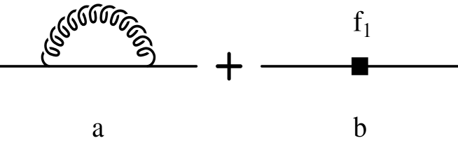
FIG. 4.:

\begin{picture}(10.0,15.0)\end{picture}

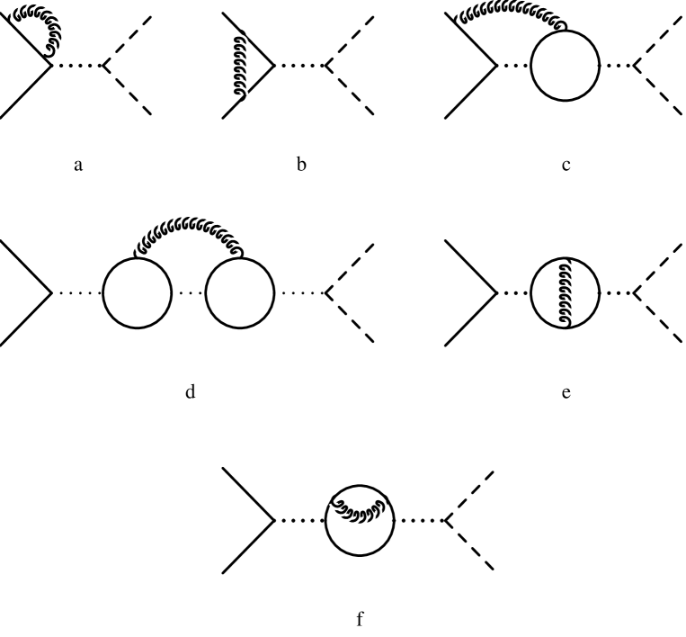
FIG. 5.:

\begin{picture}(10.0,15.0)\end{picture}

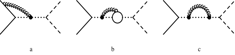
FIG. 6.:

\begin{picture}(10.0,15.0)\end{picture}

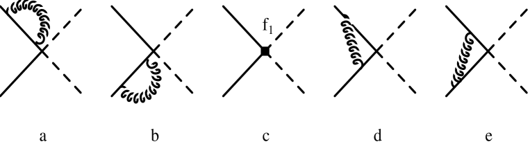
FIG. 7.:

\begin{picture}(10.0,15.0)\end{picture}

FIG. 8.:

REFERENCES

- [1] B. Adeva et al., CERN proposal CERN/SPSLC 95-1 (1995).
- [2] S. Deser, M.L. Goldberger, K. Baumann, and W. Thirring, Phys. Rev. 96, 774 (1954).
- [3] J.L. Uretsky and T.R. Palfrey, Jr., Phys. Rev. 121, 1798 (1961); S.M. Bilenky, Van Kheu Nguyen, L.L. Nemenov, and F.G. Tkebuchava, Sov. J. Nucl. Phys. 10, 469 (1969).
-
[4]
G. Colangelo, J. Gasser and H. Leutwyler,
Phys. Lett. B 488, 261 (2000)
[hep-ph/0007112]; Preprint hep-ph/0103088. - [5] M. Knecht, B. Moussallam, J. Stern, and N.H. Fuchs, Nucl. Phys. B 457, 513 (1995) [hep-ph/9507319]; ibid. B 471, 445 (1996) [hep-ph/9512404].
- [6] S. Weinberg, Physica A 96, 327 (1979).
- [7] J. Gasser and H. Leutwyler, Ann. Phys. (N.Y.) 158, 142 (1984).
- [8] J. Gasser and H. Leutwyler, Nucl. Phys. B 250, 465 (1985).
-
[9]
G. Colangelo, M. Knecht and J. Stern, Phys. Lett. B 336, 543 (1994)
[hep-ph/9406211];
G. Amoros, J. Bijnens and P. Talavera, Nucl. Phys. B 585 (2000) 293
[hep-ph/0003258];
G. Colangelo, J. Gasser and H. Leutwyler, Preprint hep-ph/0103063.
The literature on the subject may be traced form these references. - [10] A. Gall, J. Gasser, V.E. Lyubovitskij, and A. Rusetsky, Phys. Lett. B 462, 335 (1999) [hep-ph/9905309].
-
[11]
J. Gasser, V.E. Lyubovitskij and A. Rusetsky,
Newslett. 15, 185 (1999)
[hep-ph/9910524]; 15, 197 (1999) [hep-ph/9911260]. -
[12]
J. Gasser, V.E. Lyubovitskij and A. Rusetsky,
Phys. Lett. B 471, 244 (1999)
[hep-ph/9910438]. - [13] T.L. Trueman, Nucl. Phys. 26, 57 (1961).
-
[14]
U. Moor, G. Rasche, and W.S. Woolcock, Nucl. Phys. A 587, 747 (1995);
A. Gashi, G.C. Oades, G. Rasche, and W.S. Woolcock, Nucl. Phys. A 628, 101 (1998)
[nucl-th/9704017]. - [15] P. Minkowski, Preprint hep-ph/9808387.
- [16] G.V. Efimov, M.A. Ivanov, and V.E. Lyubovitskij, Sov. J. Nucl. Phys. 44, 296 (1986).
- [17] A.A. Bel’kov, V.N. Pervushin, and F.G. Tkebuchava, Sov. J. Nucl. Phys. 44, 300 (1986).
- [18] M.K. Volkov, Theor. Math. Phys. 71, 606 (1987).
- [19] Z. Silagadze, JETP Lett. 60, 689 (1994) [hep-ph/9411382]; E.A. Kuraev, Phys. Atom. Nucl. 61, 239 (1998); U. Jentschura, G. Soff, V. Ivanov, and S.G. Karshenboim, Phys. Lett. A 241, 351 (1998).
-
[20]
H. Jallouli and H. Sazdjian, Phys. Rev. D 58, 014011 (1998)
[hep-ph/9706450];
H. Sazdjian, Preprint hep-ph/9809425; Phys.Lett. B 490, 203 (2000) [hep-ph/0004226]. -
[21]
V.E. Lyubovitskij and A.G. Rusetsky, Phys. Lett. B 389, 181 (1996)
[hep-ph/9610217];
V.E. Lyubovitskij, E.Z. Lipartia, and A.G. Rusetsky,
JETP Lett. 66, 783 (1997)
[hep-ph/9801215]; M.A. Ivanov, V.E. Lyubovitskij, E.Z. Lipartia, and A.G. Rusetsky, Phys. Rev. D 58, 094024 (1998) [hep-ph/9805356]. - [22] P. Labelle and K. Buckley, Preprint hep-ph/9804201.
-
[23]
X. Kong and F. Ravndal, Phys. Rev. D 59, 014031 (1999);
Phys. Rev. D 61, 077506 (2000) [hep-ph/9905539]. - [24] B.R. Holstein, Phys. Rev. D 60, 114030 (1999) [nucl-th/9901041].
- [25] D. Eiras and J. Soto, Newslett. 15, 181 (1999);
- [26] D. Eiras and J. Soto, Phys. Rev. D 61, 114027 (2000) [hep-ph/9905543];
- [27] D. Eiras and J. Soto, Phys. Lett. B 491, 101 (2000) [hep-ph/0005066].
- [28] W.E. Caswell and G.P. Lepage, Phys. Lett. B 167, 437 (1986).
- [29] H. Feshbach, Ann. Phys. 5, 357 (1958); ibid 19, 287 (1962).
-
[30]
V. Antonelli, A. Gall, J. Gasser, and A. Rusetsky,
Ann. Phys. 286, 108 (2000)
[hep-ph/0003118]. - [31] V.E. Lyubovitskij and A.G. Rusetsky, Phys. Lett. B 494, 9 (2000) [hep-ph/0009206].
- [32] J. Schwinger, J. Math. Phys. 5, 1606 (1964).
- [33] D.R. Yennie, S.C. Frautschi, and H. Suura, Ann. Phys. 13, 379 (1961).
- [34] M. Knecht and R. Urech, Nucl. Phys. B 519, 329 (1998) [hep-ph/9709348].
- [35] F.S. Roig and A.R. Swift, Nucl. Phys. B 104, 533 (1976).
- [36] R. Urech, Nucl. Phys. B 433, 234 (1995) [hep-ph/9405341].
- [37] R. Baur and R. Urech, Nucl. Phys. B 499, 319 (1997) [hep-ph/9612328].
- [38] B. Moussallam, Nucl. Phys. B 504, 381 (1997) [hep-ph/9701400].
- [39] J. Bijnens and J. Prades, Nucl. Phys. B 490, 239 (1997) [hep-ph/9610360].
- [40] J. Gasser and H. Leutwyler, Phys. Rep. 87, 77 (1982).
- [41] H.W. Hammer and J.N. Ng, Eur. Phys. J. A 6, 115 (1999) [hep-ph/9902284].
- [42] J. Bijnens, G. Colangelo, G. Ecker, J. Gasser, and M.E. Sainio, Nucl. Phys. B 508, 263 (1997) [hep-ph/9707291].
- [43] M. Beneke and V.A. Smirnov, Nucl. Phys. B 522, 321 (1998) [hep-ph/9711391].
- [44] A.V. Manohar, Phys. Rev. D 56, 230 (1997) [hep-ph/9701294]; A. Pineda and J. Soto, Nucl. Phys. Proc. Suppl. 64, 428 (1998) [hep-ph/9707481]; Phys. Lett. B 420, 391 (1998) [hep-ph/9711292]; Phys. Rev. D 58, 114011 (1998) [hep-ph/9802365]; Phys. Rev. D 59, 016005 (1999) [hep-ph/9805424].
- [45] J. Soto, private communication.
-
[46]
D.J. Broadhurst, J. Fleischer, and O.V. Tarasov,
Z. Phys. C 60, 287 (1993)
[hep-ph/9304303].