Possibility of T-violating P-conserving magnetism and its contribution to the T-odd P-even neutron-nucleus forward elastic scattering amplitude.

Abstract

T-violating P-even magnetism is considered. The magnetism arises from the T-violating P-conserving vertex of a spin 1/2 particle interaction with the electromagnetic field. The vertex varnishes for a particle on the mass shell. Considering the particle interaction with a point electric charge we have obtained the T-violating P-even spin dependent potential which is inversely proportional to the cubed distance from the charge. The matrix element of this potential is zero for particle states on the mass shell, nevertheless, the potential contributes to the T-odd P-even neutron forward elastic scattering amplitude by a deformed nucleus with spin $S>1/2$. The contribution arises if we take into account incident neutron plane wave distortion by the strong neutron interaction with the nucleus.

1 Introduction

In connection with the direct observation of time-reversal symmetry violation in the system of $K^{0}-\bar{K}^{0}$ mesons cplear it would be interesting to detect T-violation in other nuclear or atomic systems. However, the Standard Model predicts very small T-violating effects in nuclear and atomic physics, so we are forced to search for new interactions. It is necessary to distinguish a P- T- odd interaction from a P-even T-odd one. While there are rather rigid restrictions on the strength constants of the first type interactions, obtained from dipole moment measurements of atoms and particles, restrictions on the constants of P-even T-odd interactions are not so strong. As is known the null test for the latter kind of interaction is the observation of a $\sim(\boldsymbol{\sigma}\times\vec{k}\cdot\vec{S})(\vec{k}\cdot\vec{S})$ five fold correlation term in the forward elastic scattering amplitude of a spin $1/2$ particle by a particle with a spin $S\geq 1$ bar1 ; conzet ; beyer ; cher , where $\vec{k}$ is the incident particle momentum, $\boldsymbol{\sigma}$ is the Pauli matrix of an incident particle and $\vec{S}$ is the nucleus spin operator. The relevant experiments have been carried out exp ; huf0 for a ${}^{165}\mbox{Ho}$ target and now are planed to be performed on a super-conducting synchrotron COSY COSY with deuteron. Usually the P-conserving breakdown of the time reversal symmetry is considered on the basis of the $\rho$ and $A_{1}$ meson Lagrangian sim . In this paper we consider another phenomenological possibility, namely, T-violating P-conserving magnetism and its contribution to the aforementioned five fold correlation.

2 Long-range T-non-invariant P-even electromagnetic interaction.

The magnetism can be introduced by the T-violating P-conserving vertex function of a spin 1/2 particle interaction with the electromagnetic field t1 ; haff :

$$\Gamma^{\eta}_{T}=\mu_{T}\frac{\mbox{i}}{2\,m^{3}}(Pq)\sigma^{\eta\nu}q_{\nu}~{},$$ (1)

where $P=k^{\prime}+k$, $q=k^{\prime}-k$ (Fig. 1), $m$ is the particle mass and $\sigma^{\eta\nu}=\frac{\gamma^{\eta}\gamma^{\nu}-\gamma^{\nu}\gamma^{\eta}}{2}$. Let us consider T-odd scattering of a particle by a point electric charge $Ze$.

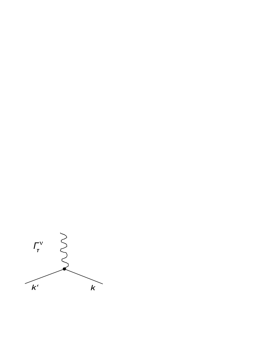
Figure 1: T-odd P-even vertex of the particle interaction with the electromagnetic field.

After the application of ordinary diagram techniques ber we obtain the appropriate matrix element corresponding to the diagram in Fig. 1:

$${\mathcal{M}}=-\mu_{T}\frac{\mbox{i}e}{2\,m^{3}}(Pq)\bar{u}(k^{\prime})\sigma^{0\nu}q_{\nu}u(k){\mathcal{A}}^{(e)}_{0}~{},$$ (2)

where ${\mathcal{A}}^{(e)}_{0}(q)=\frac{4\,\pi Ze}{\vec{q}^{2}}$ is the Fourier transform of the Coulomb potential of the electric charge and $u(k)$ is the particle bispinor. Setting $q=(0,\vec{q})$ and substituting

$$u(k)=\left(\begin{array}[]{c}\sqrt{\varepsilon+m}\;\phi\\ (\varepsilon+m)^{-1/2}\;(\boldsymbol{\sigma}\vec{k})\;\phi\end{array}\right)~{}$$

($\phi$ is the spin wave function of a particle and $\varepsilon$ is the particle energy including its rest mass) into (2) we find the T-odd P-even scattering amplitude of a particle by a point electric charge for small transferred momentum $\vec{q}$:

$${\mathfrak{f}}(\vec{q})=\frac{\mathcal{M}}{4\pi}=-\mu_{T}\frac{2Ze^{2}}{m^{3}}\frac{(\vec{k}\vec{q})(\boldsymbol{\sigma}\times\vec{k}\cdot\vec{q})}{\vec{q}^{2}}.$$ (3)

While evaluating the scattering amplitude we consider a particle to be on the mass shell $(\vec{k}^{2}=(\vec{k}+\vec{q})^{2}=\varepsilon^{2}-m^{2})$ everywhere except for the term $(\vec{k}\vec{q})$. If the particle is completely on the mass shell $(\vec{k}\vec{q})=0$ and the amplitude (3) vanishes. The dependence of the amplitude on the transferred momentum $\vec{q}$ looks like that for the magnetic dipoles scattering amplitude. So, it turns out that the interaction is long-range. In haff the conclusion (repeated in the monograph of blin ) had been drawn of the non-existence of a long-range T-odd P-even potential (i.e. it is decreasing as $1/r^{3}$ or weaker with distance Dau ). However, we’ll see that this conclusion does not concern of-mass-shell potentials.

We can consider the particle scattering in the framework of the Schroedinger equation with relativistic mass ber ; for :

$$(\nabla^{2}+\vec{k}^{2})\Psi({\vec{r}})=2\varepsilon V(\vec{r})\Psi(\vec{r}),$$ (4)

which allows us below to take into account incident particle wave distortion by the strong nucleus interaction. In the first Born approximation the amplitude (3) can be obtained from the T-odd energy dependent interaction:

$${V}_{T}(\boldsymbol{r})=-\mu_{T}\ \frac{3Ze^{2}}{2\varepsilon m^{3}}\bigl{(}(\hat{\vec{p}}\vec{r})\frac{1}{r^{5}}(\vec{r}\cdot\boldsymbol{\sigma}\times\hat{\vec{p}})$$

$$+(\boldsymbol{\sigma}\times\hat{\vec{p}}\cdot\vec{r})\frac{1}{r^{5}}(\vec{r}\hat{\vec{p}})\bigr{)}~{}.$$ (5)

It can be represented by:

$${V}_{T}(\vec{r})=\mu_{T}\frac{e}{2\varepsilon m^{3}}\bigl{(}\hat{\vec{p}}\cdot\{\vec{\nabla}\otimes\vec{E}(\vec{r})\}$$

$$\cdot(\boldsymbol{\sigma}\times\hat{\vec{p}})+(\boldsymbol{\sigma}\times\hat{\vec{p}})\cdot\{\vec{\nabla}\otimes\vec{E}(\vec{r})\}\cdot\hat{\vec{p}}\bigr{)},$$ (6)

where $\vec{E}(\vec{r})=-\vec{\nabla}\Phi(\vec{r})=Ze{\displaystyle\frac{\vec{r}}{r^{3}}}$ is the strength of the electric field created by a charge at the point $\vec{r}$, the gradient acts on the $\vec{E}(\vec{r})$ only, $\hat{\vec{p}}$ is the particle momentum operator and $\otimes$ denotes a direct vector product. When considering a particle moving along classical trajectory, we should replace the momentum operator by its classical value.

Figure 2: Scematic picture of classical particle trajectories (in the first order in interaction) calculated with the classical Hamiltonian obtained from the of-the-mass-shell interaction through replacing particle momentum operator by its classical value.

In the first order in interaction the trajectories of a classical particle deflect from a straight line only in the vicinity of a scatter (Fig. 2). In the presence of some ordinary on-mass-shell interaction, for instance strong one, the of-mass-shell T-odd interaction decreases or increases the stream of particles in the area of strong interaction and, thereby, gives a T-odd contribution to the scattering amplitude.

So, we can see that a moving particle can interact with a non-uniform electric field by means of the time reversal violating parity conserving interaction.

3 T-odd scattering of a neutron by a deformed nucleus with spin $S\geq 1$

Let us consider T-odd neutron scattering by a deformed nucleus. Let us assume that interaction of a neutron with a nucleus is the sum of the T-odd interaction, discussed above, and the strong one. For evaluating the neutron-nucleus elastic scattering amplitude we’ll use the Schroedinger equation (4). The scattering amplitude at zero angle in the third Born approximation is written as

$$F(\vec{k},\vec{k})=-\frac{\varepsilon}{2\pi}\Biggl{\{}U(\vec{k},\vec{k})~{}~{}~{}~{}~{}~{}~{}~{}~{}~{}~{}~{}~{}~{}~{}~{}~{}~{}~{}~{}~{}~{}~{}~{}~{}~{}~{}~{}~{}~{}$$

$$+2\varepsilon\int\frac{U(\vec{k},\vec{k}^{\prime})U(\vec{k}^{\prime},\vec{k})}{k^{2}-k^{\prime 2}+i0}\frac{d^{3}\vec{k}^{\prime}}{(2\pi)^{3}}~{}~{}~{}~{}~{}$$

$$+(2\varepsilon)^{2}\int\frac{U(\vec{k},\vec{k}^{\prime})U(\vec{k}^{\prime},\vec{k}^{\prime\prime})U(\vec{k}^{\prime\prime},\vec{k})}{(k^{2}-k^{\prime 2}+i0)(k^{2}-k^{\prime\prime 2}+i0)}\frac{d^{3}\vec{k}^{\prime}}{(2\pi)^{3}}\frac{d^{3}\vec{k}^{\prime\prime}}{(2\pi)^{3}}$$

$$+\cdots\Biggr{\}},$$ (7)

where $U(\vec{k}^{\prime},\vec{k})=\int\mbox{e}^{-i\vec{k}^{\prime}\vec{r}}V(\vec{r})\mbox{e}^{i\vec{k}\vec{r}}d^{3}\vec{r}$ represents the Fourier transform of the neutron-nucleus potential. $U(\vec{k}^{\prime},\vec{k})$ is the sum of the strong interaction part (for simplicity we consider it is not to be depending on the spin) and T-odd one:

$$U(\vec{k}^{\prime},\vec{k})=u_{s}(\vec{k}^{\prime}-\vec{k})+\bigl{(}\boldsymbol{\sigma}\cdot(\vec{k}^{\prime}+\vec{k})\times(\vec{k}^{\prime}$$

$$-\vec{k})\bigr{)}\bigl{(}(\vec{k}^{\prime}+\vec{k})\cdot(\vec{k}^{\prime}-\vec{k})\bigr{)}u_{T}(\vec{k}^{\prime}-\vec{k}).$$ (8)

For the nucleus with the centre of symmetry $u_{s}(\vec{k})=u_{s}(-\vec{k})$ and $u_{T}(\vec{k})=u_{T}(-\vec{k})$. Substituting (8) in (7) we find that the first and second Born terms give zero contributions. As a result, we have

$$F_{T}(\vec{k},\vec{k})=-\frac{2\varepsilon^{3}}{\pi}\int\Biggl{\{}2\bigl{(}\boldsymbol{\sigma}\times(\vec{k}^{\prime}+\vec{k})\cdot(\vec{k}-\vec{k}^{\prime})\bigr{)}\frac{1}{k^{2}-k^{\prime\prime 2}}$$

$$\times u_{T}(\vec{k}-\vec{k}^{\prime})u_{s}(\vec{k}^{\prime}\vec{-}k^{\prime\prime})u_{s}(\vec{k}^{\prime\prime}-\vec{k})+\bigl{(}\boldsymbol{\sigma}\times(\vec{k}^{\prime}+\vec{k}^{\prime\prime})$$

$$\cdot(\vec{k}^{\prime}-\vec{k}^{\prime\prime})\bigr{)}\frac{((\vec{k}^{\prime\prime}+\vec{k}^{\prime})(\vec{k}^{\prime}-\vec{k}^{\prime\prime}))}{(k^{2}-k^{\prime 2})(k^{2}-k^{\prime\prime 2})}u_{s}(\vec{k}-\vec{k}^{\prime})$$

$$\times u_{T}(\vec{k}^{\prime}-\vec{k}^{\prime\prime})u_{s}(\vec{k}^{\prime\prime}-\vec{k})\Biggr{\}}\frac{d^{3}\vec{k}^{\prime}}{(2\pi)^{3}}\frac{d^{3}\vec{k}^{\prime\prime}}{(2\pi)^{3}}.~{}~{}~{}~{}~{}$$ (9)

In the first item of (9) we change variables $\vec{k}^{\prime}=\vec{k}+\vec{q},~{}\vec{k}^{\prime\prime}=\vec{k}+\vec{Q}$, and in the second item $\vec{k}^{\prime}=\vec{k}+\vec{Q}-\vec{q},~{}~{}\vec{k}^{\prime\prime}=\vec{k}+\vec{Q}$ and come to

$$F_{T}(\vec{k},\vec{k})=-\frac{2\varepsilon^{3}}{\pi}\int\Biggl{\{}-2(\boldsymbol{\sigma}\times\vec{k}\cdot\vec{q})\biggl{(}\frac{1}{k^{2}-(\vec{k}+\vec{Q})^{2}}$$

$$+\frac{1}{k^{2}-(\vec{k}+\vec{Q}-\vec{q})^{2}}\biggr{)}+2(\boldsymbol{\sigma}\times\vec{Q}\cdot\vec{q})\biggl{(}\frac{1}{k^{2}-(\vec{k}+\vec{Q})^{2}}$$

$$-\frac{1}{k^{2}-(\vec{k}+\vec{Q}-\vec{q})^{2}}\biggr{)}\Biggr{\}}u_{T}(\vec{q})u_{s}(\vec{q}-\vec{Q})u_{s}(\vec{Q})$$

$$\times\frac{d^{3}\vec{q}}{(2\pi)^{3}}\frac{d^{3}\vec{Q}}{(2\pi)^{3}}=-\frac{8\varepsilon^{3}}{\pi}\int(\boldsymbol{\sigma}\times\vec{Q}\cdot\vec{q})\frac{1}{k^{2}-(\vec{k}+\vec{Q})^{2}}$$

$$\times u_{T}(\vec{q})u_{s}(\vec{q}-\vec{Q})u_{s}(\vec{Q})\frac{d^{3}\vec{q}}{(2\pi)^{3}}\frac{d^{3}\vec{Q}}{(2\pi)^{3}}.~{}~{}~{}~{}~{}$$ (10)

Deriving the last equality we have changed the variables $\vec{Q}=\vec{Q}^{\prime}-\vec{q}^{\prime}$, $\vec{q}=-\vec{q}^{\prime}$ in terms containing the factor $\frac{1}{k^{2}-(\vec{k}+\vec{Q}-\vec{q})^{2}}$. Using the formula (6) we express $u_{T}(\vec{k})$ through the Fourier transform of the charge distribution function inside the nucleus $\rho(\vec{k})$ (nucleus charge form factor):

$$u_{T}(\vec{k})=\mu_{T}\frac{\pi Ze^{2}}{\varepsilon m^{3}}\frac{\rho(\vec{k})}{k^{2}}.$$ (11)

In the rough approximation, being suitable however for our purposes, the strong interaction term can also be expressed through the Fourier transform of the nucleon distribution function in the nucleus and the nucleon-nucleon scattering amplitude at zero angle $f(0)$ :

$$u_{s}(\vec{k})=-\frac{2\pi Af(0)}{\varepsilon}\rho(\vec{k}),$$ (12)

where $A$ is the atomic number of the nucleus. Thus, we assume, that the charge distribution coincides with the matter density. From (10) we come to

$$F_{T}(\vec{k},\vec{k})=-\mu_{T}\frac{8Ze^{2}}{m^{3}}(2\pi)^{2}A^{2}f^{2}(0)$$

$$\times\int\frac{(\boldsymbol{\sigma}\times\vec{Q}\cdot\vec{q})}{k^{2}-(\vec{k}+\vec{Q})^{2}+i0}\frac{\rho(\vec{q})\rho(\vec{q}-\vec{Q})\rho(\vec{Q})}{q^{2}}$$

$$\times\frac{d^{3}\boldsymbol{q}}{(2\pi)^{3}}\frac{d^{3}\vec{Q}}{(2\pi)^{3}}$$ (13)

At high energies a simplification can be achieved by using the propagator in the eikonal approximation:

$$\frac{1}{k^{2}-(\vec{k}+\vec{Q})^{2}+i0}\approx\frac{1}{-2\vec{k}\vec{Q}+i0}=-P\frac{1}{2\vec{k}\vec{Q}}-i\pi\delta(2\vec{k}\vec{Q}).$$ (14)

The contribution of the first term of (14) vanishes as can be checked by changing of the variables $\vec{Q}=-\vec{Q}^{\prime}$, $\vec{q}=-\vec{q}^{\prime}$ in the expression (13). The deformed nucleus form factor can be taken in the form:

$$\rho(\vec{q})=\mbox{e}^{-\beta q^{2}+\beta^{\prime}(\boldsymbol{a}\vec{q})^{2}}.$$ (15)

The unit vector $\boldsymbol{a}$ is parallel to the axis of symmetry of the nucleus ($z$-axis) and describes the orientation of the nucleus. The expression (15) corresponds to the charge and matter distribution function:

$$\wp(\vec{r})=\frac{1}{(2\pi)^{3}}\int\mbox{e}^{i\vec{q}\vec{r}}\rho(\vec{q})d^{3}\vec{q}~{}~{}~{}~{}~{}~{}~{}~{}~{}~{}~{}~{}$$

$$=\frac{1}{8\pi^{3/2}\beta\sqrt{\beta-\beta^{\prime}}}\exp{\left(-\frac{r^{2}}{4\beta}-\frac{\beta^{\prime}z^{2}}{4\beta(\beta-\beta^{\prime})}\right)}.$$ (16)

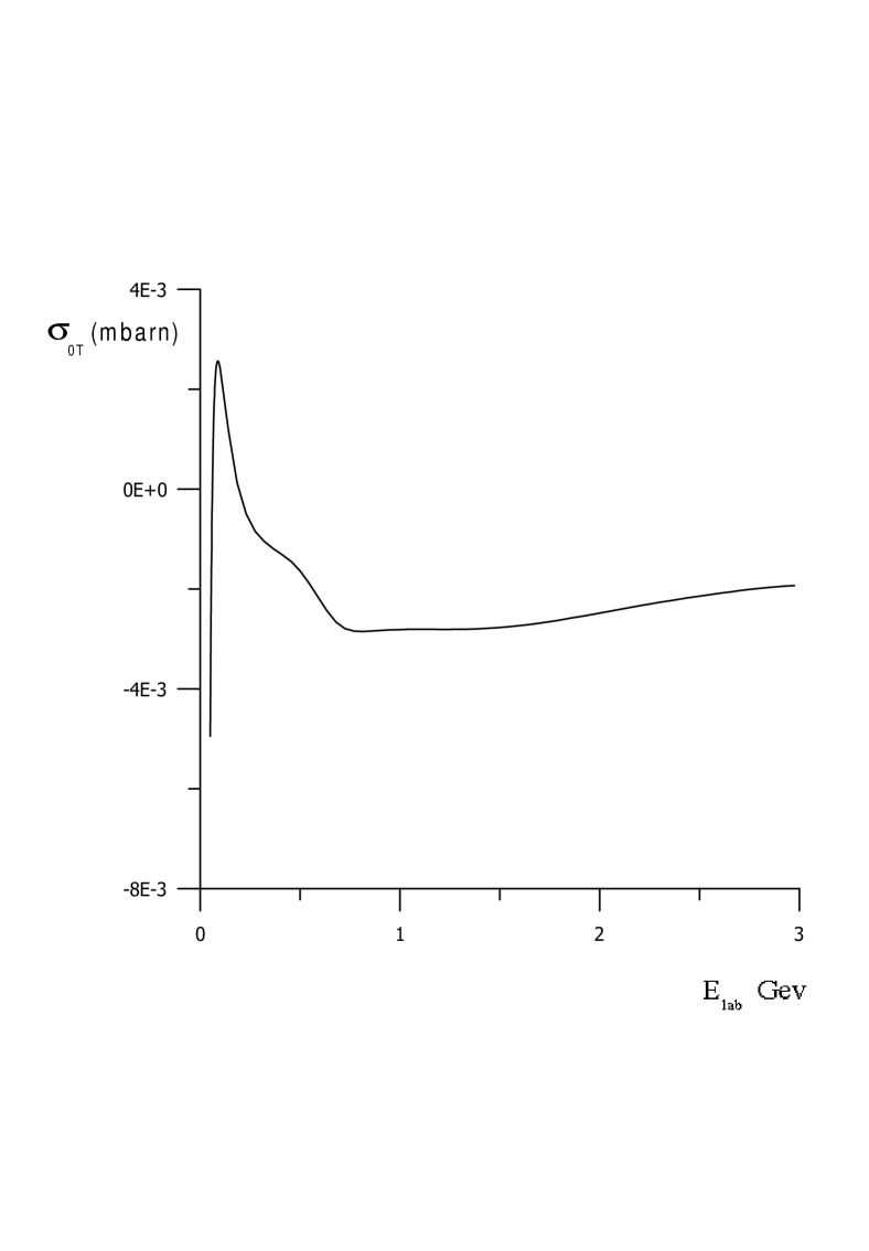
Figure 3: T-violating P-even cross section $\sigma_{\mbox{\tiny T}}=\sigma_{\mbox{\tiny 0T}}(\boldsymbol{\sigma}\cdot\vec{S}\times{\vec{k}\over k})(\vec{S}\cdot{\vec{k}\over k})$ for ${}^{165}\mbox{Ho}$ target at T-violating moment $\mu_{T}=1$.

$\beta^{\prime}$ characterises the degree of deformation of the nucleus and is connected with the quadruple moment

$${\mathcal{Q}}=Z\int(3z^{2}-r^{2})\wp(\vec{r})d^{3}\vec{r}=-4\,Z\beta^{\prime}.$$ (17)

For a small nucleus deformation the nucleus root-mean-square radius is expressed through $\beta$:

$$R^{2}=\int r^{2}\wp(r)d^{3}r\approx 6\beta.$$ (18)

The calculation of the integral In the first order in $\beta^{\prime}$ gives the following expression:

$$\int\vec{Q}\times\vec{q}\frac{\delta(\vec{k}\vec{Q})}{q^{2}}\exp\bigl{(}-\beta q^{2}+\beta^{\prime}(\boldsymbol{a}\vec{q})^{2}-\beta(\vec{q}-\vec{Q})^{2}$$

$$+\beta^{\prime}(\boldsymbol{a}\cdot(\vec{q}-\vec{Q}))^{2}-\beta\vec{Q}^{2}+\beta^{\prime}(\boldsymbol{a}\vec{Q})^{2}\bigr{)}d^{3}\vec{Q}d^{3}\vec{q}$$

$$\approx(\boldsymbol{a}\times\vec{k})(\boldsymbol{a}\cdot\vec{k})\frac{\pi^{5/2}}{2k^{3}}\frac{\beta^{\prime}}{\beta^{2}}$$

$$\times\int_{\beta}^{\infty}\frac{\beta-x}{(2x+\beta)^{2}(\beta+x)^{3/2}}dx.$$ (19)

With the help of (19) we obtain the final formula:

$$F_{T}(\vec{k},\vec{k})=i(\boldsymbol{\sigma}\cdot\boldsymbol{a}\times\vec{k})(\boldsymbol{a}\cdot\vec{k})\mu_{T}$$

$$\times\frac{Ze^{2}A^{2}f^{2}(0)}{8\sqrt{\pi}m^{3}k^{3}}\frac{\beta^{\prime}}{\beta^{7/2}}\int_{1}^{\infty}\frac{(1-x)dx}{(2x+1)^{2}(1+x)^{3/2}}.$$ (20)

The unit vector $\boldsymbol{a}$ is expressed thorough the only available nucleus spin operator vector : $\boldsymbol{a}={\vec{S}\over{\sqrt{S(S+1)}}}$. Setting T-violating moment (expressed in $e/2m$ units) $\mu_{T}=1$ we find that T-odd cross section is about of $10^{-3}$ mbarn (Fig.3) for a ${}^{165}\mbox{Ho}$ ($S=7/2$) target.

It is possible to obtain the formula for the limiting case of low energies, however, the approximation (12) used for the strong interaction becomes very rough. At low energies the propagator can be approximated by:

$$\frac{1}{k^{2}-(\vec{k}+\vec{Q})^{2}+i0}\approx-\frac{1}{Q^{2}}+\frac{2\vec{k}\vec{Q}}{Q^{4}}-\frac{4(\vec{k}\vec{Q})^{2}}{Q^{6}}.$$ (21)

The final formula at low energies looks like:

$$F_{T}(\vec{k},\vec{k})=(\boldsymbol{\sigma}\cdot\boldsymbol{a}\times\vec{k})(\boldsymbol{a}\cdot\vec{k})\mu_{T}$$

$$\times\frac{8Ze^{2}A^{2}f^{2}(0)}{15\pi m^{3}}\frac{\beta^{\prime}}{\beta^{2}}\int_{1}^{\infty}\frac{(1-x)dx}{(x+1)^{3}\sqrt{2x+1}}$$ (22)

A magnitude of the amplitude is proportional to the squared neutron wave number $k^{2}$ at low energies, whereas at high energies it decreases in inverse proportion to the wave number. At $kR\sim 1$ both formulas give the same but overestimated order of the amplitude magnitude. So, we restrict ourselves $\varepsilon-m=\mbox{E}_{\mbox{\tiny lab}}>50~{}~{}Mev$ (Fig.3), where $kR>7$ and the eikonal approximation should be valid.

4 Estimates for T-odd magnetism for the other systems.

It is of interest to study the consequences of T-violating P-conserving magnetism for other systems.

a) Electric dipole moment (EDM) of a neutron. The existing rigid experimental limit on the neutron EDM ($8\times 10^{-26}e~{}cm$) allows one to obtain constraints on the T-odd P-even interactions. Actually we have $P-odd~{}~{}T-odd=(P-even~{}~{}T-odd)\times(P-odd~{}~{}T-even)$. So, P-conserving beakdown of the time reversal symmetry contributes to the neutron EDM through interference with P-odd weak interaction.

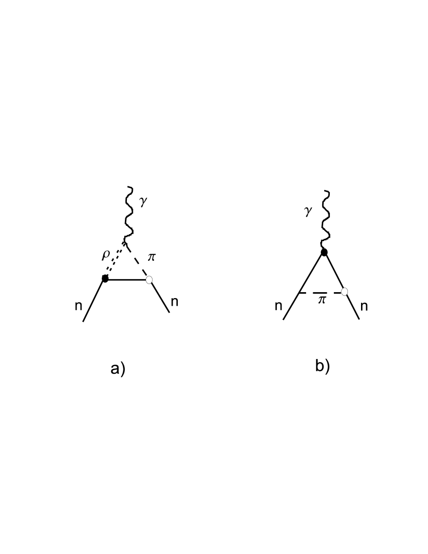
Figure 4: Diagrams contributing to the neutron EDM. Black circles denote T-odd P-even vertexes, white circles denote P-odd T-even vertexes.

The restriction $\bar{g}_{\rho}<10^{-3}$ on the relative magnitude of the T-odd P-even nucleon-$\rho$-meson coupling has been obtained haxt by calculating the Feynman graph in Fig. 4a. The source of T-violation was the $\rho$-meson-nucleon vertex and the source of P-violation was the $\pi$-meson-neutron interaction.

We can consider the diagram in Fig.4b, corresponding to the T-odd magnetism contribution to the neutron EDM. Both diagrams contain strong, electromagnetic and weak interaction vertices. Hence they should give approximately the same restriction on the relative strength of the T-violation, but, in the first case, T-violation occurs in strong interaction, and in the second case it occurs in the electromagnetic one. However, due to the of-mass-shell character of the electromagnetic vertex an additional suppression factor $\frac{(Pq)}{m^{2}}\sim\left(\frac{m_{\pi}}{m}\right)^{2}\approx 2\times 10^{-2}$ arises haff . Thus the constraint on $\mu_{T}$ is expected to be $\mu_{T}\sim 10^{-1}$.

b) positronium-like system decays. Let us now consider the positronium system. The density of electrons (positrons) in positronium state with total spin $J=1$ can be presented in the form cher

$$\rho(\vec{r})=A_{0}(r)+A_{1}\vec{J}\left(\boldsymbol{\sigma}_{-}+\boldsymbol{\sigma}_{+}\right)+A_{2}(\vec{J}\vec{r})(\boldsymbol{\sigma}_{-}+\boldsymbol{\sigma}_{+})\cdot\vec{r}$$

$$+\dots+T_{0}(\boldsymbol{\sigma}_{-}\times\boldsymbol{\sigma}_{+}\cdot\vec{J})+T_{1}((\boldsymbol{\sigma}_{-}\vec{r})(\boldsymbol{\sigma}_{+}\times\vec{J}\cdot\vec{r})$$

$$-(\boldsymbol{\sigma}_{+}\vec{r})(\boldsymbol{\sigma}_{-}\times\vec{J}\cdot\vec{r}))+T_{2}((\vec{J}\vec{r})((\boldsymbol{\sigma}_{-}-\boldsymbol{\sigma}_{+})\times\vec{J}\cdot\vec{r})$$

$$+((\boldsymbol{\sigma}_{-}-\boldsymbol{\sigma}_{+})\times\vec{J}\cdot\vec{r})(\vec{J}\vec{r})),~{}~{}~{}~{}~{}~{}$$ (23)

where $\vec{r}$ is the electron radius vector (the positron radius-vector is $-\vec{r}$ ), $A_{n},T_{n}$ are the functions of $r$, $\boldsymbol{\sigma}_{-}$, $\boldsymbol{\sigma}_{+}$ are the Pauli matrices of electron and positron, respectively. The density is simultaneously the spin density matrix of a positron and an electron. The positronium total spin operator $\vec{J}$ is a parameter describing the positronium orientation. To find the density for the concrete positronium orientation we must take the matrix element from (23) over a positronium spin state i.e. replace $\vec{J}$ and $\vec{J}\otimes\vec{J}$ through the positronium polarization $<\vec{J}>$ and quadropolarization $<\vec{J}\otimes\vec{J}>$ respectively. The result of C-, P-, T- transformations on the density can be described by the operations

$$C:\boldsymbol{\sigma}_{+}\rightarrow{\boldsymbol{\sigma}}_{-},~{}~{}\boldsymbol{\sigma}_{-}\rightarrow\boldsymbol{\sigma}_{+},~{}~{}\vec{r}\rightarrow-\vec{r}~{},$$

$$T:\vec{J}\rightarrow-\vec{J},~{}~{}\boldsymbol{\sigma}_{+}\rightarrow-{\boldsymbol{\sigma}}_{+},~{}~{}\boldsymbol{\sigma}_{-}\rightarrow-\boldsymbol{\sigma}_{-}~{},$$

$$P:\vec{r}\rightarrow-\vec{r}.~{}~{}~{}~{}~{}~{}~{}~{}~{}~{}~{}~{}~{}~{}~{}~{}~{}~{}~{}~{}~{}~{}~{}~{}~{}~{}~{}~{}~{}~{}~{}~{}~{}~{}~{}~{}~{}$$ (24)

We can see that the terms proportional to $T_{0},T_{1},T_{2}$ are T-odd, C-odd, P-even terms. But, it is not possible to construct T-odd P-even terms for the states with $J=0$. From this fact we may conclude that decays of positronium like systems with $1$ spin should be used to search indirect T- C-violation.

The terms $T_{0},\dots$ can originate from mixing of the states with the same spatial parity but opposite charge parity due to the P-even T-odd C-odd interaction

$${V}_{T}(\boldsymbol{r})=-\mu_{T}\ \frac{3e^{2}}{2\varepsilon m^{3}}\bigl{(}(\hat{\vec{p}}\vec{r})\frac{1}{r^{5}}(\vec{r}\cdot(\boldsymbol{\sigma}_{-}-\boldsymbol{\sigma}_{+})\times\hat{\vec{p}})$$

$$+((\boldsymbol{\sigma}_{-}-\boldsymbol{\sigma}_{+})\times\hat{\vec{p}}\cdot\vec{r})\frac{1}{r^{5}}(\vec{r}\hat{\vec{p}})\bigr{)}~{},$$ (25)

where $\mu_{T}$ is the T-violating electron moment (the positron has the same) and $m$ is the electron mass. However for the orto-positronium state ${}^{3}S_{1}~{}(J^{PC}=1^{--})$ there is no the state with $J^{PC}=1^{-+}$ which can be mixed to it. The charge parity of positronium is given by $C=(-1)^{l+s}$ and the spatial parity is given by $P=(-1)^{l+1}$. So T- C- violation can occurs only in the direct decay not under consideration here. For the state ${}^{1}P_{1}~{}(J^{PC}=1^{+-})$ there exists a state ${}^{3}P_{1}~{}(J^{PC}=1^{++})$ which can mixed to it. The impurity can be estimated as $\eta_{T}\sim\frac{V_{T}}{\Delta E}$, where $V_{T}$ is the typical value of a T-odd interaction and $\Delta E$ is the splitting between these levels. The splitting $\Delta E$ can be produced by tensor and spin-orbital interactions ber

$$V_{s}=\frac{3\alpha}{4m^{2}}\frac{1}{r^{3}}\biggl{(}\bigl{(}\vec{r}\times\vec{p}\cdot(\boldsymbol{\sigma}_{-}+\boldsymbol{\sigma}_{+})\bigr{)}$$

$$+\frac{(\boldsymbol{\sigma}_{-}\vec{r})(\boldsymbol{\sigma}_{+}\vec{r})}{r^{2}}-\frac{1}{3}(\boldsymbol{\sigma}_{-}\boldsymbol{\sigma}_{+})\biggr{)},$$ (26)

where $\alpha=e^{2}$ is the fine structure constant. Typical values of an electron momentum and co-ordinate in positronium are $p\sim m\alpha,~{}~{}r\sim\frac{1}{m\alpha}$ ber . Thus, we can estimate $V_{T}$ to be

$$V_{T}\sim\mu_{T}\frac{\alpha}{m^{4}}\frac{p^{2}}{r^{3}}\sim\mu_{T}m\alpha^{6}$$ (27)

and

$$\Delta E\sim V_{s}\sim\frac{\alpha}{m^{2}}\frac{p}{r^{2}}\sim m\alpha^{4}.$$ (28)

As a result, for the C- and T- odd impurity of the ${}^{3}P_{1}$ state to the ${}^{1}P_{1}$ state we have

$$\eta_{T}\sim\frac{V_{T}}{\Delta E}\sim\mu_{T}\alpha^{2}.$$ (29)

For the branching ratio we get

$$\frac{\mathcal{R}(^{1}P_{1}\rightarrow^{3}S_{1}+\gamma)}{\mathcal{R}(^{1}P_{1}\rightarrow^{3}S_{1}+2\gamma)}\sim\frac{\eta_{T}}{\alpha}\sim\mu_{T}\alpha.$$ (30)

We take into account here that the probability of the decay into ${}^{3}S_{1}+2\gamma$ is reduced by an additional factor $\alpha$ compared to the decay to ${}^{3}S_{1}+\gamma$ ber . The measurement of the branching ratio (30) with the accuracy $10^{-2}$ gives constraint for electron’s $\mu_{T}\sim 1$, but it is far beyond the experimental possibilities of positronium physics by now.

Let us consider a charmonium $c\bar{c}$ system, which is similar to positronium. One gluon exchange produces the Coulomb-like potential with a running constant approximately equal to $\alpha_{s}=0.4$ led (applicable also for the tensor interaction). Charmonium energy levels can be described by this potential and a confinement potential of oscillator type. The later is essential for large excitations and it will not be taken into account in our estimations. Repeating our estimations for the present case we find:

$$V_{T}\sim\mu_{T}\frac{\alpha}{m_{c}^{4}}\frac{p^{2}}{r^{3}}\sim\mu_{T}m_{c}\alpha\,\alpha_{s}^{5},$$

$$\Delta E\sim\frac{\alpha_{s}}{m_{c}^{2}}\frac{p}{r^{2}}\sim m_{c}\alpha_{s}^{4},$$

$$\eta_{T}\sim\frac{V_{T}}{\Delta E}\sim\mu_{T}\alpha\,\alpha_{s},$$ (31)

where $m_{c}$ is the mass of a charmed quark. For the branching ratio of a $c\bar{c}$ system we find

$$\frac{\mathcal{R}(^{1}P_{1}\rightarrow J/\psi+\gamma)}{\mathcal{R}(^{1}P_{1}\rightarrow J/\psi+2\gamma)}\sim\frac{\eta_{T}}{\alpha}\sim\mu_{T}\alpha_{s}.$$ (32)

The ${}^{3}P_{1}$ state of charmonium has experimentally been identified and is called $\chi_{c1}(1P)(3510)$ part2 . The ${}^{1}P_{1}$ state has not been clearly identified by now. A possible candidate would be $h_{c}(1P)(3526)$, but this needs confirmation part2 .

c) Neutral kaon system. It is natural to assume that CP-violation is due to the Standard Model weak interaction; however, another origin can not be excluded by now. It is difficult to do some estimates for T-odd magnetism for this case because of competition of an enhancement factor such as the small mass difference $m_{K_{L}}-m_{K_{S}}$ and suppression factors such as the of-mass-shell character and spin-dependence of the T-odd P-even vertex. One needs to calculate radiation corrections to the $K^{0}-\bar{K}^{0}$ mixing with the T-odd electromagnetic vertex (fig. 5). A direct CP-violation can be estimated by evaluation of radiation corrections similar to ”penguin” led diagrams.

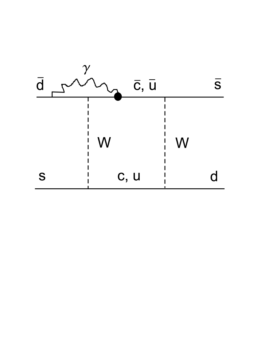
Figure 5: Diagram of T-odd radiation correction to the $K^{0}-\bar{K}^{0}$ mixing. Black circle denotes T-odd P-even vertex.

5 Conclusion

Thus, we have shown that besides P- T- odd electric dipole moment the particle can have T-violating P-conserving magnetic moment. We have considered the contribution of the T-odd magnetism to the P-odd T-even neutron-nucleus forward elastic scattering amplitude. We find, that the relative T-violation being of the order of unity corresponds to the T-odd P-even cross section (Fig. 3) being about of $10^{-2}-10^{-3}~{}mbarn$ in the energy region of $50~{}MeV-3~{}GeV$. The measurements for 12 MeV neutrons and ${}^{165}\mbox{Ho}$ target give the constraint of $10^{-2}~{}mb$ on five fold correlation cross section huf0 . If we relate this constraint to our energy range we find that $\mu_{T}\leq 1$.

It seems neutron EDM gives constraint $\mu_{T}\leq 0.1$.

Electrons and constituent quarks, in principle can possess T-violating P-conserving moments too. The way to search these may be the observation of forbidden decay modes of positronium-like systems from the ${}^{3}P_{1}$ and ${}^{1}P_{1}$ states.

6 Acknowledgment

The author is grateful to the Prof. V.G. Baryshevsky, Dr. K. Batrakov and Dr. D.Matsykevich for discussions and remarks.

References

- (1) A. Angelopoulos, A.Apostolakis, E.Aslanides et al., Phys. Lett. B 444, (1998) 43 .
- (2) V.G.Baryshevsky, Yad. Fiz. 38, (1983) 1162 (Sov. J. Nucl. Phys. 38, 699 ).
- (3) H.E.Conzett, Phys. Rev. C 48, (1993) 423.
- (4) M.Beyer, Nucl. Phys. A 560, (1993) 895 .
- (5) S.L.Cherkas, Nucl. Phys. A 671, (2000) 461.
- (6) J.E. Koster, E.D.Davis, C.R.Gould et al., Phys. Lett. B 267, (1991) 267.
- (7) P.R.Huffman et al., Phys.Rev. C 55, (1997) 2684.
- (8) F. Hinterberger, nucl-ex/9810003.
- (9) M. Simonius, Phys.Rev.Lett. 78, (1997) 4161.
- (10) N.R.Lipshutz, Phys. Rev. 158, (1967) 1491.
- (11) A.H.Huffman, Phys. Rev. D 1, (1970) 882.
- (12) V. B. Berestetskii, E. M. Lifshitz and L. P. Pitaevskii, Quantum Electrodynamics. Pergamon Press, Oxford 1982.
- (13) R.J.Blin-Stoyle, Fundamental interaction and the nucleus. Elsevier, Amsterdam 1973.
- (14) L.D.Landau and E. M. Lifshitz, Quantum mechanics. Pergamon Press, Oxford 1977.
- (15) The most easier to deduce (4) from Klein-Gordon equation: Substituting we find So we can rely on the equation (4) takes into account spin-less part of strong interaction correctly with accuracy
- (16) W.C Haxton, A.Hoering and M.J.Musolf, Phys. Rev. D50, (1994) 3422.
- (17) E.Leader and E.Predazzi, An introduction to gauge theories and the new physics, Cambrige university press 1982.
- (18) Particle Data Group, Eur. Phys. Jour. C15, (2000) 1.