On the size of hadrons

Abstract

The form factor and the mean-square radius of the pion are calculated analytically from a parametrized form of a $q\bar{q}$ wave function. The numerical wave function was obtained previously by solving numerically an eigenvalue equation for the pion in a particular model. The analytical formulas are of more general interest than just be valid for the pion and can be generalized to the case with unequal quark masses. Two different parametrizations are investigated. Because of the highly relativistic problem, noticable deviations from a non-relativistic formula are obtained.

1 Introduction

Hadrons are composite particles and therefore have a size. A quantitative measure of this size is the mean-square radius whose experimental value for the pion ($\pi^{+}$) is [1] $\sqrt{<r^{2}>}=0.67\pm 0.02$ fm. One determines it by first measuring the electro-magnetic form factor $F(Q^{2})$ for sufficiently small values of the (Feynman-four-) momentum transfer $Q^{2}=-(p_{e}-p_{e^{\prime}})^{2}$, and then taking the derivative at sufficiently small $Q^{2}$, i.e.

$$<r^{2}>=\left.-6\ \frac{dF(Q^{2})}{dQ^{2}}\right|_{Q^{2}=0}.$$ (1)

The form factor can also be calculated. One of the most remarkable simplicities of the light-cone formalism is that one can write down exact expressions for the electro-magnetic form factors. As was first shown by Drell and Yan [2], it is advantageous to choose a special coordinate frame to compute form factors and other current matrix elements at space-like photon momentum. In the Drell frame [3], the photon’s momentum is transverse to the momentum of the incident hadron and the incident hadron can be directed along the $z$ direction. With such a choice the four-momentum transfer is $-q_{\mu}q^{\mu}\equiv Q^{2}=\vec{q}_{\!\perp}^{\;2}$, and the quark current can neither create pairs nor annihilate the vacuum [4]. The space-like form factor for a hadron is just a sum of overlap integrals analogous to the corresponding non-relativistic formula [2]:

$$F_{S\rightarrow S^{\prime}}(Q^{2}) = \sum_{n}\sum_{f}e_{f}\int d[\mu_{n}]\,\Psi_{n,S^{\prime}}^{\star}(x_{i},\vec{\ell}_{\perp}{}_{i},\lambda_{i})\,\Psi_{n,S}(x_{i},\vec{k}_{\perp}{}_{i},\lambda_{i}),$$ (2)

$$\mathrm{with}\quad\vec{\ell}_{\!\perp i} \equiv \cases{\vec{k}_{\!\perp i}-x_{i}\vec{q}_{\!\perp}+\vec{q}_{\!\perp},&\hbox{for the struck quark,}\cr\vec{k}_{\!\perp i}-x_{i}\vec{q}_{\!\perp},&\hbox{for all other partons.}\cr}$$

The $d[\mu_{n}]$ symbolize the convolution over all momentum and helicity space arguments of every $\Psi_{n}$ and $e_{f}$ is the charge of the struck quark. This holds for any (composite) hadron and any initial or final spins $S$, but is particularly simple for a spin-zero hadron like a pion. The wave functions $\Psi_{n}=\Psi_{q\bar{q}},\Psi_{q\bar{q}g},\dots$ are the Fock-space projections of the eigenstate which for a meson for example are $|\Psi_{meson}\rangle=\sum_{i}(\Psi_{q\bar{q}}(x_{i},\vec{k}_{\!\perp_{i}},\lambda_{i})|q\bar{q}\rangle+\Psi_{q\bar{q}g}(x_{i},\vec{k}_{\!\perp_{i}},\lambda_{i})|q\bar{q}g\rangle+\dots)$. Their computation is the aim of the light-cone approach to the bound-state problem in gauge theory [4], by solving $H_{LC}|\Psi\rangle=M^{2}|\Psi\rangle$, with the eigenvalues $M^{2}$ being the invariant mass-squares of the physical mesons.

Strictly speaking, the above expression for the form factor contains contributions from all Fock space sectors. In this work, we restrict ourselves to the lowest Fock space projection consisting of a $q{\bar{q}}$ pair. There exists a nonzero probability of finding the pion in its valence state, which can be calculated [5]. It is known empirically, that the form factor at low $Q^{2}$ has essentially monopole structure [1]. The mean-square radius is essentially all the information there is for low $Q^{2}$. In fact, for the nucleon also, there are various effective three quark light-cone descriptions. In these models, without an explicit form of the effective potential in the light-cone Hamiltonian for three-quarks, one proceeds with an ansatz for the momentum space wave function. Both exponential [4] and power law [6, 4] falloff of this wave function at large $k_{\perp}$ have been used. The low $Q^{2}$ properties of the nucleon like the proton magnetic moment $\mu_{p}$ and its axial coupling $g_{A}$ have been investigated in these models [4]. It is reasonable to assume that the contributions from the higher Fock components will only refine this initial approximation [7].

We take the starting expression as,

$$F(Q^{2})=\!\!\int\!\!dx\,d^{2}\vec{k}_{\!\perp}\!\!\left(e_{1}\psi(x,\vec{k}_{\!\perp}+(1-x)\vec{q}_{\!\perp})+e_{2}\psi(x,\vec{k}_{\!\perp}-x\vec{q}_{\!\perp})\right)\psi(x,\vec{k}_{\!\perp}),$$ (3)

for the purpose of calculating its theoretical mean-square radius.

The relation involves only the $L_{z}=S_{z}=0$ component of the general $u\bar{d}$ wave function, where $\psi(x,\vec{k}_{\!\perp})\equiv\Psi_{u\bar{d}}(x,\vec{k}_{\!\perp};\uparrow\downarrow)$ is the (normalized) probability amplitude for finding the quarks with anti-parallel helicities, particularly for finding the $u$-quark with longitudinal momentum fraction $x$ and transversal momentum $\vec{k}_{\!\perp}$, and the $\bar{d}$ with $1-x$ and $-\vec{k}_{\!\perp}$. Their respective charges are $e_{1}$ and $e_{2}$, respectively, with $e_{1}+e_{2}=1$.

The $u\bar{d}$-component of the pion ($\pi^{+}$) is available in numerical form, since it has been computed recently in the $\uparrow\downarrow$-model [8]. But the three-dimensional numerical integration of Eq.(3) and it subsequent derivation with respect to $Q^{2}$ is cumbersome and may be numerically inaccurate. The aim of the present work is therefore to calculate the mean-square radius $<r^{2}>$ analytically by a suitable parametrization of the numerical wave function $\psi(x,\vec{k}_{\!\perp})$. The general procedure outlined in the subsequent sections is applicable also to more general cases.

2 General considerations

Usually, one is able to write down an integral equation in the three variables $x$ and $\vec{k}_{\!\perp}$ for the wavefunction $\psi(x,\vec{k}_{\!\perp})$ [8]. The solution of such an equation is numerically nontrivial, among other reasons, because the longitudinal momentum fractions are limited to $0\leq x\leq 1$. It is therefore advantageous to substitute the integration variable $x$ by another variable $-\infty\leq k_{z}\leq\infty$ which has the same range than either of the two transversal momenta $\vec{k}_{\!\perp}$. For unequal quark masses, the transformation is defined as,

$$x(k_{z})={E_{1}+k_{z}\over{E_{1}+E_{2}}}$$ (4)

with $E_{1,2}=\sqrt{{\bar{m}}_{1,2}+k_{\perp}^{2}+k_{z}^{2}}$. In the lowest order approximation, the effective quark masses ${\bar{m}}_{1,2}=m_{1,2}$.

For equal quark masses $m_{u}=m_{d}=m$, the substitution is so simple that it can even be inverted, i.e.

$$x(k_{z})=\frac{1}{2}\left(1+\frac{k_{z}}{\sqrt{m^{2}+\vec{k}_{\!\perp}^{\,2}+k_{z}^{2}}}\right)\quad\Longleftrightarrow\quad k_{z}^{2}=(m^{2}+\vec{k}_{\!\perp}^{\,2})\frac{(x-\frac{1}{2})^{2}}{x(1-x)}.$$ (5)

Formally, the three integration variables $k_{z}$ and $k_{\!\perp}$ look like a conventional 3-vector $\vec{p}\equiv(k_{z},\vec{k}_{\!\perp})$. If one substitutes, in addition, the unknown function $\psi(x,\vec{k}_{\!\perp})$ by an other unknown function $\varphi(\vec{p})$ according to

$$\psi(x,\vec{k}_{\!\perp})=\varphi(k_{z},\vec{k}_{\!\perp})\ \frac{N}{\sqrt{x(1-x)}}{\left(1+\frac{\vec{p}^{\;2}}{m^{2}}\right)^{\frac{1}{2}}},$$ (6)

one gets an identical integral equation in the three variables $\vec{p}$, which looks like an integral equation in usual momentum space. In the $\uparrow\downarrow$-model [8], the integral equation is further simplified and at the end looks very simple indeed,

$$M^{2}\varphi(\vec{p}) = \left[4m^{2}+4\vec{p}^{\,2}\right]\varphi(\vec{p})$$

$$- \frac{4}{3}\alpha\ \frac{1}{2\pi^{2}}\int\frac{d^{3}\vec{p}\,^{\prime}}{m}\left(\frac{4m^{2}}{(\vec{p}-\vec{p}\,^{\prime})^{\,2}}+\frac{2\mu^{2}}{\mu^{2}+(\vec{p}-\vec{p}\,^{\prime})^{2}}\right)\varphi(\vec{p}\,^{\prime}).$$

The equation was solved numerically in [8] for spherical symmetry $\varphi(\vec{p})=\varphi(p)$ and for the parameter values $m=1.16$, $\mu=3.8$, and $\alpha=0.6904$, where masses (and momenta) are expressed in units of $T=350\ \mathrm{MeV}$. The calculated eigenvalue for the ground state agrees with the pion mass-squared to a high degree of accuracy, and is stable with respect to changes in $\mu$ (renormalization). As can be seen from Fig. 2, it behaves like a power law $\varphi(p)\sim(1+(p/p_{a})^{2})^{-\kappa}$, rather than as anticipated in [3] like a Gaussian $\varphi(p)\sim\exp(-(p/p_{g})^{2})$. As shown in Appendix. A, a value of $\kappa=2$ is more likely than others and a fit of $p_{a}$,

$$\varphi(p)=\left(\frac{1}{1+p^{2}/p_{a}^{2}}\right)^{2},\qquad p_{a}=1.471,$$ (7)

reproduces the numerical wave function quite well as shown in Fig. 2, with albeit a comparatively large Bohr momentum $p_{a}$. Expressing the latter in a length, the value of $\sqrt{3}/p_{a}=0.66$ fm (similar to the experimental rms) is no numerical co-incidence, but the result of a constraint on the procedure in [8].

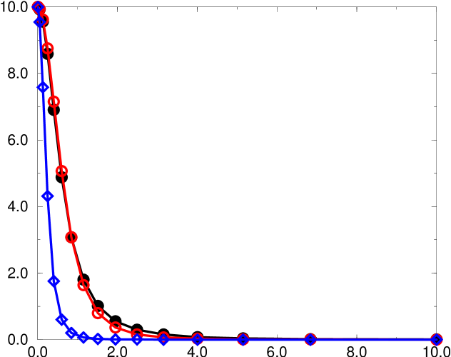
Figure 1: The pion wave function $\Phi(p)$ is plotted versus $p/(1.552\kappa)$ in an arbitrary normalization. The filled circles indicate the numerical results, the open circles the fit function. The diamonds denote the pure Coulomb solution.

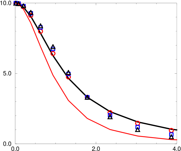
Figure 2: The function $\chi(p)$ is plotted versus p and fitted to the three exponents $\kappa=2,\frac{3}{2},1$ (triangle,box,circle). To guide the eye, $\varphi$ is included by the dotted line. Note the increased scale as compared to the left.

One should emphasize that only $\psi(x,\vec{k}_{\!\perp})$ but not $\varphi(p)=\varphi(x,\vec{k}_{\!\perp})$ is a probability amplitude, and that the two can differ appreciably from each other according to Eq.(6), particularly for a large Bohr momentum $p_{a}\sim m$ as in Eq.(7). Disregarding this proviso, and mistaking $\varphi(p)$ as a probability amplitude for finding the particle with relative momentum $p$, the calculation of the rms-radius would be trivial: One takes the Fourier transform of Eq.(7), i.e. $\mbox{FT}[\varphi(p)]\simeq\exp{(-p_{a}r)}$, and calculates its second moment to be

$$<r^{2}>_{FT}=\frac{\int dr\,r^{4}\,\exp{(-2p_{a}r)}}{\int dr\,r^{2}\,\exp{(-2p_{a}r)}}=\frac{3}{p_{a}^{2}}.$$

However, as the variable conjugate to the relative momentum $p$, the quantity $r$ is the relative distance of the particles. It is not the radius-distance from the common center-of-mass, with respect to which the rms is usually calculated. The latter is $r/2$ for equal mass particles, thus

$$<r^{2}>_{nr}=\frac{<r^{2}>_{FT}}{4}=\frac{3}{4p_{a}^{2}}.$$ (8)

It will be referred to as the ‘non-relativistic estimate’, since the above construction holds approximately if $k_{z}^{2}\ll m^{2}$ and $k_{\!\perp}^{\;2}\ll m^{2}$, thus $x\sim\frac{1}{2}$ according to Eq.(5). The question we pursue in the present work is thus: How large is the discrepancy between the non-relativistic estimate of Eq.(8) and the quasi-exact form factor according to Eq.(3) and its behaviour for low $Q^{2}$ according to Eq.(1), particularly for large Bohr momenta.

Before proceeding with the computation of the form factor, a number of notational definitions will be introduced, in terms of which the final results turn out to be simple. Once one has $\varphi(\vec{p})$ in a parametrized form like Eq.(7) one can transform back to the variables $x$ and $\vec{k}_{\!\perp}$. Since $\vec{p}^{\;2}\equiv k_{z}^{2}+\vec{k}_{\!\perp}^{\;2}$ one can use Eq.(5) to get

$$1+\frac{p^{2}}{p_{a}^{2}}=1+s^{2}\frac{(x-\frac{1}{2})^{2}}{x(1-x)}+\frac{s^{2}}{4m^{2}}\frac{\vec{k}_{\!\perp}^{\,2}}{x(1-x)}\equiv Z(x,\vec{k}_{\!\perp}^{\,2}).$$ (9)

The dimensionless variable $s$ is introduced conveniently as

$$s=\frac{m}{p_{a}},$$ (10)

as well as the isolation of the pure $x$-dependence by

$$X(x)\equiv 1+s^{2}\frac{(x-\frac{1}{2})^{2}}{x(1-x)}.$$ (11)

The combination $1+p^{2}/m^{2}$ is then trivially obtained by $s=1$. One can thus compute the form factor according to Eq.(3), i.e.

$$F(q_{\!\perp}^{2}) = \int dx\,dk_{\!\perp}^{2}\,|\psi(x,\vec{k}_{\!\perp})|^{2}\,f(x,k_{\!\perp};q_{\!\perp}),$$ (12)

$$<r^{2}> = \int dx\,dk_{\!\perp}^{2}\,|\psi(x,\vec{k}_{\!\perp})|^{2}\,g(x,k_{\!\perp}).$$ (13)

The function $f(x,k_{\!\perp};q_{\!\perp})$ and $g(x,k_{\!\perp})$ contain all the difficulty in the problem,

$$f(x,k_{\!\perp};q_{\!\perp}) = \int\limits_{0}^{2\pi}d\phi\ \frac{e_{1}\psi(x,\vec{k}_{\!\perp}+(1-x)\vec{q}_{\!\perp})+e_{2}\psi(x,\vec{k}_{\!\perp}-x\vec{q}_{\!\perp})}{2\,\psi(x,\vec{k}_{\!\perp})},$$ (14)

$$g(x,k_{\!\perp}) = -6\left.\displaystyle\dot{f}(x,k_{\!\perp};q_{\!\perp})\right|_{q_{\!\perp}=0}=-6\left.\displaystyle\frac{d}{dq_{\!\perp}^{2}}f(x,k_{\!\perp};q_{\!\perp})\right|_{q_{\!\perp}=0},$$ (15)

that is the integration over the angle $\phi$ between $\vec{k}_{\!\perp}$ and $\vec{q}_{\!\perp}$ ($\vec{k}_{\!\perp}\vec{q}_{\!\perp}=k_{\!\perp}q_{\!\perp}\cos\phi$). Finally the size parameter is introduced,

$$S\equiv\frac{\sqrt{<r^{2}>_{cal}}}{\sqrt{<r^{2}>_{exp}}}=\frac{\sqrt{<r^{2}>_{cal}}}{0.67~{}\textrm{fm}},$$ (16)

as a dimensionless measure of the size.

3 The parametrization of the wave function

Since the quarks move highly relativistically ($p_{a}^{2}\gg m^{2}$) and one cannot disregard the factor $\sqrt{1+p^{2}/m^{2}}$ in Eq.(6). One way to account for that is to parametrize directly

$$\chi(p)\equiv\varphi(p)\sqrt{1+\frac{\vec{p}^{\;2}}{m^{2}}}=\left(1+\frac{\vec{p}^{\;2}}{p_{s}^{\;2}}\right)^{-\kappa},$$ (17)

with the two adjustable parameters $\kappa$ and $p_{s}$. We have performed two fits, for two fixed values of $\kappa$, and have calculated analytically the size parameter $S$ according to Eq.(16). The results are:

$$\kappa=2,$$

One needs to consider essentially the integral

$$1=\int dxd^{2}\vec{k}_{\!\perp}|\psi(x,\vec{k}_{\!\perp})|^{2}\quad.$$

Inserting $\psi$ according to Eqs.(6) and (17) gives with $s=m/p_{s}$

$$\frac{1}{N^{2}} = \int\limits_{0}^{1}\frac{dx}{x(1-x)}\int\limits_{0}^{\infty}dk_{\!\perp}^{\,2}\int\limits_{0}^{2\pi}\frac{d\phi}{2}\ \frac{1}{\left[Z(x,\vec{k}_{\!\perp}^{\,2})\right]^{2\kappa}}.$$

The integration over $\phi$ is trivial, and the integration over $k_{\!\perp}^{\,2}$ elementary, since

$$\int\limits_{0}^{\infty}\frac{dk_{\!\perp}^{\,2}}{\left[Z(x,\vec{k}_{\!\perp}^{\,2})\right]^{\,n}}=\frac{4p_{s}^{2}x(1-x)}{(n-1)\left[X(x)\right]^{n-1}},$$ (18)

with $X(x)$ defined in Eq.(11). Introducing

$$A(s)=\int\limits_{0}^{1}dx\frac{1}{\left[X(x)\right]^{2\kappa-1}},$$

by definition, one remains with

$$\frac{1}{N^{2}}=\frac{4\pi p_{s}^{2}}{2\kappa-1}A(s).$$ (19)

Here the matter rests, since $A$ cannot be integrated in closed form.

For to compute the means-square radius, we first evaluate the function $f$ as defined in Eq.(14). In the general case one gets

$$f(x,k_{\!\perp};q_{\!\perp}) = \frac{e_{1}}{2}Z^{\kappa}\int\limits_{0}^{2\pi}d\phi\ \left[1+\displaystyle s^{2}\frac{(x-\frac{1}{2})^{2}}{x(1-x)}+\frac{\left(\vec{k}_{\!\perp}-(1-x)\vec{q}_{\!\perp}\right)^{\,2}}{4p_{s}^{2}x(1-x)}\right]^{-\kappa}$$

$$+ \frac{e_{2}}{2}Z^{\kappa}\int\limits_{0}^{2\pi}d\phi\ \left[1+\displaystyle s^{2}\frac{(x-\frac{1}{2})^{2}}{x(1-x)}+\frac{\left(\vec{k}_{\!\perp}-x\vec{q}_{\!\perp}\right)^{\,2}}{4p_{s}^{2}x(1-x)}\right]^{-\kappa}.$$

Using the abbreviative coefficient functions depending on $x$ and $k_{\!\perp}^{\,2}$, i.e.

$$b_{1}=Z+\frac{1-x}{x}\ \frac{q_{\!\perp}^{\,2}}{4p_{s}^{2}},\hskip 30.00005ptc_{1}=-\frac{1}{x}\frac{k_{\!\perp}}{p_{s}}\frac{q_{\!\perp}}{2p_{s}},$$ (20)

$$\dot{b}_{1}=\frac{1}{4\ p_{s}^{2}}\ \frac{1-x}{x},\hskip 40.00006ptc_{1}\dot{c}_{1}=\frac{1}{2\ p_{s}^{2}}\ \frac{1-x}{x}\ (Z-X),$$ (21)

and correspondingly $b_{2},c_{2},\dot{b}_{2}$ and $\dot{c}_{2}$ by exchanging $x\leftrightarrow 1-x$, gives

$$f(x,k_{\!\perp};q_{\!\perp})=Z^{\kappa}\int\limits_{0}^{\pi}d\phi\ \left[\frac{e_{1}}{\left(b_{1}+c_{1}\cos\phi\right)^{\kappa}}+\frac{e_{2}}{\left(b_{2}+c_{2}\cos\phi\right)^{\kappa}}\right].$$

The integration over $\phi$ can not be carried out in closed form for general values of $\kappa$.

3.1 The integrals for $\kappa=2$

The normalization integral is now

$$\frac{1}{N^{2}}=\frac{4\pi}{3}p_{s}^{2}A(s).$$

The contribution to $f$ from the up-quark becomes to leading order in $c$

$$\frac{\dot{f}}{f}=\frac{\dot{b}}{b}-3\frac{b\dot{b}-c\dot{c}}{b^{2}-c^{2}}\simeq-2\frac{\dot{b}}{b}+3\frac{c\dot{c}}{b^{2}}.$$

Inserting this into the definition of $g$ in Eq.(15) gives

$$g(x,k_{\!\perp})=\frac{3\pi}{x(1-x)p_{s}^{2}}\left[-\frac{2}{Z}+\frac{3X}{Z^{2}}\right]x^{2}.$$

Here we have taken both the quark and antiquark contributions (see Appendix B).

With the elementary $k_{\!\perp}^{2}$-integration of Eq.(18), one ends up with

$$<r^{2}>=\frac{6\pi}{5}N^{2}\int\limits_{0}^{1}\frac{dx}{x(1-x)}\frac{x^{2}}{\left[X(x)\right]^{4}}=\frac{9}{10p_{s}^{2}}\frac{R(s)}{A(s)}.$$

The two elementary integrals $A$ and $R$ are complicated but straightforward and yield

$$A(s) = \int\limits_{0}^{1}dx\frac{1}{\left[X(x)\right]^{3}}=\frac{-8-10s^{2}+3s^{4}+3b(s)s^{2}\left(8-4s^{2}+s^{4})\right)}{8(s^{2}-1)^{3}},$$

$$R(s) = \int\limits_{0}^{1}\frac{dx}{x(1-x)}\frac{x^{2}}{\left[X(x)\right]^{4}}=\frac{-136+72s^{2}-56s^{4}+15s^{6}}{48(s^{2}-1)^{4}}$$

$$\hskip 60.00009pt+3b(s)\ \frac{32-16s^{2}+36s^{4}-22s^{6}+5s^{8}}{48(s^{2}-1)^{4}}.$$

The auxiliary function $b(s)$ is an abbreviation for

$$b(s)=\frac{\mathrm{arctan}(\sqrt{s^{2}-1})}{\phantom{\mathrm{arctan}(}\sqrt{s^{2}-1}}.$$ (22)

The functions are plotted in Fig. 4.

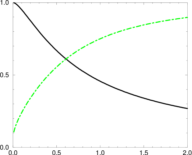
Figure 3: For $\kappa=2$, the functions $A(s)$ and $<r^{2}>$ (in units of ${3\over 4p_{s}^{2}})$ are plotted versus $s$ by the solid and the dashed-dotted line, respectively.

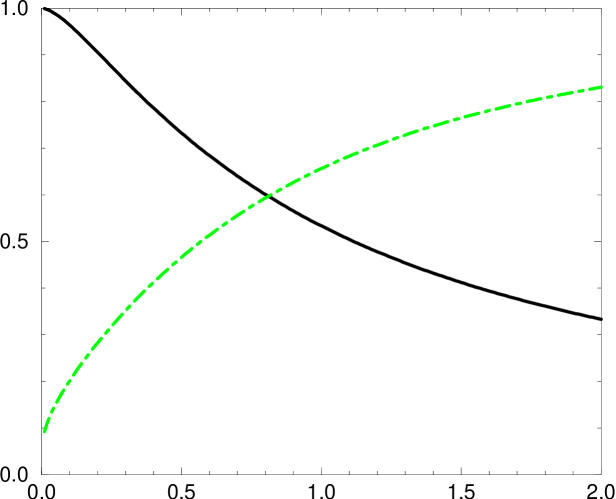
Figure 4: For $\kappa=\frac{3}{2}$, the functions $A(s)$ and $<r^{2}>$ (in units of ${3\over{4p_{s}^{2}}})$ are plotted versus $s$ by the solid and the dashed-dotted line, respectively.

As seen there, the asymptotic behaviour for $s\longrightarrow\infty$,

$$A(s)\rightarrow\frac{3\pi}{16s},\qquad R(s)\rightarrow\frac{5\pi}{32s},$$

is practically reached for values as small as $s=2$. Note that in the asymptotic limit $s\rightarrow\infty$, the mean-square radius reaches the correct non-relativistic value $<r^{2}>_{nr}=3/(4p^{2}_{s})$. As a final result, the size

$$S = \frac{\hbar c}{0.67\mbox{\,fm\,}T}\frac{s}{m}\ \sqrt{\displaystyle\frac{9R(s)}{10A(s)}}=\frac{0.8401}{m}\ s\ \sqrt{\displaystyle\frac{9R(s)}{10A(s)}},$$

is plotted in Fig. 6 for the mass value $m=1.16$ as function of $s$.

Figure 5: The root-mean-square radius of the pion, (i.e. $\sqrt{<r^{2}>}/0.67$ fm), is plotted versus $s$ by the solid line for $\kappa=2$ and by the dashed line for $\kappa=\frac{3}{2}$.

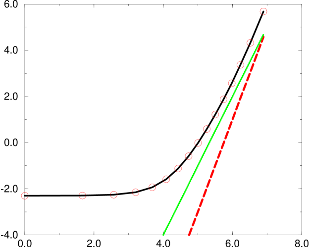
Figure 6: $\ln{1/\varphi}$ is plotted versus $\ln{p}$ (circle), and compared with $4\ln{p}$ (dashed) and $3\ln{p}$ (dotted line).

3.2 The case $\kappa=\frac{3}{2}$

According to Eq.(19), the normalization integral is for $\kappa=\frac{3}{2}$

$$\frac{1}{N^{2}}=2\pi p_{s}^{2}A(s).$$

In leading order in $c$, the contribution to the rms from the up-quark becomes

$$\frac{\dot{f}}{f}=-\frac{3}{2}\frac{\dot{b}}{b}+\frac{15}{8}\frac{c\dot{c}}{b^{2}}.$$

Inserting the derivatives from Eq.(21) gives (see Appendix C)

$$g(x,k_{\!\perp})=\frac{3\pi}{8p_{s}^{2}\,x(1-x)}\left[-\frac{9}{Z}+\frac{15X}{Z^{2}}\right]x^{2}.$$

With the elementary $k_{\!\perp}^{2}$-integration of Eq.(18), one ends up with

$$<r^{2}>=\frac{9\pi}{8}N^{2}\int\limits_{0}^{1}\frac{dx}{x(1-x)}\frac{x^{2}}{\left[X(x)\right]^{3}}=\frac{9}{16p_{s}^{2}}\frac{R(s)}{A(s)},$$

according to Eqs.(19) and (13). The elementary integrals are now

$$A(s) = \int\limits_{0}^{1}dx\frac{1}{\left[X(x)\right]^{2}}=\frac{2+s^{2}+b(s)s^{2}\left(-4+s^{2}\right)}{2(s^{2}-1)^{2}},$$

$$R(s) = \int\limits_{0}^{1}\frac{dx}{x(1-x)}\frac{x^{2}}{\left[X(x)\right]^{3}}=\frac{-20-8s^{2}+3s^{4}}{8(s^{2}-1)^{3}}$$

$$\hskip 60.00009pt+\ b(s)\ \frac{-16+8s^{2}+10s^{4}+3s^{6}}{8(s^{2}-1)^{3}}.$$

The auxiliary function $b(s)$ is the same as in Eq.(22). The functions are plotted in Fig. 4. Finally, the size function

$$S = \frac{\hbar c}{0.67\mbox{\,fm\,}T}\frac{s}{m}\ \sqrt{\displaystyle\frac{9R(s)}{16A(s)}}=\frac{0.8401}{m}\ s\ \sqrt{\displaystyle\frac{9R(s)}{16A(s)}}$$

is plotted in Fig. 6 for the mass value $m=1.16$ as function of $s$.

4 Summary and conclusion

We have analytically calculated the mean square radius for the pion in the light-cone approach in the valence sector. The contributions from the higher Fock space sectors are expected to only refine this initial approximation. We have used a parametrized form of the wave function in momentum space which had been obtained previously by solving the eigenvalue equation for the effective light-cone Hamiltonian. The mean square radius is calculated by first calculating the form factor at sufficiently low $Q^{2}$ and then taking its derivative with respect to $Q^{2}$ at $Q^{2}=0$. We have investigated two different values of the parametrization. $\kappa=2$ is found to be a better fit than $\kappa={3\over 2}$. We have shown that the mean square radius deviates noticably from the non-relativistic estimate because of the relativistic effects. In the asymptotic region (large $m^{2}$), it approaches the correct non-relativistic value.

5 Acknowledgement

AM would like to thank A. Harindranath for various useful discussions.

Appendix A The numerical wave function of the pion

The function $\varphi(p)$ was cumputed in previous work [9] and is tabulated in Table 1. It behaves much like an inverse power $\varphi(p)\sim(1+(p/p_{a})^{2})^{-\kappa}$. The value of $\kappa$ is closer to $2$ than to $\frac{3}{2}$, as demonstrated in Figure 6. Unfortunately, the maximum momentum of the Gaussian quadratures does not allow for a preciser statement.

Table 1: The calculated pion wave function $\varphi(p)$.

$p$	$\phi(p)$	$p$	$\phi(p)$
0.015739	10.00000	0.083241	9.928756
0.205995	9.563656	0.386376	8.592389
0.628023	6.908239	0.936173	4.877784
1.318156	3.077257	1.784203	1.801300
2.348743	1.011136	3.032468	0.554441
3.867276	0.297233	4.902437	0.154397
6.223861	0.076201	7.998102	0.034485
10.62105	0.013264	15.52088	0.003404

Appendix B The function $g(x,k_{\!\perp})$ for $\kappa=2$

Let us denote the contribution from the up-quark to the form factor function simply $f(x,k_{\!\perp};q_{\!\perp})$. For $\kappa=2$ one gets:

$$f(x,k_{\!\perp};q_{\!\perp})=Z^{2}\int\limits_{0}^{\pi}d\phi\ \frac{e}{\left(b+c\cos\phi\right)^{2}}=Z^{2}\pi e\frac{b}{\left(b^{2}-c^{2}\right)^{\frac{3}{2}}}.$$

Its derivative can be calculated quite in general

$$\frac{\dot{f}}{f}=\frac{\dot{b}}{b}-3\frac{b\dot{b}-c\dot{c}}{b^{2}-c^{2}}=\frac{\dot{b}(-2b^{2}+c^{2})+3bc\dot{c}}{b(b^{2}-c^{2})}.$$

In the limit $q_{\!\perp}\rightarrow 0$ (thus $c\rightarrow 0$) it becomes to leading order

$$\dot{f}=\left(-2\frac{\dot{b}}{b}+3\frac{c\dot{c}}{b^{2}}\right)\pi e.$$

Inserting the derivatives from Eq.(21) and taking the contributions from quark and anti-quark gives one gets thus with

$$g(x,k_{\!\perp})=\frac{3\pi}{p_{s}^{2}}\left[-\frac{2}{Z}+\frac{3X}{Z^{2}}\right]\left(e_{1}\frac{1-x}{x}+e_{2}\frac{x}{1-x}\right).$$

The expression in the round bracket has a contribution $(1-2x)$ which is odd under the exchange $x\leftrightarrow 1-x$,

$$e_{1}\frac{1-x}{x}+e_{2}\frac{x}{1-x}=\frac{\left[(e_{1}+e_{2})x^{2}+e_{1}(1-2x)\right]}{x(1-x)}\longmapsto\frac{(e_{1}+e_{2})x^{2}}{x(1-x)}.$$

It will vanish in the final integration over $x$ and can be omitted. This leaves one with the final expression

$$g(x,k_{\!\perp})=\frac{3\pi}{x(1-x)\ p_{s}^{2}}\left(e_{1}+e_{2}\right)\left[-\frac{2}{Z}+\frac{3X}{Z^{2}}\right]x^{2}.$$ (23)

Appendix C The function $g(x,k_{\!\perp})$ for $\kappa=\frac{3}{2}$

The form factor function for the up-quark

$$f=\int\limits_{0}^{\pi}d\phi\frac{eZ^{\frac{3}{2}}}{(b+c\,\textrm{cos}\phi)^{\frac{3}{2}}}=\frac{2eZ^{\frac{3}{2}}}{p}\mathrm{E}[q],\ \textrm{with}\ \cases{p=(b-c)\sqrt{(b+c)},&\cr q=\displaystyle\frac{2c}{b+c},&\cr}$$

can be integrated in closed form also for $\kappa={3}/{2}$ and be expressed in terms of the complete elliptic integrals of the second kind, $E[q]\equiv\int_{0}^{\frac{\pi}{2}}d\theta\sqrt{1-q\ \mathrm{sin}^{2}\theta}$. Since ${dE[q]}/{dq}=\left(E[q]-K[q]\right)/{2q}$, the derivative is

$$\frac{\dot{f}}{f}=\frac{\dot{q}}{q}\ \frac{E[q]-K[q]}{2E[q]}-\frac{\dot{p}}{p}.$$

Both derivatives $\dot{q}$ and $\dot{p}$ have a potentially dangerous singularity $b\dot{c}$,

$$\frac{\dot{q}}{q}=\frac{-c\dot{b}+b\dot{c}}{(b+c)c},\qquad\mbox{and}\qquad\frac{\dot{p}}{p}=\frac{(3b+c)\dot{b}-(3c+b)\dot{c}}{2(b^{2}-c^{2})}.$$

To cure the problem, one must expand

$$\frac{E[q]-K[q]}{E[q]}=-\frac{q}{2}-\frac{5q^{2}}{16}-\mathrm{O}[q^{3}]\simeq-\frac{c}{b+c}\left(1+\frac{5}{4}\frac{c}{b+c}\right),$$

to a sufficiently high order, which upon insertion yields

$$\frac{\dot{f}}{f} = \dot{b}\left[\frac{+c}{2(b+c)^{2}}\left(1+\frac{5c}{4(b+c)}\right)-\frac{3b+c}{2(b^{2}-c^{2})}\right]$$

$$+ \dot{c}\left[\frac{-b}{2(b+c)^{2}}\left(1+\frac{5c}{4(b+c)}\right)+\frac{b+3c}{2(b^{2}-c^{2})}\right].$$

The leading terms in the coefficient of $\dot{c}$ now tend to cancel, i.e.

$$\frac{\dot{f}}{f} = \dot{b}\left[\frac{+c}{2(b+c)^{2}}\left(1+\frac{5c}{4(b+c)}\right)-\frac{3b+c}{2(b^{2}-c^{2})}\right]$$

$$+ \frac{c\dot{c}}{b+c}\left[\frac{-5b}{8(b+c)^{2}}+\frac{3}{2(b-c)}+\frac{b}{(b^{2}-c^{2})}\right]\longrightarrow-\frac{3}{2}\frac{\dot{b}}{b}+\frac{15}{8}\frac{c\dot{c}}{b^{2}}.$$

In the last step only terms were kept which survive in the limit $c\rightarrow 0$. Inserting the derivatives from Eq.(21) gives for the complete amplitude

$$g(x,k_{\!\perp})=\frac{3\pi}{8x(1-x)p_{s}^{2}}\left(e_{1}+e_{2}\right)\left[-\frac{9}{Z}+\frac{15X}{Z^{2}}\right]x^{2},$$ (24)

where the same simplifications have been done as in the previous section.

References

[1]
S.R. Amendolia et al.,
Phys. Lett. 146B (1984) 116.
[2]
S.D. Drell and T.M. Yan,
Phys. Rev. Lett. 24 (1970) 181.
[7] R. J. Perry, A. Harindranath and K. G. Wilson, Phys. Rev.
Lett. 65 (1991) 4051.
[8]
H.C. Pauli,
in: New directions in Quantum Chromodynamics,
C.R. Ji and D.P. Min, Eds.,
American Institute of Physics, 1999, p. 80-139.
hep-ph/9910203.