Massive fermion production in nonsingular superstring cosmology

Abstract

We study massive spin-1/2 fermion production in nonsingular superstring cosmology, taking into account one-loop quantum corrections to a superstring effective action with dilaton and modulus fields. While no creation occurs in the massless limit, massive fermions can be produced by the existence of a time-dependent frequency. Due to the increase of the Hubble expansion rate during the modulus-driven phase, the occupation of number of fermions continues to grow until the point of the graceful exit, after which fermion creation ceases with the decrease of the Hubble rate.

]

I Introduction

With the development of superstring theory, string-inspired cosmological models [1] have received much attention to describe the evolution of the very early stage of the Universe. Most of such scenarios are based on the low-energy effective field theory, which is expected to be valid at the Planck scale. While a full theory is not yet established, it is important to test the viability of string theories by extracting various cosmological implications from them.

Among string-motivated cosmological models proposed so far, the pre-big-bang (PBB) scenario [2] has been most widely studied. If one assumes that the Universe has a $T$-duality, there exist two disconnected branches. One of which ($t<0$) corresponds to the stage of superinflation driven by the kinetic term of the dilaton field, and another ($t>0$) is the Friedmann branch where the Universe exhibits standard decelerating expansion. The PBB scenario basically requires the existence of nonsingular solutions which interpolates between two disconnected branches [3]. In the tree-level superstring action, however, one has no-go results that singularity can not be avoided [4, 5].

In order to overcome such singularity problems, Antoniadis, Rizos, and Tamvakis [6] involved one-loop quantum corrections to the string effective action with dilaton and modulus fields, and found some nonsingular solutions. Since the success of singularity avoidance is mainly determined by the motion of the modulus field, the allowed ranges of parameters have been analyzed in the absence of the dilaton field in the flat Friedmann-Robertson-Walker (FRW) background [7] and the anisotropic Bianchi type-I metric [8]. In the full dilaton-modulus system, several authors studied generality of singularity avoidance in the closed FRW [9] and Bianchi type-I and -IX [10] spacetimes. It was found that nonsingular solutions generically exist except for the Bianchi-IX case.

From observational point of view, analysis of the perturbations predicted in the PBB model is an important issue in order to test realistic string theories. In this respect, many authors investigated quantum creation of scalar particles such as dilaton and axions [11, 12, 13, 14, 15, 16], and production of gravitational waves [17, 18, 19], most of which exhibit different spectra compared to the standard cosmology. Another interesting prediction in the PBB scenario is the generation of primordial magnetic fields due to the break of the conformal invariance [20, 21].

Recently, Brustein and Hadad [22] studied fermion production in superstring cosmology in the presence of the dilaton coupling only. It was found that massless fermions are not created, since the equation of fermions reduces to that in the Minkowski spacetime in the massless limit. In this Letter, we investigate massive fermion production in more general dilaton-modulus system whereby singularity can be avoided. In fact we will show that massive fermions are nonadiabatically created due to the existence of a time-dependent mass term.

II Nonsingular solutions

Consider the following one-loop effective action of the heterotic superstring theory [6, 9, 10],

$$S = \int d^{4}x\sqrt{-g}\Biggl{[}\frac{1}{2}R-\frac{1}{4}(\nabla\phi)^{2}-\frac{3}{4}(\nabla\sigma)^{2}$$ (1)

$$- \frac{1}{6}H_{\mu\nu\lambda}H^{\mu\nu\lambda}+\frac{1}{16}\left\{\lambda e^{\phi}-\delta\xi(\sigma)\right\}R_{\rm GB}^{2}\Biggr{]},$$ (2)

written in the Einstein frame. Here $R$, $\phi$, $\sigma$, and $H_{\mu\nu\lambda}$ are the scalar curvature, the dilaton, the modulus, and the antisymmetric tensor field, respectively. In this work we set $H_{\mu\nu\lambda}=0$ and neglect the curvature terms higher than the second order. The Gauss-Bonnet term, $R_{\rm GB}$, is defined as

$$R_{\rm GB}^{2}=R^{2}-4R^{\mu\nu}R_{\mu\nu}+R^{\mu\nu\alpha\beta}R_{\mu\nu\alpha\beta}.$$ (3)

In the presence of the last term in the action (2) (i.e, one-loop quantum corrections), singularity problems in the tree-level action can be avoided [6]. The coefficients, $\lambda$ and $\delta$, are determined by the inverse string tension $\alpha^{\prime}$ and the four-dimensional trace anomaly of the $N=2$ sector, respectively. While $\lambda$ is positive definite, $\delta$ can be either positive or negative.

The function, $\xi(\sigma)$, is expressed as

$$\xi(\sigma)={\rm ln}\left[2e^{\sigma-\pi e^{\sigma}/3}\left\{\prod_{n=1}^{\infty}\left(1-e^{-2n\pi e^{\sigma}}\right)\right\}^{4}\right].$$ (4)

Then the first derivative of $\xi(\sigma)$ in terms of $\sigma$ is well approximated as $\xi^{\prime}(\sigma)=-(2\pi/3)\sin{\rm h\sigma}$, which we use in our numerical analysis.

It is also convenient to introduce a dimensionless function, $f(\phi,\sigma)\equiv[e^{\phi}-\bar{\delta}\xi(\sigma)]/16$ with $\bar{\delta}\equiv\delta/\lambda$. We normalize time and spatial coordinates by the string length scale $\sqrt{\lambda}$ as $\bar{x^{\mu}}=x^{\mu}/\sqrt{\lambda}$, and scalar fields as $\bar{\phi}=\phi\sqrt{\lambda}$, $\bar{\sigma}=\sigma\sqrt{\lambda}$. Hereafter we drop bars for simplicity.

Adopting the flat FRW metric as the background spacetime, with $a\equiv e^{p}$ being the scale factor, the dynamical equations for the metric and scalar fields yield

$$8(1+8\dot{p}\dot{f})(\ddot{p}+\dot{p}^{2})+4(1+8\ddot{f})\dot{p}^{2}+\dot{\phi}^{2}+3\dot{\sigma}^{2}=0,$$ (5)

$$\ddot{\phi}+3\dot{p}\dot{\phi}-2f_{,\phi}R^{2}_{\rm GB}=0,$$ (6)

$$\ddot{\sigma}+3\dot{p}\dot{\sigma}-\frac{2}{3}f_{,\sigma}R^{2}_{\rm GB}=0,$$ (7)

together with the constraint equation,

$$12\dot{p}^{2}+96\dot{p}^{3}\dot{f}-\dot{\phi}^{2}-3\dot{\sigma}^{2}=0.$$ (8)

Here an overdot denotes a derivative with respect to cosmic time, $t$, and the Gauss-Bonnet term is given as $R^{2}_{\rm GB}=24\dot{p}^{2}(\ddot{p}+\dot{p}^{2})$. Nonsingular cosmological solutions have been found for negative values of $\delta$ [6, 9].

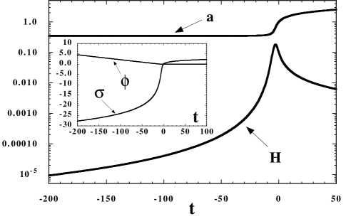
FIG. 1.: The evolution of the Hubble rate is plotted when the singularity is avoided. We choose $\delta=-48/\pi$, and set $\phi=\dot{\phi}=0$, $\sigma=0$, $p=0$ at $t=0$. $\dot{\sigma}$ is determined by the constraint equation (8) as $\dot{\sigma}=0.2$. Inset: $\phi$ and $\sigma$ vs $t$. The evolution of the system is dominated by the $\sigma$ field around the graceful exit.

In the absence of the modulus field, the scale factor in the Einstein frame evolves as $a\propto|t|^{1/3}$ during the dilaton-driven phase. For negative $t$, this corresponds to the accelerated contraction, $\dot{a}<0$ and $\ddot{a}<0$. In the tree-level action, one needs to assume that the epoch of the accelerated evolution comes to an end at some time in order to make a smooth transition to another branch ($t>0$). In the present scenario, however, taking into account one-loop corrections opens up the possibility of the graceful exit driven by the kinetic energy of the modulus field.

We show one nonsingular solution in Fig. 1. Generally the Hubble rate, $H\equiv\dot{p}$, grows as $H\propto(-t)^{-2}$ during the modulus-driven phase. In order to avoid singularity at $t=0$, the velocity of $\phi$ is required to be much smaller than $\sigma$ during the graceful exit. If $|\dot{\phi}|$ is sufficiently small around $t=0$, there always exist nonsingular solutions for $\phi<0$. This is because $e^{\phi}\approx 0$ for negative large values of $\phi$, which indicates that the singularity avoidance is practically independent of $\phi$. The allowed parameter regions with respect to $\phi$ were precisely analyzed in Ref. [10], which we do not repeat it here.

The sign of $\dot{\sigma}$ does not change during the whole evolution. For $\dot{\sigma}>0$ which corresponds to the case of Fig. 1, $\sigma$ rapidly moves relative to $\phi$ around the graceful exit. After a smooth transition at $t=0$, the dilaton freezes with $\phi\sim 0$ and the modulus evolves as $\sigma\propto{\rm ln}~{}t$ as $t\to\infty$. The Hubble rate begins to decrease for $t>0$, which asymptotically approaches the Friedmann-like Universe, $a\propto t^{1/3}$ and $H\sim 1/(3t)$.

III Massive fermion production

Let us consider the following action for the fermion field $\psi$ with bare mass $m$:

$$S_{\rm fermion}=\int d^{4}x\sqrt{-g}~{}f\left(i\bar{\psi}\bar{\gamma}^{\mu}\overrightarrow{D}_{\mu}\psi-m\bar{\psi}\psi\right),$$ (9)

where $\bar{\gamma}^{\mu}$ is the curved-space Dirac matrices, and $D_{\mu}\equiv\partial_{\mu}+(1/4)\gamma_{\alpha\beta}\omega_{\mu}^{\alpha\beta}$ is the spin-1/2 covariant derivative, where $\omega_{\mu}^{\alpha\beta}$ is the spin connection. $\gamma_{\alpha}$ denotes the Dirac matrices in Minkowski spacetime with $\gamma_{\alpha\beta}\equiv\gamma_{[\alpha}\gamma_{\beta]}$.

From the action (9) we obtain the Dirac equation,

$$\left(i\bar{\gamma}^{\mu}D_{\mu}-m+\frac{i}{2}\frac{\partial_{\mu}f}{f}\bar{\gamma}^{\mu}\right)\psi=0.$$ (10)

Since $\bar{\gamma}^{0}=\gamma^{0}$, $\bar{\gamma}^{i}=\gamma^{i}/a$, and $\bar{\gamma}^{\mu}D_{\mu}=\bar{\gamma}^{\mu}\partial_{\mu}+(3/2)H\gamma^{0}$ in the flat FRW background, Eq. (10) is simplified by introducing a new field, $\chi\equiv a^{3/2}f^{1/2}\psi$, as

$$\left(i\gamma^{\mu}\partial_{\mu}-ma\right)\chi=0,$$ (11)

where $\partial_{0}$ denotes the derivative with respect to conformal time, $\eta\equiv\int a^{-1}dt$. We decompose the $\chi$ field into Fourier modes as

$$\chi\left(x\right) = \int\frac{d^{3}k}{(2\pi)^{3/2}}e^{-i\vec{k}\cdot\vec{x}}$$ (12)

$$\times \sum_{s=\pm 1}\left[u_{s}(k,\eta)a_{s}(k)+v_{s}(k,\eta)b_{s}^{\dagger}(-k)\right],$$ (13)

where $v_{s}(k)=C{\bar{u}}^{T}_{s}(-k)$ with $C$ being a constant.

Defining $u_{s}=\left[u_{+}(\eta)\varphi_{s}(k),su_{-}(\eta)\varphi_{s}(k)\right]^{T}$ and $v_{s}=\left[sv_{+}(\eta)\varphi_{s}(k),v_{-}(\eta)\varphi_{s}(k)\right]^{T}$ with $\varphi_{s}(k)$ being eigenvectors of helicity operators, the Dirac equation (11) reads [23, 24]

$$u^{\prime}_{\pm}(\eta)=iku_{\mp}(\eta)\mp imau_{\pm}(\eta),$$ (14)

which reduces to the decoupled form:

$$u^{\prime\prime}_{\pm}+\left[\omega_{k}^{2}\pm i(ma)^{\prime}\right]u_{\pm}=0,$$ (15)

where $\omega_{k}^{2}\equiv k^{2}+(ma)^{2}$. Note that we imposed the normalization conditions, $u_{r}^{\dagger}(k,\eta)v_{s}(k,\eta)=0$, $u_{r}^{\dagger}(k,\eta)u_{s}(k,\eta)=v_{r}^{\dagger}(k,\eta)v_{s}(k,\eta)=\delta_{rs}$, $|u_{+}|^{2}+|u_{-}|^{2}=2$.

In order to diagonalize the Hamiltonian, we introduce new operators, ${\hat{a}}(k,\eta)=\alpha_{k}(\eta)a(k)+\beta_{k}(\eta)b^{\dagger}(-k)$ and ${\hat{b}}^{\dagger}(k,\eta)=-\beta^{*}_{k}(\eta)a(k)+\alpha^{*}_{k}(\eta)b^{\dagger}(-k)$, where the Bogolyubov coefficients satisfy

$$\alpha_{k}=\frac{E_{k}+\omega_{k}}{F^{*}_{k}}\beta_{k},~{}~{}|\beta_{k}|^{2}=\frac{|F_{k}|^{2}}{2\omega_{k}(\omega_{k}+E_{k})},$$ (16)

with

$$E_{k}=k{\rm Re}(u_{+}^{*}u_{-})+ma\left(1-|u_{+}|^{2}\right),$$ (17)

$$F_{k}=(k/2)\left(u_{+}^{2}-u_{-}^{2}\right)+mau_{+}u_{-}.$$ (18)

Note that the canonical commutation relation leads to $|\alpha_{k}|^{2}+|\beta_{k}|^{2}=1$, which restricts the occupation numbers of fermions as $n_{k}\equiv|\beta_{k}|^{2}\leq 1$. The initial conditions are chosen as $u_{\pm}(\eta_{0})=\sqrt{(\omega_{k}\mp ma)/\omega_{k}}$, corresponding to $E_{k}(\eta_{0})=\omega_{k}$, $F_{k}(\eta_{0})=0$, and $n_{k}(\eta_{0})=0$.

FIG. 2.: The evolution of the occupation number of fermions for three cases: $k=10^{-2},m=10^{-2}$; $k=10^{-1},m=1$; and $k=1,m=10^{-6}$, where $k$ and $m$ are normalized by the string length scale, $\sqrt{\lambda}$. The $\delta$ and initial values of background quantities are the same as in Fig. 1. The enhancement of fermions strongly depends on the relation of two parameters, $k$ and $m$.

In the limit of $m\to 0$, Eq. (15) reduces to that in Minkowski spacetime,

$$u^{\prime\prime}_{\pm}+k^{2}u_{\pm}=0.$$ (19)

The solution for this equation is expressed as $u_{\pm}(\eta)=e^{ik(\eta-\eta_{0})}$, where we used the initial conditions, $u_{\pm}(\eta_{0})=1$. Then we have $n_{k}=0$ by Eqs. (16)-(18), which indicates that no creation occurs in the massless limit [22].

When the mass of fermion is sufficiently small relative to the physical wave number ($m\ll k/a$), the situation is similar to the massless case. In Fig. 2 we find that fermions are hardly excited for $k=1$ and $m=10^{-6}$, where $k$ and $m$ are normalized by the string length scale, $\sqrt{\lambda}$. Note that the acquired number of e-foldings during the modulus-driven phase is not large compared to the standard inflationary scenarios, e.g., if we normalize the scale factor as $a=1$ for $t=0$, $a\approx 0.345$ for $t=-500$ at which the contribution of modulus begins to be important relative to dilaton. This indicates that when the condition, $m\ll k/a$, holds in the initial stage of the modulus-driven phase, it is typically valid even around the graceful exit.

FIG. 3.: The occupation number of fermions at the end of the modulus-driven phase as a function of the fermion mass, $m$, for three different comoving momenta, $k=10^{-4}$, $k=10^{-2}$, and $k=1$. The $\delta$ and initial values of background quantities are the same as in Fig. 1.

When $m$ and $k/a$ are comparable during the modulus-driven phase, massive fermions are created due to the existence of the time-dependent mass term in Eq. (15). In Fig. 2 the number density of fermions continues to grow until the point of the graceful exit for the cases of $k=10^{-2},m=10^{-2}$; and $k=10^{-1},m=1$. The nonadiabatic condition where particles are sufficiently excited can be written as $|\dot{\omega}_{k}|~{}\mbox{\raisebox{-4.30554pt}{$\stackrel{{\scriptstyle\textstyle>}}{{\textstyle\sim}}$}}~{}\omega_{k}^{2}$, which yields

$$H~{}\mbox{\raisebox{-4.30554pt}{$\stackrel{{\scriptstyle\textstyle>}}{{\textstyle\sim}}$}}~{}\frac{\left[k^{2}+(ma)^{2}\right]^{3/2}}{(ma)^{2}}.$$ (20)

In a dust or radiation dominated Universe, the Hubble rate decreases as $H\propto 1/t$, which works to violate the nonadiabatic condition, (20). In fact, in preheating after inflation, unless an inflaton decay to fermions is not taken into account, the mass term $(ma)^{2}$ does not lead to sufficient fermion production [23, 25, 26, 27]. However, in the present model, the growth of the Hubble rate during the modulus-driven phase assists the nonadiabatic condition to hold, which results in nonperturbative particle creation solely by the time-dependent mass term. The growth of the occupation number ends after the smooth transition to the Friedmann-like Universe, since the Hubble rate begins to decrease (see Fig. 1).

When $m$ is much larger than $k/a$, fermion production is generally suppressed. Especially for $m\gg H$ where the nonadiabatic condition (20) is not satisfied, Eq. (15) is approximately written as $\ddot{X}_{\pm}+m^{2}X_{\pm}\simeq 0$ with $X_{\pm}\equiv a^{1/2}u_{\pm}$. This indicates that fermions are hardly created in the supermassive limit, $m\to\infty$.

In Fig. 3 we plot the occupation number of fermions at $t=0$ as a function of mass for three different momenta. For each momentum, there exists a maximum $n_{k}$ for some value of $m$ ($=m_{*}$). Since $m_{*}$ is typically of the same order as the each corresponding momentum, the curves shift from left to right with increasing $k$. If the $1/\sqrt{\lambda}$ is around the Planck scale, our results suggest that massive fermions heavier than the GUT scale can be copiously produced, which may play important roles for the leptogenesis scenarios [23].

IV Conclusions and discussions

We have investigated the production of massive spin-1/2 fermions in nonsingular superstring cosmology with dilaton and modulus fields. The existence of the modulus coupled to the Gauss-Bonnet curvature invariant leads to a smooth transition from the modulus-driven accelerated expansion phase toward the Friedmann-like Universe. Since the Hubble rate increases before the graceful exit, this makes it possible to produce massive fermions in terms of nonadiabatic change of their frequencies. In particular, fermions are most efficiently excited when the bare mass $m$ is comparable to the physical momentum, $k/a$. In both massless and supermassive limits, fermion creation is strongly suppressed.

The occupation number of fermions achieved by the time-dependent mass term $(ma)^{2}$ is typically smaller than the Pauli bound, $n_{k}=1$, even at the end of the modulus-driven phase. If one introduces the Yukawa couplings between two scalar fields $\phi,\sigma$ and the fermion $\psi$ such as $h_{1}\phi\bar{\psi}\psi$ and $h_{2}\sigma\bar{\psi}\psi$, the effective mass of fermions is expressed as [27]

$$m_{\rm eff}=m+h_{1}\phi+h_{2}\sigma.$$ (21)

In this case it is known that particle creation is most efficient when $m_{\rm eff}$ vanishes, leading to $n_{k}\sim 1$ both in the context of inflation [24] and preheating [23, 25, 26, 27]. In the present scenario, since $m_{\rm eff}$ vanishes or becomes close to zero depending on two coupling constants, $h_{1}$ and $h_{2}$, this may further strengthen nonadiabatic amplification of fermions. We leave to future work about the precise investigation of this issue.

Although we have restricted ourselves in spin-1/2 fermions satisfying the Dirac equation, nonthermal production of gravitinos (spin-3/2 fermions) has recently become an issue of great importance [28]. Gravitinos have both helicity-3/2 and -1/2 states. While the helicity-3/2 mode reduces to the form of the Dirac equation, the helicity-1/2 mode behaves like the goldstino in global supersymmetric limit. It was shown in Ref. [22] that the latter mode also reduces to the same form as the former mode in the massless limit by assuming the power-law evolution of the scale factor in the standard PBB scenario, which means that creation of massless gravitinos is highly suppressed. However, the situation will change for massive gravitinos, in which case the existence of time-dependent mass terms may lead to the amplification of gravitinos during the modulus-driven phase. It is certainly of interest to study gravitino production in realistic nonsingular cosmology, since this provides a powerful mechanism to distinguish between different models of string theories and regions of the parameter space, together with the CMB constraint by scalar and tensor metric perturbations produced during the graceful exit [29].

ACKOWLEDGMENTS

We thank Bruce A. Bassett and Kei-ichi Maeda for useful discussions. This work was supported by the Waseda University Grant for Special Research Projects.

REFERENCES

- [1] J. E. Lidsey, D. Wands and E. J. Copeland, Phys. Rep. 337, 343 (2000).
- [2] G. Veneziano, Phys. Lett. B 265, 287 (1991); M. Gasperini and G. Veneziano, Astropart. Phys. 1, 317 (1993); Mod. Phys. Lett. A 8, 3701 (1993).
- [3] M. Gasperini and G. Veneziano, Phys. Lett. B 329, 429 (1994).
- [4] R. Easther, K. Maeda, and D. Wands, Phys. Rev. D 53, 4247 (1996);.
- [5] N. Kaloper, R. Madden, and K. A. Olive, Nucl. Phys. B452, 677 (1995); Phys. Lett. B 371, 34 (1996).
- [6] I. Antoniadis, J. Rizos, and K. Tamvakis, Nucl. Phys. B415, 497 (1994).
- [7] Rizos and Tamvakis, Phys. Lett. B 326, 57 (1994).
- [8] S. Kawai, M. Sakagami, and J. Soda, Phys. Lett. B 437, 284 (1998); S. Kawai and J. Soda, Phys. Rev. D 59, 063506 (1999).
- [9] R. Easther and K. Maeda, Phys. Rev. D 54, 7252 (1996).
- [10] H. Yajima, K. Maeda, and H. Ohkubo, Phys. Rev. D 62, 024020 (2000).
- [11] M. Gasperini and G. Veneziano, Phys. Rev. D 50, 2519 (1994).
- [12] E. J. Copeland, R. Easther, and D. Wands, Phys. Rev. D 56, 874 (1997).
- [13] R. Brustein and M. Hadad, Phys. Rev. D 57, 725 (1998).
- [14] R. Durrer, M. Gasperini, M. Sakellariadou, and G. Veneziano, Phys. Rev. D 59, 043511 (1999).
- [15] F. Vernizzi, A. Melchiorri, and R. Durrer, Phys. Rev. D 63, 063501 (2001).
- [16] R. Durrer, K. E. Kunze, and M. Sakellariadou, astro-ph/0010408 (2000).
- [17] R. Brustein, M. Gasperini, M. Giovannini and G. Veneziano, Phys. Lett. B 361, 45 (1995).
- [18] A. Buonanno, M. Maggiore, and C. Ungarelli, Phys. Rev. D 55, 3330 (1997).
- [19] C. Cartier, E. J. Copeland, and M. Gasperini, gr-qc/0101019 (2001).
- [20] M. Gasperini, M. Giovannini, and G. Veneziano, Phys. Rev. Lett. 75, 3796 (1995).
- [21] D. Lemoine and M. Lemoine, Phys. Rev. D 52, 1955 (1995).
- [22] R. Brustein and M. Hadad, Phys. Lett. B 477, 263 (2000).
- [23] G. F. Giudice, M. Peloso, A. Riotto, and I. I. Tkachev, JHEP 9908, 014 (1999); M. Peloso and L. Sorbo, JHEP 0005, 016 (2000).
- [24] D. Chung, E. Kolb, A. Riotto, and I. I. Tkachev, Phys. Rev. D 62, 043508 (2000).
- [25] J. Baacke, K. Heitman, and C. Patzold, Phys. Rev. D 58, 125013 (1998).
- [26] P. B. Greene and L. Kofman, Phys. Lett. B 448, 6 (1999); Phys. Rev. D 62, 123516 (2000).
- [27] S. Tsujikawa, B. A. Bassett, and F. Viniegra, JHEP 0008, 019 (2000).
- [28] A. L. Maroto and A. Mazumdar, Phys. Rev. Lett. 84, 1655 (2000); R. Kallosh, L. Kofman, A. Linde, and A. Van Proeyen, Phys. Rev. D 61, 103503 (2000); Class. Quant. Grav. 17, 4269 (2000); G. F. Giudice, I. I. Tkachev, and A. Riotto, JHEP 9908, 009 (1999); G. F. Giudice, A. Riotto, and I. I. Tkachev, JHEP 9911, 036 (1999); D. H. Lyth and H. B. Kim, hep-ph/0011262 (2000).
- [29] S. Kawai and J. Soda, Phys. Lett. B 460, 41 (1999).