On the effective light-cone QCD-Hamiltonian:
Application to the pion and other mesons

Abstract

The effective interaction between a quark and an anti-quark as obtained previously with by the method of iterated resolvents is replaced by the $\uparrow\downarrow$-model and applied to flavor off-diagonal mesons including the $\pi^{+}$. The only free parameters are the canonical ones, the coupling constant and the masses of the quarks.

The light-cone approach [1] to the bound-state problem in gauge theory [2] aims at solving $H_{LC}|\Psi\rangle=M^{2}|\Psi\rangle$. If one disregards possible zero modes [4] and works in the light-cone gauge, the (light-cone) Hamiltonian $H_{LC}$ is given as a Fock-space operator in [2], or in the compendium [3]. Its eigenvalues are the invariant mass-squares $M^{2}$ of physical particles associated with the eigenstates $|\Psi\rangle$. In general, they are superpositions of all possible Fock states with its many-particle configurations. For a meson, for example, holds

$\displaystyle\begin{array}[]{rcll}{|\Psi_{\rm meson}\rangle}&=&{\sum\limits_{i}\ }{\Psi_{q\bar{q}}(x_{i},\vec{k}_{\!\perp_{i}},\lambda_{i})}&{|q\bar{q}\rangle}\\ &+&{\sum\limits_{i}\ }{\Psi_{gg}(x_{i},\vec{k}_{\!\perp_{i}},\lambda_{i})}&{|gg\rangle}\\ &+&{\sum\limits_{i}\ }{\Psi_{q\bar{q}g}(x_{i},\vec{k}_{\!\perp_{i}},\lambda_{i})}&{|q\bar{q}g\rangle}\\ &+&{\sum\limits_{i}\ }{\Psi_{q\bar{q}q\bar{q}}(x_{i},\vec{k}_{\!\perp_{i}},\lambda_{i})}&{|q\bar{q}q\bar{q}\rangle}\\ &+&{\dots}.\end{array}$

If all wave functions like $\Psi_{q\bar{q}}$ or $\Psi_{gg}$ are available, one can analyze hadronic structure in terms of quarks and gluons [2]. – Hiller [5], or Tang et al. [6], attacks this problem by DLCQ. Alternatively, one addresses to reduce the many-body problem behind a field theory to an effective one-body problem. The derivation of the effective interaction becomes then the key issue. By definition, an effective Hamiltonian acts only in the lowest sector of the theory (here: in the Fock space of one quark and one anti-quark) and has the same eigenvalue spectrum as the full problem. I have derived such an effective interaction by the method of iterated resolvents [7], that is by systematically expressing the higher Fock-space wave functions as functionals of the lower ones. In doing so the Fock-space is not truncated and all Lagrangian symmetries are preserved. The projections of the eigenstates onto the higher Fock spaces can be retrieved systematically from the $q\bar{q}$-projection, with explicit formulas given in [8]. I have derived [9] the effective interaction also with the method of Hamiltonian flow equations [10].

1 The eigenvalue equation in the $q\bar{q}$-space

For flavor off-diagonal mesons (to mesons with a different flavor for quark and anti-quark), the effective one-body equation [7] is shockingly simple:

$$M^{2}\langle x,\vec{k}_{\!\perp};\lambda_{1},\lambda_{2}|\psi\rangle=\left[\frac{\overline{m}^{2}_{1}+\vec{k}_{\!\perp}^{\,2}}{x}+\frac{\overline{m}^{2}_{2}+\vec{k}_{\!\perp}^{\,2}}{1-x}\right]\langle x,\vec{k}_{\!\perp};\lambda_{1},\lambda_{2}|\psi\rangle$$ (1)

$$-\frac{1}{3\pi^{2}}\sum_{\lambda_{q}^{\prime},\lambda_{2}^{\prime}}\!\int\frac{dx^{\prime}d^{2}\vec{k}_{\!\perp}^{\prime}\,R(x^{\prime},\vec{k}^{\prime}_{\!\perp};\Lambda)}{\sqrt{x(1-x)x^{\prime}(1-x^{\prime})}}\frac{\overline{\alpha}}{\,Q^{2}}\langle\lambda_{1},\lambda_{2}|S|\lambda_{1}^{\prime},\lambda_{2}^{\prime}\rangle\,\langle x^{\prime},\vec{k}_{\!\perp}^{\prime};\lambda_{1}^{\prime},\lambda_{2}^{\prime}|\psi\rangle.$$

Here, $M^{2}$ is the eigenvalue of the invariant-mass squared. The associated eigenfunction $\psi\equiv\Psi_{q\bar{q}}$ is the probability amplitude $\langle x,\vec{k}_{\!\perp};\lambda_{1},\lambda_{2}|\psi\rangle$ for finding a quark with momentum fraction $x$, transversal momentum $\vec{k}_{\!\perp}$ and helicity $\lambda_{1}$, and correspondingly the anti-quark with $1-x$, $-\vec{k}_{\!\perp}$ and $\lambda_{2}$. The $\overline{m}_{1}$ and $\overline{m}_{2}$ are (effective) quark masses and $\overline{\alpha}$ is the (effective) coupling constant. The mean Feynman-momentum transfer of the quarks is denoted by $Q^{2}$,

$$Q^{2}(x,\vec{k}_{\!\perp};x^{\prime},\vec{k}_{\!\perp}^{\prime})=-\frac{1}{2}\left[(k_{1}-k_{1}^{\prime})^{2}+(k_{2}-k_{2}^{\prime})^{2}\right],$$ (2)

the spinor factor $S=S(x,\vec{k}_{\!\perp};x^{\prime},\vec{k}_{\!\perp}^{\prime})$ by

$$\langle\lambda_{1},\lambda_{2}|S|\lambda_{1}^{\prime},\lambda_{2}^{\prime}\rangle=\left[\overline{u}(k_{1},\lambda_{1})\gamma^{\mu}u(k_{1}^{\prime},\lambda_{1}^{\prime})\right]\,\left[\overline{v}(k_{2}^{\prime},\lambda_{2}^{\prime})\gamma_{\mu}v(k_{2},\lambda_{2})\right].$$ (3)

The regulator function $R(x^{\prime},\vec{k}^{\prime}_{\!\perp};\Lambda)$ restricts the range of integration as function of some mass scale $\Lambda$. I happen to choose here a soft cut-off (see below), in contrast to the previous sharp cut-off [11, 12]. Note that Eq.(1) is a fully relativistic equation.

The full QCD-Hamiltonian in 3+1 dimensions must be regulated from the outset. There are arbitrarily many possible ways to do that, see f.e. Hiller [5]. One of the few practical ways is vertex regularization [2, 7], where every Hamiltonian matrix element, particularly those of the vertex interaction (the Dirac interaction proper), is multiplied with a convergence-enforcing momentum-dependent function, which is kind of a form factor [2]. The precise form of this function is unimportant here, provided it prevents that the scattered particles go too much off-shell as function of a cut-off scale ($\Lambda$). In the limit $\Lambda\rightarrow\infty$ the full unregulated theory is restored. The effective quark masses $\overline{m}_{1}$ and $\overline{m}_{2}$ and the effective coupling constant $\overline{\alpha}$ depend, in general, on $\Lambda$. Explicit expressions for a sharp cut-off are available [7]. In the spirit of renormalization theory they are renormalization constants, subject to be determined by experiment, and hence-forward will be denoted by $m_{1}$, $m_{2}$, and $\alpha$, respectively. In next-to-lowest order of approximation the coupling constant becomes a function of the momentum transfer, $\overline{\alpha}\longrightarrow\overline{\alpha}(Q;\Lambda)$, with the explicit expression given in [7].

Why is Eq.(1) so shocking?

In the first place, I am baffled by the fact that the effective interaction for QCD and QED differs only by the color factor $(n_{c}^{2}-1)/(2n_{c})=4/3$. This is in raging conflict with all what I have learned over the past 20 years on vacuum structure, condensates, soft pion theorems, confinement, and the like. In fact, I knew the simple color factor already at the first light-cone meeting in 1991. I have hidden it quite well in Ref.[11], where I had obtained Eq.(1) by a light-cone adapted Tamm-Dancoff approach, which is an educated guess at the most. Like everybody else, I could not believe that Eq.(1) is applicable to the pion, for example, although it really should, since no assumption was made on the size of the quark masses. In consequence, I have spent in vain many painful years to accumulate counter evidence by a more rigorous formalism, first by investigating the zero modes [4], then by developing the method of iterated resolvents [7]. For some time around the 1998 meeting in St. Petersburg, I believed that the salvation was in the functional behaviour of the running coupling constant $\overline{\alpha}(Q;\Lambda)$. But without screwing the parameters beyond all reason, I could not get the pion quantitatively (unpublished), the pion that mystery particle of QCD. Ultimately I am thrown back to Eq.(1), the point of departure.

But nowadays I am in a better shape. I have obtained Eq.(1) by two different but well founded methods: by the iterated resolvents [7] and by the Hamiltonian flow equations [10].

It might be to early for solving Eq.(1) numerically in full glory like in Ref.[12]. Rather should I try to dismantle the equation of all irrelevant details (or what I think they are) and work as much as possible analytically. With other words, I should develop a simple model.

2 The $\uparrow\downarrow$-model and its application to the pion

In light-cone parametrization, the quarks are at relative rest when $\vec{k}_{\!\perp}=0$ and $x=\overline{x}\equiv m_{1}/(m_{1}+m_{2})$. For very small deviations from these equilibrium values the spinor matrix is proportional to the unit matrix, with

$$\langle\lambda_{1},\lambda_{2}|S|\lambda_{1}^{\prime}\lambda_{2}^{\prime}\rangle\sim 4m_{1}m_{2}\ \delta_{\lambda_{1},\lambda_{1}^{\prime}}\ \delta_{\lambda_{2},\lambda_{2}^{\prime}},$$ (4)

see Compendium. For very large deviations, particularly for $\vec{k}_{\!\perp}^{\prime\,2}\gg\vec{k}_{\!\perp}^{\,2}$, holds

$$Q^{2}\simeq\vec{k}_{\!\perp}^{\prime\,2},\hskip 20.00003pt\mbox{ and }\hskip 20.00003pt\langle\uparrow\downarrow|S|\uparrow\downarrow\rangle\simeq 2\vec{k}_{\!\perp}^{\prime\,2}.$$ (5)

Both extremes are combined in the “$\uparrow\downarrow$-model”:

$$\frac{\langle\uparrow\downarrow|S|\uparrow\downarrow\rangle}{Q^{2}}=\frac{\langle\downarrow\uparrow|S|\downarrow\uparrow\rangle}{Q^{2}}\simeq\frac{4m_{1}m_{2}}{Q^{2}}+2.$$ (6)

It interpolates between two extremes: For small momentum transfer, the ‘2’ is unimportant and the dominantly Coulomb aspects of the first term prevail. For large momentum transfers the Coulomb aspects are unimportant and the hyperfine interaction is dominant. But the model over-emphasizes many aspects: It neglects the momentum dependence of the Dirac spinors and thus the spin-orbit interaction; it also neglects the momentum dependence of the spin-spin interaction, keeping only the ‘2’ as its residue. This ‘2’ creates havoc: Its Fourier transform is a Dirac-delta function with all its consequences in a bound-state equation.

Here is an interesting point: We are all familiar with the field theoretic divergences residing in the effective masses and the effective coupling constant. We are not used to “divergences” residing in a finite number ‘2’. They must also be regulated and renormalized.

I regulate thus the kernel by

$$R(\mu)\ \frac{S}{Q^{2}}\equiv\frac{\mu^{2}}{\mu^{2}+Q^{2}}\left(\frac{4m_{1}m_{2}}{Q^{2}}+2\right)\simeq\frac{4m_{1}m_{2}}{Q^{2}}+\frac{2\mu^{2}}{\mu^{2}+Q^{2}}.$$ (7)

I denote the soft cut-off by $\mu$ (in contrast to a sharp cut-off $\Lambda$). The Coulomb interaction in first term needs no regularization. In consequence I replace Eq.(1) by

$$M^{2} \psi(x,\vec{k}_{\!\perp})=\left[\frac{m^{2}_{1}+\vec{k}_{\!\perp}^{\,2}}{x}+\frac{m^{2}_{2}+\vec{k}_{\!\perp}^{\,2}}{1-x}\right]\psi(x,\vec{k}_{\!\perp})$$ (8)

$$- \frac{\alpha}{3\pi^{2}}\!\int\frac{dx^{\prime}d^{2}\vec{k}_{\!\perp}^{\prime}}{\sqrt{x(1-x)x^{\prime}(1-x^{\prime})}}\left(\frac{4m_{1}m_{2}}{Q^{2}}+\frac{2\mu^{2}}{\mu^{2}+Q^{2}}\right)\psi(x^{\prime},\vec{k}_{\!\perp}^{\prime}),$$

where $\psi(x,\vec{k}_{\!\perp})\equiv\langle x,\vec{k}_{\!\perp};\uparrow,\downarrow|\psi\rangle$. On top of the canonical parameters $m$ and $\alpha$, the eigenvalues depend now on a regularization scale $\mu$.

Since $\mu$ is an unphysical parameter, I must remove its impact. I do that in the spirit we had treated the pairing interaction in nuclei [13]. It also has a Dirac-delta function. As emphasized repeatedly by the late and un-forgotten Strutinky [13], one must adjust the (pairing) coupling constant and the (pairing) cut-off such, that the binding energy and the pairing gap would not depend on either of them. I proceed therefore by looking for a cut-off dependent coupling function $\alpha_{\mu}$ such, that the calculated mass of the pion agrees with the empirical value. The so obtained function $\alpha_{\mu}$ is considered universal. The actual value of $\mu$ must be fixed by a second requirement. I emphasize that this procedure is not a renormalization group treatment in the modern sense; but it is a first step in the right direction.

For carrying out this programme in practice, I need an efficient tool for solving Eq.(8). Such one has been developed recently [14]. I outline in short the procedure for the special case $m_{1}=m_{2}=m$. I change integration variables from $x$ to $k_{z}$ by the Sawicki transformation and substitute

$$x(k_{z})=\frac{1}{2}+\frac{k_{z}}{2\sqrt{m^{2}+\vec{k}_{\!\perp}^{\,2}+k_{z}^{2}}},\hskip 30.00005pt\psi(x,\vec{k}_{\!\perp})=\ \frac{\phi(k_{z},\vec{k}_{\!\perp})}{\sqrt{x(1-x)}}.$$ (9)

The variables $(k_{z},\vec{k}_{\!\perp})$ are collected in a 3-vector $\vec{p}$, with all further details in the Compendium [3]. Eq.(8) becomes then

$$M^{2}\phi(\vec{p}) = \left[4m^{2}+4\vec{p}^{\,2}\right]\phi(\vec{p})$$

$$- \frac{4\alpha}{3\pi^{2}}\int\!\!d^{3}\vec{p}\,^{\prime}\left(\frac{2m}{(\vec{p}-\vec{p}\,^{\prime})^{\,2}}+\frac{1}{m}\frac{\mu^{2}}{\mu^{2}+(\vec{p}-\vec{p}\,^{\prime})^{2}}\right)\phi(\vec{p}\,^{\prime}).$$

For the present purpose it suffices to restrict to spherically symmetric $s-$states and to apply Gaussian quadratures with 16 points. On an alpha work station it takes a couple of micro-seconds to solve for the spectrum of a particular case. Fixing the up and the down mass to $m_{u}=m_{d}=m$ (the codes work with dimensionless units)

$$m=1.16\ \kappa=406\ \mathrm{MeV},\hskip 30.00005pt\kappa=350\ \mathrm{MeV},$$ (11)

the calculated pion mass can be made to agree within eight digits with the experimental value [15]. For every value of $\mu$ one obtains thus an $\alpha_{\mu}$ which is displayed in Fig. 2. For every value of $\mu$ (thus $\alpha_{\mu}$), I get a whole spectrum, as plotted in Fig. 2. The lowest state corresponds to the the $\pi^{+}$ and stays nailed fixed to the empirical value. Much to my surprise, the second and the third (as well as the higher ones) expose an extremum. At the extremum, I fulfill Strutinsky’s requirement

$$\left.\frac{d}{d\mu}M_{n}^{2}(\mu)\right|_{\mu=\mu_{0}}=0,\hskip 20.00003pt\mathrm{with}\quad\mu_{0}\simeq 3.8\ \kappa,\quad\alpha_{\mu_{0}}=0.6904.$$ (12)

The regularization scale $\mu$ determines itself from the solution!

Figure 1: Coupling constant $\alpha$ versus the regularization scale $\mu/\kappa$.

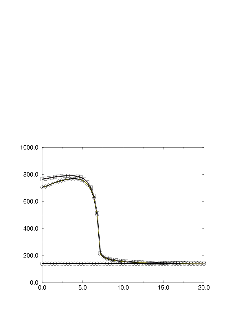
Figure 2: Spectrum of $\pi^{+}$: The first three singlet-s states in MeV versus $\mu/\kappa$.

Here comes the next problem: How should I determine the quark mass? In Eq.(11), I selected a particular value of $m$; I could have taken any other and would have gotten $\mu(m)$ and $\alpha_{\mu}(m)$. I obviously need a second empirical datum. Which one? I could choose the first excited state of $\pi^{+}$; but that is not known with sufficient accuracy for my purposes and, moreover, there are uncertainties of interpretation, see Morningstar [17] and Llanes-Estrada [18]. I could take the mass of the $\rho^{+}$; but the present $\uparrow\downarrow$-model is not particularly suited for vector mesons. I remain thus with the pions size. Knowing the wavefunction, see below, I could calculate the form factor [2] and thus the exact root-mean-square radius. But I replace this non-trivial calculation by the the following very drastic but simpler construction: I parametrize the numerical results by a fit function with one free parameter ($p_{a}$) to be,

$$\Phi_{a}(p)=\frac{10}{\left(1+\displaystyle\frac{p^{2}}{p_{a}^{2}}\right)^{2}},\hskip 30.00005pt\mathrm{with}\quad p_{a}=1.471\ \kappa.$$ (13)

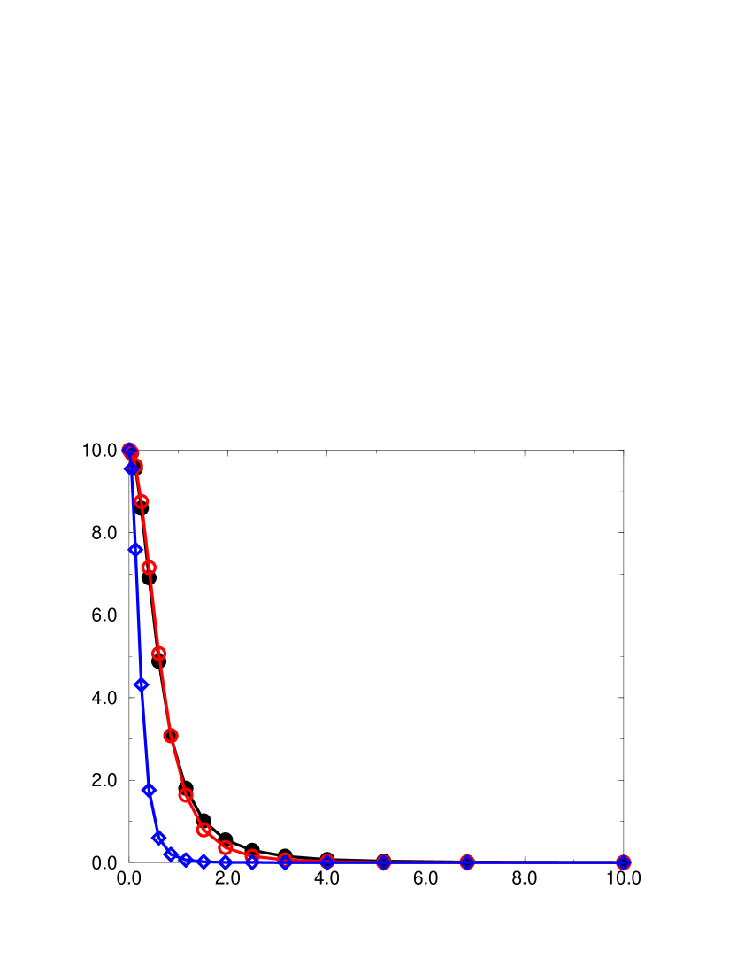
Figure 3: The pion wave function $\Phi(p)$ is plotted versus $p/(1.552\kappa)$ in an arbitrary normalization. The filled circles indicate the numerical results, the open circles the fit function. The diamonds denote the pure Coulomb solution.

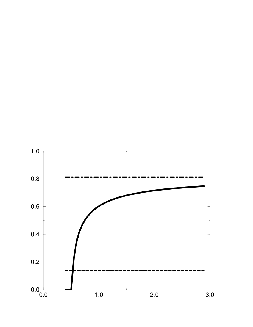
Figure 4: The relativistic potential energy $W(r)$ for the pion is plotted in GeV versus the radius in fm (solid line). The pion mass is indicated by the dashed, and the ionization threshold by the dashed-dotted line. See Eq.(16).

The quality of this fit can be judged by Fig. 4. I Fourier-transform this function to configuration space, giving $\psi(\vec{r})\sim e^{-p_{a}r}$, and calculate trivially

$$<r^{2}>^{\frac{1}{2}}_{\phi}=\frac{\sqrt{3}}{p_{a}}=0.663\mathrm{fm}.$$ (14)

Finally, I vary $m$ until I get about agreement with $<r^{2}>^{\frac{1}{2}}=0.657$ fm, the experimental value [15]. This exhausts all freedom in choosing the parameters of Eq.(8). Of course, the drastic assumption behind Eq.(14) has to replaced in the future by the correct prescription [20]. Actually, I had started the procedure with $m=1.00\ \kappa$. Eq.(11) quotes the result after iteration. After inserting the inverse Sawicki transformation Eq.(9) into the fit Eq.(13), I obtain

$$\psi(x,\vec{k}_{\!\perp})=\frac{1}{\sqrt{x(1-x)}}\frac{\mathcal{N}}{\left(1+\displaystyle\frac{m^{2}\left(2x-1\right)^{2}+\vec{k}_{\!\perp}^{\,2}}{4x(1-x)\ p_{a}^{2}}\right)^{2}}.$$ (15)

This completes my goal: I have a pion with the correct mass and size, and I have an analytic expression for its light-cone wave function.

For the first time in my life I see in Eq.(15) a genuine light-cone wave function, which is directly related to the QCD-Lagrangian (although only after quite a few approximations and simplifications). It could be used thus as a baseline for calculating the higher Fock-space amplitudes, as explained in [8]. It differs from the literature [19] by the preceding factor. I like to emphasize that regulated delta-interaction, the Yukawa potential in Eq.(8) at the scale $\mu_{0}$, acts like a genuine Dirac-delta function: it pulls down essentially only one state, the pion, in analogy with the pairing model [13]. The others are left more or less unperturbed at their Bohr values, see Fig. 2. I like to emphasize further that I am not in conflict with the usual perturbative inclusion of the hyperfine interaction. For sufficiently large values of $\mu$, say for $\mu\gg 10$, see Fig. 2, the coupling constant decreases strongly and the spectrum becomes more and more the familiar Bohr spectrum with a small hyperfine shift, such that it can be calculated perturbatively, indeed. In a future and more rigorous solution of the full equation I expect that the excited states can be disentangled into almost degenerate singlets and triplets, which in turn can be interpreted as an excitation of the pseudo-scalar pion, or the ground state of a vector meson, respectively. In any case, the first excited state of the simple model correlates very well with the mass of the $\rho^{+}$ and the other vector mesons, see below.

3 Extensions and conclusions

I can apply the same procedure also to the other mesons. Once I have the up and down mass, I determine the strange, charm and bottom quark mass by reproducing the masses of the $K,^{-}$ $D^{0}$ and $B,^{-}$ respectively. This gives $m_{s}=508$, $m_{c}=1666$ and $m_{b}=5054\mbox{ MeV}$. All these numbers as well as those in Tables 2 and 2 are rounded for convenience; the calculations or the experiments are available with greater precision. This fixes all parameters which there possibly are. I generate with them all off-diagonal pseudo-scalar mesons and compile their mass in Table 2. The corresponding wave functions are also available but not shown. In view of the simplicity of the model, the agreement with the empirical values in Table 2 is remarkable. The mass of the first excited states in Table 2 correlates astoundingly well with the associated vector meson in Table 2.

Table 1: The calculated mass eigenvalues in MeV. Those for singlet-1s states are given in the lower, those for singlet-2s states in the upper triangle.

	$\overline{u}$	$\overline{d}$	$\overline{s}$	$\overline{c}$	$\overline{b}$
$u$		768	871	2030	5418
$d$	140		871	2030	5418
$s$	494	494		2124	5510
$c$	1865	1865	1929		6580
$b$	5279	5279	5338	6114

Table 2: The empirical masses of the flavor-off-diagonal physical mesons in MeV. The vector mesons are given in the upper, the scalar mesons in the lower triangle.

	$\overline{u}$	$\overline{d}$	$\overline{s}$	$\overline{c}$	$\overline{b}$
$u$		768	892	2007	5325
$d$	140		896	2010	5325
$s$	494	498		2110	—
$c$	1865	1869	1969		—
$b$	5278	5279	5375	—

After so many years, I am forced to conclude that the pion looks quite a bit different than told in the literature. Although the above picture is kind of wood-carved, the previous work with Kalloniatis and Pinsky lets appear it unlikely that the zero modes, once included, change the picture drastically. I have found no evidence that the vacuum condensates are important. I conclude that the pion is describable by a QCD: The very large coupling constant in conjunction with a very strong hyperfine (spin-spin-) interaction makes it a ultra strongly bounded system of constituent quarks. More then 80% of the constituent quark mass is eaten up by binding effects. No other physical system has such a property. But this pion is not the one I was dreaming of when this work began.

The theory has three parameters. Two are determined by the pions mass and size, and one determines itself from the theory. In the lack of further empirical data, I have no independent check for the above strong statements, except that the first excited state should roughly be degenerate with the mass of the $\rho$-meson. At present I am working on a check [20] whether Eq.(15) is consistent with Ashery’s experiment [21].

The question of confinement is closely related to a the potential, the strong potential $V_{s}(r)$, but in the present approach the relation is subtle. One of the great advantages of light-cone quantization is the additivity of the free part and the interaction. Because of the dimensions of invariant mass squares the relation of potential and kinetic energy is somewhat hidden. What I can do, however is to Fourier transform Eq.(8) and to interpret the operators $\vec{p}$ and $\vec{q}$ as the classical analogue of momentum and position. Instead of an Hamiltonian $H(q,p)$ I then have an invariant mass-squared $M^{2}(q,p)$, but for the argument that does not matter. I thus have

$$M(r,p) = m_{s}\sqrt{1+\frac{p^{\,2}}{m_{s}m_{r}}+\frac{2}{m_{s}}V_{s}(r)},\hskip 3.00003ptV_{s}(r)\equiv\frac{4\alpha}{3r}\left(1+\frac{\mu^{2}}{m_{s}m_{r}}\mathrm{e}^{-p_{a}r}\right).$$ (16)

The expansion into rest mass + kinetic energy + potential energy,

$$M(r,p)\simeq m_{s}+\frac{p^{\,2}}{2m_{r}}+V_{s}(r),$$ (17)

is justified however only for $p^{\,2}\ll{m_{s}m_{r}}$, and $V_{s}(r)\ll{m_{s}}$, which can not be satisfied for all $r$. I therefore propose to introduce a relativistic potential energy by $W(r)\equiv M(r,p=0)$ as the closest relativistic analogue to a non-relativistic potential $V_{s}(r)$, which we all have in the back of our mind. This function is plotted in Fig. 4. It vanishes at $r_{0}=0.5194$ fm and the classical turning point is $r_{t}=0.5300$ fm. Since the sum of the quark masses is 812 MeV, the ionization threshold occurs at 542 MeV: In order to liberate the quarks in the pion, one has to invest more than three times the rest mass of a pion; I call this practical confinement.

I contrast these results to Lattice Gauge Calculations. It is not generally known that LGC’s have considerable uncertainty to extrapolate their results down to such light mesons as a pion; it exceeds their grid sizes. It is also not generally known that Lattice Gauge Calculations get always strict and linear confinement even for QED, where we positively know the ionization threshold. The ‘breaking of the string’, or in a more physical language, the ionization threshold is one of the hot topics at the lattice conferences [22]. Moreover, in order to get the size of the pion, thus the form factor, requires another generation of computers and physicists to run them.

I contrast these results also to phenomenological approaches. They usually do not address to get the pion, and for the heavy mesons, where they are so successful, a good phenomenological model has quite many parameters, in any case more that the above canonical ones. A detailed comparison and systematic discussion of the bulky literature can however be postponed, until we are ready to solve the full Eq.(1) and do not restrict ourselves to the caricature of the QCD-interaction, the $\uparrow\downarrow$-model.

I contrast these results, finally, to the Nambu-Jona-Lasio-based models which are so successful in accounting for the isospin. I do not even think of quoting from the huge body of literature but mention in passing that the NJL-models are not renormalizable, have no relation to QCD, and deal mostly with the very light mesons. They just about can handle strangeness and break down for the heavy flavors.

In conclusion I may state that not a single model can describe quantitatively all mesons from the $\pi$ up to the $\Upsilon$ from a common point of view, from QCD. By solving the $\uparrow\downarrow$-model I provide at least some evidence that Eq.(1) can eventually give that, perhaps sometimes in the future.

Acknowledgement. I thank Susanne Bielefeld for her unselfish help during the past three years.

References

- [1] P.A.M. Dirac, Rev. Mod. Phys. 21 (1949) 392.
- [2] S.J. Brodsky, H.C. Pauli, and S.S. Pinsky, Phys. Rep. 301 (1998) 299-486.
- [3] Compendium, in the appendix to this volume.
-
[4]
A.C. Kalloniatis and H.C.Pauli,
Z. Phys. C60 (1993) 255;
A.C. Kalloniatis, H.C. Pauli, and S.S. Pinsky, Phys. Rev. D50 (1994) 6633;
A.C. Kalloniatis, Phys. Rev. D54 (1996) 2876-2888. - [5] J. Hiller, this volume.
- [6] A.C. Tang, S.J. Brodsky, and H.C. Pauli, Phys. Rev. D44 (1991) 1842.
- [7] H.C. Pauli, Eur. Phys. J. C7 (1998) 289. hep-th/9809005.
- [8] H.C. Pauli, in: New directions in Quantum Chromodynamics, C.R. Ji and D.P. Min, Eds., American Institute of Physics, 1999, p. 80-139. hep-ph/9910203.
- [9] H.C. Pauli, this volume.
- [10] F. Wegner, this volume.
- [11] M. Krautgärtner, H.C. Pauli, F. Wölz, Phys. Rev. D45 (1992) 3755.
- [12] U. Trittmann and H.C. Pauli, this volume.
- [13] M. Brack, J. Damgaard, A.S. Jensen, H.C. Pauli, V.M. Strutinsky, and C.Y. Wong, Rev. Mod. Phys. 44 (1972) 302.
- [14] S. Bielefeld, J. Ihmels, and H.C. Pauli, hep-ph/9904241.
- [15] C. Caso et al., Eur.Phys.J. C3 (1998) 1.
- [16] H.C. Pauli, in: Adelaide proceedings.
- [17] C. Morningstar, this volume.
- [18] F. Llanes-Estrada, this volume.
- [19] G.P. Lepage and S.J. Brodsky, Phys. Rev. D22, 2157 (1980).
- [20] Collaboration with A. Mukherjee, initiated at this meeting.
- [21] D. Ashery, this volume.
- [22] K. Schilling, Nucl. Phys. Proc. Suppl. 83 (2000) 140.