PACS:13.60.Hb;14.80.-j;14.80.Ly
Estimates of threshold cross section for stoponium production at $e^{+}e^{-}$ colliders

We estimate the total $e^{+}e^{-}\to\tilde{t}\overline{\tilde{t}}$ cross section near threshold for a Coulombic potential and compare it to the Born approximation. The effect of the beam energy spread for present and future $e^{+}e^{-}$ colliders is discussed.

1 Introduction

In the Standard Model it has been shown that bound states can be created for every quark but the top (see for instance [1, 2, 3, 4, 5] and references therein). The latter possibility is ruled out due to the high value of the top quark mass, which is responsible for its short lifetime. The top quark decays directly into a $W$ boson and a $b$ quark before being able to create a bound state. In a recent paper [6] it has been shown that a finite probability of formation exists for a supersymmetric bound state made out of a squark stop and an antitop squark, for a certain range of $\tilde{t}$ mass and some regions of the MSSM parameter space. In that, the possibility of signal detection at an $e^{+}e^{-}$ collider with LEP and NLC characteristics has also been investigated by means of a Breit–Wigner formula.

A more refined result is needed in the threshold region which is characterised by low values of the squark velocity $\beta$, i.e.

$$\beta=\sqrt{1-\frac{4m_{\tilde{t}}^{2}}{s}}\ll 1\qquad.$$ (1)

For this purpose a by now standard Green function approach has been developed (see [1], [7], [8] and references therein).

We will assume that the supersymmetric bound state creation does not differ from the standard model case, as the relevant interaction is driven by QCD and controlled by the mass of the constituent squarks [6]. For this reason the Schrödinger Green function technique is suitable for treating the problem of the scalar bound state. It will be used to compute the bound state effects on the cross section of stoponium near threshold. We will compare the results obtained in this manner to the Born cross section estimates for energies above threshold. The effects of the beam energy spread of the $e^{+}e^{-}$ colliders on the computed cross section will be discussed.

2 The method

The basic idea of the method is to consider the Schrödinger Green function equation [1]

$$(\mathbf{H}-E)G(\mathbf{x},\mathbf{y},E)=\delta(\mathbf{x}-\mathbf{y})\qquad,$$ (2)

where $\mathbf{H}$ is the Hamiltonian of the system

$$\mathbf{H}=-\frac{\nabla_{\mathbf{x}}^{2}}{2m}+V(\mathbf{x})\qquad,$$ (3)

and $V(\mathbf{x})$ is the potential for the squarks. The imaginary part of the derivative of the Green function given by (2) taken at the origin is proportional to the cross section at threshold [1, 7, 8]. The finite width $\Gamma$ of the state is taken into account by the substitution

$$E\to E+i\Gamma\qquad.$$ (4)

Unlike the process

$$e^{+}e^{-}\to t\bar{t}\qquad,$$ (5)

the reaction

$$e^{+}e^{-}\to\tilde{t}\overline{\tilde{t}}$$ (6)

proceeds in P–wave, whereas top quarks are produced in S–wave configuration. This implies the Born level cross section to grow as $\sigma\sim\beta$ for top production (5), while for process (6) of scalars one obtains a slower rise, $\sigma\sim\beta^{3}$.

The threshold cross section of the process $e^{+}e^{-}\to\tilde{t}\overline{\tilde{t}}$ is given by the following expression [9, 10]:

$$\sigma(e^{+}e^{-}\to\tilde{t}\overline{\tilde{t}})=R\;\frac{\pi\alpha^{2}}{s} \times \left[\tilde{Q}_{\gamma}^{2}+\frac{(v_{e}^{2}+a_{e}^{2})\tilde{Q}_{Z}^{2}}{4\sin^{2}2\theta_{W}}\frac{s^{2}}{(s-M_{Z}^{2})^{2}+M_{Z}^{2}\Gamma_{Z}^{2}}+\right.$$ (7)

$$\hphantom{\frac{\pi\alpha^{2}\beta^{3}}{s}a}\left.+\,\frac{v_{e}\tilde{Q}_{\gamma}\tilde{Q}_{Z}}{\sin 2\theta_{W}}\frac{s(s-M_{Z}^{2})}{(s-M_{Z}^{2})^{2}+M_{Z}^{2}\Gamma_{Z}^{2}}\right]$$

where $v_{e}=-1+4\sin^{2}\theta_{W}$, $a_{e}=-1$, $M_{Z}$ and $\Gamma_{Z}$ are the mass and the total width of the $Z$ boson respectively. The charges are defined by $\tilde{Q}_{\gamma}=-Q$, $\tilde{Q}_{Z}=(\cos^{2}\theta_{\tilde{t}}-2Q\sin^{2}\theta_{W})\sin 2\theta_{W}$ , with $\theta_{W}$ being the standard electroweak mixing angle and $\theta_{\tilde{t}}$ is the left–right mixing angle.

The $R$ term of equation (7) is obtained [1, 7, 8] upon taking the imaginary part of the derivative at the origin of the Green function given by (2)

$$R=\frac{1536}{81}\frac{\pi}{m_{\tilde{t}}^{4}}\Im\left[\left.\frac{\partial}{\partial\mathbf{x}}\frac{\partial}{\partial\mathbf{y}}G_{1}(\mathbf{x},\mathbf{y},E)\right]\right|_{\mathbf{x}=0,\mathbf{y}=0}$$ (8)

($\Im$ stands for the imaginary part, while $G_{1}$ is the $l=1$ component of the Green function).

For the purpose of our investigation, we will use a Coulombic potential for the Hamiltonian given in (3) (here $r=|\mathbf{x}|)$

$$V=-\frac{4}{3}\frac{\alpha_{s}}{r}$$ (9)

where $\alpha_{s}$ is given by the QCD two–loop expression [11]

$$\alpha_{s}(Q^{2})=\frac{4\pi}{\beta_{0}\log\left[Q^{2}/\Lambda^{2}_{\overline{MS}}\right]}\left\{1-\frac{2\beta_{1}}{\beta_{0}^{2}}\frac{\log\left[\log\left[Q^{2}/\Lambda^{2}_{\overline{MS}}\right]\right]}{\log\left[Q^{2}/\Lambda^{2}_{\overline{MS}}\right]}\right\}$$ (10)

and is calculated at a fixed value of the Bohr radius $r_{B}$ given by

$$r_{B}=\frac{3}{2m_{\tilde{t}}\alpha_{s}}\qquad.$$ (11)

The validity of this choice has been shown (see  [5, 6, 12] and references therein), and is essentially justified by the fact that the stop quark should be much heavier than all other quarks except (maybe) the top. The high value of $m_{\tilde{t}}$ implies from (11) that the average distance between two squarks inside the scalar bound state is small, and therefore the dominant term of the potential is the Coulomb expression given in (9). This assumption for the bound state potential allows us to obtain an analytic expression for the Green function needed for the threshold cross section [13].

Following the above cited authors we introduce some standard notations: $E=\sqrt{s}-2m_{\tilde{t}}$ is the energy displacement from threshold, $k^{2}=-m_{\tilde{t}}E$, $\lambda=3\alpha_{s}m_{\tilde{t}}/2$ is the wavelength, and $\nu=\lambda/k$ is the wave number. Here the argument of $\alpha_{s}$ is taken to be at the soft scale $1/r_{B}$ . The finite width $\Gamma$ of the bound state is taken into account by means of the substitution given in (4).

The expression for the $l=1$ Green function for the Coulombic potential (9) is given by

$$G_{1}(0,0,k)=\qquad\qquad\qquad\qquad\qquad$$

$$=\frac{m_{\tilde{t}}}{36\pi}\lambda\left\{2(k^{2}-\lambda^{2})\left[\frac{k}{2\lambda}+\ln\left(\frac{k}{\mu_{f}}\right)+2\gamma_{E}-\frac{11}{6}+\psi_{1}(1-\nu)\right]+\frac{k^{2}}{2}\right\}$$ (12)

where $\gamma_{E}$ is Euler constant ($\simeq 0.57721$), and $\psi_{1}$ is the digamma function, $\psi_{1}(x)=d(\ln\Gamma(x))/dx$. The derivative at the origin of (12) is obtained by the simple multiplicative relation

$$\left.\frac{\partial}{\partial\mathbf{x}}\frac{\partial}{\partial\mathbf{y}}G_{1}(\mathbf{x},\mathbf{y},k)\right|_{\mathbf{x}=0,\mathbf{y}=0}=9G_{1}(0,0,k)\qquad.$$ (13)

Some caveats (as described in [13]) have to be considered for the case of the $P$ wave. There exists a constant linear term in the decay width $\Gamma$ contributing to the $l=1$ Green function that cannot be properly computed in a purely nonrelativistic framework [7]. The term independent from $k$ that has to be added to the Green function (12) is given by

$$0.185\frac{m_{\tilde{t}}^{3}}{36\pi}\Gamma$$ (14)

and from [13] the $\mu_{f}$ argument of the logarithmic term in (12) is given by $0.13m_{\tilde{t}}$ by means of an analysis of relativistic perturbation theory. We note that the last two results have been obtained only for the top quark case, and we will assume that those results remain valid also for the stop quark which has a high mass, presumably close to that of the top quark. In any case the two aforementioned terms do not contribute much to the Green function estimates, since they are dominated by the leading $k^{3}$ term of (12).

3 Results and discussion

Our analysis of the threshold behaviour of the cross section should hold for a range of mass values and decay widths. For the mass range we will refer to the current stop mass value limits [14] and the LEP capabilities, while for the decay widths we have to take into account the formation requirements of the bound state [6]. A criterion for the formation of bound states is that the creation of a hadron can occur only if the level splitting which depends upon the strength of the strong force between the (s)quarks and their relative distance [4], is larger than the natural width of the state. This means that, if

$$\Delta E_{2P-1P}\geq\Gamma$$ (15)

where $\Delta E_{2P-1P}=E_{2P}-E_{1P}$ and $\Gamma$ is the width of the would–be bound state, then the bound state exists. Performing the analysis in this way allows us also to avoid dealing directly with several parameters of the MSSM model which are relevant to stop quark decay (apart from the stop mass), namely the ratio of the two Higgs vacuum expectation values $\tan\beta$, the Higgs–higgsino mass parameter $\mu$ and the wino mass $M_{2}$ [10]. The only constraint we have to impose is that the decay width be lower than about 1 GeV, necessary for the scalar bound state creation [6] regardless of the values assumed for the parameters mentioned above.

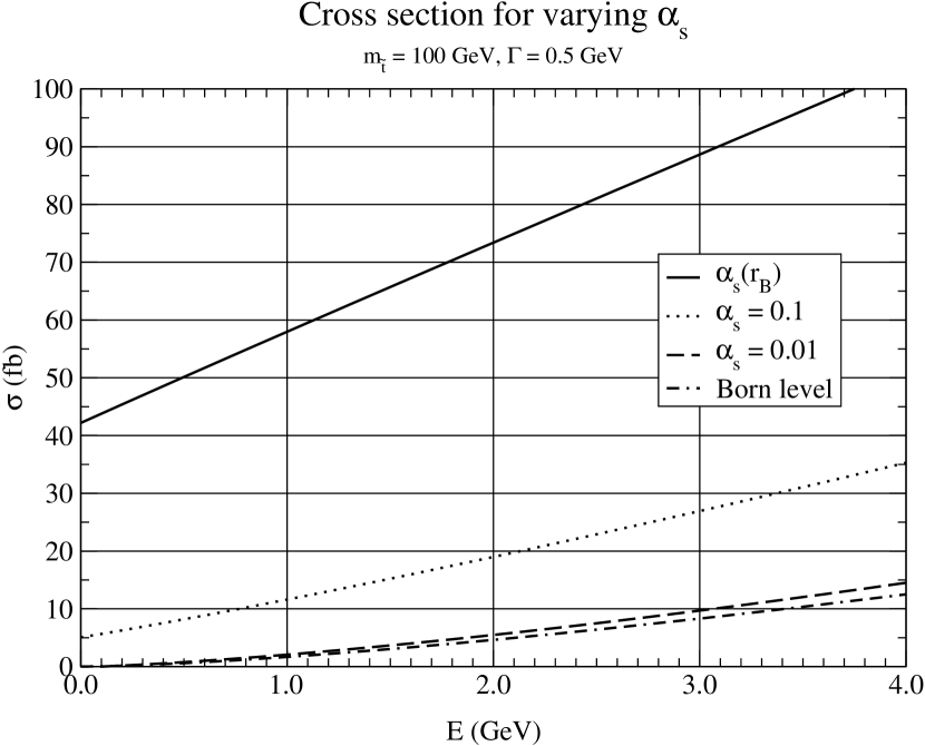
Figure 1: Comparison of the Green function method and the Born level expression for the cross section, in the limit $\alpha_{s}\to 0$. Here we assume that $\cos^{2}\theta_{\tilde{t}}=1$, $m_{\tilde{t}}=100\;GeV$ and a width of 0.5 GeV.

As a first step, we check that the expression (12) used for our potential model (9) is consistent with the Born cross section for $E>0$. We see in figure (1) that in the non interacting limit with $\alpha_{s}\to 0$ the cross section given by (12) tends to the usual Born expression, and is zero for $E<0$. This confirms the consistency of the expression found in (7).

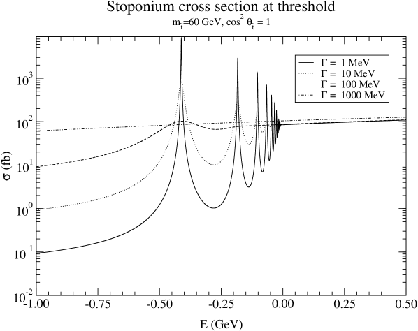
Figure 2: Cross section at threshold for various decay widths with $m_{\tilde{t}}=60\;GeV$, $\cos^{2}\theta_{\tilde{t}}=1$. The centre of mass energy is $\sqrt{s}=120\;GeV$ at threshold.

In figures (2,3) we present the results of the threshold cross section for a LEP mass range, $m_{\tilde{t}}=60,\>100\>GeV$. We have chosen the left–right mixing angle to be such that $\cos^{2}\theta_{\tilde{t}}=1$. From (7) it is possible to see that the cross section minimum value is obtained for $m_{\tilde{t}}=100\>GeV$ at $\cos\theta_{\tilde{t}}\simeq\pm 0.55$, the point where the $Z$ boson coupling vanishes, which does not much differ from the maximal value. As previously stated, assuming the decay width to be smaller than 1 $GeV$, we show for each chosen mass for widths of $10^{-3},10^{-2},10^{-1}$ and 1 $GeV$ respectively. The cross sections are plotted against the threshold offset energy $E$, the centre of mass energy being given by the relation $\sqrt{s}=2m_{\tilde{t}}+E$.

For $m_{\tilde{t}}=60\;GeV$, figure (2) shows the structure of the discrete energy levels for $E<0$ versus decay width values given above. The maximal height of the peak, about 8400 $fb$, is obtained for the smallest width of $1\;MeV$. The shape of the peaks are similar to the one obtained by the Breit–Wigner formula, except for the resonance tails that are set higher with increasing energy. The height of the peaks decreases drastically as the binding energy reaches asymptotically the $E=0$ level. They tend also to accumulate and merge towards the $E=0$ value as the energy increases; this happens when the distance of the two resonance peaks is of the order of the decay width. For the Coulombic model the binding energy of the $l=1$ level is given by the expression

$$E_{n}=-\frac{4}{9}\frac{m_{\tilde{t}}\alpha_{s}^{2}}{n^{2}}\quad,\;n>1$$ (16)

and the resonance peaks merge when

$$\frac{4}{9}m_{\tilde{t}}\alpha_{s}^{2}\left[\frac{1}{n^{2}}-\frac{1}{(n+1)^{2}}\right]\sim\Gamma\qquad.$$ (17)

This means that the the last visible peak has a quantum number $n$ given by

$$\frac{2n+1}{n^{2}(n^{2}+1)}\sim\frac{9\Gamma}{4m_{\tilde{t}}\alpha_{s}^{2}}\qquad,$$ (18)

we can see for instance in plot (2) that for $\Gamma=0.1\;GeV$ the $n=3$ peak is already barely noticeable. For $\Gamma=1\;GeV$, the limiting region of bound state formation [6], we see that there is no visible structure; even the first peak is smeared by the large width.

The continuum energy region $E>0$ does not present any fine structure, and remains essentially the same for any given decay width. One important effect to be noted is the large difference of the Green function result with respect to the Born prediction for $E>0$. This fact is shown in figure (1) where the two estimates of the cross section are compared. It is clearly seen that the former is about one order of magnitude larger than the Born cross section. This can be understood by the fact that the Green function technique takes into account the interaction between the particles, and the contributions of the binding energies accumulate towards the $E=0$ energy level as described, thus affecting substantially the continuum region as well.

In figure (3), we show the results for $m_{\tilde{t}}=100\;GeV$, with the same parameters given in figure (2). The peaks are lower than the previous case, in particular the largest value of the cross section is obtained for $\Gamma=1\;MeV$ at about 2400 $fb$. The position of the peaks are shifted towards lower values of the centre of mass energy because the binding energy given by the expression (16) is higher.

For NLC energies, we present in figures (4) and (5) results obtained for $m_{\tilde{t}}=200\;GeV$ and $m_{\tilde{t}}=500\;GeV$ respectively. The parameters have been chosen to be the same as of the LEP case, and the qualitative behaviour of the threshold cross section is analogous. For $m_{\tilde{t}}=200\;GeV$, the maximal value of the first peak obtained at $\Gamma=1\;MeV$ is about 450 $fb$, while for $m_{\tilde{t}}=500\;GeV$ the highest peak reaches only 90 $fb$. The position of the peaks is shifted towards even lower energy values because of still higher values of bound state binding energy, as can be verified from (16).

We remark that all our results have been obtained for the Coulombic potential (9). It is known that in the threshold region there are singular Coulombic terms $(\alpha_{s}/\beta)^{n}$ which spoil the finite order perturbation theory. The resummation of these contributions have been done – see [13] and references therein – and they give small contributions and only modify slightly the Coulombic potential. The effect on the cross section is quite small, as can be seen from the plots in [13], and does not change our estimates by more than a few percent.

Another point concerns the validity of the Schrödinger Green function method (12). Since it is a nonrelativistic procedure, we have to ensure that the velocity of the squarks is low enough in order to make relativistic corrections negligible. From kinematical arguments, it is possible to give a bound for the maximal acceptable energy offset $E_{MAX}$ . Assuming an upper value for the squark velocity, $\beta_{MAX}$ , and the expression (1) together with the centre of mass energy parametrisation, $\sqrt{s}=2m_{\tilde{t}}+E$, one obtains by means of a series expansion in $E$

$$E_{MAX}<m_{\tilde{t}}\beta_{MAX}^{2}\qquad.$$ (19)

In table (1) we present some estimates on $\beta_{MAX}$ and $E_{MAX}$ for different squark masses and some Lorentz $\gamma$ parameter values. We see that the limit of validity for the nonrelativistic equation (2) lies in a range of a few $GeV$ around the threshold, and naturally increases with larger squark masses; this can be intuitively understood since the heavier the squark is, the slower will it rotate inside the bound state [2, 4, 5, 6].

The results obtained so far have to be folded with the beam energy spread of the collider. For the LEP2 case, which has a beam energy spread of the order of 200 $MeV$ [14], even if the peak cross section is in the $nb$ range for $m_{\tilde{t}}=60\;GeV$ (2) the various resonance peaks are practically undetectable because their widths are much smaller than the typical beam energy spread (see also the discussion of [6]). The sole possibility of a width larger than the beam energy spread, $\Gamma=1\;GeV$ case, as already discussed, has no peaks as they have been smeared and thus no visible fine structure is envisaged. The situation does not change for the value of $m_{\tilde{t}}=100\;GeV$; as we can see from figure (3) this situation is essentially the same as the previous one, and the peak cross section is even smaller than the former by a multiplicative factor of about 4.

With the increase of the centre of mass energy (NLC case) the net result for the cross section detection is even worse than before. The beam energy spread is of the order of 6 $GeV$ [15] and, as seen clearly from figures (4) and (5), it is even larger than the energy range used for the plots by a factor of 4, thus making impossible the detection of any possible fine structure present in the threshold cross section.

4 Conclusions

In this letter, we have shown that the bound state effect on the threshold cross section of a scalar stop bound state is not negligible, at least for the case of a Coulombic potential. This effect turns out to be also dramatically different from the simple Born cross section results for $E>0$ [10, 16].

However, because of the large beam energy spread of the present (LEP2) and future (NLC) $e^{+}e^{-}$ colliders, the possible structure of the cross section at threshold cannot be resolved. This confirmes our less refined Breit–Wigner approach of [6], and reinforces our previous result that the stoponium cannot be detected at the present and even future $e^{+}e^{-}$ colliders.

Acknowledgements

The author wishes to thank M. Antonelli for useful discussion and support during this work; and also O. Panella and P. Gensini for helpful hints. Many thanks also to Y. Srivastava for careful reading and patiently correcting the manuscript.

Limits of nonrelativistic approach

$\gamma$	$\beta_{MAX}$	$E_{MAX}(60)$	$E_{MAX}(100)$	$E_{MAX}(200)$	$E_{MAX}(500)$
1.01	0.140	1.18	1.97	3.94	9.85
1.02	0.197	2.33	3.88	7.77	19.42
1.03	0.240	3.44	5.74	11.48	28.70

Table 1: Some estimates on $\beta_{MAX}$ and $E_{MAX}$ as a function of the $\gamma$ parameter for various stop masses, indicated in brackets, in $GeV$ units.

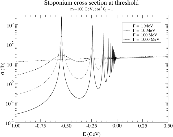
Figure 3: Cross section at threshold for various decay widths with $m_{\tilde{t}}=100\;GeV$, $\cos^{2}\theta_{\tilde{t}}=1$. The centre of mass energy is $\sqrt{s}=200\;GeV$ at threshold.

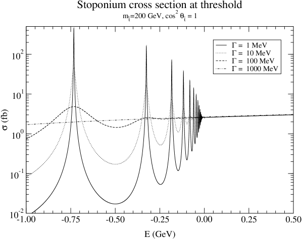
Figure 4: Cross section at threshold for various decay widths with $m_{\tilde{t}}=200\;GeV$, $\cos^{2}\theta_{\tilde{t}}=1$. The centre of mass energy is $\sqrt{s}=400\;GeV$ at threshold.

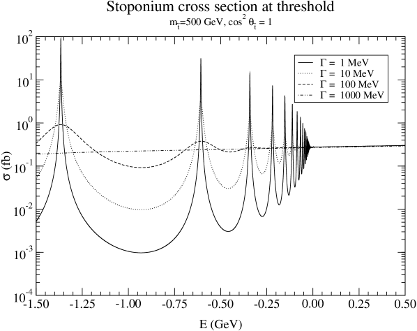
Figure 5: Cross section at threshold for various decay widths with $m_{\tilde{t}}=500\;GeV$, $\cos^{2}\theta_{\tilde{t}}=1$. The centre of mass energy is $\sqrt{s}=1000\;GeV$ at threshold.

References

-
[1]
V.S. Fadin, V.A. Khoze, JETP Lett 46 525 (1987);
V.S. Fadin, V.A. Khoze, Yad. Fiz. 48 487 (1988);
- [2] G. Pancheri, J.P. Revol and C. Rubbia, Phys. Lett. B 277 518 (1992).
-
[3]
J.H. Kühn, E. Mirkes, Phys. Lett. B 296 425 (1992);
J.H. Kühn, E. Mirkes, Phys. Rev. D 48 179 (1993). - [4] N. Fabiano, Eur. Phys. J. C 2 345 (1998).
-
[5]
N. Fabiano, A. Grau and G. Pancheri, Phys. Rev. D 50 3173 (1994);
Nuovo Cimento A, Vol. 107, 2789, (1994). - [6] M. Antonelli, N. Fabiano, Eur. Phys. J. C16 361 (2000).
-
[7]
V.S. Fadin, V.A. Khoze, Yad. Fiz. 93 1118 (1991);
I.I. Bigi, V.S. Fadin and V.A. Khoze, Nucl. Phys. B 377 461 (1992);
I.I. Bigi, F. Gabbiani and V.A. Khoze, Nucl. Phys. B 406 3 (1993);
J.H. Kühn, E. Mirkes and J. Steegborn, Z. Phys. C 57 615 (1993);
W. Mödritsch, Nucl. Phys. B 475 507 (1996). -
[8]
W. Kwong, Phys. Rev. D 43 1488 (1991);
M.J. Strassler, M.E. Peskin, Phys. Rev. D 43 1500 (1991);
M. Jezabek, J.H. Kühn and T. Teubner, Z. Phys. C 56 653 (1992);
Y. Sumino et al., Phys. Rev. D 47 56 (1993). - [9] W. Beenakker, R. Hopker and P.M. Zerwas, Phys. Lett. B 349 463 (1995).
- [10] K. Hikasa, M. Kobayashi, Phys. Rev. D 36 724 (1987).
-
[11]
W.A. Bardeen, A.J. Buras, D.W. Duke and T. Muta, Phys. Rev.
D 18 3998 (1978);
W.J. Marciano, Phys. Rev. D 29 580 (1984). - [12] N. Fabiano, Eur. Phys. J. C 2 345 (1998).
-
[13]
A.A. Penin, A.A. Pivovarov, Nucl. Phys. B 550 375 (1999);
hep-ph/9904278. -
[14]
Review of Particle Properties, EuroPhys. Journ. C 3 1 (1998);
http://pdg.lbl.gov/ -
[15]
Ed. R. Brinkmann, G. Materlik, J. Rossbach, A. Wagner,
Conceptual Design of a 500 GeV Linear Collider with Integrated
X–Ray Laser Facility, Vol. 1 (1997);
Ron Settles, private communication;
Marcello Piccolo, private communication. - [16] M. Drees, K. Hikasa, Phys. Lett. B 252 127 (1990).