Ground and excited scalar isoscalar meson states in a $U(3)\times U(3)$ quark model with a glueball.

Abstract

Ground and first radially excited scalar isoscalar meson states and a scalar glueball are described in a nonlocal $U(3)\times U(3)$ quark model. The glueball is introduced into the effective meson Lagrangian by means of the dilaton model on the base of the scale invariance of the meson Lagrangian. The scale invariance breaking by current quark masses and gluon anomalies is taken into account. The glueball anomalies turn out to be important for the description of the glueball-quarkonia mixing. The masses of five scalar isoscalar meson states and their strong decay widths are calculated. The state $f_{0}(1500)$ is shown to be composed mostly of the scalar glueball.

1 Introduction

In our recent papers [1, 2, 3], it was shown that the experimentally observed scalar meson states lying in the mass interval from 0.4 to 1.7 GeV [4] can be interpreted as two nonets of scalar quarkonia: the ground state nonet (with masses below 1 GeV) and the nonet of their first radial excitations (heavier than 1 GeV). Meanwhile, it is established from experiment that another scalar isoscalar meson state exists in this mass interval [4]. It is used to be associated with the scalar glueball. The most probable candidates for the glueball are the states $f_{0}(1500)$ and $f_{0}(1710)$ [5, 6, 7]. In [1, 2, 3], we came to the conclusion that $f_{0}(1710)$ is rather a quarkonium, while $f_{0}(1500)$ is a glueball. This is in agreement with the results given in [5]. However, to make the final decision, one should introduce the glueball into the effective meson Lagrangian. Our present paper is devoted to solution of this problem.

A nonlocal version of the $U(3)\times U(3)$ chiral quark model with the local ’t Hooft interaction [1, 2, 3] was used to describe the meson nonets mentioned above. The nonlocality was introduced there by means of form factors in quark currents. This allowed us to describe the nonet of first radial excitations [3, 8, 9]. The form factors were chosen so that they allow to satisfy the low-energy theorems in the chiral limit and keep gap-equations in a form derived from the standard Nambu–Jona-Lasinio (NJL) model. In the momentum space, these form factors are expressed through first degree polynomials depending on the momentum squared and have a Lorentz-covariant form. The masses and decays of the ground and radially excited nonets of scalar, pseudoscalar, and vector mesons were described in the framework of this model [1, 2, 3]. However, we did not consider the glueball. Here we suggest an extended version of the non-local $U(3)\times U(3)$ quark model that gives a description of the scalar glueball as well as the ground and radially excited scalar quarkonia nonets.

A common method of introducing the glueball into the effective meson Lagrangian is to take advantage of the dilaton model. The dilaton model was used by many authors [6, 10, 11] for this purpose. These models are based on the approximate scale invariance of the effective meson Lagrangian, which is in accordance with the QCD Lagrangian scale invariance if the current quark masses are equal to zero. As in QCD, in the effective meson Lagrangian, the terms with current quark masses also break scale invariance. Moreover, the scale invariance is broken by terms induced by gluon anomalies, which is also in accordance with QCD. All the terms that break scale invariance turn out to be important for the description of the quarkonia-glueball mixing and, as a consequence, have a noticeable effect on the strong decay modes of scalar mesons.

In papers [12, 13, 14], we constructed a model describing only the ground scalar isoscalar meson states and a glueball. It was shown that the state $f_{0}(1500)$ is rather the scalar glueball than $f_{0}(1710)$. We described its decays in satisfactory agreement with available experimental data. We also found that the terms connected with gluon anomalies determine the most of quarkonia-glueball mixing.

Here, we extend our model to describe both the ground and radially excited scalar isoscalar quarkonia as well as the scalar glueball state. Thereby, we obtain the complete description of 19 scalar meson states within the mass interval from 0.4 to 1.7 GeV. Our approach and results noticeably differ from those given in [6, 15]. Moreover, for the first time, we succeeded to describe the nature of all 19 scalar meson states.

Insofar as we cannot expect that the chiral symmetry can determine the properties of so heavy particles well enough, we claim here only qualitative agreement of our results with experiment. Only isoscalar states are considered. Concerning the isovector and strange mesons, the introduction of the scalar glueball changes little the results obtained for them in [1, 2, 3].

The structure of our paper is following. In section 2, a nonlocal chiral quark model of the NJL type with the local six-quark ’t Hooft interaction is bosonized to construct an effective meson Lagrangian. In section 3, the meson Lagrangian is extended by introducing a scalar glueball as a dilaton on the base of scale invariance. The gap equations, the divergence of the dilatation current and quadratic terms of the effective meson Lagrangian are derived in sect. 4. There, we also diagonalize quadratic terms. Numerical estimates of the model parameters are given in sect. 5. In section 6, the widths for the main modes of strong decays of scalar isoscalar mesons are calculated. The discussion over the obtained results is given in sect. 7. A detailed description of how to calculate the quark loop contribution to the width of strong decays of scalar mesons is given Appendix A.

2 $U(3)\times U(3)$ Lagrangian for quarkonia

We start from an effective $U(3)\times U(3)$ quark Lagrangian of the following form (see [1, 2, 3]):

$$L = L_{\rm free}+L_{\rm NJL}+L_{\rm tH},$$ (1)

$$L_{\rm free} = {\bar{q}}(i{\hat{\partial}}-m^{0})q$$ (2)

$$L_{\rm NJL} = {G\over 2}\sum_{i=1}^{N}\sum_{a=1}^{9}[({j}_{{\rm S},i}^{a})^{2}+({j}_{{\rm P},i}^{a})^{2}]$$ (3)

$$L_{\rm tH} = -K\left\{{\det}[{\bar{q}}(1+\gamma_{5})q]+{\det}[{\bar{q}}(1-\gamma_{5})q]\right\},$$ (4)

where $L_{\rm free}$ is the free quark Lagrangian with $q$ and $\bar{q}$ being $u$, $d$, or $s$ quark fields; $m^{0}$ is a current quark mass matrix with diagonal elements: $m^{0}_{\rm u}$, $m^{0}_{d}$, $m^{0}_{\rm s}$ $(m^{0}_{\rm u}\approx m^{0}_{d})$. The term $L_{\rm NJL}$ contains nonlocal four-quark vertices of the Nambu–Jona-Lasinio (NJL) type which have the current-to-current form. The quark currents are defined in accordance with [1, 2, 3, 8, 9]:

$${j}_{{\rm S(P)},i}^{a}(x)=\int\!d^{4}x_{1}d^{4}x_{2}\bar{q}(x_{1}){F}_{{\rm S(P)},i}^{a}(x;x_{1},x_{2})q(x_{2}),$$ (5)

where the subscript S is for scalar and P for the pseudoscalar currents. The term $L_{\rm tH}$ is the six-quark ’t Hooft interaction which is supposed to be local, so no form factor is introduced in $L_{\rm tH}$.

Currents (5) are nonlocal due to the nonlocal quark vertex functions ${F}_{{\rm S(P)},i}^{a}$. This way of introducing nonlocality allows to consider radially excited meson states, which is impossible in the standard NJL model. In general, the number of radial excitations $N$ is infinite, but we restrict our-selves with $N=2$, leaving only the ground and first radially excited states, because extending this model by involving more heavier particles is not valid for this class of models.

Let us define the quark vertex functions in the momentum space.

$${F}_{{\rm S(P)},i}^{a}(x;x_{1},x_{2})=$$

$$\quad=\int\!\frac{d^{4}P}{(2\pi)^{4}}\frac{d^{4}k}{(2\pi)^{4}}\exp\frac{i}{2}\biggl{(}(P+k)(x-x_{1})$$

$$\quad+(P-k)(x-x_{2})\biggr{)}{F}_{{\rm S(P)},i}^{a}(k|P),$$ (6)

where $P$ is the total momentum of a meson and $k$ is the relative momentum of quarks inside the meson. As it was mentioned in the Introduction, here we follow papers [1, 2, 3, 8, 9], where the functions ${F}_{{\rm S(P)},i}^{a}(k|P)$ are chosen in the momentum space as follows:

$${F}_{{\rm S},i}^{a}(k|P)=\tau_{a}f_{i}^{a}(k_{\perp}),\quad{F}_{{\rm P},i}^{a}(k|P)=i\gamma_{5}\tau_{a}f_{i}^{a}(k_{\perp}),$$ (7)

and the form factors $f_{i}^{a}$, $(i=1,2)$ are

$$f_{1}^{a}(k_{\perp})=1,\quad f_{2}^{a}(k_{\perp})=c_{a}(1+d_{a}|k_{\perp}|^{2}).$$ (8)

The form factors depend on the transverse relative momentum of the quarks:

$$k_{\perp}=k-\frac{P\cdot k}{P^{2}}P.$$ (9)

In the rest frame of a meson, the vector $k_{\perp}$ equals $(0,\vec{k})$, thereby the form factors can be considered as functions of 3-dimensional momentum. Further calculations will be carried out in this particular frame. The matrices $\tau_{a}$ are related to the Gell-Mann $\lambda_{a}$ matrices as follows:

$${\tau}_{a}={\lambda}_{a}~{}~{}~{}(a=1,...,7),~{}~{}~{}\tau_{8}=({\sqrt{2}}\lambda_{0}+\lambda_{8})/{\sqrt{3}},$$

$$\tau_{9}=(-\lambda_{0}+{\sqrt{2}}\lambda_{8})/{\sqrt{3}}.$$ (10)

Here $\lambda_{0}={\sqrt{2/3}}$ 1, with 1 being the unit matrix.

The first form factor is equal to unit. This corresponds to the standard NJL model which we obtain in the case $N=1$. Let us note that, with the introduction of form factors for radially excited states, new parameters $c_{a}$ and $d_{a}$ appear in the model. This requires additional data to fix them. The internal (slope) parameter is fixed theoretically (see eq. (77) in sect. 4), while the external parameter $c_{a}$ is determined from the mass spectrum of pseudoscalar mesons.

It is convenient to use an equivalent form of Lagrangian (1) containing only four-quark vertices whose interaction constants take account of the ’t Hooft interaction. Using the method described in [13] and [16, 17, 18], we obtain

$$L={\bar{q}}(i{\hat{\partial}}-{\overline{m}}^{0})q$$

$$\qquad+{1\over 2}\sum_{a,b=1}^{9}\left[G_{ab}^{(-)}{j}_{{\rm S},1}^{a}{j}_{{\rm S},1}^{b}+G_{ab}^{(+)}{j}_{{\rm P},1}^{a}{j}_{{\rm P},1}^{b}\right]$$

$$\qquad+\frac{G}{2}\sum_{a=1}^{9}\left[{j}_{{\rm S},2}^{a}{j}_{{\rm S},2}^{a}+{j}_{{\rm P},2}^{a}{j}_{{\rm P},2}^{a}\right],$$ (11)

where

$$G_{11}^{(\pm)}=G_{22}^{(\pm)}=G_{33}^{(\pm)}=G\pm 4Km_{\rm s}I^{\Lambda}_{1}(m_{\rm s}),$$

$$G_{44}^{(\pm)}=G_{55}^{(\pm)}=G_{66}^{(\pm)}=G_{77}^{(\pm)}=G\pm 4Km_{\rm u}I^{\Lambda}_{1}(m_{\rm u}),$$

$$G_{88}^{(\pm)}=G\mp 4Km_{\rm s}I^{\Lambda}_{1}(m_{\rm s}),\quad G_{99}^{(\pm)}=G,$$

$$G_{89}^{(\pm)}=G_{98}^{(\pm)}=\pm 4{\sqrt{2}}Km_{\rm u}I^{\Lambda}_{1}(m_{\rm u}),$$

$$G_{ab}^{(\pm)}=0\quad(a\not=b;\quad a,b=1,\dots,7),$$

$$G_{a8}^{(\pm)}=G_{a9}^{(\pm)}=G_{8a}^{(\pm)}=G_{9a}^{(\pm)}=0\quad(a=1,\dots,7),$$ (12)

and ${\overline{m}}^{0}$ is a diagonal matrix composed of modified current quark masses:

$$\overline{m}^{0}_{\rm u} = m^{0}_{\rm u}-32Km_{\rm u}m_{\rm s}I^{\Lambda}_{1}(m_{\rm u})I^{\Lambda}_{1}(m_{\rm s}),$$ (13)

$$\overline{m}^{0}_{\rm s} = m^{0}_{\rm s}-32Km_{\rm u}^{2}I^{\Lambda}_{1}(m_{\rm u})^{2},$$ (14)

introduced here to avoid double counting of the ’t Hooft interaction in gap equations (see [13, 18]). Here $m_{\rm u}$ and $m_{\rm s}$ are constituent quark masses, and $I_{1}^{\Lambda}(m_{a})$ stands for a regularized integral over the momentum space. It is convenient to define all integrals that will appear further in the paper via the functional ${\cal J}$:

$${\cal J}^{\Lambda}_{l,n}[f]=-i\frac{N_{c}}{(2\pi)^{4}}\int\!d^{4}k\frac{f(\vec{k})\theta(\Lambda^{2}-\vec{k}^{2})}{(m_{\rm u}^{2}-k^{2})^{l}(m_{\rm s}^{2}-k^{2})^{n}},$$ (15)

where $f$ is a product of form factors, and $N_{c}=3$ is the number of colors. Since the integral is divergent for some values of $l$ and $n$, it is regularized by a 3-dimensional cutoff $\Lambda$. Thus the integrals $I_{1}^{\Lambda}(m_{a})$ ($a=$u,s) can be defined as follows: $I_{1}^{\Lambda}(m_{\rm u})={\cal J}^{\Lambda}_{1,0}[1]$, and $I_{1}^{\Lambda}(m_{\rm s})={\cal J}^{\Lambda}_{0,1}[1]$.

After bosonization of Lagrangian (11) we obtain:

$$\tilde{\mathcal{L}}(\bar{\sigma},\phi)=\tilde{L}_{\rm G}(\bar{\sigma},\phi)-i{\mathrm{Tr}}\ln\biggl{\{}i{\hat{\partial}}-\bar{m}^{0}$$

$$\quad+\sum_{i=1}^{2}\sum_{a=1}^{9}\!\tau_{a}g_{a,i}(\bar{\sigma}_{a,i}+i\gamma_{5}\sqrt{Z}\phi_{a,i})f_{i}^{a}\biggr{\}},$$ (16)

where

$$\tilde{L}_{\rm G}(\bar{\sigma},\phi)=$$

$$\quad=-\frac{1}{2}\sum_{a,b=1}^{9}g_{a,1}\bar{\sigma}_{a,1}\left(G^{(-)}\right)^{-1}_{ab}g_{b,1}\bar{\sigma}_{b,1}$$

$$\quad-\frac{Z}{2}\sum_{a,b=1}^{9}g_{a,1}\phi_{a,1}\left(G^{(+)}\right)^{-1}_{ab}g_{b,1}\phi_{b,1}$$

$$\quad-\frac{1}{2G}\sum_{a=1}^{9}g_{a,2}^{2}(\sigma_{a,2}^{2}+\phi_{a,2}^{2}).$$ (17)

As it follows from our further calculations of quark loop diagrams, the vacuum expectation values (VEV) of the fields $\bar{\sigma}_{8,1}$ and $\bar{\sigma}_{9,1}$ are not equal to zero, while $\left\langle\bar{\sigma}_{a,1}\right\rangle_{0}=0$, $(a=1,\ldots,7)$. Therefore, it is necessary to introduce new fields $\sigma_{a,i}$ with zero VEV $\left\langle\sigma_{8,i}\right\rangle_{0}=\left\langle\sigma_{9,i}\right\rangle_{0}=0$, using the following relations:

$$g_{8,1}\bar{\sigma}_{8,1}-{\overline{m}}^{0}_{\rm u} = g_{8,1}\sigma_{8,1}-m_{\rm u},$$

$$g_{9,1}\bar{\sigma}_{9,1}+\frac{{\overline{m}}^{0}_{\rm s}}{\sqrt{2}} = g_{9,1}\sigma_{9,1}+\frac{m_{\rm s}}{\sqrt{2}}.$$ (18)

This is connected with the existence of tadpole diagrams for the ground meson states, VEV taken from (18) give gap equations connecting current and constituent quark masses (see (75) and (76) in sect. 4). This is a consequence of spontaneous breaking of chiral symmetry (SBCS). As a result (see, e.g., [13, 16]), we obtain:

$${\mathcal{L}}(\sigma,\phi)=L_{\rm G}(\sigma,\phi)$$

$$-i~{}{\rm Tr}\ln\left\{i{\hat{\partial}}\!-\!m\!+\!\!\sum_{i=1}^{2}\sum_{a=1}^{9}\!\tau_{a}g_{a,i}(\sigma_{a,i}\!+i\gamma_{5}\sqrt{Z}\phi_{a,i})f_{i}^{a}\right\}\!=$$

$$=L_{\rm kin}(\sigma,\phi)+L_{\rm G}(\sigma,\phi)+L_{\rm loop}(\sigma,\phi).$$ (19)

The term $L_{\rm G}(\sigma,\phi)$ is

$$L_{\rm G}(\sigma,\phi)=$$

$$\quad=-\frac{1}{2}\sum_{a,b=1}^{9}\!(g_{a,i}\sigma_{a,1}\!-\!\mu_{a}\!+\!\bar{\mu}_{a}^{0})\left(G^{(-)}\right)^{-1}_{ab}$$

$$\quad\times(g_{b,1}\sigma_{b,1}\!-\!\mu_{b}\!+\!\bar{\mu}_{b}^{0})$$

$$\quad-\frac{Z}{2}\sum_{a,b=1}^{9}g_{a,1}\phi_{a,1}\left(G^{(+)}\right)^{-1}_{ab}g_{b,1}\phi_{b,1}$$

$$\quad-\frac{1}{2G}\sum_{a=1}^{9}g_{a,2}^{2}(\sigma_{a,2}^{2}+\phi_{a,2}^{2}).$$ (20)

Here we introduced, for convenience, the constants $\mu_{a}$ and $\bar{\mu}_{a}^{0}$ defined as follows: $\mu_{a}=0,\quad(a=1,\dots,7)$, $\mu_{8}=m_{\rm u}$, $\mu_{9}=-m_{\rm s}/\sqrt{2}$ and $\bar{\mu}_{a}^{0}=0,\quad(a=1,\dots,7)$, $\bar{\mu}^{0}_{8}={\overline{m}}_{\rm u}^{0}$, $\bar{\mu}^{0}_{9}=-{\overline{m}}_{\rm s}^{0}/\sqrt{2}$.

The term $L_{\rm kin}(\sigma,\phi)$ contains the kinetic terms and, in the momentum space, has the following form:

$$L_{\rm kin}(\sigma,\phi)=\frac{P^{2}}{2}\sum_{i,j=1}^{2}\sum_{a=1}^{9}\Bigl{(}\sigma_{a,i}\Gamma_{{\rm S},ij}^{a}\sigma_{a,j}$$

$$\quad+\phi_{a,i}\Gamma_{{\rm P},ij}^{a}\phi_{a,j}\Bigr{)},$$ (21)

where

$$\Gamma_{{\rm S(P)},11}^{a}=\Gamma_{{\rm S(P)},22}^{a}=1$$

$$\Gamma_{{\rm S(P)},12}^{a}=\Gamma_{{\rm S(P)},21}^{a}=\gamma_{{\rm S(P)}}^{a},$$ (22)

$$\gamma_{{\rm S}}^{a}=\left\{\begin{array}[]{ll}\frac{{\cal J}^{\Lambda}_{2,0}[f_{2}^{a}]}{\sqrt{{\cal J}^{\Lambda}_{2,0}[1]{\cal J}^{\Lambda}_{2,0}[f_{2}^{a}f_{2}^{a}]}}&\quad(a=1,2,3,8),\\ \frac{{\cal J}^{\Lambda}_{1,1}[f_{2}^{a}]}{\sqrt{{\cal J}^{\Lambda}_{1,1}[1]{\cal J}^{\Lambda}_{1,1}[f_{2}^{a}f_{2}^{a}]}}&\quad(a=4,5,6,7),\\ \frac{{\cal J}^{\Lambda}_{0,2}[f_{2}^{a}]}{\sqrt{{\cal J}^{\Lambda}_{0,2}[1]{\cal J}^{\Lambda}_{0,2}[f_{2}^{a}f_{2}^{a}]}}&\quad(a=9),\end{array}\right.$$ (23)

$$\gamma_{{\rm P}}^{a}=\gamma_{{\rm S}}^{a}\sqrt{Z}.$$ (24)

The term $L_{\rm loop}(\sigma,\phi)$ is a sum of one-loop (see Fig.1) quark contributions, from which the kinetic term was subtracted:

$$\!\!L_{\rm loop}(\sigma,\phi)\!=L_{\rm loop}^{(1)}(\sigma)+L_{\rm loop}^{(2)}(\sigma,\phi)$$

$$+L_{\rm loop}^{(3)}(\sigma,\phi)+L_{\rm loop}^{(4)}(\sigma,\phi),$$ (25)

where the superscript in brackets stands for the degree of fields. Thus, $L_{\rm loop}^{(1)}$ (Fig. 1(a)) contains the terms linear in the field $\sigma$; $L_{\rm loop}^{(2)}$ (Fig. 1(b)), the quadratic ones, and so on. For example,

$$L_{\rm loop}^{(1)}(\sigma,\phi)=8m_{\rm u}g_{8,1}I_{1}^{\Lambda}(m_{\rm u})\sigma_{8,1}$$

$$\quad-4\sqrt{2}m_{\rm s}g_{9,1}I_{1}^{\Lambda}(m_{\rm s})\sigma_{9,1},$$ (26)

$$L_{\rm loop}^{(2)}(\sigma,\phi)=4\sum_{a=1}^{3}g_{a,1}^{2}I_{1}^{\Lambda}(m_{\rm u})(\sigma_{a,1}^{2}+Z\phi_{a,1}^{2})$$

$$\quad+2\sum_{a=4}^{7}g_{a,1}^{2}(I_{1}^{\Lambda}(m_{\rm u})+I_{1}^{\Lambda}(m_{\rm s}))(\sigma_{a,1}^{2}+Z\phi_{a,1}^{2})$$

$$\quad+4g_{8,1}^{2}I_{1}^{\Lambda}(m_{\rm u})(\sigma_{8,1}^{2}+Z\phi_{8,1}^{2})$$

$$\quad+4g_{9,1}^{2}I_{1}^{\Lambda}(m_{\rm s})(\sigma_{9,1}^{2}+Z\phi_{9,1}^{2})$$

$$\quad+4\sum_{a=1}^{3}g_{a,2}^{2}{\cal J}^{\Lambda}_{1,0}[f_{2}^{a}f_{2}^{a}](\sigma_{a,2}^{2}+\phi_{a,2}^{2})$$

$$\quad+2\sum_{a=4}^{7}g_{a,2}^{2}({\cal J}^{\Lambda}_{1,0}[f_{2}^{a}f_{2}^{a}]+{\cal J}^{\Lambda}_{0,1}[f_{2}^{a}f_{2}^{a}])(\sigma_{a,2}^{2}+\phi_{a,2}^{2})$$

$$\quad+4g_{8,2}^{2}{\cal J}^{\Lambda}_{1,0}[f_{2}^{8}f_{2}^{8}](\sigma_{8,2}^{2}+\phi_{8,2}^{2})$$

$$\quad+4g_{9,2}^{2}{\cal J}^{\Lambda}_{0,1}[f_{2}^{9}f_{2}^{9}](\sigma_{9,2}^{2}+\phi_{9,2}^{2})$$

$$\quad-2\sum_{i,j=1}^{2}\biggl{[}m_{\rm u}^{2}\sum_{a=1}^{3}\sigma_{a,i}\Gamma_{\mathrm{S},ij}^{a}\sigma_{a,j}$$

$$\quad+\left(\frac{m_{\rm u}+m_{\rm s}}{2}\right)^{2}\sum_{a=4}^{7}\sigma_{a,i}\Gamma_{\mathrm{S},ij}^{a}\sigma_{a,j}$$

$$\quad+m_{\rm u}^{2}\sigma_{8,i}\Gamma_{\mathrm{S},ij}^{8}\sigma_{8,j}+m_{\rm s}^{2}\sigma_{9,i}\Gamma_{\mathrm{S},ij}^{9}\sigma_{9,j}\biggr{]}.$$ (27)

The total expressions for $L_{\rm loop}^{(3)}$ and $L_{\rm loop}^{(4)}$ are too lengthy, therefore, we do not show them here. Instead we will extract parts from them when they are needed (see e.g. Appendix A).

The Yukawa coupling constants $g_{a,i}$ describing the interaction of quarks and mesons appear as a result of renormalization of meson fields (see [1, 2, 3, 8, 9, 19] for details):

$$g_{a,1}^{2}=[4{\cal J}^{\Lambda}_{2,0}[1]]^{-1},\quad(a=1,2,3,8),$$

$$g_{a,1}^{2}=[4{\cal J}^{\Lambda}_{1,1}[1]]^{-1},\quad(a=4,5,6,7),$$

$$g_{9,1}^{2}=[4{\cal J}^{\Lambda}_{0,2}[1]]^{-1}.$$ (28)

$$g_{a,2}^{2}=[4{\cal J}^{\Lambda}_{2,0}[f_{2}^{a}f_{2}^{a}]]^{-1},\quad(a=1,2,3,8),$$

$$g_{a,2}^{2}=[4{\cal J}^{\Lambda}_{1,1}[f_{2}^{a}f_{2}^{a}]]^{-1},\quad(a=4,5,6,7),$$

$$g_{9,2}^{2}=[4{\cal J}^{\Lambda}_{0,2}[f_{2}^{9}f_{2}^{9}]]^{-1}.$$ (29)

For the pseudoscalar meson fields, $\pi$-$A_{1}$-transitions lead to the factor $Z$, describing an additional renormalization of pseudoscalar meson fields, with $M_{A_{1}}$ being the mass of the axial-vector meson (see [9, 19]):

$$Z=\left(1-\frac{6m_{\rm u}}{M_{A_{1}}^{2}}\right)^{-1}\approx 1.46.$$ (30)

For the radially excited pseudoscalar states a similar renormalization also takes place, but in this case the renormalization factor turns out to be approximately equal to unit, so it is omitted in our calculations (see [9]).

3 Introducing the dilaton

According to the prescription described in [13, 14], we introduce the dilaton field into Lagrangian (19) as follows: the dimensional model parameters $G$, $\Lambda$, $m_{a}$, and $K$ are replaced by the following rule: $G\to G(\chi_{c}/\chi)^{2}$, $\Lambda\to\Lambda(\chi/\chi_{c})$, $m_{a}\to m_{a}(\chi/\chi_{c})$, $K\to K(\chi_{c}/\chi)^{5}$, where $\chi$ is the dilaton field with VEV $\chi_{c}$. We also define the field $\chi^{\prime}$ as the difference $\chi^{\prime}=\chi-\chi_{c}$ that has zero VEV. Below the effective meson Lagrangian is expanded in terms of $\chi^{\prime}$ when calculating the mass terms and vertices describing the interaction of mesons.

The current quark masses break scale invariance and, therefore, should not be multiplied by the dilaton field. The modified current quark masses ${\overline{m}}_{a}^{0}$ are also not multiplied by the dilaton field. Finally, we come to the Lagrangian:

$$\bar{\mathcal{L}}(\sigma,\phi,\chi)=L_{\rm kin}(\sigma,\phi)+\bar{L}_{\rm G}(\sigma,\phi,\chi)+\bar{L}_{\rm loop}(\sigma,\phi,\chi)$$

$$\qquad+{\mathcal{L}}(\chi)+\Delta L_{\rm an}(\sigma,\phi,\chi).$$ (31)

The term $L_{\rm kin}$ remains unchanged, as it is already scale-invariant.

Here, the term $\bar{L}_{\rm G}(\sigma,\phi,\chi)$ is

$$\bar{L}_{\rm G}(\sigma,\phi,\chi)=$$

$$\quad=-\frac{1}{2}\left({\chi\over\chi_{c}}\right)^{2}\!\!\sum_{a,b=1}^{9}\!\left(g_{a,1}\sigma_{a,1}-\mu_{a}{\chi\over\chi_{c}}+\bar{\mu}^{0}_{a}\right)\left(G^{(-)}\right)^{-1}_{ab}$$

$$\quad\times\left(g_{b,1}\sigma_{b,1}-\mu_{b}{\chi\over\chi_{c}}+\bar{\mu}^{0}_{b}\right)$$

$$\quad-\frac{Z}{2}\left({\chi\over\chi_{c}}\right)^{2}\sum_{a,b=1}^{9}g_{a,1}\phi_{a,1}\left(G^{(+)}\right)^{-1}_{ab}g_{b,1}\phi_{b,1}$$

$$\quad-\frac{1}{2G}\left(\frac{\chi}{\chi_{c}}\right)^{2}\sum_{a=1}^{9}g_{a,2}^{2}(\sigma_{a,2}^{2}+\phi_{a,2}^{2}).$$ (32)

Expanding (32) in a power series of $\chi$, we can extract a term that is of order $\chi^{4}$. It can be absorbed by the term in the pure dilaton potential (see (35) below) which has the same degree of $\chi$. This does not bring essential changes, because such terms are scale-invariant and therefore do not contribute to the divergence of the dilatation current. This would lead only to a redefinition of the constants $\chi$ and $B$ of the potential (35).

The sum of one-loop quark diagrams is denoted as $\bar{L}_{\rm loop}$:

$$\bar{L}_{\rm loop}(\sigma,\phi,\chi)=L_{\rm loop}^{(1)}(\sigma)\left(\frac{\chi}{\chi_{c}}\right)^{3}+L_{\rm loop}^{(2)}(\sigma,\phi)\left(\frac{\chi}{\chi_{c}}\right)^{2}$$

$$\quad+L_{\rm loop}^{(3)}(\sigma,\phi)\frac{\chi}{\chi_{c}}+L_{\rm loop}^{(4)}(\sigma,\phi).$$ (33)

Here ${\mathcal{L}}(\chi)$ is the pure dilaton Lagrangian

$${\mathcal{L}}(\chi)=\frac{P^{2}}{2}\chi^{2}-V(\chi)$$ (34)

with the potential

$$V({\chi})=B\left({\chi\over{\chi}_{0}}\right)^{4}\left[\ln\left({\chi\over{\chi}_{0}}\right)^{4}-1\right]$$ (35)

that has a minimum at $\chi=\chi_{0}$, and the parameter $B$ represents the vacuum energy when there are no quarks. The kinetic term is given in the momentum space, $P$ being the momentum of the dilaton.

Note that Lagrangian (19) implicitly contains the term $L_{\rm an}$ that is induced by gluon anomalies:

$$L_{\rm an}(\bar{\sigma},\phi)=-h_{\phi}\phi_{0}^{2}+h_{\sigma}\bar{\sigma}_{0}^{2},$$ (36)

where $\phi_{0}$ and $\bar{\sigma}_{0}\quad(\left\langle\sigma_{0}\right\rangle_{0}\not=0)$ are pseudoscalar and scalar meson isosinglets, respectively; and $h_{\phi},h_{\sigma}$ are constants; $\phi_{0}=\sqrt{2/3}\phi_{8,1}-\sqrt{1/3}\phi_{9,1}$, $\bar{\sigma}_{0}=\sqrt{2/3}\bar{\sigma}_{8,1}-\sqrt{1/3}\bar{\sigma}_{9,1}$, where $\phi_{8,1}$ and $\bar{\sigma}_{8,1}$ ($\left\langle\bar{\sigma}_{8,1}\right\rangle_{0}\not=0$) consist of $u$-quarks; and $\phi_{9,1}$, $\bar{\sigma}_{9,1}$ ($\left\langle\bar{\sigma}_{9,1}\right\rangle_{0}\not=0$), of $s$-quarks. In our model, the ’t Hooft interaction is responsible for the appearance of these terms.

When the procedure of the scale invariance restoration is applied to Lagrangian (19), the term $L_{\rm an}$ also becomes scale-invariant. To avoid this, one should subtract this part in the scale-invariant form and add it in a scale-breaking (SB) form. This is achieved by including the term $\Delta L_{\rm an}$:

$$\Delta L_{\rm an}(\sigma,\phi,\chi)=-L_{\rm an}(\bar{\sigma},\phi)\left(\frac{\chi}{\chi_{c}}\right)^{2}+L_{\rm an}^{\rm SB}(\sigma,\phi,\chi).$$ (37)

Let us define the scale-breaking term $L_{\rm an}^{\rm SB}$. The coefficients $h_{\sigma}$ and $h_{\phi}$ in (36) can be determined by comparing them with the terms in (20) that describe the singlet-octet mixing. We obtain

$$h_{\phi} = -\frac{3}{2\sqrt{2}}g_{8,1}g_{9,1}Z\left(G^{(+)}\right)^{-1}_{89},$$ (38)

$$h_{\sigma} = \frac{3}{2\sqrt{2}}g_{8,1}g_{9,1}\left(G^{(-)}\right)^{-1}_{89}.$$ (39)

If these terms were to be made scale-invariant, one should insert $(\chi/\chi_{c})^{2}$ into them (see (37)). However, as the gluon anomalies break scale invariance, we introduce the dilaton field into these terms in a more complicated way. The inverse matrix elements $\left(G^{(+)}\right)^{-1}_{ab}$ and $\left(G^{(-)}\right)^{-1}_{ab}$,

$$\left(G^{(+)}\right)^{-1}_{89}={-4\sqrt{2}m_{\rm u}KI_{1}^{\Lambda}(m_{\rm u})\over G^{(+)}_{88}G^{(+)}_{99}-\left(G^{(+)}_{89}\right)^{2}},$$ (40)

$$\left(G^{(-)}\right)^{-1}_{89}={4\sqrt{2}m_{\rm u}KI_{1}^{\Lambda}(m_{\rm u})\over G^{(-)}_{88}G^{(-)}_{99}-\left(G^{(-)}_{89}\right)^{2}},$$ (41)

are determined by two different interactions. The numerators are fully defined by the ’t Hooft interaction that leads to anomalous terms (36) breaking scale invariance, therefore, we do not introduce here dilaton fields. The denominators are determined by the constant $G$ describing the standard NJL four-quark interaction, and the dilaton field is inserted into it, according to the prescription given above. Finally, we come to the following form of $L_{\rm an}^{\rm SB}$:

$$\!\!\!\!L_{\rm an}^{\rm SB}(\sigma,\phi,\chi)\!\!=\!\!\!\left[\!\!-h_{\phi}\phi_{0}^{2}\!+\!h_{\sigma}\!\!\left(\!\sigma_{0}\!-\!\!F_{0}\!\frac{\chi}{\chi_{c}}\!+\!F_{0}^{0}\!\right)^{\!\!2}\right]\!\!\!\left(\!\frac{\chi}{\chi_{c}}\!\right)^{\!\!4}\!\!\!,$$ (42)

$$F_{0}=\frac{\sqrt{2}m_{\rm u}}{\sqrt{3}g_{8,1}}+\!\frac{m_{\rm s}}{\sqrt{6}g_{9,1}},\quad F_{0}^{0}=\frac{\sqrt{2}{\overline{m}}_{\rm u}^{0}}{\sqrt{3}g_{8,1}}+\!\frac{{\overline{m}}_{\rm s}^{0}}{\sqrt{6}g_{9,1}}.$$ (43)

From it, we immediately obtain the term $\Delta L_{\rm an}$:

$$\Delta L_{\rm an}=\left[h_{\phi}\phi_{0}^{2}-h_{\sigma}\left(\sigma_{0}-F_{0}\frac{\chi}{\chi_{c}}+F_{0}^{0}\right)^{2}\right]$$

$$\quad\times\left(\frac{\chi}{\chi_{c}}\right)^{2}\left[1-\left(\frac{\chi}{\chi_{c}}\right)^{2}\right].$$ (44)

4 Equations

Let us now consider VEV of the divergence of the dilatation current $S^{\mu}$ [10, 13] calculated from the potential of Lagrangian (31):

$$\langle\partial_{\mu}S^{\mu}\rangle\!=\!\left[\sum_{i=1}^{2}\sum_{a=1}^{9}\left(\!\sigma_{a,i}\!{\partial V\over\partial\sigma_{a,i}}\!+\!\phi_{a,i}\!{\partial V\over\partial\phi_{a,i}}\right)\!\right.$$

$$\quad+\!\chi\!{\partial V\over\partial\chi}\!-\!4V\Biggr{]}\!\Biggr{|}_{\begin{array}[]{l}\scriptstyle\chi=\chi_{c}\\[-4.2679pt] \scriptstyle\sigma=0\\[-4.2679pt] \scriptstyle\phi=0\end{array}}\kern-8.53581pt=$$ (48)

$$\quad=4B\left({\chi_{c}\over\chi_{0}}\right)^{4}\!\!\!\!-\!2h_{\sigma}\!\left(F_{0}-F_{0}^{0}\right)^{2}\!-\kern-8.53581pt\sum_{q=\rm u,d,s}\!\!\!{\overline{m}}^{0}_{q}\left\langle qq\right\rangle_{0}.$$ (49)

Here $V=V(\chi)+\bar{V}(\sigma,\phi,\chi)$, and $\bar{V}(\sigma,\phi,\chi)$ is the potential part of Lagrangian $\bar{\mathcal{L}}(\sigma,\phi,\chi)$ (see (31)) that does not contain the pure dilaton potential (35). In the expression given in (49), the following relation of the quark condensates to integrals $I_{1}^{\Lambda}(m_{\rm u})$ and $I_{1}^{\Lambda}(m_{\rm s})$ was used:

$$4m_{q}I^{\Lambda}_{1}(m_{q})=-\left\langle\bar{q}q\right\rangle_{0},\qquad(q=\rm u,d,s),$$ (50)

and that these integrals are connected with constants $G^{(-)}_{ab}$ through gap equations, as it will be shown below (see (72) and (73)). Comparing (49) with the QCD expression

$$\langle\partial_{\mu}S^{\mu}\rangle={\mathcal{C}}_{\rm g}-\sum_{q={\rm u,d,s}}m^{0}_{q}\left\langle\bar{q}q\right\rangle_{0},$$ (51)

where

$${\mathcal{C}}_{\rm g}=\left(\frac{11N_{c}}{24}-\frac{N_{\rm f}}{12}\right)\left\langle\frac{\alpha}{\pi}\left(G_{\mu\nu}^{a}\right)^{2}\right\rangle_{0},$$ (52)

and $N_{\rm f}$ is the number of flavours, $\left\langle\frac{\alpha}{\pi}(G_{\mu\nu}^{a})^{2}\right\rangle_{0}$ and $\left\langle\bar{q}q\right\rangle_{0}$ are the gluon and quark condensates with $\alpha$ being the QCD constant of strong interaction, one can see that the term $\sum m^{0}_{q}\langle\bar{q}q\rangle$ on the right-hand side of (51) is canceled by the corresponding contribution from current quark masses on the right-hand side of (49). Equating the right-hand sides of (49) and (51),

$${\mathcal{C}}_{\rm g}-\!\sum_{q=\rm u,d,s}\!m^{0}_{q}\left\langle\bar{q}q\right\rangle_{0}=$$

$$\quad=4B\left({\chi_{c}\over\chi_{0}}\right)^{4}\!\!\!-2h_{\sigma}\left(F_{0}-F_{0}^{0}\right)^{2}\!\!\!-\kern-8.53581pt\sum_{q=\rm u,d,s}\!\!{\overline{m}}^{0}_{q}\left\langle\bar{q}q\right\rangle_{0},$$ (53)

we obtain the correspondence

$${\mathcal{C}}_{\rm g}=4B\left(\chi_{c}\over\chi_{0}\right)^{4}\!+\!\!\sum_{a,b=8}^{9}(\bar{\mu}_{a}^{0}-\mu_{a}^{0})\left(G^{(-)}\right)_{ab}^{-1}(\mu_{b}-\bar{\mu}_{b}^{0})$$

$$\quad-2h_{\sigma}\left(F_{0}-F_{0}^{0}\right)^{2},$$ (54)

where $\mu_{a}^{0}=0\quad(a=1,\dots 7)$, $\mu_{8}^{0}=m^{0}_{\rm u}$, and $\mu_{9}^{0}=-m_{\rm s}^{0}/\sqrt{2}$. This equation relates the gluon condensate, whose value is taken from other sources (see, e.g., [20]), to the model parameter $B$. The next step is to investigate gap equations.

As usual, gap equations follow from the requirement that the terms linear in $\sigma$ and $\chi^{\prime}$ should be absent in the effective Lagrangian:

$${{\delta}\bar{\mathcal{L}}\over{\delta}\sigma_{8,1}}\biggr{|}_{\begin{array}[]{l}\scriptstyle\phi=0\\[-5.69054pt] \scriptstyle\sigma=0\\[-5.69054pt] \scriptstyle\chi=\chi_{c}\end{array}}\!\!\!={{\delta}\bar{\mathcal{L}}\over{\delta}\sigma_{9,1}}\biggr{|}_{\begin{array}[]{l}\scriptstyle\phi=0\\[-5.69054pt] \scriptstyle\sigma=0\\[-5.69054pt] \scriptstyle\chi=\chi_{c}\end{array}}\!\!\!={{\delta}\bar{\mathcal{L}}\over{\delta}\chi}\biggr{|}_{\begin{array}[]{l}\scriptstyle\phi=0\\[-5.69054pt] \scriptstyle\sigma=0\\[-5.69054pt] \scriptstyle\chi=\chi_{c}\end{array}}\!\!\!=$$ (64)

$$={{\delta}\bar{\mathcal{L}}\over{\delta}\sigma_{8,2}}\biggr{|}_{\begin{array}[]{l}\scriptstyle\phi=0\\[-5.69054pt] \scriptstyle\sigma=0\\[-5.69054pt] \scriptstyle\chi=\chi_{c}\end{array}}\!\!\!={{\delta}\bar{\mathcal{L}}\over{\delta}\sigma_{9,2}}\biggr{|}_{\begin{array}[]{l}\scriptstyle\phi=0\\[-5.69054pt] \scriptstyle\sigma=0\\[-5.69054pt] \scriptstyle\chi=\chi_{c}\end{array}}=0.$$ (71)

For the ground states of quarkonia ($\sigma_{a,1}$) and the dilaton field $\chi^{\prime}$, this leads to the following equations:

$$(m_{\rm u}-\bar{m}_{\rm u}^{0})\left(G^{(-)}\right)^{-1}_{88}-{{m_{\rm u}-\bar{m}_{\rm u}^{0}}\over\sqrt{2}}\left(G^{(-)}\right)^{-1}_{89}\quad$$

$$\quad-8m_{\rm u}I^{\Lambda}_{1}(m_{\rm u})=0,$$ (72)

$$(m_{\rm s}-\bar{m}_{\rm s}^{0})\left(G^{(-)}\right)^{-1}_{99}-{\sqrt{2}}(m_{\rm s}-\bar{m}_{\rm s}^{0})\left(G^{(-)}\right)^{-1}_{98}$$

$$-8m_{\rm s}I^{\Lambda}_{1}(m_{\rm s})=0,$$ (73)

$$4B\left({\chi_{c}\over{\chi}_{0}}\right)^{3}{1\over\chi_{0}}\ln\left({\chi_{c}\over{\chi}_{0}}\right)^{4}\hskip 85.35826pt$$

$$+{1\over\chi_{c}}\sum_{a,b=8}^{9}\bar{\mu}_{a}^{0}\left(G^{(-)}\right)_{ab}^{-1}(\bar{\mu}_{b}^{0}-3\mu_{b})-\quad$$

$$-\frac{2h_{\sigma}}{\chi_{c}}\left(F_{0}-F_{0}^{0}\right)^{2}=0.$$ (74)

Using (13) and (14), one can rewrite equations (72) and (73) in the well-known form [18]:

$$m_{\rm u}^{0} = m_{\rm u}-8Gm_{\rm u}I_{1}^{\Lambda}(m_{\rm u})$$ (75)

$$-32Km_{\rm u}m_{\rm s}I_{1}^{\Lambda}(m_{\rm u})I_{1}^{\Lambda}(m_{\rm s}),$$

$$m_{\rm s}^{0} = m_{\rm s}-8Gm_{\rm s}I_{1}^{\Lambda}(m_{\rm s})-32K(m_{\rm u}I_{1}^{\Lambda}(m_{\rm u}))^{2}.$$ (76)

For the excited states ($\sigma_{a,2}$), we require that the corresponding gap equations have the trivial solution, i.e., $\sigma_{a,2}$ do not acquire VEV. This is one of the possible particular solutions of equations (71). An advantage of such a solution is that in this case the quark condensates and constituent quark masses remain unchanged after introducing radially excited states. This solution surely exists if the tadpole diagram (Fig. 1(a)) for the excited scalar is equal to zero (see [3, 8]). This leads to the condition:

$${\cal J}^{\Lambda}_{1,0}[f_{2}^{a}]={\cal J}^{\Lambda}_{0,1}[f_{2}^{a}]=0.$$ (77)

The calculation of the second variation of the effective potential will ensure us that the solution that we have chosen give the minimum of the potential.

The integrals in (77) depend on $\Lambda$, $m_{\rm u}$, and $m_{\rm s}$. The form factors in them depend on the external $c_{a}$ and slope $d_{a}$ parameters. The external parameter factors out, and the only possibility to satisfy (77) is to chose appropriate values of $d_{a}$. Insofar as there two different conditions (77), we obtain two different magnitudes: $d_{\rm u}$, $d_{\rm s}$. The difference appears from the difference between the constituent masses of $u$ and $s$ quarks.

To determine the masses of quarkonia and of the glueball, let us consider the part of Lagrangian (31) which is quadratic in fields $\sigma$ and $\chi^{\prime}$ and which is denoted by $L^{(2)}$:

$$L^{(2)}(\sigma,\phi,\chi^{\prime})=\frac{1}{2}\sum_{i,j=1}^{2}\biggl{[}\sum_{a=1}^{3}(P^{2}-4m_{\rm u}^{2})\sigma_{a,i}\Gamma_{{\rm S},ij}^{a}\sigma_{a,j}$$

$$\quad+\sum_{a=4}^{7}(P^{2}-(m_{\rm u}+m_{\rm s})^{2})\sigma_{a,i}\Gamma_{{\rm S},ij}^{a}\sigma_{a,j}$$

$$\quad+(P^{2}-4m_{\rm u}^{2})\sigma_{8,i}\Gamma_{{\rm S},ij}^{8}\sigma_{8,j}\!+\!(P^{2}-4m_{\rm s}^{2})\sigma_{9,i}\Gamma_{{\rm S},ij}^{9}\sigma_{9,j}\biggr{]}$$

$$\quad-{1\over 2}g_{8,1}^{2}\left[\left(G^{(-)}\right)^{-1}_{88}-8I^{\Lambda}_{1}(m_{\rm u})\right]{\sigma}^{2}_{8,1}$$

$$\quad-{1\over 2}g_{9,1}^{2}\left[\left(G^{(-)}\right)^{-1}_{99}-8I^{\Lambda}_{1}(m_{\rm s})\right]{\sigma}^{2}_{9,1}$$

$$\quad-{1\over 2}g_{8,2}^{2}\left[1/G-8{\cal J}^{\Lambda}_{1,0}[f_{2}^{8}f_{2}^{8}]\right]{\sigma}^{2}_{8,2}$$

$$\quad-{1\over 2}g_{9,2}^{2}\left[1/G-8{\cal J}^{\Lambda}_{0,1}[f_{2}^{9}f_{2}^{9}]\right]{\sigma}^{2}_{9,2}$$

$$\quad-g_{8,1}g_{9,1}\left(G^{(-)}\right)^{-1}_{89}{\sigma}_{8,1}{\sigma}_{9,1}-\frac{M_{\rm g}^{2}{\chi^{\prime}}^{2}}{2}$$

$$\quad+\!\!\!\sum_{a,b=8}^{9}\frac{\bar{\mu}_{a}^{0}}{\chi_{c}}(G^{(-)})^{-1}_{ab}g_{b,1}\sigma_{b,1}\chi^{\prime}$$

$$\quad+\frac{4h_{\sigma}(F_{0}-F_{0}^{0})}{\chi_{c}\sqrt{3}}\left({\sigma_{9,1}}-\sigma_{8,1}\sqrt{2}\right)\chi^{\prime},$$ (78)

where

$$M_{\rm g}^{2}=\frac{1}{\chi_{c}^{2}}\biggl{(}4{\mathcal{C}}_{\rm g}+\sum_{a,b=8}^{9}\bar{\mu}^{0}_{a}\left(G^{(-)}\right)^{-1}_{ab}(2\bar{\mu}^{0}_{b}-\mu_{b})$$

$$\qquad+\sum_{a,b=8}^{9}4\mu^{0}_{a}\left(G^{(-)}\right)^{-1}_{ab}(\mu_{b}-\bar{\mu}_{b}^{0})$$

$$\qquad-4h_{\sigma}F_{0}^{2}+4h_{\sigma}(F_{0}^{0})^{2}\biggr{)}$$ (79)

is the glueball mass before taking account of mixing effects. Here, the gap equations and equation (54) are taken into account.

From this Lagrangian, after diagonalization, we obtain the masses of five scalar isoscalar meson states: $\sigma_{\rm I}$, $\sigma_{\rm II}$, $\sigma_{\rm III}$, $\sigma_{\rm IV}$, and $\sigma_{\rm V}$ and a matrix of mixing coefficients $b$ that connects the nondiagonalized fields $\sigma_{8,1},\sigma_{9,1},\sigma_{8,2},\sigma_{9,2},\chi^{\prime}$ with the physical ones $\sigma_{\rm I},\sigma_{\rm II},\sigma_{\rm III},\sigma_{\rm IV},\sigma_{\rm V}$:

$$\left(\!\begin{array}[]{c}\sigma_{8,1}\\ \sigma_{9,1}\\ \sigma_{8,2}\\ \sigma_{9,2}\\ \chi^{\prime}\end{array}\!\right)\kern-4.2679pt=\kern-4.2679pt\left(\begin{array}[]{lllll}b_{\sigma_{8,1}\sigma_{\rm I}}&b_{\sigma_{8,1}\sigma_{\rm II}}&b_{\sigma_{8,1}\sigma_{\rm III}}&b_{\sigma_{8,1}\sigma_{\rm IV}}&b_{\sigma_{8,1}\sigma_{\rm V}}\\ b_{\sigma_{9,1}\sigma_{\rm I}}&b_{\sigma_{9,1}\sigma_{\rm II}}&b_{\sigma_{9,1}\sigma_{\rm III}}&b_{\sigma_{9,1}\sigma_{\rm IV}}&b_{\sigma_{9,1}\sigma_{\rm V}}\\ b_{\sigma_{8,2}\sigma_{\rm I}}&b_{\sigma_{8,2}\sigma_{\rm II}}&b_{\sigma_{8,2}\sigma_{\rm III}}&b_{\sigma_{8,2}\sigma_{\rm IV}}&b_{\sigma_{8,2}\sigma_{\rm V}}\\ b_{\sigma_{9,2}\sigma_{\rm I}}&b_{\sigma_{9,2}\sigma_{\rm II}}&b_{\sigma_{9,2}\sigma_{\rm III}}&b_{\sigma_{9,2}\sigma_{\rm IV}}&b_{\sigma_{9,2}\sigma_{\rm V}}\\ b_{\chi^{\prime}\sigma_{\rm I}}&b_{\chi^{\prime}\sigma_{\rm II}}&b_{\chi^{\prime}\sigma_{\rm III}}&b_{\chi^{\prime}\sigma_{\rm IV}}&b_{\chi^{\prime}\sigma_{\rm V}}\\ \end{array}\!\right)\kern-4.2679pt\left(\!\begin{array}[]{c}\sigma_{\rm I}\\ \sigma_{\rm II}\\ \sigma_{\rm III}\\ \sigma_{\rm IV}\\ \sigma_{\rm V}\end{array}\!\!\right)\!.$$ (80)

The values of matrix elements are given in Table 1.

5 Model parameters and numerical estimates

The basic parameters of our model are $G$, $\Lambda$, $m_{\rm u}$, and $m_{\rm s}$. They are fixed by the pion weak decay constant $F_{\pi}=93$ MeV, the $\rho$ meson decay constant $g_{\rho}\approx 6.14$ describes the decay of a $\rho$-meson into 2 pions, and the masses of pion and kaon [19, 21, 22]. To fix $\Lambda$ and $m_{\rm u}$, the Goldberger-Treiman relation $g_{\rm u}F_{\pi}\sqrt{Z}=m_{\rm u}$ and the equation $g_{\rho}=\sqrt{6}g_{\rm u}$ are used. The parameter $G$ is determined by the pion mass; and $m_{\rm s}$, by the kaon mass. Their values do not change both after the radially excited states [1, 2, 3, 8, 9] and the dilaton fields are introduced [13, 14]:

$$m_{\rm u}=280\;\mbox{MeV},\;m_{\rm s}=417\;\mbox{MeV},\;\Lambda=1.03\;\mbox{ GeV},$$

$$G=3.2017\;\mbox{GeV}^{-2}.$$ (81)

To have a correct description of $\eta$ and $\eta^{\prime}$, one should fix the ’t Hooft interaction constant by the masses of $\eta$ and $\eta^{\prime}$. The lower bound for the lightest scalar meson mass is also taken into account here. As a result, for the model masses we obtain: $M_{\eta}\approx 500$ MeV, $M_{\eta^{\prime}}\approx 870$ MeV, and for $K$:

$$K=4.4\;\mbox{GeV}^{-5}.$$ (82)

After introducing the radially excited states into the isoscalar sector, there appear four form factor parameters $c_{8},c_{9}$ and $d_{\rm u}(\equiv d_{8}),d_{\rm s}(\equiv d_{9})$. The slope parameters $d_{\rm u}$ and $d_{\rm s}$ are fixed by the requirement that the tadpole diagrams related to the excited states must be equal to zero (77). As a result, we obtain:

$$d_{\rm u}=-1.77\;\mbox{GeV}^{-2};\quad d_{\rm s}=-1.72\;\mbox{GeV}^{-2}.$$ (83)

The external form factor parameters $c_{8}$ and $c_{9}$ are free and are fixed by masses of radially excited pseudoscalar mesons $\eta(1295)$ and $\eta(1440)$:

$$c_{8}=1.45,\;c_{9}=1.59.$$ (84)

Due to the chiral symmetry of Lagrangian (3), the same values of the form factor parameters are used for the scalar mesons.

After the dilaton is introduced, new three parameters $\chi_{0}$, $\chi_{c}$, and $B$ appear. To fix the new parameters, one should use equations (54), (74), and the physical glueball mass. As a result, we obtain for $\chi_{0}$ and $B$:

$$\chi_{0}=\chi_{c}\exp\Biggl{\{}-\biggl{[}\!\sum_{a,b=8}^{9}\!\bar{\mu}^{0}_{a}\left(G^{(-)}\right)^{-1}_{ab}(3\mu_{b}-\bar{\mu}^{0}_{b})+$$

$$\quad+2h_{\sigma}\left(F_{0}\!-\!F_{0}^{0}\right)^{2}\biggr{]}$$

$$\quad\Bigr{/}4\biggl{[}{\mathcal{C}}_{\rm g}-\sum_{a,b=8}^{9}\!(\bar{\mu}^{0}_{a}\!-\!\mu^{0}_{a})\!\left(G^{(-)}\right)^{-1}_{ab}\!(\mu_{b}\!-\!\bar{\mu}^{0}_{b})\!+$$

$$\quad+2h_{\sigma}\left(F_{0}-F_{0}^{0}\right)^{2}\biggr{]}\Biggr{\}},$$ (85)

$$B=\frac{1}{4}\biggl{(}{\mathcal{C}}_{\rm g}\!-\!\sum_{a,b=8}^{9}\!(\bar{\mu}^{0}_{a}\!-\!\mu^{0}_{a})\!\left(G^{(-)}\right)^{-1}_{ab}\!(\mu_{b}\!-\!\bar{\mu}^{0}_{b})+$$

$$\quad+2h_{\sigma}\left(F_{0}-F_{0}^{0}\right)^{2}\biggr{)}\left(\frac{\chi_{0}}{\chi_{c}}\right)^{4}.$$ (86)

We adjust the parameter $\chi_{c}$, so that the mass of the scalar meson state $\sigma_{\rm IV}$ would be close to 1500 MeV ($\chi_{c}=0.219$ GeV). For the constants $\chi_{0}$ and $B$ we have: $\chi_{0}=203$ MeV, $B=0.007$ GeV⁴. We found that, if the state $f_{0}(1710)$ is supposed to be the glueball, the result turns out to be in worse agreement with experiment. The masses of scalar isoscalar mesons calculated in our model together with their experimental values are given in Table 2.

6 Strong decays of scalar isoscalar mesons

Once all parameters are fixed, we can estimate the decay widths for the main modes of strong decays of scalar isoscalar mesons: $\sigma_{l}\to\pi\pi$,$KK$, $\eta\eta$, $\eta\eta^{\prime}$, and $4\pi$ ($2\sigma,\sigma 2\pi\to 4\pi$), where $l=\rm I,II,III,IV$, and V.

Note that, in the energy region under consideration (up to 1.7 GeV), we work on the brim of the validity of exploiting the chiral symmetry and scale invariance that were used to construct our effective Lagrangian. Thus, our results should be considered rather as qualitative.

Let us start with the decay of a scalar isoscalar meson into a pair of pions. The corresponding amplitude has the form:

$$A_{\sigma_{l}\to\pi\pi}=A_{\sigma_{l}\to\pi\pi}^{(1)}+A_{\sigma_{l}\to\pi\pi}^{(2)},$$ (87)

where the first part comes from contact terms of Lagrangian (31) that describe the decay of the glueball into pions. These terms come from $\bar{L}_{G}(\sigma,\phi,\chi)$ and $(\chi/\chi_{c})^{2}L_{\rm loop}^{(2)}(\sigma,\phi)$ (see (32) and (33)). They turn into the pion mass term if $\chi=\chi_{c}$. Expanding around $\chi=\chi_{c}$ in terms of $\chi^{\prime}$ and choosing the term linear in $\chi^{\prime}$, we obtain, after the mixing effects are taken into account, the following:

$$A_{\sigma_{l}\to\pi\pi}^{(1)}=-\frac{M_{\pi}^{2}}{\chi_{c}}b_{\chi^{\prime}\sigma_{l}},$$ (88)

where $M_{\pi}$ is the pion mass, and $b_{\chi^{\prime}\sigma_{l}}$ is a mixing coefficient (see (80) and Table 1). The second contribution $A_{\sigma_{l}\to\pi\pi}^{(2)}$ describes the decay of the quarkonium part of $\sigma_{l}$ and is determined by triangle quark loop diagrams (see Figs. 1(c) and 2). For details of their calculation see Appendix A. As a result, we obtain the following widths for decays of scalar isoscalar mesons into two pions:

$$\Gamma_{\sigma_{\rm I}\to\pi\pi} \approx 600\;{\rm MeV},$$

$$\Gamma_{\sigma_{\rm II}\to\pi\pi} \approx 36\;{\rm MeV}(20\;{\rm MeV}),$$

$$\Gamma_{\sigma_{\rm III}\to\pi\pi} \approx 680\;{\rm MeV}(480\;{\rm MeV}),$$

$$\Gamma_{\sigma_{\rm IV}\to\pi\pi} \approx 100\;{\rm MeV},$$

$$\Gamma_{\sigma_{\rm V}\to\pi\pi} \approx 0.3\;{\rm MeV},$$ (89)

To calculate decay widths, we used the model masses of scalar mesons. For the state $\sigma_{\rm II}$ hereafter we give in brackets the values obtained for its experimental mass. Concerning the state $\sigma_{\rm III}$, the values in brackets correspond to calculations performed for the lowest experimental limit for its mass (1200 MeV). Note that in the last two cases the widths are noticeably smaller than those derived for the model masses.

Decays of scalar isoscalar mesons into kaons are described by the amplitude:

$$A_{\sigma_{l}\to KK}=A_{\sigma_{l}\to KK}^{(1)}+A_{\sigma_{l}\to KK}^{(2)},$$ (90)

where $A_{\sigma_{l}\to KK}^{(1)}$ originates from the same source as $A_{\sigma_{l}\to\pi\pi}^{(1)}$ and is determined by the kaon mass:

$$A_{\sigma_{l}\to KK}^{(1)}=-\frac{2M_{K}^{2}}{\chi_{c}}b_{\chi^{\prime}\sigma_{l}},$$ (91)

while the other part $A_{\sigma_{l}\to KK}^{(2)}$ again comes from quark loop diagrams (see Appendix A). The decay widths thereby are

$$\Gamma_{\sigma_{\rm III}\to KK} \approx 260\;{\rm MeV}(125\;{\rm MeV}),$$

$$\Gamma_{\sigma_{\rm IV}\to KK} \approx 28\;{\rm MeV},$$

$$\Gamma_{\sigma_{\rm V}\to KK} \approx 250\;{\rm MeV}.$$ (92)

The state $\sigma_{\rm I}$ cannot decay into kaons, as it is below the threshold.

The amplitude describing decays of scalar isoscalar mesons into $\eta\eta$ has a more complicated form, because it contains a contribution from $\Delta L_{\rm an}$. The singlet-octet mixing between pseudoscalar isoscalar states should also be taken into account here. Using the expression for the fields $\phi_{8,1}$ and $\phi_{9,1}$ through the physical ones $\eta$ and $\eta^{\prime}$:

$$\phi_{8,1} = b_{\phi_{8,1}\eta}\eta+b_{\phi_{8,1}\eta^{\prime}}\eta^{\prime}+\dots,$$ (93)

$$\phi_{9,1} = b_{\phi_{9,1}\eta}\eta+b_{\phi_{9,1}\eta^{\prime}}\eta^{\prime}+\dots,$$ (94)

where $\dots$ stand for the excited $\eta$ and $\eta^{\prime}$ that we do not need here and therefore omit them. The mixing coefficients for the scalar pseudoscalar meson states were calculated in [1, 2, 3]. In the current calculation their values changed little because the parameter $K$ has changed, thus (see Table 6), $b_{\phi_{8,1}\eta}=0.777$, $b_{\phi_{8,1}\eta^{\prime}}=-0.359$, $b_{\phi_{9,1}\eta}=0.546$, $b_{\phi_{9,1}\eta^{\prime}}=0.701$. Thus, we obtain for the amplitude:

$$A_{\sigma_{l}\to\eta\eta}=A_{\sigma_{l}\to\eta\eta}^{(1)}+A_{\sigma_{l}\to\eta\eta}^{(2)}+A_{\sigma_{l}\to\eta\eta}^{(3)}.$$ (95)

Here the contact term $A_{\sigma_{l}\to\eta\eta}^{(1)}$ has the form:

$$A_{\sigma_{l}\to\eta\eta}^{(1)}=-\frac{M_{\eta}^{2}}{\chi_{c}}b_{\chi^{\prime}\sigma_{l}}$$ (96)

The second term $A_{\sigma_{l}\to\eta\eta}^{(2)}$ comes from a quark loop calculation (see Appendix A), and the third term $A_{\sigma_{l}\to\eta\eta}^{(3)}$ originates from $\Delta L_{\rm an}$ (see (44)):

$$A_{\sigma_{l}\to\eta\eta}^{(3)}=\frac{2h_{\phi}}{3\chi_{c}}\left(\sqrt{2}b_{\phi_{8,1}\eta}-b_{\phi_{9,1}\eta}\right)^{2}.$$ (97)

As result, we obtain the following decay widths:

$$\Gamma_{\sigma_{\rm III}\to\eta\eta} \approx 62\;{\rm MeV}(26\;{\rm MeV}),$$

$$\Gamma_{\sigma_{\rm IV}\to\eta\eta} \approx 4\;{\rm MeV},$$

$$\Gamma_{\sigma_{\rm V}\to\eta\eta} \approx 23\;{\rm MeV}.$$ (98)

The state $\sigma_{\rm V}$ can also decay into $\eta\eta^{\prime}$. The corresponding amplitude is

$$A_{\sigma_{l}\to\eta\eta^{\prime}}=A_{\sigma_{l}\to\eta\eta^{\prime}}^{(2)}+A_{\sigma_{l}\to\eta\eta^{\prime}}^{(3)}.$$ (99)

The contact term $A_{\sigma_{l}\to\eta\eta^{\prime}}^{(1)}$ is absent here. The term $A_{\sigma_{l}\to\eta\eta^{\prime}}^{(2)}$ comes from quark loop diagrams, as usual, and the last term has the form:

$$A_{\sigma_{l}\to\eta\eta^{\prime}}^{(3)}=\frac{4h_{\phi}}{3\chi_{c}}\left(\sqrt{2}b_{\phi_{8,1}\eta}-b_{\phi_{9,1}\eta}\right)\!\left(\sqrt{2}b_{\phi_{8,1}\eta^{\prime}}-b_{\phi_{9,1}\eta^{\prime}}\right).$$ (100)

The decay width is approximately equal to 100 MeV.

The scalar meson states $\sigma_{\rm III}$, $\sigma_{\rm IV}$, and $\sigma_{\rm V}$ can decay into four pions. This decay can occur via intermediate scalar mesons. Similar calculations for $f_{0}(1500)$ were done in our previous works [13, 14]. Insofar as our calculations are qualitative, we consider here, instead of the direct processes that involve $\sigma_{\rm I}$-resonances, simpler decays: into $2\sigma_{\rm I}$ and $\sigma_{\rm I}2\pi$ as final states. Our investigation have shown that the result thus obtained can be a good estimate for the decay into $4\pi$.

Let us consider decays into $2\sigma_{\rm I}$. Its amplitude can be divided into two parts:

$$A_{\sigma_{l}\to\sigma_{\rm I}\sigma_{\rm I}}=A_{\sigma_{l}\to\sigma_{\rm I}\sigma_{\rm I}}^{(1)}+A_{\sigma_{l}\to\sigma_{\rm I}\sigma_{\rm I}}^{(2)}.$$ (101)

To calculate the first term $A_{\sigma_{l}\to\sigma_{\rm I}\sigma_{\rm I}}^{(1)}$, one should first take, from the effective meson Lagrangian, the terms that contains only scalar meson fields in the third degree before taking account of mixing effects. The corresponding vertices have the form:

$$a_{1}{\chi^{\prime}}^{3}+a_{2}{\chi^{\prime}}^{2}\sigma_{8,1}+a_{3}{\chi^{\prime}}\sigma_{8,1}^{2}+a_{4}\chi^{\prime}\sigma_{8,2}^{2},$$ (102)

where the coefficients $a_{k}$ are given in Appendix A (see (A20)–(A23)). These vertices come from $\bar{L}_{\rm G}$, ${\cal L}(\chi)$, and $\Delta L_{\rm an}$ (see eqs. (32), (35)), and (44)). We neglected here the terms with $\sigma_{9,i}$ fields which represent quarkonia made of $s$-quarks, because we are interested in decays into pions that do not contain $s$-quarks.

Up to this moment, the contribution $A_{\sigma_{l}\to\sigma_{\rm I}\sigma_{\rm I}}^{(1)}$ was considered. As to the term $A_{\sigma_{l}\to\sigma_{\rm I}\sigma_{\rm I}}^{(2)}$ in (101) connected with quark loops, its calculation is given in Appendix. As a result, we obtain the following decay widths:

$$\Gamma_{\sigma_{\rm III}\to\sigma_{\rm I}\sigma_{\rm I}} \approx 40\;{\rm MeV},$$

$$\Gamma_{\sigma_{\rm IV}\to\sigma_{\rm I}\sigma_{\rm I}} \approx 200\;{\rm MeV},$$

$$\Gamma_{\sigma_{\rm V}\to\sigma_{\rm I}\sigma_{\rm I}} \approx 1\;{\rm MeV}.$$ (103)

Four pions in the final state can be produced also through the process with one $\sigma_{\rm I}$-resonance $(\sigma_{l}\to\sigma_{\rm I}2\pi\to 4\pi)$. To estimate this process, we calculate the decay into $\sigma 2\pi$ as a final state. The amplitude again can be divided into two parts:

$$A_{\sigma_{l}\to\sigma_{\rm I}2\pi}=A_{\sigma_{l}\to\sigma_{\rm I}2\pi}^{(1)}+A_{\sigma_{l}\to\sigma_{\rm I}2\pi}^{(2)}.$$ (104)

The first term has the form:

$$A_{\sigma_{l}\to\sigma_{\rm I}2\pi}^{(1)}=-\frac{M_{\pi}^{2}}{\chi_{c}^{2}}b_{\chi^{\prime}\sigma_{l}}b_{\chi^{\prime}\sigma_{\rm I}}+\frac{8m_{\rm u}}{\chi_{c}}b_{\chi^{\prime}\sigma_{l}}{\cal J}^{\Lambda}_{2,0}[\bar{f}_{\sigma_{\rm I}}\bar{f}_{\pi}\bar{f}_{\pi}]$$

$$\quad+\frac{8m_{\rm u}}{\chi_{c}}b_{\chi^{\prime}\sigma_{\rm I}}{\cal J}^{\Lambda}_{2,0}[\bar{f}_{\sigma_{l}}\bar{f}_{\pi}\bar{f}_{\pi}],$$ (105)

where $\bar{f}_{a}$ are “physical” form factors defined in Appendix A. The pure quark contribution is calculated as described in Appendix A. The result is

$$A_{\sigma_{l}\to\sigma_{\rm I}2\pi}^{(2)}=-4{\cal J}^{\Lambda}_{2,0}[\bar{f}_{\sigma_{l}}\bar{f}_{\sigma_{\rm I}}\bar{f}_{\pi}\bar{f}_{\pi}].$$ (106)

The corresponding decay widths are negligibly small

$$\Gamma_{\sigma_{\rm III}\to\sigma 2\pi} \approx 1\;{\rm MeV},$$

$$\Gamma_{\sigma_{\rm IV}\to\sigma 2\pi} \approx 2\;{\rm MeV},$$

$$\Gamma_{\sigma_{\rm V}\to\sigma 2\pi} \approx 0.6\;{\rm MeV}.$$ (107)

Comparing the obtained results with experimental data (see Table 3), one can see that the decays $\sigma_{\rm I}\to\pi\pi$ and $\sigma_{\rm II}\to\pi\pi$ are in satisfactory agreement with experiment. For the states $\sigma_{\rm III}$, $\sigma_{\rm IV}$, and $\sigma_{\rm V}$, we have reliable values only for their total widths measured experimentally. Our results allow us to obtain just the order of magnitude for the decay widths, exceeding the experimental values by a factor of $2.0\div 3.0$.

Concerning partial decay modes, the state $f_{0}(1500)$ decays mostly into $4\pi$ and $2\pi$. According to the experimental data analysis given in [23], the ratio $\Gamma_{4\pi}/\Gamma_{2\pi}\approx 1.34$. We obtain $\Gamma_{4\pi}/\Gamma_{2\pi}\approx 2$, which is in qualitative agreement with [23]. The decays into $4\pi$ and $2\pi$ are suppressed for the state $f_{0}(1710)$. Its main decay mode is into kaons. This agrees with the analysis of experimental data given in [23] and corroborates our assumption that $f_{0}(1500)$ is rather a glueball.

7 Conclusion and discussion

In papers [1, 2, 3], we have shown for the first time that 18 scalar meson states with masses lying between 0.4 GeV and 1.7 GeV can be considered as two nonets of scalar quarkonia. However, in the mass interval under consideration, there is an additional meson state which is used to be associated with a scalar glueball. Two experimentally observed scalars, $f_{0}(1500)$ and $f_{0}(1710)$, are argued to be the most probable candidates for the glueball [5, 6, 15]. In [1, 2, 3], we have shown that the state $f_{0}(1710)$ is rather a quarkonium. This conclusion was based on the analysis of strong decays of both $f_{0}(1500)$ and $f_{0}(1710)$, assuming that one of them is a glueball, and the other is a quarkonium. The final decision should be made after introducing the glueball into the effective meson Lagrangian.

A chiral quark model for the description of the ground state nonet only and the scalar glueball was suggested in [12, 13, 14]. There, our assumption that $f_{0}(1500)$ is the glueball was corroborated. In the present work, we extended the model [13, 14] by introducing first radially excited states. As a result, we obtained the complete description of all 19 scalar mesons in the mass interval concerned.

The basic parameters of the model $\Lambda$, $G$, $m_{\rm u}$, and $m_{\rm s}$ did not change either after the introduction of the radially excited states nor after the introduction of the glueball. However, the parameter $K$ that describes the singlet-octet mixing somewhat decreased, in comparison with the value used in [1, 2, 3], because here, while fitting, we have taken into account not only the masses of $\eta$ and $\eta^{\prime}$ mesons but also the lower experimental bound for the mass of $\sigma_{\rm I}$ (400 MeV). Let us emphasize that due to the chiral symmetry, the form factor parameters of scalar mesons are not arbitrary, they coincide with those of pseudoscalar mesons.

In our model, we considered five scalar isoscalar meson states: $\sigma_{\rm I}$, $\sigma_{\rm II}$, $\sigma_{\rm III}$, $\sigma_{\rm IV}$, and $\sigma_{\rm V}$ with the masses: 400, 1070, 1320, 1550, and 1670 MeV, respectively. We identify them with physically observed meson states in the following sequence: $f_{0}(400-1200)$, $f_{0}(980)$, $f_{0}(1370)$, $f_{0}(1500)$, $f_{0}(1710)$ (see Table 2). Note that, after the glueball is introduced into the effective meson Lagrangian, the mass of $\sigma_{\rm I}$ noticeably decreased as compared with the result from [1, 2, 3]. This is a consequence of the noticeable mixing between the glueball and the ground and radially excited $\bar{u}u$ ($\bar{d}d$) quarkonia. The obtained mass and decay width of $\sigma_{\rm I}$ are in satisfactory agreement with recent experimental data [4, 24, 25]. On the other hand, the $\bar{s}s$ quarkonia mix with the glueball at a small proportion (see Table 1). Therefore, after introducing the glueball (see [1, 2, 3]), the masses of $\sigma_{\rm II}$ and $\sigma_{\rm V}$ change less than the mass of $\sigma_{\rm I}$. However, here we obtain better agreement with experiment for the mass of $\sigma_{\rm V}$ than in [1, 2, 3].

The analysis of strong decay modes of the mesons mentioned above, fulfilled in the framework of our investigation, corroborates our former conclusion that the state $f_{0}(1710)$ is a quarkonium, while $f_{0}(1500)$ consists mostly of the glueball. Indeed, according to our calculations, the state $f_{0}(1500)$ decays mostly into $4\pi$ and $2\pi$, the decay into $4\pi$ being more probable. This is in agreement with experiment [4, 23]. Meanwhile, the decays of $f_{0}(1710)$ into $4\pi$ and $2\pi$ are suppressed as compared with those into kaons and $\eta$ mesons (see [4, 23]). On the other hand, if the model parameters were fixed from the supposition that $f_{0}(1710)$ was the glueball, the main decay mode of $f_{0}(1710)$ would be $4\pi$ ($\Gamma_{4\pi}=$150 MeV), the remaining partial widths would be too small: $\Gamma_{\pi\pi}=$3 MeV, $\Gamma_{KK}=$5 MeV, $\Gamma_{\eta\eta}=$2 MeV, $\Gamma_{\eta\eta^{\prime}}=$2 MeV. For the state $f_{0}(1500)$ in this case, the main decay would be into kaons ($\Gamma_{KK}=$ 250 MeV), the other modes would give: $\Gamma_{\pi\pi}$=10 MeV, $\Gamma_{\eta\eta}=$ 34 MeV, $\Gamma_{4\pi}=$90 MeV. This crucially disagrees with experiment [23].

For $\sigma_{\rm IV}$, we obtain that state contains 67% of the glueball, which is in agreement with [5].

Note that the decay of a scalar isoscalar meson into four pions could go through a pair of $\rho$ mesons. We tried to give an estimate of the decay width for such a process in [13, 14]. However, in the present paper, we did not consider this process for the following reasons: i) The interaction of the $\rho$-meson with the glueball is beyond the model we considered here. ii) There are specific problems connected with gauge invariance. A more thorough investigation is necessary for an accurate solution of the problem.

Let us remind that our model is based on the $U(3)\times U(3)$ chiral symmetry and scale invariance of an effective meson Lagrangian. Both symmetries are very approximate for the energies under consideration. Therefore, our results are rather qualitative. Nevertheless, we hope that the model gives, on the whole, a correct description of scalar meson properties.

Appendix A Calculation of the quark loop contribution into the strong decay amplitudes

In the calculation of the quark loop contributions to decay amplitudes, we follow our papers [1, 2, 3], where the external momentum dependence of decay amplitudes was taken into account.

It is convenient to take account of the mixing effects before integration. To demonstrate how to do this, let us first calculate the decay of the state $\sigma_{\rm I}$ into pions. As one can see, eight diagrams (Fig. 2) contribute to this process. The expression for the amplitude is as follows (see (8) for the definition of form factors):

$$A_{\sigma_{\rm I}\to\pi\pi}^{(2)}=8m_{\rm u}\bigl{[}g_{8,1}b_{\sigma_{8,1}\sigma_{\rm I}}(g_{1,1}^{2}Zb_{\pi_{1}\pi}^{2}{\cal J}^{\Lambda}_{2,0}[1]$$

$$\quad+2g_{1,1}g_{1,2}\sqrt{Z}b_{\pi_{1}\pi}b_{\pi_{2}\pi}{\cal J}^{\Lambda}_{2,0}[f_{2}^{1}]+g_{1,2}^{2}b_{\pi_{2}\pi}^{2}{\cal J}^{\Lambda}_{2,0}[f_{2}^{1}f_{2}^{1}])$$

$$\quad+g_{8,2}b_{\sigma_{8,2}\sigma_{\rm I}}(g_{1,1}^{2}Zb_{\pi_{1}\pi}^{2}{\cal J}^{\Lambda}_{2,0}[f_{2}^{8}]$$

$$\quad+2g_{1,1}g_{1,2}\sqrt{Z}b_{\pi_{1}\pi}b_{\pi_{2}\pi}{\cal J}^{\Lambda}_{2,0}[f_{2}^{8}f_{2}^{1}]$$

$$\quad+g_{1,2}^{2}b_{\pi_{2}\pi}^{2}{\cal J}^{\Lambda}_{2,0}[f_{2}^{8}f_{2}^{1}f_{2}^{1}])$$

$$\quad-P_{1}\cdot P_{2}\,(g_{8,1}b_{\sigma_{8,1}\sigma_{\rm I}}(g_{1,1}^{2}Zb_{\pi_{1}\pi}^{2}{\cal J}^{\Lambda}_{3,0}[1]$$

$$\quad+2g_{1,1}g_{1,2}\sqrt{Z}b_{\pi_{1}\pi}b_{\pi_{2}\pi}{\cal J}^{\Lambda}_{3,0}[f_{2}^{1}]+g_{1,2}^{2}b_{\pi_{2}\pi}^{2}{\cal J}^{\Lambda}_{3,0}[f_{2}^{1}f_{2}^{1}])$$

$$\quad+g_{8,2}b_{\sigma_{8,2}\sigma_{\rm I}}(g_{1,1}^{2}Zb_{\pi_{1}\pi}^{2}{\cal J}^{\Lambda}_{3,0}[f_{2}^{8}]$$

$$\quad+2g_{1,1}g_{1,2}\sqrt{Z}b_{\pi_{1}\pi}b_{\pi_{2}\pi}{\cal J}^{\Lambda}_{3,0}[f_{2}^{8}f_{2}^{1}]$$

$$\quad+g_{1,2}^{2}b_{\pi_{2}\pi}^{2}{\cal J}^{\Lambda}_{3,0}[f_{2}^{8}f_{2}^{1}f_{2}^{1}]))\bigr{]},$$ (A1)

where

$$f^{1}_{2}=c_{\pi}(1+d_{\rm u}\vec{k}^{2});\quad f^{8}_{2}=c_{8}(1+d_{\rm u}\vec{k}^{2})$$ (A2)

and $c_{\pi}\equiv c_{1}=c_{2}=c_{3}=1.39$. The coefficient $c_{\pi}$ is fixed by the mass of the radially excited pion $\pi(1300)$. This is described in [1, 2, 3, 8, 9]. The coefficient $c_{8}$ is given in (84). The product of the momenta of secondary particles can be expressed through masses of mesons:

$$P_{1}\cdot P_{2}=\frac{1}{2}(M^{2}-M_{1}^{2}-M_{2}^{2}),$$ (A3)

where $M$ is the mass of the decaying meson, and $M_{1}$ and $M_{2}$ are the masses of secondary particles ($M=M_{\sigma_{\rm I}}$, $M_{1}=M_{2}=M_{\pi}$ in this case). Let us continue (A1) and calculate the sum before integration. The resulting expression becomes short:

$$A_{\sigma_{\rm I}\to\pi\pi}^{(2)}=8m_{\rm u}({\cal J}^{\Lambda}_{2,0}[\bar{f}_{\sigma_{\rm I}}\bar{f}_{\pi}\bar{f}_{\pi}]$$

$$\quad-P_{1}\cdot P_{2}{\cal J}^{\Lambda}_{3,0}[\bar{f}_{\sigma_{\rm I}}\bar{f}_{\pi}\bar{f}_{\pi}]),$$ (A4)

where $\bar{f}_{a}$ are form factors for the physical meson states, defined as follows:

$$\bar{f}_{\sigma_{\rm I}}=g_{8,1}b_{\sigma_{8,1}\sigma_{\rm I}}+g_{8,2}b_{\sigma_{8,2}\sigma_{\rm I}}f^{8}_{2},$$ (A5)

$$\bar{f}_{\pi}=g_{1,1}b_{\pi_{1}\pi}\sqrt{Z}+g_{1,2}b_{\pi_{2}\pi}f^{1}_{2}.$$ (A6)

The coefficients $b_{{\pi_{1}}\pi}$ appear because of the mixing between the ground and excited pion states. Their values are: $b_{\pi_{1}\pi}\approx 0.997$, $b_{\pi_{2}\pi}\approx 0.007$ (see Table 4). Concerning the decays into the other pairs of pseudoscalars, the calculation of the corresponding contribution is carried out in the same manner. We will discriminate these form factors by the superscripts $u$ and $s$, respectively. Below we give the physical form factors that were used in the calculation:

$$\bar{f}_{\sigma_{l}}^{\rm u}=g_{8,1}b_{\sigma_{8,1}\sigma_{l}}+g_{8,2}c_{8}(1+d_{\rm u}\vec{k}^{2})b_{\sigma_{8,2}\sigma_{l}},$$ (A7)

$$\bar{f}_{\sigma_{l}}^{\rm s}=g_{9,1}b_{\sigma_{9,1}\sigma_{l}}+g_{9,2}c_{9}(1+d_{\rm s}\vec{k}^{2})b_{\sigma_{9,2}\sigma_{l}},$$ (A8)

$$\bar{f}_{\pi}=g_{1,1}b_{\pi_{1}\pi}\sqrt{Z}+g_{1,2}c_{\pi}(1+d_{\rm u}\vec{k}^{2})b_{\pi_{2}\pi},$$ (A9)

$$\bar{f}_{K}=g_{4,1}b_{K_{1}K}\sqrt{Z}+g_{4,2}c_{K}(1+d_{\rm us}\vec{k}^{2})b_{K_{2}K},$$ (A10)

$$\bar{f}_{\eta}^{\rm u}=g_{8,1}b_{\phi_{8,1}\eta}\sqrt{Z}+g_{8,2}c_{8}(1+d_{\rm u}\vec{k}^{2})b_{\phi_{8,2}\eta},$$ (A11)

$$\bar{f}_{\eta^{\prime}}^{\rm u}=g_{8,1}b_{\phi_{8,1}\eta^{\prime}}\sqrt{Z}+g_{8,2}c_{8}(1+d_{\rm u}\vec{k}^{2})b_{\phi_{8,2}\eta^{\prime}},$$ (A12)

$$\bar{f}_{\eta}^{\rm s}=g_{9,1}b_{\phi_{9,1}\eta}\sqrt{Z}+g_{9,2}c_{9}(1+d_{\rm s}\vec{k}^{2})b_{\phi_{9,2}\eta},$$ (A13)

$$\bar{f}_{\eta^{\prime}}^{\rm s}=g_{9,1}b_{\phi_{9,1}\eta^{\prime}}\sqrt{Z}+g_{9,2}c_{9}(1+d_{\rm s}\vec{k}^{2})b_{\phi_{9,2}\eta^{\prime}}.$$ (A14)

To calculate these form factors, one needs, besides $c_{\pi}$, also $c_{K}\equiv c_{4}=c_{5}=c_{6}=c_{7}=1.6$ fixed by the mass of $K^{*}_{0}(1430)$, and $d_{\rm us}=-1.75$ GeV^-2 (see [1, 2, 3, 9]). The last parameter is fixed by a condition similar to the ones that determine the parameters $d_{\rm u}$ and $d_{\rm s}$:

$${\cal J}^{\Lambda}_{1,0}[1+d_{\rm us}\vec{k}^{2}]+{\cal J}^{\Lambda}_{0,1}[1+d_{\rm us}\vec{k}^{2}]=0.$$ (A15)

The mixing coefficients for pseudoscalar mesons are given in Tables 4–6.

Let us write the quark-loop contribution to the vertices of the effective meson Lagrangian in terms of physical meson states. Only the vertices describing the processes, which we are interested in, are given below. For $l=$I,II,III,IV, V, we have

$$A_{\sigma_{l}\to\pi\pi}^{(2)}\sigma_{l}(2\pi^{+}\pi^{-}\!+\pi^{0}\pi^{0})$$

$$+A_{\sigma_{l}\to KK}^{(2)}\sigma_{l}(K^{+}K^{-}\!+K^{0}\tilde{K}^{0})$$

$$+A_{\sigma_{l}\to\eta\eta}^{(2)}\sigma_{l}\eta\eta+A_{\sigma_{l}\to\eta\eta^{\prime}}^{(2)}\sigma_{l}\eta\eta^{\prime}.$$ (A16)

$$A_{\sigma_{l}\to\pi\pi}^{(2)}=8m_{\rm u}({\cal J}^{\Lambda}_{2,0}[\bar{f}_{\sigma_{l}}^{\rm u}\bar{f}_{\pi}\bar{f}_{\pi}]-P_{1}\cdot P_{2}{\cal J}^{\Lambda}_{3,0}[\bar{f}_{\sigma_{l}}^{\rm u}\bar{f}_{\pi}\bar{f}_{\pi}]),$$

$$A_{\sigma_{l}\to KK}^{(2)}\!=\!8m_{\rm u}(C_{\rm uu}{\cal J}^{\Lambda}_{2,0}[\bar{f}_{\sigma_{l}}^{\rm u}\bar{f}_{K}\bar{f}_{K}]\!+\!C_{\rm us}{\cal J}^{\Lambda}_{1,1}[\bar{f}_{\sigma_{l}}^{\rm u}\bar{f}_{K}\bar{f}_{K}]),$$

$$\quad-8\sqrt{2}m_{\rm s}(C_{\rm ss}{\cal J}^{\Lambda}_{0,2}[\bar{f}_{\sigma_{l}}^{\rm s}\bar{f}_{K}\bar{f}_{K}]+C_{\rm su}{\cal J}^{\Lambda}_{1,1}[\bar{f}_{\sigma_{l}}^{\rm s}\bar{f}_{K}\bar{f}_{K}]),$$

$$\quad-P_{1}\cdot P_{2}(8m_{\rm s}{\cal J}^{\Lambda}_{2,1}[\bar{f}_{\sigma_{l}}^{\rm u}\bar{f}_{K}\bar{f}_{K}]-8\sqrt{2}m_{\rm u}{\cal J}^{\Lambda}_{1,2}[\bar{f}_{\sigma_{l}}^{\rm s}\bar{f}_{K}\bar{f}_{K}]),$$

$$A_{\sigma_{l}\to\eta\eta}^{(2)}=8m_{\rm u}{\cal J}^{\Lambda}_{2,0}[\bar{f}_{\sigma_{l}}^{\rm u}\bar{f}_{\eta}^{\rm u}\bar{f}_{\eta}^{\rm u}]-8\sqrt{2}m_{\rm s}{\cal J}^{\Lambda}_{0,2}[\bar{f}_{\sigma_{l}}^{\rm s}\bar{f}_{\eta}^{\rm s}\bar{f}_{\eta}^{\rm s}],$$

$$\quad-P_{1}\cdot P_{2}(8m_{\rm u}{\cal J}^{\Lambda}_{3,0}[\bar{f}_{\sigma_{l}}^{\rm u}\bar{f}_{\eta}^{\rm u}\bar{f}_{\eta}^{\rm u}]-8\sqrt{2}m_{\rm s}{\cal J}^{\Lambda}_{0,3}[\bar{f}_{\sigma_{l}}^{\rm s}\bar{f}_{\eta}^{\rm s}\bar{f}_{\eta}^{\rm s}]),$$

$$A_{\sigma_{l}\to\eta\eta^{\prime}}^{(2)}=16m_{\rm u}{\cal J}^{\Lambda}_{2,0}[\bar{f}_{\sigma_{l}}^{\rm u}\bar{f}_{\eta}^{\rm u}\bar{f}_{\eta^{\prime}}^{\rm u}]\!-\!16\sqrt{2}m_{\rm s}{\cal J}^{\Lambda}_{0,2}[\bar{f}_{\sigma_{l}}^{\rm s}\bar{f}_{\eta}^{\rm s}\bar{f}_{\eta^{\prime}}^{\rm s}],$$

$$\quad-P_{1}\cdot P_{2}(16m_{\rm u}{\cal J}^{\Lambda}_{3,0}[\bar{f}_{\sigma_{l}}^{\rm u}\bar{f}_{\eta}^{\rm u}\bar{f}_{\eta^{\prime}}^{\rm u}]-16\sqrt{2}m_{\rm s}{\cal J}^{\Lambda}_{0,3}[\bar{f}_{\sigma_{l}}^{\rm s}\bar{f}_{\eta}^{\rm s}\bar{f}_{\eta^{\prime}}^{\rm s}]),$$

where

$$C_{\rm uu}=\frac{2m_{\rm u}}{m_{\rm u}+m_{\rm s}},\quad C_{\rm us}=\frac{m_{\rm s}(m_{\rm u}-m_{\rm s})}{m_{\rm u}(m_{\rm u}+m_{\rm s})},$$

$$C_{\rm ss}=\frac{2m_{\rm s}}{m_{\rm u}+m_{\rm s}},\quad C_{\rm su}=\frac{m_{\rm u}(m_{\rm s}-m_{\rm u})}{m_{\rm s}(m_{\rm u}+m_{\rm s})}.$$ (A18)

Now we consider the decays of a scalar isoscalar meson into a pair of $\sigma_{\rm I}$. To calculate the quark loop contribution to the corresponding decay amplitudes, one should follow the method described above for the pseudoscalar mesons. The quark loop contribution can be represented as a set of diagrams that results in a sum of integrals which then can be converted into a single integral over the physical form factors for scalar isoscalar mesons. Thus, one obtains:

$$A_{\sigma_{l}\to\sigma_{\rm I}\sigma_{\rm I}}^{(2)}\approx 8m_{\rm u}{\cal J}^{\Lambda}_{2,0}[\bar{f}_{\sigma_{l}}^{\rm u}\bar{f}_{\sigma_{\rm I}}^{\rm u}\bar{f}_{\sigma_{\rm I}}^{\rm u}]$$ (A19)

for $l=$III, IV, V. In conclusion, we display the coefficients $a_{k}$ that determine contact terms (102):

$$a_{1} = -\frac{1}{\chi_{c}^{3}}\biggl{[}\frac{10}{3}{\mathcal{C}}_{\rm g}+\sum_{a,b=8}^{9}\Bigl{(}-\frac{4}{3}\bar{\mu}^{0}_{a}(G^{(-)})^{-1}_{ab}\mu_{b}$$ (A20)

$$+\frac{7}{3}\bar{\mu}^{0}_{a}\left(G^{(-)}\right)^{-1}_{ab}\bar{\mu}_{b}^{0}+\frac{1}{6}\mu^{0}_{a}\left(G^{(-)}\right)^{-1}_{ab}(\mu_{b}-\bar{\mu}^{0}_{b})\Bigr{)}$$

$$+h_{\sigma}\bigl{(}16F_{0}^{2}-18F_{0}F_{0}^{0}+4(F_{0}^{0})^{2}\bigr{)}\biggr{]},$$

$$a_{2} = -\frac{\sqrt{2}h_{\sigma}}{\sqrt{3}\chi_{c}^{2}}(14F_{0}-10F_{0}^{0})$$ (A21)

$$\quad-\frac{1}{\chi_{c}^{2}}\sum_{a=8}^{9}g_{8,1}\left(G^{(-)}\right)^{-1}_{8a}\bar{\mu}_{a}^{0},$$

$$a_{3} = \frac{4h_{\sigma}}{3\chi_{c}}$$ (A22)

$$-\frac{1}{\chi_{c}}\left(g_{8,1}^{2}\!\left((G^{(-)})^{-1}_{88}\!-8I_{1}^{\Lambda}(m_{\rm u})\right)\!+\!4m_{\rm u}^{2}\right)\!,$$

$$a_{4} = \frac{1}{\chi_{c}}\left(g_{8,2}^{2}\left(1/G-8{\cal J}^{\Lambda}_{2,0}[f_{2}^{\rm 8}f_{2}^{\rm 8}]\right)+4m_{\rm u}^{2}\right).$$ (A23)

Figure captions

Figure 1	The set of diagrams contributing to the effective meson Lagrangian: (a) tadpoles, (b) quadratic terms, (c) triangle diagrams, and (d) boxes.
Figure 2	The set of diagrams describing the decay of a scalar meson into a pair of pions. The vertices where a form factor occurs are marked by $\mathbf{f}$.

Figures

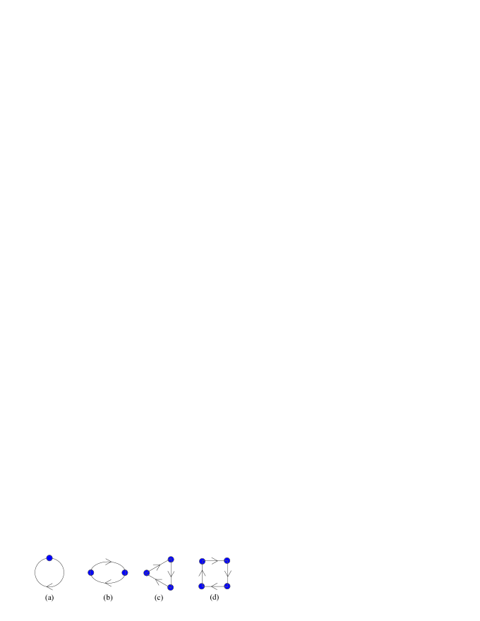
Figure 1:

Figure 2:

Table captions

Table 1.	Elements of the matrix $b$, describing mixing in the scalar isoscalar sector. The singlet-octet and quarkonia-glueball mixing effects are taken into account.
Table 2.	The model and experimental masses of scalar isoscalar meson states.
Table 3.	The partial and total decay widths (in MeV) of scalar isoscalar meson states. (∗)For the meson state $\sigma_{\rm II}$, there is possible a decay into kaons, which we did not calculate here, because its mass is at the threshold. We show only the lowest limit for its total decay width allowing for the decay into kaons that can increase the total decay width. The value is given for the model mass 1070 MeV. Next, in brackets, we also give the decay width calculated for the experimental mass 980 MeV. In the case of $\sigma_{\rm III}$, two values are given for its model mass and (in brackets) for the lowest bound for its experimental mass (1200 MeV).
Table 4.	Mixing coefficients for the ground and excited pion states.
Table 5.	Mixing coefficients for the ground and excited kaon states.
Table 6.	Mixing coefficients for the ground and excited $\eta$ and $\eta^{\prime}$ states. Here, the singlet-octet mixing is taken into account.

Tables

	$\sigma_{\rm I}$	$\sigma_{\rm II}$	$\sigma_{\rm III}$	$\sigma_{\rm IV}$	$\sigma_{\rm V}$
$\sigma_{8,1}$	0.973	0.137	0.393	0.548	0.048
$\sigma_{8,2}$	$-0.064$	0.204	$-0.978$	$-0.647$	$-0.047$
$\sigma_{9,1}$	$-0.225$	0.876	0.160	0.011	0.628
$\sigma_{9,2}$	$0.025$	0.146	0.136	$-0.082$	$-1.09$
$\chi^{\prime}$	$-0.266$	0.095	$-0.495$	$0.813$	$-0.116$

Table 1:

	Theor.	Exp. [4]
$\sigma_{\rm I}$	400	408 [24], 387 [25]
$\sigma_{\rm II}$	1070	980$\pm$10
$\sigma_{\rm III}$	1320	1200–1500
$\sigma_{\rm IV}$	1550	1500$\pm$10
$\sigma_{\rm V}$	1670	1712$\pm$5

Table 2:

	$f_{0}(400-1200)$	$f_{0}(980)$	$f_{0}(1370)$	$f_{0}(1500)$	$f_{0}(1710)$
$\pi\pi$	600	36 (20)	680 (480)	100	0.3
$K\bar{K}$	–	–	260 (125)	28	250
$\eta\eta$	–	–	62 (26)	4	20
$\eta\eta^{\prime}$	–	–	–	–	100
$4\pi(2\sigma_{\rm I})$	–	–	40	200	1
$\Gamma_{\rm tot}$	600	$>40(>20)(^{*})$	1040 (670)	330	370
$\Gamma_{\rm tot}^{\rm exp}$	600–1200	40–100	200–500	112$\pm$10	133$\pm$14

Table 3:

	$\pi$	$\pi^{\prime}$
$\pi_{1}$	0.997	0.511
$\pi_{2}$	0.007	$-$1.12

Table 4:

	$K$	$K^{\prime}$
$K_{1}$	0.954	0.533
$K_{2}$	0.102	$-$1.09

Table 5:

	$\eta$	$\eta^{\prime}$	$\hat{\eta}$	$\hat{\eta}^{\prime}$
$\phi_{8,1}$	0.777	$-0.359$	0.668	0.276
$\phi_{8,2}$	0.102	$-0.330$	$-1.03$	$-0.274$
$\phi_{9,1}$	0.546	0.701	$-0.010$	$-0.602$
$\phi_{9,2}$	0.037	0.225	$-0.333$	0.994

Table 6: