CERN–TH/2000–189 LPTHE–01–07 hep-ph/0102343 February 2001 Hadron masses and power corrections to event shapes

Abstract

It is widely believed that hadronisation leads to $1/Q$ corrections to $e^{+}e^{-}$ event shapes. We show that there are further corrections, proportional to $(\ln Q)^{A}/Q$ with $A=4C_{A}/\beta_{0}\simeq 1.6$, associated with hadron masses and whose relative normalisations can be calculated from one observable to another. At today’s energies these extra corrections can be of the same order of magnitude as ‘traditional’ $1/Q$ corrections. They fall into two classes: universal and non-universal. The latter can be eliminated by suitable redefinitions of the observables.

1 Introduction

For many non-perturbative aspects of QCD, there exist well defined methods of study such as lattice calculations or chiral perturbation theory. But one of the most fundamental aspects of non-perturbative QCD at high energy colliders, namely hadronisation, the relation between what is calculated perturbatively (parton level) and what is actually measured (hadron level) remains well beyond the reach of such methods. At best there are complex models which appear to reproduce much of the experimental data, but they leave something to be desired in terms of a fundamental understanding of what is involved in hadronisation.

Over the past few years there has been considerable theoretical [1, 2, 3, 4, 5, 6, 7, 8, 9, 10, 11, 12, 13, 14, 15, 16, 17, 18] and experimental [19, 20, 21, 22] interest in the study of hadronisation contributions to $e^{+}e^{-}$ and DIS event shapes. These variables provide a convenient ‘laboratory’ for such studies because the hadronisation effects are responsible for a significant fraction of the observable, making it feasible to carry out quantitative tests of the theoretical predictions.

A number of the current theoretical approaches are based on the idea of extending the reach of perturbation theory to very low scales — thus hadronisation effects are argued to be related to the infrared behaviour of the coupling, or equivalently to the high-order behaviour of the perturbative series. All the methods predict that the hadronisation (or power) corrections to event shapes should scale as $1/Q$, where $Q$ is the hard scale of the process. They also aim to predict the relative normalisation of the corrections from one observable to another.

As a result of their perturbative origins, the theoretical calculations are usually carried out with the assumption that all particles are massless. But in practice the observed hadrons do have masses. So in this paper we examine how the treatment of hadron masses modifies one’s expectations about power corrections.

It is perhaps worth illustrating how masses can affect our observables with a simple example. Let us consider the event-shape variable $\rho$, i.e. the squared invariant jet mass, normalised to $Q^{2}$ (for brevity we often refer to it simply as the jet mass). Initially one might consider a Born event consisting of a pair of back-to-back particles, each of mass $m$. The jet mass has the value $\rho=m^{2}/Q^{2}$. If this were the end of the story then we would argue that particle masses can be neglected since they give a $1/Q^{2}$ correction.

But one also needs to consider events containing soft particles. Here the situation is qualitatively different: the jet mass is $(E^{2}-p^{2})/Q^{2}$, where $E$ and $p$ are the total jet energy and $3$-momentum respectively. For a jet aligned along the $z$-axis a particle with mass $m_{i}$, $z$-momentum $p_{zi}$ and energy $E_{i}$ contributes an amount $(E_{i}-p_{zi})/Q$ to the jet mass and this difference includes a piece of order $m_{i}^{2}/(2E_{i}Q)$. For a soft particle with $E_{i}\sim\Lambda$ this translates to a $1/Q$ contribution. So parametrically at least, mass-related effects from soft particles are of the same order as traditional power corrections, and should not be neglected.

This is not the end of the story, for the simple reason that an event generally contains many soft particles: there will be a multiplicity-related enhancement of the $m^{2}/QE_{i}$ correction. The sum, over all particles, of $1/E_{i}$ is proportional to the $(-1)^{\mathrm{th}}$ moment of particle energy fractions. It has been known for a long time that positive moments and even the zeroth moment of particle energy fractions undergo logarithmic scaling violations with perturbatively calculable anomalous dimensions. It turns out that such analyses can be extended to negative moments, with the result that the sum $\sum_{i}1/E_{i}$ scales as $(\ln Q)^{A}$, where $A=4C_{\mathrm{A}}/\beta_{0}\simeq 1.6$, with $\beta_{0}=(11C_{\mathrm{A}}-2n_{\mathrm{f}})/3$. This means that the formally $1/Q$ contribution from mass effects is enhanced by a factor $(\ln Q)^{A}$.

The jet mass is an example of a variable in which it is quite straightforward to see that there are mass effects; in other cases the mass dependence can arise more subtly. For a general variable, the ability to factorise transverse and longitudinal degrees of freedom (with respect to the quark-antiquark directions) is an essential element of traditional, ‘perturbative’ approaches to hadronisation corrections. We will discover that for an ensemble of massive particles, differences arise between the factorisations applying to the event-shapes on the one hand and particle production on the other — and by studying this mismatch we become sensitive to hadron mass effects.

We will also see that a given event-shape variable can be defined in variety of ways (schemes) which are all equivalent for an ensemble of massless particles, but differ if there are massive particles. Two examples are a definition in terms of just $3$-momenta ($p$-scheme), and a definition in terms of energies and angles ($E$-scheme). It turns out that of these schemes, one, the $E$-scheme, is privileged, because it has the property that there is no mismatch between the event-shape and particle-production factorisation properties, even for massive ensembles.

Does this mean that in the $E$-scheme there are no mass-dependent contributions? The answer is no: it just means that any mass-dependent contribution is proportional to the same coefficient $c_{\cal V}$ as the ‘traditional’ non-perturbative correction. One can demonstrate that there really are still mass-dependent corrections by studying the difference between an event shape before hadrons have had the time to decay and after they have decayed.

We shall present the different elements of our analysis as follows. In section 2 we define the event shapes that will be considered and then quote their soft limits, being careful to leave in the leading dependence on particle masses.

Then in section 3 we review the tube model for non-perturbative effects [23, 2], which is known to reproduce all basic predictions for universal power corrections. However in contrast to previous treatments we leave in mass effects and see how they lead to non-universal $1/Q$ power corrections. This lays the ground for introducing alternative definitions of event shapes (massive, $p$, $E$ and decay-scheme definitions) which are identical for massless ensembles but differ in the treatment of particle masses.

Whereas the tube model is adequate for describing normal $1/Q$ power corrections it cannot address issues such as the scaling violations of energy moments which must be considered in order to derive the full $Q$-dependence of the mass-dependent corrections. For this we need to recall how coherent branching [24] affects hadron multiplicities and relate this to our particular problem. This is done in section 4.

Then in section 5 we start to study some of the practical aspects of mass corrections — for example we examine how, numerically, they compare to other contributions. We discuss some of the issues related to the experimental measurement of mass effects (a fairly difficult task) and we compare our predictions to results from Monte Carlo event generators. There is good agreement with Herwig [25] and Ariadne [26], but significant disagreement with Pythia [27] concerning the energy dependence of mass effects at very high energies.

Finally in section 6 we use a Monte Carlo event-generator to correct data for event shapes to a variety of schemes and see how this affects the fitted values for the perturbative and non-perturbative parameters $\alpha_{\mathrm{s}}$ and $\alpha_{0}$. We also investigate the feasibility of carrying out fits with an extra parameter intended to allow a separation of hadronisation into ‘traditional’ hadronisation effects and mass-related effects.

Our conclusions [28] are presented in section 7. The appendices contain a summary of the notation used and introduced in this article (appendix A), some calculational details related to the jet broadenings (appendix B), some considerations about $1/Q^{2}$ power corrections associated with heavy quark decay (appendix C), and a Monte-Carlo study of some peculiar features of the heavy-jet mass (appendix D).

2 Event shapes

The basic event shapes that we shall consider are the thrust $T$, the invariant jet mass $\rho$, the $C$-parameter and the total jet broadening $B_{T}$. For an ensemble of particles with momenta $k_{i}$ they are defined as follows:

$$T =\max_{\vec{n}}\frac{\sum_{i}\vec{k}_{i}.\vec{n}}{\sum_{i}|{\vec{k}}_{i}|}\,,$$ (2.1a)

$$\rho =\frac{\left(\sum_{i}k_{i}\,\Theta(\vec{k}_{i}.\vec{n}_{T})\right)^{2}}{\left(\sum_{i}k_{0i}\right)^{2}}\,.$$ (2.1b)

$$C =\frac{3}{2}\frac{\sum_{i,j}|{\vec{k}}_{i}||{\vec{k}}_{j}|\sin^{2}\theta_{ij}}{\left(\sum_{i}|{\vec{k}}_{i}|\right)^{2}}\,,$$ (2.1c)

$$B_{T} =\frac{\sum_{i}|{\vec{k}}_{ti}|}{2\sum_{i}|{\vec{k}}_{i}|}\,,$$ (2.1d)

where $\theta_{ij}$ is the angle between particles $i$ and $j$, $k_{i}=(k_{0i},\vec{k}_{i})$ the four-momentum, and ${\vec{k}}_{ti}$ the transverse momentum of particle $i$ with respect to the thrust axis $\vec{n}_{T}$.

We shall also discuss the heavy-jet mass $\rho_{h}$ which measures the invariant jet mass in the heavier of the two hemispheres (separated by the plane perpendicular to the thrust axis), and the wide-jet broadening $B_{W}$, which measures the jet-broadening in the wider of the two hemispheres.

For the purpose of calculating power corrections we will be interested in the behaviour of the event shapes variables for two-jet configurations, since it is such configurations which are the most frequent, representing a fraction $1-{\cal O}\left(\alpha_{\mathrm{s}}\right)$ of all events. In the two-jet limit all variables tend to zero, except the thrust which tends to $1$. Accordingly it will be more convenient to refer to $\tau=1-T$.

Essentially a two-jet event consists of a pair of back-to-back hard particles (which may have fragmented collinearly) and a bunch of accompanying soft particles. The hard particles (associated with the $q{\bar{q}}$ pair at parton level) define the axis of the event, while the soft particles (gluons at parton level) give the deviation of the event shape variable from its Born value of zero. Variables like $\tau$, $\rho$ and $C$ are particularly simple (linear) in that, in the two-jet limit their value is given by the sum of independent contributions from each soft particle:

$$\tau \simeq\frac{1}{Q}\sum_{i\in\mathrm{soft}}k_{ti}\,e^{-|{\bar{\eta}}_{i}|}\,,$$ (2.2a)

$$\rho \simeq\frac{1}{Q}\sum_{i\in\mathrm{soft}}\sqrt{k_{ti}^{2}+m_{i}^{2}}\,e^{-\eta_{i}}\,\Theta(\eta_{i})\,,$$ (2.2b)

$$C \simeq\frac{1}{Q}\sum_{i\in\mathrm{soft}}\frac{3\,k_{ti}}{\cosh{\bar{\eta}}_{i}}\,,$$ (2.2c)

where $${\bar{\eta}}_{i} i z {\bar{\eta}}_{i}=-\ln\tan\theta_{i}/2 \eta_{i} \eta_{i}=\frac{1}{2}\ln\frac{k_{0i}+k_{zi}}{k_{0i}-k_{zi}} \tau T \tau {\cal O}\left(\alpha_{\mathrm{s}}\right) {\cal O}\left(\Lambda\right) {\cal O}\left(\alpha_{\mathrm{s}}\Lambda/Q\right)$$ is the pseudorapidity of particle with respect to the thrust () axis, and is its rapidity . For massless particles the pseudorapidity and the rapidity are identical. In these expressions we have neglected mass effects in the denominators (in the case of , only after going from to ), since on average the numerator is small, , and thus modifications of to the denominator give effects of , which we can neglect.

Other variables like the heavy-jet mass and the broadenings are more complex. To see why, let us consider the case of the heavy-jet mass: when the event contains exactly one soft particle the heavy-hemisphere is always that in which the soft particle is present and the soft particle always contributes to the heavy jet mass. But if there are many soft particles then the hardest one (specifically, the one with the largest $k_{ti}\,e^{-|{\bar{\eta}}_{i}|}$) determines which hemisphere is heavy and any given softer particle contributes when it is in the heavy hemisphere i.e. only half the time. Thus the heavy jet mass is not equal to a linear combination of independent contributions from each soft particle.

For the purposes of studying non-perturbative corrections we can however make a simplifying approximation: the ‘hardest’ soft particles come from perturbative emissions, while non-perturbative emissions will be much softer. The contributions from these softest particles do combine linearly [7, 12], so that one can write

$$\rho_{h}\simeq\frac{1}{Q}\sum_{i\in\mathrm{softest}}\sqrt{k_{ti}^{2}+m_{i}^{2}}\,e^{-\eta_{i}}\,\Theta(\eta_{i})+\ldots\,,$$ (2.2d)

where we have taken the hard hemisphere as being that with $\eta>0$ and the dots indicate the contribution from harder particles. For both jet broadenings analogous arguments apply [12, 15] and one has

$$B_{T} \simeq\frac{1}{2Q}\sum_{i\in\mathrm{softest}}k_{ti}\,+\ldots$$ (2.2e)

$$B_{W} \simeq\frac{1}{2Q}\sum_{i\in\mathrm{softest}}k_{ti}\,\Theta({\bar{\eta}}_{i})+\ldots\,,$$ (2.2f)

where again we have taken the wide hemisphere as being that with ${\bar{\eta}}>0$.

3 Power corrections: the tube model

A variety of approaches exist for the study of power corrections in event shapes [1, 2, 3, 4, 5, 6, 7, 8, 9, 10, 11, 12, 13, 14, 15, 16, 17, 18]. The simplest, which reproduces the results of the more sophisticated methods [10, 11, 12, 13, 14], is the tube, or longitudinal phase-space model [23, 2].

The principle behind the tube model (the ideas of [6] are analogous, though presented in a more formal language) is as follows. Soft hadrons (i.e. the hadrons responsible for non-perturbative corrections) are generated from the $q{\bar{q}}$ pair of sources; since both sources are fast moving (in opposite directions) a moderate boost along the $q{\bar{q}}$ direction still leaves us with two fast-moving particles, and so does not change the structure of the low-transverse momentum fields at central rapidities. As a result soft particle production at central rapidities must be boost-independent. Since a boost just corresponds to a shift in rapidity, this is equivalent to saying that non-perturbative (and in general soft) particle production is rapidity-independent, at least for rapidities $\eta\ll\ln Q/k_{t}$, beyond which one becomes sensitive to the finite energy of the source. The tube model makes no statement about the transverse-momentum distribution of soft particles, so we just write the distribution of non-perturbatively produced hadrons of type $h$ as being:

$$\frac{dn_{h}}{d\eta\,d\ln k_{t}}=\phi_{h}(k_{t}),\qquad|\eta|\ll\ln\frac{Q}{k_{t}}\,,$$ (3.1)

with $\phi_{h}(k_{t})$ some a priori unknown function. There is no $Q$-dependence in $\phi_{h}(k_{t})$ since the fields generated by a source ($q$ or ${\bar{q}}$) moving close to the speed of light are independent of the energy of the source.

3.1 Massless case

Most power correction analyses work within the approximation that particles are massless. As a result in eqs. (2.2) all explicit mass-dependence disappears, and one can replace ${\bar{\eta}}$ with $\eta$. This leaves the expressions for the event-shape variable ${\cal V}$ in a factorised form, whereby all rapidity dependence (which differs from one observable to another) can be separated from the transverse momentum dependence ($k_{t}/Q$ in all observables):

$${\cal V}=\sum_{i\in\mathrm{soft}}\frac{k_{ti}}{Q}f_{\cal V}(\eta_{i})\,.$$ (3.2)

For example for the the thrust we have $f_{\tau}(\eta)=e^{-|\eta|}$. The non-perturbative contribution to the mean value of the event-shape is then given by

$$\langle{\cal V}_{\mathrm{NP}}\rangle=\int\frac{dk_{t}}{k_{t}}\,\frac{k_{t}}{Q}\sum_{h}\phi_{h}(k_{t})\int d\eta f_{{\cal V}}(\eta)\;=\;\frac{a_{0}}{Q}\,c_{{\cal V}}$$ (3.3)

where we have defined a non-perturbative parameter

$$a_{0}=\int dk_{t}\sum_{h}\phi_{h}(k_{t})$$ (3.4)

and a calculable, variable-dependent coefficient,

$$c_{{\cal V}}=\int d\eta\,f_{{\cal V}}(\eta)\,.$$ (3.5)

The factorisation of rapidity and $k_{t}$ dependence is the prerequisite for universality, namely the fact that the power corrections for a range of observables all depend on the same, universal, non-perturbative quantity ($a_{0}$), with a calculable coefficient ($c_{\cal V}$). The predictions for the coefficients are given in table 1.

${\cal V}$	$\tau$	$\rho$	$\rho_{h}$	$C$	$B_{T}$	$B_{W}$
$c_{\cal V}$	$2$	$1$	$1$	$3\pi$	$\frac{\pi}{2\sqrt{C_{F}\alpha_{\mathrm{s}}}}-\frac{\beta_{0}}{6C_{\mathrm{F}}}+\eta_{0}$	$\frac{\pi}{4\sqrt{2C_{F}\alpha_{\mathrm{s}}}}-\frac{\beta_{0}}{24C_{\mathrm{F}}}+\frac{\eta_{0}}{2}$

Table 1: coefficients of $1/Q$ power corrections; $\beta_{0}=\frac{11}{3}C_{\mathrm{A}}-\frac{2}{3}n_{\mathrm{f}}$ and $\eta_{0}\simeq 0.13629$.

The more complex form for the broadenings [15] arises because these variables are sensitive to the mismatch between the thrust axis and the quark axis. Emissions are uniform in rapidity with respect to the latter, whereas the broadening measures $k_{t}$ with respect to the former. After considering recoils one finds that there is an effective cutoff on contributions from rapidities (with respect to the thrust axis) $\eta\gtrsim\ln Q/p_{t}$, where $p_{t}$ is the transverse momentum of the quark with respect to the thrust axis. This leads to $c_{B}\sim\langle\ln Q/p_{t}\rangle$ which is of the order of $1/\sqrt{\alpha_{\mathrm{s}}}$.

More sophisticated approaches to the problem of power corrections at first sight seem quite different from the tube model: they examine the high-order behaviour of the perturbation series, or the dependence of the observable on a dispersive gluon virtuality (see for example [3, 4, 7, 8]). But it turns out that both of these procedures are equivalent to determining the dependence of the observable on infra-red properties of the coupling; since the production of gluons with a given $k_{t}$ is rapidity-independent and proportional to $\alpha_{\mathrm{s}}(k_{t}$) we have a situation very similar to the tube model but with $\phi_{h}(k_{t})$ replaced with $\alpha_{\mathrm{s}}(k_{t})$. Accordingly we can write a relation between $a_{0}$ and the quantity $\alpha_{0}(\mu_{I})$, often used in phenomenological analyses, defined as

$$\alpha_{0}(\mu_{I})\equiv\int_{0}^{\mu_{I}}\frac{dk_{t}}{\mu_{I}}\>\alpha_{\mathrm{s}}(k_{t})\>,$$ (3.6)

namely [3, 4, 11, 12]

$$\frac{a_{0}}{Q}=\frac{4C_{F}}{\pi^{2}}{\cal M}\frac{\mu_{I}}{Q}\left\{\alpha_{0}(\mu_{I})-\alpha_{\mathrm{s}}(Q)-\beta_{0}\frac{\alpha_{\mathrm{s}}^{2}}{2\pi}\left(\ln\frac{Q}{\mu_{I}}+\frac{K}{\beta_{0}}+1\right)\right\}$$ (3.7)

with ${\cal M}\simeq 1.490$, $K=C_{\mathrm{A}}\left(\frac{67}{18}-\frac{\pi^{2}}{6}\right)-\frac{5}{9}n_{\mathrm{f}}$. The purpose of the $\alpha_{\mathrm{s}}$ terms in (3.7) is to subtract out contributions that are already taken into account in the perturbative calculation of the mean value.

It has become a standard procedure to carry out simultaneous fits for $\alpha_{\mathrm{s}}$ and $\alpha_{0}$ in mean values of a variety of event shapes. One important test of this class of models for hadronisation corrections is then that the fitted values $\alpha_{0}$ (and $\alpha_{\mathrm{s}}$) should be the same for all variables, i.e. that $\alpha_{0}$ should be universal.

3.2 Including mass effects

From the point of view of the tube model itself nothing changes when one introduces masses for the hadrons — we still have a distribution of hadrons independent of rapidity and with some unknown dependence on $k_{t}$. What does change is that we need to use the full (massive) expressions for the values of the event shapes. In most cases the event shapes are just defined in terms of the pseudorapidities (angles) and transverse momenta of the particles. This means that we have to keep track of the relation between rapidity and pseudorapidity, which is expressed in the following (equivalent) equations:

$$k_{t}\sinh{\bar{\eta}} =\sqrt{k_{t}^{2}+m^{2}}\sinh\eta\,,$$ (3.8a)

$$k_{t}^{2}\cosh^{2}{\bar{\eta}}+m^{2} =(k_{t}^{2}+m^{2})\cosh^{2}\eta\,.$$ (3.8b)

For example for the thrust and the $C$-parameter, we have

$$\langle{\cal V}_{\mathrm{NP}\mathrm{-massive}}\rangle=\int\frac{dk_{t}}{k_{t}}\,\frac{k_{t}}{Q}\sum_{h}\phi_{h}(k_{t})\;\int d\eta\,f_{{\cal V}}\left({\bar{\eta}}\left(\eta,\frac{m_{h}^{2}}{k_{t}^{2}}\right)\right)$$ (3.9)

where all that has changed compared to eq. (3.3) is the replacement of $f_{\cal V}(\eta)$ with $f_{\cal V}({\bar{\eta}})$. However the fact that ${\bar{\eta}}$ is a function of both $\eta$ and $m^{2}/k_{t}^{2}$ means that eq. (3.9) cannot be factorised into two independent pieces. Hence universality (a direct consequence of the factorisation) is broken.

For a general variable ${\cal V}$ it will be convenient to write the resulting non-universal mass-dependent piece of the power correction as

$$\langle\delta_{m}{\cal V}\rangle=\int\frac{dk_{t}}{k_{t}}\,\frac{k_{t}}{Q}\sum_{h}\phi_{h}(k_{t})\;\int d\eta\;\delta f_{{\cal V}}\!\left(\eta,\frac{m_{h}^{2}}{k_{t}^{2}}\right)\,,$$ (3.10)

where for example, for the thrust

$$\delta f_{\tau}\!\left(\eta,\frac{m^{2}}{k_{t}^{2}}\right)=f_{\tau}({\bar{\eta}})-f_{\tau}(\eta)=e^{-|{\bar{\eta}}|}-e^{-|\eta|}\,.$$ (3.11)

We then proceed in a manner analogous to that in the massless case. We define a $\delta c_{\cal V}$,

$$\delta c_{{\cal V}}\left(\frac{m^{2}}{k_{t}^{2}}\right)=\int d\eta\,\delta f_{{\cal V}}\!\left(\eta,\frac{m^{2}}{k_{t}^{2}}\right)\,,$$ (3.12)

which unlike $c_{\cal V}$ depends on $k_{t}$ (a consequence of the non-factorisability). Then the mass-dependent correction to the mean value of the event shape is

$$\langle\delta_{m}{\cal V}\rangle=\sum_{h}\frac{m_{h}}{Q}\int\frac{dk_{t}}{k_{t}}\,\phi_{h}(k_{t})\;\frac{k_{t}}{m_{h}}\,\delta c_{{\cal V}}\left(\frac{m_{h}^{2}}{k_{t}^{2}}\right)\,.$$ (3.13)

To understand the properties of the mass-dependent corrections we need to study the $\delta c_{\cal V}$’s:

$$\delta c_{\cal V}\left(\frac{m^{2}}{k_{t}^{2}}\right)=\left\{\begin{array}[c]{ll}\displaystyle\int d{\bar{\eta}}\,f_{{\cal V}}({\bar{\eta}})\,\left(\frac{d\eta}{d{\bar{\eta}}}-1\right)&{\cal V}=\tau,C,B_{T},B_{W},\vspace{0.2cm}\\ \displaystyle\int d\eta\,e^{-\eta}\,\Theta(\eta)\left(\sqrt{1+m^{2}/k_{t}^{2}}-1\right)&{\cal V}=\rho,\rho_{h}\,,\end{array}\right.$$ (3.14)

where

$$\frac{d\eta}{d{\bar{\eta}}}=\frac{\cosh{\bar{\eta}}}{\sqrt{\cosh^{2}{\bar{\eta}}+m^{2}/k_{t}^{2}}}\,.$$ (3.15)

For the event-shapes in the first line of eq. (3.14) the integrals have been rewritten with a change of variable in the first term as this simplifies their subsequent evaluation.

The exact forms for the $\delta c_{\cal V}$ are

$$\delta c_{\tau}\left(\frac{m^{2}}{k_{t}^{2}}\right) =2\left[\frac{1}{\xi}\,\mathbf{K}\!\left(\frac{\sqrt{\xi^{2}-1}}{\xi}\right)-\xi\mathbf{E}\!\left(\frac{\sqrt{\xi^{2}-1}}{\xi}\right)+\xi-1\right],$$ (3.16a)

$$\delta c_{C}\left(\frac{m^{2}}{k_{t}^{2}}\right) =\frac{6}{\xi}\,\mathbf{K}\!\left(\frac{\sqrt{\xi^{2}-1}}{\xi}\right)-3\pi\,,$$ (3.16b)

$$\delta c_{B_{T}}\left(\frac{m^{2}}{k_{t}^{2}}\right) =2\delta c_{B_{W}}=-\ln\xi\,,$$ (3.16c)

$$\delta c_{\rho}\left(\frac{m^{2}}{k_{t}^{2}}\right) =\delta c_{\rho_{h}}=\xi-1\,,$$ (3.16d)

where we have introduced the shorthand $\xi^{2}=1+m^{2}/k_{t}^{2}$, and $\mathbf{E}$ and $\mathbf{K}$ are the complete elliptic integrals defined as follows,

$$\mathbf{E}(x) =\int_{0}^{\pi/2}\sqrt{1-x^{2}\sin^{2}\psi}\;d\psi\qquad(|x|\leq 1)\,,$$ (3.17a)

$$\mathbf{K}(x) =\int_{0}^{\pi/2}\frac{d\psi}{\sqrt{1-x^{2}\sin^{2}\psi}}\qquad\quad\;(|x|<1)\,.$$ (3.17b)

To see how the $\delta c_{\cal V}$ will affect our power correction we compare them to the universal $c_{\cal V}$ power contribution. Figure 1 shows $[c_{\cal V}+\delta c_{\cal V}(m^{2}/k_{t}^{2})]/c_{\cal V}$ for a range of variables as a function of $k_{t}/m$. One immediately sees that for small $k_{t}$ the non-perturbative correction to the jet mass will be enhanced, while the NP correction to the other variables will be suppressed. Furthermore the enhancement for the jet mass is much larger than the suppression for the other variables (which are fairly similar to one another).

Figure 1: The dependence of $c_{\cal V}+\delta c_{\cal V}$ on particle masses, shown for the four distinct groups of variables.

${\cal V}$	$\tau$	$\rho$	$\rho_{h}$	$C$	$B_{T}$	$B_{W}$
$\gamma_{\cal V}$	$-\pi/2$+1	$1/2$	$1/2$	$-3\pi/4$	$-1/2$	$-1/4$
$\gamma_{\cal V}/c_{\cal V}$	$-0.285$	$0.5$	$0.5$	$-0.25$	$-0.180$	$-0.227$

Table 2: The coefficients of the high-$k_{t}$ behaviour of the mass-dependent power correction, $\gamma_{\cal V}$. In the case of the broadenings the $c_{\cal V}$ depend on $\alpha_{\mathrm{s}}(Q)$, so the ratio $\gamma_{\cal V}/c_{\cal V}$ is shown for $Q=M_{Z}$.

To study the question more quantitatively we observe that for large $k_{t}$, the $\delta c_{\cal V}$ scale as $m^{2}/k_{t}^{2}$,

$$\delta c_{\cal V}\left(\frac{m^{2}}{k_{t}^{2}}\right)=\gamma_{\cal V}\frac{m^{2}}{k_{t}^{2}}+{\cal O}\left(\frac{m^{4}}{k_{t}^{4}}\right)$$ (3.18)

with the $\gamma_{\cal V}$ given in table 2. This means that the integral in eq. (3.13) is dominated by low momenta for all reasonable forms of the distribution of particles $\phi_{h}(k_{t})$, and hence just gives a number. Therefore $\langle\delta_{m}{\cal V}\rangle$ is proportional to $1/Q$, i.e. formally of the same order as the universal power correction.

The question of the quantitative relationship between the sizes of the mass-corrections in the different observables is more delicate because it depends on the region of $k_{t}$ which dominates the integral in eq. (3.13). If $\phi(k_{t})$ is such that moderate $k_{t}$’s dominate (i.e. where $\delta c_{\cal V}$ is equal to $\gamma_{\cal V}m^{2}/k_{t}^{2}$) then we can expect the following relation to hold:

$$\langle\delta_{m}{\cal V}\rangle\propto\gamma_{\cal V}\,.$$ (3.19)

If $\phi(k_{t})$ is such that smaller $k_{t}$’s dominate the integral (3.13), then formally we can make no such statement. Nevertheless by examining figure 2, which shows $k_{t}/m\delta c_{\cal V}/\gamma_{\cal V}$ as a function of $k_{t}/m$, one observes that for $\tau$, $C$ and the broadenings the shape of the $\delta c_{\cal V}(m^{2}/k_{t}^{2})$ functions are very similar. This means that regardless of the form of $\phi(k_{t})$ we will still observe the property that

$$\frac{\langle\delta_{m}{\cal V}_{1}\rangle}{\gamma_{{\cal V}_{1}}}\simeq\frac{\langle\delta_{m}{\cal V}_{2}\rangle}{\gamma_{{\cal V}_{2}}}\,.$$ (3.20)

For the jet masses on the other hand, $\delta c_{\cal V}(m^{2}/k_{t}^{2})$ has a different shape and being considerably larger at small momenta, so that we can expect the following relation to hold:

$$\frac{\langle\delta_{m}\rho\rangle}{\gamma_{\rho}}\gtrsim\frac{\langle\delta_{m}\tau\rangle}{\gamma_{\tau}}\,.$$ (3.21)

Figure 2: The observable-dependent piece of the integrand for the non-universal mass-dependent power correction, eq. (3.13), normalised to $\gamma_{\cal V}$. The curve labelled ‘decay’ will be discussed in section 3.4.

The conclusion of this section is that mass effects introduce extra $1/Q$ power corrections, which break the simple ‘universal’ picture of power corrections that is obtained in the massless case. For most variables we expect a negative correction, whose magnitude is roughly proportional to $\gamma_{\cal V}$ (which for these variables is roughly $-c_{\cal V}/4$). For the jet masses we expect positive corrections whose magnitude is larger than what would be expected from a simple proportionality to $\gamma_{\cal V}$ (which itself is $c_{\cal V}/2$) .

3.3 Alternative schemes

So far we have used the event-shape definitions given in eqs. (2.1). From the point of view of the perturbative QCD calculation however we could have chosen any number of related definitions with the same massless limit and we would have obtained the same perturbative (and universal non-perturbative) predictions. Here we discuss two particular examples of such modifications.

The $\boldsymbol{p}$-scheme:

The difference between the jet masses and the other variables occurs because the jet masses are the only variables to be sensitive to the difference between the energies and 3-momenta of the particles. However one could equally well consider a second pair of variables, identical to the jet masses except that they are defined only in terms of the particle 3-momenta (i.e. in the definition, each occurrence of particle energy is replaced by the modulus of the corresponding 3-momentum). We will refer to these as the jet masses in the $p$-scheme (whereas we will refer to the default definitions as the massive scheme).

As pointed out at the beginning of the section, from the point of view of the perturbative and universal non-perturbative calculations, which ignore particle masses, such a variable would have identical properties to the original jet mass. However, for an event consisting of soft massive particles its value would be

$$\rho_{p}\simeq\frac{1}{Q}\sum_{i\in\mathrm{soft}}k_{ti}\,e^{-|{\bar{\eta}}_{i}|}\,\Theta({\bar{\eta}}_{i})\,,$$ (3.22)

rather than eq. (2.2b). Noting the similarity between this expression and eq. (2.2a), one obtains that

$$\frac{\delta c_{\rho_{p}}(m^{2}/k_{t}^{2})}{c_{\rho}}=\frac{\delta c_{\tau}(m^{2}/k_{t}^{2})}{c_{\tau}}\,,$$ (3.23)

i.e. relative to the universal power correction the mass-dependent piece is identical in the two cases. The use of the $p$-scheme makes no difference for the variables other than jet masses, since they are all already defined purely in terms of the 3-momenta.

So in the $p$-scheme all variables should have a mass-dependent correction which is roughly proportional to $\gamma_{\cal V}$, which itself is roughly proportional to $c_{\cal V}$. Therefore universality should (more or less) appear to remain intact.

The $\boldsymbol{E}$-scheme:

Another definition of event-shapes which is identical at the perturbative and universal non-perturbative level is one defined purely in terms of the energies and directions of particles, i.e. where all 3-momenta are substituted with momenta in the same direction but whose modulus is equal to the energy. We call this the $E$-scheme. We note that similar definitions, in terms of energy flow, have been suggested in the past by various authors [6, 29], on the grounds that they are closer to what is measured in a experimental calorimeter and that they may also allow event shapes to be expressed in terms of correlation function of fields.

The expression for $\rho_{E}$ in the soft limit is

$$\rho_{E}\simeq\frac{1}{Q}\sum_{i\in\mathrm{soft}}k_{ti}\,e^{-|{\bar{\eta}}_{i}|}\,\Theta({\bar{\eta}}_{i})\,\frac{\sqrt{\cosh^{2}{\bar{\eta}}_{i}+m^{2}_{i}/k_{ti}^{2}}}{\cosh{\bar{\eta}}_{i}}\,,$$ (3.24)

where the extra factor compared to $\rho_{p}$ is the ratio of the energy to the 3-momentum. The expression for $\delta c_{\rho_{E}}$ is then

$$\delta c_{\rho_{E}}\left(\frac{m^{2}}{k_{t}^{2}}\right)=\int d{\bar{\eta}}\,e^{-|{\bar{\eta}}|}\,\Theta({\bar{\eta}})\left(\frac{d\eta}{d{\bar{\eta}}}\cdot\frac{\sqrt{\cosh^{2}{\bar{\eta}}+m^{2}/k_{t}^{2}}}{\cosh{\bar{\eta}}}-1\right)\,.$$ (3.25)

However, noting the form of $d\eta/d{\bar{\eta}}$, eq. (3.15), one sees that this is identically zero. A similar phenomenon occurs for the other variables, i.e. in general we have

$$\delta c_{{\cal V}_{E}}\left(\frac{m^{2}}{k_{t}^{2}}\right)\equiv 0\,.$$ (3.26)

In other words in the $E$-scheme there is no non-universal mass-dependent $1/Q$ power correction. So if one wants to study the universality of $1/Q$ power corrections, the best to way to do it is to measure all variables in the $E$-scheme.

The $p$ and $E$-schemes are of also of interest because in principle one can measure the difference between a given observable in two different schemes. For example if one measures the difference between $\tau$ in the $p$ and $E$-schemes, one expects this to be equal to $\langle\delta_{m}\tau\rangle$. This can be done for various observables, after which one can verify the relations (3.20, 3.21).

3.4 Hadron decay

Quite often hadron-level measurements are performed on particles which are unstable, though long-lived compared to their time of flight across the detector. The definition of the observable does not specify at what stage of the hadron decay chain we should make our measurement, so we are actually free to make it at any stage we like — as long as we specify the stage.

This leads us to wonder about dependence of the observable on the particular hadron level that is chosen. It is possible quite generally to argue that redefining the hadron level should not affect the universality pattern. Suppose one starts off at a stage consisting of short-lived hadronic resonances. The boost-invariant nature of the mechanisms of hadronisation implies that these hadronic resonances will have been produced with a rapidity-independent distribution. Hadron decay is also a boost invariant process, so the decay products of the resonances will also be distributed in a rapidity-invariant manner. But the mean transverse momentum may well change because the decay of a hadron liberates energy, some of which may enter into the transverse degrees of freedom. Therefore the power correction to a given observable will increase as a result of hadron decay, but the increase will be proportional to $c_{\cal V}$ (as long as the observable is measured in the $E$-scheme).

Though it is perhaps more natural to treat hadron decay as a change in the distributions $\phi_{h}(k_{t})$, if one wants quantitative predictions it turns out to be more convenient to discuss it in terms of a $\delta c_{\cal V}(m^{2}/k_{t}^{2})$ contribution. Since our decay process is rapidity independent we can write the $\delta c_{{\cal V}_{\mathrm{decay}}}$ for an arbitrary variable as

$$\delta c_{{\cal V}_{\mathrm{decay}}}\left(\frac{m^{2}}{k_{t}^{2}}\right)=c_{\cal V}\,X_{\mathrm{decay}}\left(\frac{m^{2}}{k_{t}^{2}}\right)$$ (3.27)

where $X_{\mathrm{decay}}$, which is independent of the variable, is defined by

$$X_{\mathrm{decay}}\left(\frac{m^{2}}{k_{t}^{2}}\right)=\left\langle\frac{1}{k_{t}}\sum_{i\,\in\,\mathrm{children}}|k_{ti}|\right\rangle-1\,,$$ (3.28)

is the mean relative change in total transverse momentum as a result of the decay of a parent with transverse momentum $k_{t}$ and mass $m$.

In general $X_{\mathrm{decay}}$ is a fairly complicated function, because actual hadronic decays can involve 3-body final states where one or more of the decay products is massive. For the purposes of the studies in this paper we instead introduce a decay-scheme, in which all hadrons are artificially decayed to a pair of massless particles. At first sight this seems a little arbitrary, but there are two reasons why it is nevertheless of interest. Firstly, it is fairly straightforward to apply this scheme to a given ensemble of particles: one simply takes each hadron and in its centre of mass frame decays it to two particles moving in opposite directions along a randomly chosen axis. The second reason is phenomenological: as we shall discover in section 5.3 if one applies the procedure to different hadron levels (say the normal hadron level and some ‘resonance’ level, earlier on in the decay chain) one finds that the decay scheme results in the two cases are very similar — in other words, decay-scheme results are almost independent of the particular hadron level from which one starts.

In this 2-body decay scheme, $X_{\mathrm{decay}}$ is given by the following expression

$$X_{\mathrm{decay}}\left(\frac{m^{2}}{k_{t}^{2}}\right)=\\ \qquad\int_{-1}^{1}d(\cos\theta)\int_{0}^{2\pi}\frac{d\phi}{4\pi}\left(\sqrt{1+\left(\frac{m^{2}}{k_{t}^{2}}+\cos^{2}\phi\right)\sin^{2}\theta+2\sqrt{1+\frac{m^{2}}{k_{t}^{2}}}\sin\theta\cos\phi}-1\right),$$ (3.29)

for which we have yet to find a closed form. Its behaviour for $k_{t}\gg m$ is such that for a general variable the expansion coefficient defined in eq. (3.18) is

$$\gamma_{{\cal V}_{\mathrm{decay}}}=\frac{1}{4}c_{\cal V}\,.$$ (3.30)

The shape of the function $\delta c_{{\cal V}_{\mathrm{decay}}}$ is similar to that of $\delta c_{\rho}$, as can be seen from figure 2.

3.5 Relation to massive-gluon calculations

Many of the traditional power-correction calculations are based on the dispersive, or massive-gluon approach. Often however, as we have already mentioned, there is an implicit or even explicit [10, 11, 12, 13, 14] assumption that the gluon decays into massless particles, leading to the statement of universality.

One exception is the calculation in [8] which considered the thrust using the full kinematics of the undecayed massive gluon (both in the numerator, where gluon decay often makes no difference, and in the denominator where it does make a difference). They obtained the result that the coefficient $c_{\tau}$ for the thrust should be $4G$ rather than $2$, where $G\simeq 0.916$ is Catalan’s constant. This seems quite strange since we have argued that a proper treatment of particle masses should lower the value of the thrust rather than increase it, whereas the analysis of [8] suggests that the power correction increases. However the situation is subtle because the massive-gluon approach takes the power correction as being proportional to the non-analyticity in the gluon mass (or virtuality) after integration over the whole of phase space, and there is a non-trivial relation between the effect of the gluon mass on the value of $\tau$ for a given event and the non-analyticity.

4 QCD-based analysis

When discussing universal power corrections in section 3 we introduced the function $\phi_{h}(k_{t})$, the one-particle inclusive distribution for the non-perturbative production of hadrons $h$ with transverse momentum $k_{t}$. Within the tube model we vaguely know what we mean (the hadronisation associated with the low momentum fields from the $q,{\bar{q}}$ sources), but in QCD it is quite ambiguous: after all, all hadrons are produced non-perturbatively!

Strictly what we are interested in is the difference between our observable at the hadron level and the value calculated from a given order of perturbation theory. In our particular case the variables are sensitive to the mean transverse momentum (at a given rapidity). A proper definition of the difference in mean transverse momentum between parton and hadron levels is

$$a_{0}=\int\frac{dk_{t}}{k_{t}}k_{t}\left(\sum_{h}\Phi_{h}(k_{t},\eta)-\sum_{p=q,g}\Phi_{p}(k_{t},\eta)\right)$$ (4.1)

where $\Phi_{h}(k_{t},\eta)$ is the distribution of hadrons $h$ at a given transverse momentum and rapidity, and $\Phi_{q,g}(k_{t},\eta)$ is the perturbative distribution of partons. So the quantity $\phi_{h}(k_{t})$ should really be understood as being defined as follows:

$$\sum_{h}\phi_{h}(k_{t})\cong\sum_{h}\Phi_{h}(k_{t},\eta)-\sum_{p=q,g}\Phi_{p}(k_{t},\eta).$$ (4.2)

In eq. 4.1 the integrals over $\Phi_{h}(k_{t},\eta)$ or $\Phi_{q,g}(k_{t},\eta)$ separately would have values of the order of $\alpha_{\mathrm{s}}\,e^{-|\eta|}\,Q$, because a fraction $\alpha_{\mathrm{s}}$ of the time there can be a hard particle. But typical pictures of hadronisation state that the difference should be dominated by particles ‘produced at low transverse momenta,’ as opposed to particles which come from the collinear fragmentation of a hard parton, since in the latter case the sum of $k_{t}$’s of the hadrons should on average be equal to the $k_{t}$ of the original parton and there will be no contribution to the difference (4.1). This ensures that the integral of $\sum_{h}\phi_{h}$ is dominated by low $k_{t}$’s and that it is roughly rapidity and $Q$-independent.

But when working out mass-dependent effects, $\Phi_{q,g}$ does not contribute at all since in the perturbative calculation one has massless quarks and gluons (we do not consider the case of calculations with massive quarks). So in the expression for the mass-dependent non-universal power correction, eq. (3.9), we shall replace $\phi_{h}(k_{t})$ with $\Phi_{h}(k_{t},\eta)$.

4.1 Spectrum of hadrons

To study mass effects in detail it is necessary to have some understanding about $\Phi_{h}$. The simplest approach that is currently available is based on local parton-hadron duality (LPHD) [30, 31], namely the idea that on average there is a correspondence between the production of partons and the production of hadrons. One can then calculate the distribution of partons and expect the distribution of hadrons to be very similar. Using this idea the distribution of low-$k_{t}$ hadrons has been calculated as a function of $k_{t}$ and rapidity in [32]:

$$\Phi(k_{t},\eta,\ln Q/\Lambda)\sim\frac{4C_{\mathrm{F}}}{\beta_{0}}\left(\frac{1}{\ln k_{t}/\Lambda}+\frac{4C_{\mathrm{A}}}{\beta_{0}}\ln\frac{\ln k_{t}/\Lambda}{\ln Q_{0}/\Lambda}\ln\frac{\ln Qe^{-|\eta|}/\Lambda}{\ln k_{t}/\Lambda}+\cdots\right)$$ (4.3)

where $\Lambda$ is the QCD scale in some arbitrary scheme, $Q_{0}$ is an unknown cutoff below which parton branching stops. We have explicitly added $\ln Q$ as an argument of $\Phi$ to emphasise that it is now $Q$ dependent. The $\eta$ dependence of $\Phi$ is actually properly described by this formula only for large $\eta$. But since most of our integrals in $\eta$ converge rapidly we will usually be able to ignore the $\eta$-dependence altogether.

The first term in the brackets in (4.3) just corresponds to the radiation of a single gluon of transverse momentum $k_{t}$ from the $q{\bar{q}}$ pair, with intensity $\alpha_{\mathrm{s}}(k_{t})$. This term is both rapidity and $Q$-independent. The second term comes from the coherent (or angular ordered) radiation of another gluon from the first gluon, with the logarithms originating from the integrations over the two gluon momenta.

At lowest momenta the first term dominates. At higher momenta the second term becomes more important. We note that it has significant $Q$-dependence: this means that a piece of the mass-dependent correction will behave as $\ln\ln Q$ times some function of $k_{t}$, and the fact that this function is enhanced at larger values of $k_{t}$ implies sensitivity to $\delta c_{\cal V}(m^{2}/k_{t}^{2})$ in a region where the approximation of $\delta c_{\cal V}$ by $\gamma_{\cal V}\,m^{2}/k_{t}^{2}$ might be expected to work — in other words we expect there to be a term in the mass-dependent power correction proportional to

$$\gamma_{\cal V}\,\frac{\ln\ln Q/\Lambda}{Q}\,,$$

as opposed to a simple $1/Q$ correction.

A proper treatment requires that one take into consideration not only the first term to have $Q$ dependence in (4.3) but also yet higher orders. This can be done via moments $D_{\omega}(\ln Q)$ of the multiplicity distribution of particles with momentum fraction $x$ emitted from a gluon at scale $Q$, $D(x,\ln Q)$:

$$D_{\omega}(Y=\ln Q/\Lambda)=\int_{0}^{1}\frac{dx}{x}x^{\omega}\left[xD(x,Y)\right]\,.$$ (4.4)

The corresponding moment for emissions from a quark is just $C_{\mathrm{F}}/C_{\mathrm{A}}D_{\omega}(Y)$. We will actually be interested in the moments of the multiplicity distribution at fixed $\eta$ (which we take positive), $\Phi_{\omega}(\eta)$,

$$\Phi_{\omega}(\eta,\ln Q/\Lambda)=\int\frac{dk_{t}}{k_{t}}\left(\frac{k_{t}}{Q}\right)^{\omega}\Phi(k_{t},\eta,\ln Q/\Lambda)$$ (4.5)

which is given in terms of $D_{\omega}$ by

$$\Phi_{\omega}(\eta,\ln Q/\Lambda)=e^{-\omega\eta}\left.\frac{d}{dY}D_{\omega}(Y)\right|_{Y=\ln Q/\Lambda-\eta}\,.$$ (4.6)

The full multiplicity moment satisfies the following equation, embodying coherence [24] at double logarithmic accuracy (DLA) as discussed for example in [33]

$$\frac{d}{dY}D_{\omega}(Y)=\int_{0}^{\infty}dy\,e^{-\omega y}\,4C_{\mathrm{A}}\frac{\alpha_{\mathrm{s}}(Y-y)}{2\pi}D_{\omega}(Y-y)\,.$$ (4.7)

By differentiating both sides this can be written as a second order differential equation, for which an approximate (DLA) solution is

$$D_{\omega}(Y)\simeq D_{\omega}(Y_{0})\exp\left[\int_{Y_{0}}^{Y}dy\,\gamma_{\omega}^{DLA}(\alpha_{\mathrm{s}}(y))\right]\,,$$ (4.8)

with

$$\gamma_{\omega}^{DLA}(\alpha_{\mathrm{s}})=\frac{1}{2}\left(-\omega+\sqrt{\omega^{2}+\frac{16C_{\mathrm{A}}\alpha_{\mathrm{s}}}{2\pi}}\right)\,.$$ (4.9)

Hence the moment of the distribution at fixed rapidity is given by

$$\Phi_{\omega}(\eta,\ln Q/\Lambda)=\gamma_{\omega}D_{\omega}(\ln Q/\Lambda-\eta)e^{-\omega\eta}\,.$$ (4.10)

Eq. (4.7) and its solution eq. (4.9) are usually derived for the region around $\omega=0$. There they are known to give the correct leading term of $\gamma_{\omega}$, proportional to $\sqrt{\alpha_{\mathrm{s}}}$. The first set of subleading corrections in this region are also known and can be obtained within the modified leading log approximation (MLLA) which takes into account effects such as a gluon splitting into quarks, and the part of the $P_{gg}$ splitting function which is finite at $z\to 0$. These corrections can be embodied into a modification of $\gamma_{\omega}$ and give [30, 34]

$$\gamma_{\omega}(\alpha_{\mathrm{s}})=\gamma_{\omega}^{DLA}(\alpha_{\mathrm{s}})+\frac{\alpha_{\mathrm{s}}}{2\pi}\left[-\frac{a}{2}\left(1+\frac{\omega}{\sqrt{\omega^{2}+16C_{\mathrm{A}}\alpha_{\mathrm{s}}/2\pi}}\right)+\beta_{0}\frac{16C_{\mathrm{A}}\alpha_{\mathrm{s}}/2\pi}{\omega^{2}+16C_{\mathrm{A}}\alpha_{\mathrm{s}}/2\pi}\right]\,,$$ (4.11)

where $a=11C_{\mathrm{A}}/3+2n_{\mathrm{f}}/3C_{\mathrm{A}}^{2}$. Around $\omega=0$ MLLA effects give corrections to $\gamma_{\omega}$ of order $\alpha_{\mathrm{s}}$, i.e. suppressed by an amount $\sqrt{\alpha_{\mathrm{s}}}$ compared to the leading contribution; effects associated with the correct scale choice for $\alpha_{\mathrm{s}}$ start at ${\cal O}(\alpha_{\mathrm{s}}^{3/2})$ and so do not mix with the MLLA corrections.

For our applications we are actually interested in the region around $\omega=-1$ and it is not immediately obvious that we can apply the $\omega\sim 0$ derivation. One can envisage two sources of problems: firstly since the $D_{\omega=-1}$ moment is dominated by low momenta one might worry that its evolution is entirely non-perturbative. Secondly one may wonder whether the soft approximation of the $P_{gg}$ splitting function, implicitly included in eq. (4.7), is valid (for $\omega=1$ for example it would not be). But bearing in mind that for negative $\omega$, $\gamma_{\omega}(\alpha_{\mathrm{s}})=-\omega+{\cal O}\left(\alpha_{\mathrm{s}}\right)$, we see that eq. (4.7) has an integrand nearly independent of $y$ over the whole integration region (modulo powers of $\alpha_{\mathrm{s}}(Y-y)$), so that the integration is logarithmic. This means that it is dominated neither by the very soft (non-perturbative) region, nor by the region in which the splitting is hard, and as a consequence it is safe to write eq. (4.7). However since we are not in a double logarithmic, but a single logarithmic region, we can only trust the first order expansion of $\gamma_{\omega}$:

$$\gamma_{\omega}(\alpha_{\mathrm{s}})=-\omega-\frac{4C_{\mathrm{A}}\alpha_{\mathrm{s}}}{2\pi\omega}+{\cal O}\left(\alpha_{\mathrm{s}}^{2}\right),\quad\qquad{\omega<0}\,.$$ (4.12)

Pieces of order $\alpha_{\mathrm{s}}^{2}$ come additionally both from the MLLA corrections and from other uncalculated sources such as the scale choice for $\alpha_{\mathrm{s}}$, which is beyond our control. This means that we are not able to go beyond leading order in our studies.

Now that we have an expression for $\gamma_{\omega}(\alpha_{\mathrm{s}})$, we make the standard assumption that branching only occurs above some scale $Q_{0}$, so that $D_{\omega}(Y_{0}=\ln Q_{0}/\Lambda)=1$ and we arrive at the results

$$D_{\omega}(Y)\sim e^{-\omega(Y-Y_{0})}\left(\frac{Y}{Y_{0}}\right)^{-\frac{A}{\omega}}\,,$$ (4.13)

and

$$\Phi_{\omega}(\eta,Y)\sim-\omega e^{-\omega(Y-Y_{0})}\left(\frac{Y-\eta}{Y_{0}}\right)^{-\frac{A}{\omega}}\,,$$ (4.14)

where $A=4C_{\mathrm{A}}/\beta_{0}\simeq 1.565(1.714)$ for $n_{\mathrm{f}}=5(6)$.

The $D_{\omega}$ and $\Phi_{\omega}$ obtained so far correspond to expectations for numbers of gluons. The LPHD hypothesis suggests that for a given hadron species $h$ we should have,

$$\Phi_{h,\omega}(\eta,Y)=-{\cal N}_{h,\omega}\,\omega\,e^{-\omega(Y-Y_{0,h})}\left(\frac{Y-\eta}{Y_{0,h}}\right)^{-\frac{A}{\omega}}\,.$$ (4.15)

where ${\cal N}_{h,\omega}$ is a unknown normalisation factor, which contains the information about the conversion of partons into a given hadron species $h$. It should depend on $Y_{0,h}=\ln Q_{0,h}/\Lambda$ in such a way as to ensure that the final result for $\Phi_{h,\omega}$ is independent of $Q_{0,h}$. The assumption of local parton-hadron duality implies that ${\cal N}_{h,\omega}$ is free of soft divergences, since these should all have been taken into account in the QCD treatment of gluon radiation.

4.2 Application to power corrections

The expression for the mass-dependent piece of the power correction is (cf. eq. (3.10))

$$\langle\delta_{m}{\cal V}\rangle=\sum_{h}\int\frac{dk_{t}}{k_{t}}\,\frac{k_{t}}{Q}\int d\eta\;\delta f_{\cal V}\!\left(\eta,\frac{m_{h}^{2}}{k_{t}^{2}}\right)\,\Phi_{h}(k_{t},\eta,Y)\,,$$ (4.16)

which we can rewrite as

$$\langle\delta_{m}{\cal V}\rangle=\sum_{h}\int\frac{d\omega}{2\pi i}\,\int d\eta\,\,\delta f_{{\cal V},\omega}(\eta)\,\Phi_{h,-\omega}(\eta,Y)\,,$$ (4.17)

where we have defined (note the extra factor of $k_{t}/Q$)

$$\delta f_{{\cal V},\omega}(\eta)=\int\frac{dk_{t}}{k_{t}}\left(\frac{k_{t}}{Q}\right)^{\omega}\;\frac{k_{t}}{Q}\,\delta f_{\cal V}\!\left(\eta,\frac{m_{h}^{2}}{k_{t}^{2}}\right)\,.$$ (4.18)

Let us then expand the rapidity dependence of $\Phi_{h,-\omega}(\eta,Y)$:

$$\Phi_{h,-\omega}(\eta,Y)=\Phi_{h,-\omega}(0,Y)\left(1-\frac{A}{\omega}\frac{\eta}{Y}+\cdots\right)\,.$$ (4.19)

We see that rapidity dependent pieces are suppressed by powers of $1/Y$, or equivalently by powers of $\alpha_{\mathrm{s}}$. Since for most variables (the special case of the broadenings is discussed in appendix B) the rapidity integration in eq. (4.17) converges rapidly, powers of $\eta$ do not lead to any particular enhancement and we can simply neglect the rapidity dependence of $\Phi_{h,-\omega}$:

$$\langle\delta_{m}{\cal V}\rangle=\sum_{h}\int\frac{d\omega}{2\pi i}\,\,\delta c_{{\cal V},\omega}\,\Phi_{h,-\omega}(\eta=0,Y)\,,$$ (4.20)

where we have defined

$$\delta c_{{\cal V},\omega}=\int d\eta\,\delta f_{{\cal V},\omega}(\eta)=\int\frac{dk_{t}}{k_{t}}\left(\frac{k_{t}}{Q}\right)^{\omega}\;\frac{k_{t}}{Q}\,\delta c_{\cal V}\!\left(\frac{m_{h}^{2}}{k_{t}^{2}}\right)\,.$$ (4.21)

To understand the structure of eq. (4.20) let us consider for now just the case of the jet mass (in its default, massive scheme), which has

$$\delta c_{\rho,\omega}=-\left(\frac{m_{h}}{Q}\right)^{\omega+1}\frac{\Gamma\left(\frac{\omega}{2}\right)\Gamma\left(-\frac{1+\omega}{2}\right)}{4\sqrt{\pi}}\,.$$ (4.22)

Eq. (4.20) then becomes

$$\langle\delta_{m}\rho\rangle=\sum_{h}\frac{m_{h}}{Q}\int\frac{d\omega}{2\pi i}\,{\cal N}_{h,-\omega}\,\omega\,\frac{\Gamma\left(\frac{\omega}{2}\right)\Gamma\left(-\frac{1+\omega}{2}\right)}{4\sqrt{\pi}}\left(\frac{m_{h}}{Q_{0,h}}\right)^{\omega}\left(\frac{\ln Q/\Lambda}{\ln Q_{0,h}/\Lambda}\right)^{\frac{A}{\omega}}\,,$$ (4.23)

where the integration contour passes between $\omega=0$ and $\omega=1$. For sufficiently large $Q$ the integrand has a saddle point close to $\omega=1$ and accordingly we consider its behaviour in that region:

$$\frac{\gamma_{\rho}\,{\cal N}_{h,-1}}{1-\omega}\,\left(\frac{m_{h}}{Q_{0,h}}\right)^{\omega}\left(\frac{\ln Q/\Lambda}{\ln Q_{0,h}/\Lambda}\right)^{A(2-\omega)}.$$ (4.24)

Such a form holds in general for all the variables. If we use it to evaluate the saddle-point integral we obtain the following result

$$\langle\delta_{m}{\cal V}\rangle\simeq\gamma_{\cal V}\sum_{h}{\cal N}_{h,-1}\frac{m_{h}^{2}}{QQ_{0,h}}\left(\frac{\ln Q/\Lambda}{\ln Q_{0,h}/\Lambda}\right)^{A}$$ (4.25)

When $m_{h}<Q_{0,h}$, we can quite easily study the corrections to this result since the contour in (4.23) can be closed to the right, and the integral is equal to the sum of residues at $\omega=1,3,5,\ldots$. The first residue just gives our answer (4.25). The relative magnitude of the contribution from higher residues depends critically on the normalisation of the poles of $\delta c_{{\cal V},\omega}$ at $\omega=3,5,\ldots$ (which can be worked out) and on the value of $m_{h}/Q_{0,h}$ (which is unknown) and so cannot be determined a priori. However the energy dependence of these higher residues is much weaker: for example the residue at $\omega=3$ goes as $(\ln Q/\Lambda)^{A/3}$. We are of course assuming that ${\cal N}_{h,-\omega}$ has no relevant non-analytic structure. This cannot be guaranteed, and for example if the distribution of hadrons goes as $dk_{t}^{2}/(k_{t}^{2}+m^{2})$ then we expect ${\cal N}_{h,-\omega}$ to have a pole at $\omega=2$. This would lead to corrections to our results proportional to $(\ln Q/\Lambda)^{A/2}$.

So we expect that the mass-dependent power correction should go as

$$\langle\delta_{m}{\cal V}\rangle=\frac{\gamma_{\cal V}\,\epsilon}{Q}\,\ln^{A}\frac{Q}{\Lambda}+{\cal O}\left(\frac{\Lambda}{Q}\,\ln^{A/3}\frac{Q}{\Lambda}\right)$$ (4.26)

where $A/3$ in the second term could potentially be $A/2$ and where $\epsilon$ represents the unknown (but formally universal) factors in eq. (4.25)

$$\epsilon=\sum_{h}{\cal N}_{h,-1}\frac{m_{h}^{2}}{Q_{0,h}}\,\ln^{-A}\frac{Q_{0,h}}{\Lambda}\,.$$ (4.27)

These results give us two distinct predictions. Firstly mass-dependent power corrections should have a leading piece which goes as $(\ln^{A}Q/\Lambda)/Q$, where $A\simeq 1.565$ for $n_{\mathrm{f}}=5$. Secondly the normalisation of this leading $Q$ dependence should be predictable for all variables to within a new universal constant factor $\epsilon$ which is intrinsically non-perturbative. There can be additional corrections which are beyond our control, but their scaling should be closer to that of a pure $1/Q$ term, and therefore at very high energies they will be subleading.

4.3 Absolute predictions

Within the tube model (and all renormalon based analyses) we had a prediction that the leading hadronisation correction should scale as $1/Q$. Yet from the arguments so far in this section we can see that, even in the $E$-scheme, the differences between two different hadronic levels (related by the decay of some hadron species) will involve a term of order $(\ln^{A}Q)/Q$. Therefore for an arbitrary hadron level the total hadronisation correction will also have a piece of order $(\ln^{A}Q)/Q$.

One may well ask whether there exists a hadron level free of $(\ln^{A}Q)/Q$ corrections. For example if one reconstructs the various hadronic decays so as to arrive at the level of the ‘first hadronic resonances created’ then one is free of the corrections associated with hadron decay. But it is difficult to define what is meant by the first hadronic resonances, since one doesn’t know how far ‘back’ in the decay chain to go, especially when one reaches resonances whose width is of the same order as their mass: at this stage resonance decay and the hadronisation process become intertwined.

There are even reasons to believe that hadronisation itself could lead to contributions of order $(\ln^{A}Q)/Q$, as is illustrated by the following simplistic argument: in the same way that the decay of a massive hadron (mass $m$, energy $E$) liberates a certain amount of energy, roughly of order $m^{2}/2E$, in order to produce a massive hadron one needs to supply that amount of energy. The reshuffling of momenta associated with ‘supplying this energy,’ may well affect the mean transverse momentum per unit rapidity. After summing over all hadrons, this implies a contribution to the mean transverse momentum proportional to the $(-1)^{\mathrm{th}}$ moment of the energy, i.e. to $(\ln^{A}Q)/Q$. Since the process at play should be rapidity independent, we expect that for a particular event-shape variable, ${\cal V}$, the correction will be proportional to $c_{\cal V}$ as was the case for corrections due to hadron decay (and with the same proviso concerning the broadenings). We point out that the change in transverse momentum associated with the hadronisation could well be negative, if the energy that is ‘reshuffled to produce the masses’ comes from transverse degrees of freedom.

So for a given hadronic level $\ell$, what we can say about the $(\ln^{A}Q)/Q$ part of the hadronisation corrections, is that for a variable ${\cal V}$ in a scheme $S$ it has the form

$$\left(c_{\cal V}\,\mu_{\ell}\,+\,\gamma_{{\cal V}_{S}}\,\epsilon_{\ell}\right)\frac{\ln^{A}Q/\Lambda}{Q}\,,$$ (4.28)

where $\epsilon_{\ell}$ is the same as $\epsilon$ defined in section 4.2, but now specific to our hadronic level $\ell$; the scale $\mu_{\ell}$ relates to the (mass-dependent) change in mean transverse momentum per unit rapidity coming from the hadronisation and subsequent decays of resonances to our hadronic level $\ell$:

$$\mu_{\ell}=\lim_{Q\to\infty}\frac{1}{\ln^{A}Q/\Lambda}\int\frac{dk_{t}}{k_{t}}k_{t}\left(\sum_{h}\Phi_{h}(k_{t},0)-\sum_{p=q,g}\Phi_{p}(k_{t},0)\right).$$ (4.29)

We can make one further statement: there is phenomenological evidence that our decay scheme gives a reasonable approximation to actual hadronic decays, or more specifically that regardless of the initial hadronic level, the decay-scheme results are almost identical (cf. section 5.3). Accordingly, for any pair of hadronic levels $\ell$ and $\ell^{\prime}$ we expect the following relation to hold

$$4\mu_{\ell}+\epsilon_{\ell}\simeq 4\mu_{\ell^{\prime}}+\epsilon_{\ell^{\prime}}\,,$$ (4.30)

where for variables other than the broadening we have exploited the fact that $4\gamma_{{\cal V}_{\mathrm{decay}}}=c_{\cal V}$.

4.4 Infrared and collinear saftey?

All the event-shapes considered in this paper are generally considered to be infrared and collinear (IRC) safe. Yet above we have argued that they are sensitive to hadron multiplicities which are inherently IRC unsafe. How can these two statements be reconciled?

Event-shapes are perturbatively IRC safe because they are linear in particle momenta; so if a parton of energy $E_{0}$ splits collinearly into two partons of energies $E_{1}$ and $E_{2}$ then the value of the event shape is unchanged, ${\cal V}\sim E_{1}/Q+E_{2}/Q=E_{0}/Q$.

Mass effects behave differently because, simply kinematically, they are proportional to $m^{2}/EQ$. They are not usually to be seen in perturbative calculations because partons are considered to be massless. But hadrons are massive and since energy is now in the denominator, the relation $1/E_{0}\neq 1/E_{1}+1/E_{2}$ means that mass effects appear to be IRC sensitive. There are also situations where one would expect multiplicity enhancements, similar to those discussed here, in purely perturbative calculations. With massive $b$ quarks for example, in the difference between $p$ and $E$ schemes one would see an $m_{b}/Q$ suppressed contribution. This would be sensitive to the multiplicity of slow large-angle $b$ quarks, which at high orders is be enhanced by infrared and collinear logarithms of $m_{b}/Q$.

But mass effects do not turn an IRC safe observable into an IRC unsafe one. They are always suppressed by powers of $m/Q$, so even if this factor is enhanced by logarithms of $m/Q$, in the limit $Q\to\infty$ the net contribution still goes to zero, as required for IRC safety.

5 Comparison to Monte Carlo

It would be nice to test our predictions of mass effects against data, for example by looking at the differences between measurements of the same variable in two different schemes. The experimental difficulties are significant though.

To calculate event shape observables in an experiment, four-momenta have to be reconstructed from the tracking and calorimetric data. As a simultaneous measurement of $p$ and $E$ is far too imprecise to constrain the mass, one usually explicitly assigns a mass to each of the reconstructed particles. The mass assignment is based on the signature in the detector. In general it allows the separation of neutral from charged and electromagnetic from hadronic particles, but the separation of different hadrons ($\pi$, K, p or n) is experimentally much more difficult and usually left to specialised tagging algorithms. Often the pion mass is chosen to be assigned to charged hadrons, as pions are the most common charged hadrons. For neutral particles, in principle calorimetry could distinguish between electromagnetic and hadronic particles, but in practice this is difficult and all neutrals are assigned zero mass.

In any case the effect of misassignment needs to be corrected using Monte Carlo simulation. This means that ‘measurements’ of differences between schemes depend critically on the extent to which the Monte Carlo simulator gives an accurate description of features of the data which are not measured. Of course the Monte Carlo programs have themselves been tuned in order to reproduce the (separate) data on the production of different hadron species, but this tuning does not constrain all the available degrees of freedom. As a result it is difficult to establish the magnitude of those systematic errors on the measurement that are associated with the dependence on the particular Monte Carlo model that has been used for calculating corrections.

5.1 Magnitude of mass effects

When comparing the results from Monte Carlo simulations with data one cross-check comes from comparing the absolute value of an observable. Table 3 shows the invariant jet mass calculated in different schemes from Monte Carlo as well as from data. Within the experimental errors the simulations agree with the experimental results. The difference between the schemes, though, is more sensitive to the choice of the Monte Carlo program. Different simulations deviate up to $\pm 10\%$ indicating a systematic uncertainty of that order. The differences computed from the DELPHI results confirm that the simulation used by DELPHI gives consistent results.

	Herwig 6.1	Pythia 6.1		Ariadne	DELPHI
Observable	default	default	tuned	default	data
$\rho$	$0.0363$	$0.0372$	$0.0371$	$0.0375$	$0.0370\pm 0.0005$
$\rho_{p}$	$0.0316$	$0.0326$	$0.0332$	$0.0330$	$0.0327\pm 0.0003$
$\rho_{E}$	$0.0326$	$0.0336$	$0.0341$	$0.0340$	$0.0335\pm 0.0003$
$\delta\rho_{p}$	$0.0047$	$0.0046$	$0.0039$	$0.0045$	$0.0043$
$\delta\rho_{E}$	$0.0037$	$0.0036$	$0.0030$	$0.0035$	$0.0035$

Table 3: Comparison of MC with data for standard and $p$-scheme at $91.2\,\mbox{Ge\kern-0.86108ptV}$. The statistical errors on the MC results are below 0.0001. Differences between the different models indicate systematic uncertainties, which for $\delta\rho_{p}$ are of the order of 10%. DELPHI numbers were obtained by averaging the published [21] results for heavy and light-jet masses. The tuning used for the tuned Pythia results is based on [35].

It is also interesting to see how the shift caused by switching from default to $p$-scheme depends on the value of the observable and how the different particle species contribute. Figure 3, for the jet mass, was obtained using Ariadne [26] separating the contribution from different particle species by applying the $p$-scheme only to particles of a given type and stacking the results.

Because the particle masses enter quadratically into $\rho$ nucleons give the biggest effect, despite their low multiplicity. At low values of $\rho$ changing the scheme causes a low average shift, which first rises with $\rho$ and then falls off again. This structure stems from all particle types. An additional peak at large values of $\rho$ is due to nucleons only and probably arises due to peculiarities of baryon production in 4-jet events.

The overall structure reflects influences from the numerator and the denominator in the definition of $\rho$. Low values of the numerator are probable only at low multiplicities which in turn only have small corrections. With larger values of $\rho$ the average multiplicity rises and so does the average difference between standard and $p$-scheme. For even larger values the relative change in the numerator decreases and mass-effects in the denominator get progressively more important, finally over-compensating the changes in the numerator.

The interplay between numerator and denominator results in a complex $\rho$-dependence of the difference between schemes and demonstrates that mass-effects have a non-trivial influence on the observables shape. Mean values are, however, dominated by small values of the numerator, where the influence of the denominator is suppressed (see section 2.2).

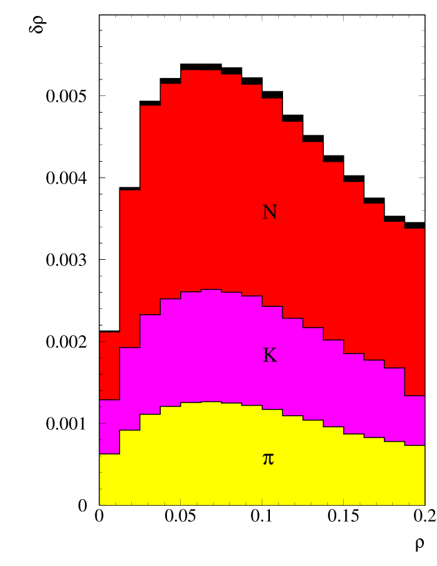
Figure 3: The contributions to $\delta\rho$, the difference between the mean jet mass $\rho$ in the default (massive) and $p$-scheme, coming from different hadron species ($\pi^{\pm}$, kaons and nucleons), shown as a function of $\rho$ in the default scheme.

While the necessary experimental corrections make it difficult to measure the difference between the schemes from data, the experiments’ reliance on simulation allows us to correct the existing data to any desired scheme without introducing significant additional systematic errors. We shall use Ariadne [26] to transform existing data [36, 19, 21] to a desired scheme whenever corresponding measurements in this scheme do not exist. Currently data exists for non-standard schemes only from DELPHI [21], H1 and ZEUS [22].

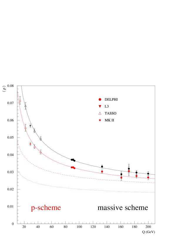
Figure 4: The jet mass $\rho$ as measured in the default scheme (upper set of points) and corrected to the $p$-scheme (lower set of points). The upper curve corresponds to a fit to the default-scheme points, while the lower three curves correspond to a fit to the $p$-scheme points (the dotted curve is the pure $\alpha_{\mathrm{s}}$ component, the dashed curve includes the ${\cal O}\left(\alpha_{\mathrm{s}}^{2}\right)$ term while the solid curve includes a power correction of the form eq. (3.7)).

In figure 4 we show data for the jet mass $\rho$ as function of $Q$ in the default and in the $p$-schemes. As $\rho$ is usually not given by the experiments, it was taken as the average of the measured heavy and light-jet masses. The lines in figure 4 correspond to fits using the ${\cal O}\left(\alpha_{\mathrm{s}}^{2}\right)$ perturbative prediction and a power correction of the form eq. (3.7).

The difference between the two middle (red solid and dashed) curves corresponds to the normal, ‘universal’, power correction. The difference between the upper two (red and black solid) curves is the mass-dependent power correction. One sees that above $Q=M_{Z}$ it is as large as the traditional $1/Q$ term, and it can be as much as $10\%$ of the mean value of the observable (cf. also table 3). For a general observables differences between the $p$ and $E$-schemes at $Q=M_{Z}$ are of the order of a few percent, whereas differences between decay and $E$-schemes are between $5$ and $10\%$ of the observable.

So while none of our previous analysis has given us any indication of the absolute size of mass-induced effects, comparisons in this section have shown that the absolute size of mass effects at $Q=M_{Z}$ due to hadrons can be sizable portion of the non-perturbative power-corrections.

Further results of comparisons with data, transformed to various schemes, will be presented in section 6.

5.2 Comparison to predictions

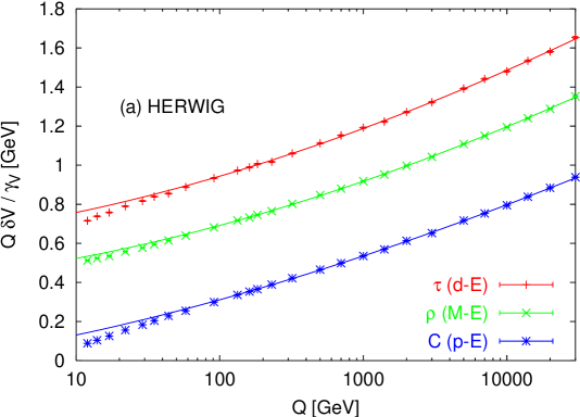
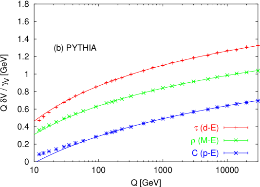
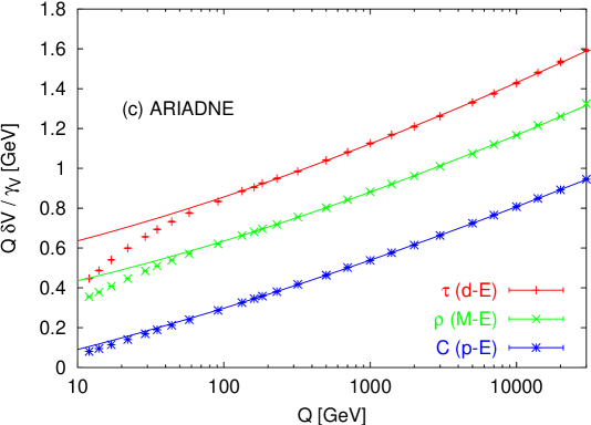
Figure 5: Herwig, Pythia and Ariadne results for the differences between pairs of measurement schemes for three observables. In all cases the differences have been normalised to $\gamma_{\cal V}$. The lines are fits of the form eq. (5.1) to the points with $Q>100\,\mbox{Ge\kern-0.86108ptV}$. These figures have been generated using events with primary down-quarks; the labels $(d-E)$, $(M-E)$ and $(p-E)$ indicate differences between the decay and E-schemes, the massive and $E$-schemes and the $p$ and $E$-schemes respectively.

Here we compare Monte Carlo results with the predictions of sections 3 and 4. There are two main predictions which we wish to test. Firstly that the leading energy-dependence of mass-dependent effects is $(\ln^{A}Q)/Q$; secondly that the coefficient of the leading energy dependence is proportional to $\gamma_{\cal V}$. We are also interested in examining a third, more qualitative prediction, namely that certain subsets of observables have similar subleading $1/Q$ mass effects.

We shall study results from three Monte Carlo event generators: Herwig [25], Pythia [27] and Ariadne [26]. Let us first illustrate the kind of behaviour that is seen by examining three observables: the difference between the $p$ (default) and $E$-schemes for the $C$-parameter, the difference between the massive (default) and $E$-schemes for the jet mass and the difference between the decay and $E$-schemes for the thrust. These differences (multiplied by $Q$) are shown as a function of $Q$ in figures 5a, 5b and 5c for Herwig and Pythia and Ariadne respectively. They have all been normalised to the appropriate $\gamma_{\cal V}$.

Pure $\gamma_{\cal V}/Q$ corrections would lead to superimposed flat lines. The fact that the lines rise for all three event generators is consistent with the fact that we have a correction enhanced at larger values of $Q$. But the nature of the $Q$ dependence is not consistent between the different programs. For Herwig and Ariadne the second derivative is positive and roughly consistent with $\ln^{A}Q$ with $A\simeq 1.6$ as predicted in eq. (4.26). On the other hand the Pythia results are inconsistent with such a hypothesis — we return to this problem shortly.

Our second prediction in eq. (4.26) was that the $Q$-dependence should be proportional to $\gamma_{\cal V}$ — the fact that our observables (normalised to $\gamma_{\cal V}$) have very similar $Q$ dependences supports this hypothesis. This is true for all three event generators.

To study these questions more systematically we fit a formula of the following form

$$\langle\delta_{m}{\cal V}\rangle=\frac{\gamma_{\cal V}}{Q}\left(\epsilon\ln^{A_{\mathrm{eff}}}\frac{Q}{\Lambda}\,+\,B\right)\,,$$ (5.1)

to $\langle\delta_{m}{\cal V}(Q)\rangle$, where $\epsilon$, $A_{\mathrm{eff}}$ and $B$ are the fit parameters (we take $\Lambda=0.2\,\mbox{Ge\kern-0.86108ptV}$). Implicit in this procedure is the assumption that terms with subleading energy dependence are reasonably well approximated by $\gamma_{\cal V}B/Q$ (fits involving more sophisticated forms for the subleading terms turn out to be fairly unstable). To reduce the impact of subleading effects we only fit points with $Q>100\,\mbox{Ge\kern-0.86108ptV}$. We have generated $10^{5}$ events per point.

We expect $A_{\mathrm{eff}}$ to be somewhere between the $n_{\mathrm{f}}=5$ and $n_{\mathrm{f}}=6$ values of $A=1.565$ and $A=1.714$. The results for $A_{\mathrm{eff}}$ are shown in the left hand plot of figure 6, for all three event generators, together with bands representing the predicted $n_{\mathrm{f}}=5$ and $n_{\mathrm{f}}=6$ values for $A$. Almost all the Pythia results have $A_{\mathrm{eff}}\simeq 0$ which is a signal of a dependence of the form $\ln\ln Q/\Lambda$. The Herwig and Ariadne results in general lie close to the predicted value for $A$. Most of the observables lie to within $\pm 0.1$ of the expected range, the notable exceptions being the difference between the decay and $E$-schemes for the heavy-jet mass and the broadenings. The broadenings in the decay scheme are quite delicate observables because they involve an expansion in powers of $\sqrt{\alpha_{\mathrm{s}}}$ which may be quite slowly convergent. In the case of the heavy-jet mass it is not too clear what is going wrong though it may well be related to the non-inclusiveness of the variable (cf. appendix D).

It is of interest to establish whether the inconsistency between our prediction and Pythia is due to the nature of the hadronisation or to the parton showering. If it were the former we might think that we had been too naive in assuming LPHD and an absence of qualitative changes due to hadronisation. Two distinct arguments support the hypothesis that the problem lies with the parton showering. One is that Ariadne uses the same string fragmentation routines as Pythia and so the problem must lie in the part of the physics which is treated differently between the two programs (the parton showering). The second argument comes from a direct investigation of the Pythia parton level: in Pythia, parton level gluons are massless so we cannot simply look at the difference between two mass-schemes. However mass effects are just related to the sum of the inverse energies of all the particles, so we can instead look directly at the behaviour of $D_{-1}(Y=\ln Q/\Lambda)$ (cf. eq. (4.4)) at both parton and hadron level (where it is best examined for individual hadron species) and check that it has the right energy dependence. We find that in Pythia both at parton and hadron levels, $D_{-1}(Y)$ rises too slowly with energy, while Herwig for example shows an energy dependence which is consistent with our prediction, both at parton and hadron level. This suggests that the parton showering present in Pythia might be lacking some of the dynamics associated with the coherent branching approach used in section 4.

Problems with coherence should have implications also for hadron multiplicities. If we restrict ourselves to ‘uds’ primary-quark events, we find that the ratio of Herwig and Ariadne $\pi^{\pm}$ multiplicities is essentially independent of $Q$ (to within $1\%$ for $Q$ between $100\,\mbox{Ge\kern-0.86108ptV}$ and $30\,\mbox{Te\kern-0.86108ptV}$). The ratio of Pythia to Ariadne $\pi^{\pm}$ multiplicities on the other hand decreases by about $13\%$ over this range. We note in passing that the $\pi^{\pm}$ multiplicities from Herwig and Ariadne at any given $Q$ differ by about $8\%$, and that if one includes heavy primary quarks the situation is more complicated.

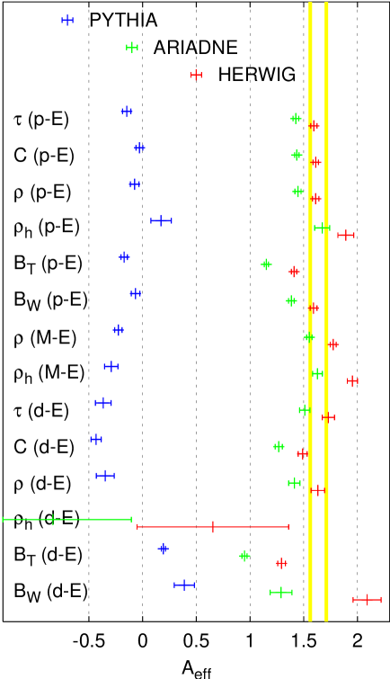
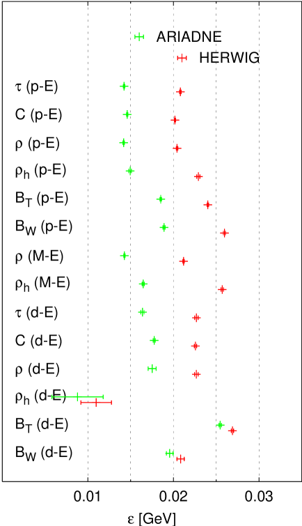
Figure 6: The left-hand plot shows the power $A_{\mathrm{eff}}$ ‘measured’ for a range of observables from Pythia, Ariadne and Herwig; the yellow bands are the expected values for $n_{\mathrm{f}}=5$ and $n_{\mathrm{f}}=6$. With $A_{\mathrm{eff}}$ fixed to its predicted $n_{\mathrm{f}}=5$ value, the values of $\epsilon$ fitted for the different observables are shown in the right-hand plot (just Ariadne and Herwig). The fits are carried out for $Q>100\,\mbox{Ge\kern-0.86108ptV}$ to reduce their sensitivity to subleading effects using only events with $d$ primary quarks. Errors are statistical from $10^{5}$ events at each of 17 energies.

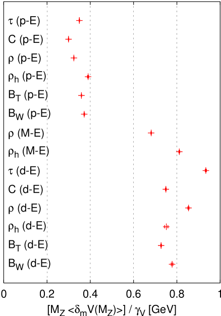
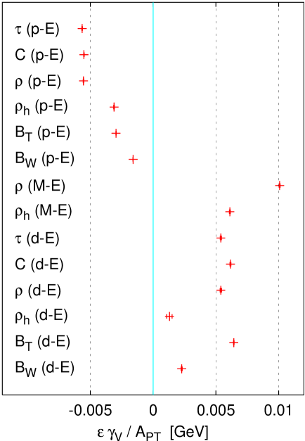
Figure 7: The left hand plot shows the value of the observables at a fixed value of $Q=M_{Z}$, normalised to $\gamma_{\cal V}$. The right hand plot shows the $Q$-dependence of the various observables normalised to the leading-order perturbative coefficient rather than to $\gamma_{\cal V}$. Results are shown for Herwig only.

Our second prediction was that the leading $Q$-dependence should be proportional to $\gamma_{\cal V}$. To test this systematically we fix $A_{\mathrm{eff}}$ to be equal to $A=1.565$ and fit for the values of $\epsilon$ and $B$ in eq. (5.1) (using the same range of $Q$ as before). We do this only for Herwig and Ariadne. The results are shown in the right hand plot of fig. 6. The mean value of $\epsilon$ is about $0.023\,\mbox{Ge\kern-0.86108ptV}$ for Herwig and about $0.016\,\mbox{Ge\kern-0.86108ptV}$ for Ariadne. One should not be misled into thinking that these small numbers imply small effects — they get multiplied by $\ln^{A}Q/\Lambda$, which is about $17$ for $Q=M_{Z}$! The range of $\epsilon$ values for different observables is typically about $\pm 10\%$ from the central value (with the exception of the difference between the decay and $E$-schemes for $\rho_{h}$). Thus our two main predictions, concerning the energy dependence and the relative normalisation of mass-dependent effects are in remarkable agreement with Monte Carlo results.

We can also examine the mass correction at a given fixed value of $Q$, rather than its $Q$-dependence. In the left-hand plot of figure 7 we show $Q\langle\delta_{m}{\cal V}(Q)\rangle/\gamma_{\cal V}$ for $Q=M_{Z}$. The points seem to fall into two groups: those corresponding to differences between the $p$ and $E$-schemes, and those corresponding to differences between the massive and $E$-schemes (jet masses) and the decay and $E$ schemes. The differences between and $p$ and $E$-schemes are all governed by the functions $\delta c_{\cal V}$ in figure 2 which have a maximum: these functions have very similar shapes, meaning that whatever the form of $\Phi_{h}(k_{t},Y)$ in (4.16) the integral will be proportional to $\gamma_{\cal V}$. This statement was made earlier in the form of eq. (3.20). The fact that the points for the jet masses (massive minus $E$-schemes) and the decay minus $E$-schemes are higher was anticipated in eq. (3.21), since after accounting for the rescaling by $\gamma_{\cal V}$, their $\delta c_{\cal V}$’s remain larger than those of the other variables.

Finally, for entertainment purposes, in the right hand plot of figure 7 we show the $Q$-dependence normalised not to $\gamma_{\cal V}$ but to $A_{PT}$, the first coefficient of the perturbative expansion of the event shape. It illustrates the fact that mass effects vary significantly in size and sign from one observable to the next — and that the ability to predict that pattern of this variation is a non-trivial achievement!

5.3 Resonance and hadron-level decay scheme results

In section 3.4 we mentioned that a phenomenological advantage of the decay scheme is that regardless of the hadronic level from which we start the decay scheme results are very similar. To verify this we start with two hadronic levels: a normal hadronic level, as defined earlier and a resonance level which is ‘defined’ as the first level of hadrons produced in Pythia or Ariadne. We then look at the difference between decay-scheme event-shape values for these two hadronic levels compared to the difference between the $E$-scheme values. Results obtained from Ariadne are given (in $\%$) in table 4: they show that for most variables, in the decay scheme one is very insensitive to the initial hadronic level. This is not completely trivial since the actual decays that take one from resonance to hadron level are not just the artificial massless two-body decays of the decay scheme.

${\cal V}$	$\tau$	$\rho$	$\rho_{h}$	$C$	$B_{T}$	$B_{W}$
$\frac{{\cal V}_{\mathrm{decay},\mathrm{had}}-{\cal V}_{\mathrm{decay},\mathrm{res}}}{{\cal V}_{E,\mathrm{had}}-{\cal V}_{E,\mathrm{res}}}(\%)$	$1.1\pm 0.2$	$-7.3\pm 0.9$	$0.8\pm 0.2$	$1.9\pm 0.1$	$1.5\pm 0.2$	$-1.5\pm 0.5$

Table 4: Percentage dependence of decay scheme results on the choice of the initial hadronic level (‘normal hadron’ or resonance level), relative to the dependence of $E$-scheme results on the hadronic level. The numbers are shown for $Q=M_{Z}$ using results from Ariadne.

For most of the variables the ratio shown in table 4 scales roughly as $1/Q$, i.e. at these energies the difference between decay schemes for the two hadronic levels is dominated by a $1/Q^{2}$ correction rather than a $1/Q$ correction. The jet mass $\rho$ and the wide-jet broadening seem to be more complex (note also the different sign of the correction compared to the other observables, and the somewhat larger value for $\rho$), but the origins of the differences have yet to be identified.

A point worth noting (we will see a related point in section 6) is that at lower energies, the good correspondence between the two decay-scheme results holds only if heavy-quark decays are taken into account separately.

5.4 Total hadronisation

So far in this section we have examined differences between various measurement schemes and various hadronic levels. We observed in section 4.3 that, since the difference between any two hadronic levels contains terms proportional to $(\ln Q)^{A}/Q$, the total hadronisation corrections in going to an arbitrary hadronic level must also contain such terms. Additionally, hadronisation itself might introduce a contribution proportional $(\ln Q)^{A}/Q$, as a consequence of the reshuffling of momenta associated with the production of massive hadrons. We introduced the parameter $\mu_{\ell}$ to represent the normalisation of such a component for a given hadronic level $\ell$, and pointed out that it could quite conceivably be negative, for example if the energy required to produce the hadron masses comes partially from transverse degrees of freedom.

One may wonder what happens in the hadronisation models used in Monte Carlo event generators. The various curves in figure 8 show the corrections to $\tau$ (multiplied by $Q$) in going from parton level to each of a variety of hadronic levels, as determined from Ariadne. The first level after hadronisation is the resonance level — the fact the corresponding line has negative slope means that $\mu_{\ell}$ is negative. Indeed the hadronisation corrections change sign at around $200\,\mbox{Ge\kern-0.86108ptV}$!

Figure 8: The difference between hadron and parton level results for $\tau$ (multiplied by $Q$), shown as a function of $Q$. Curves are shown for three different hadronic levels, and have been obtained from the Ariadne event generator with only light primary quarks. The thrust is defined in the $E$-scheme.

However we expected mass effects to have a characteristic signature, namely to contain a term $(\ln Q)^{A}/Q$ with $A\simeq 1.6$. If we carry out a fit (analogous to those carried out in section 5.2) to determine the effective power for the resonance level curve then we obtain $A_{\mathrm{eff}}\simeq 1.0$. This could be due to subleading mass effects, or some completely different effect which has yet to be considered.

At other hadronic levels one sees a weaker $Q$ dependence — the positive $(\ln Q)^{A}/Q$ contribution from hadron decays cancels a large part of the negative contribution from the hadronisation. This in itself is an interesting, and even quite natural, result: the negative contribution from hadronisation is of the same order as the positive contribution from the decay of all hadrons!

Of course these observations may be very specific to the hadronisation model being considered. It would have been interesting to carry out a similar exercise with the Herwig event generator, however there the situation is more complex because the gluons have a (large) mass ($0.8\,\mbox{Ge\kern-0.86108ptV}$). So in some sense, part of the hadronisation mass effects will already be implicitly included in the parton showering and a straightforward investigation of the difference between hadron and parton levels will show up only a part of the mass effects (and there will be a large ambiguity coming from the choice of scheme in which to measure the parton level).

6 Fits to data

6.1 2-parameter fits

Following the suggestion of [3] it has become standard procedure in recent years to carry out simultaneous fits for $\alpha_{\mathrm{s}}$ and $\alpha_{0}$, with formulae of the form

$$\langle{\cal V}\rangle=C_{1}\frac{\alpha_{\mathrm{s}}}{2\pi}+C_{2}\frac{\alpha_{\mathrm{s}}^{2}}{(2\pi)^{2}}+c_{\cal V}\frac{a_{0}}{Q}\,,$$ (6.1)

where the $C_{i}$ are the perturbative coefficients for the mean value and $a_{0}$ is defined in terms of $\alpha_{0}$ and $\alpha_{\mathrm{s}}$ in eq. (3.7). In order to set the scene we show in figure 9a one-$\sigma$ confidence-level contours from such fits to data [36, 19, 21] for a range of event-shape variables, all in the default schemes. In the absence of mass effects the universality hypothesis states that the values of $\alpha_{\mathrm{s}}$ and $\alpha_{0}$ should be consistent for the different variables.

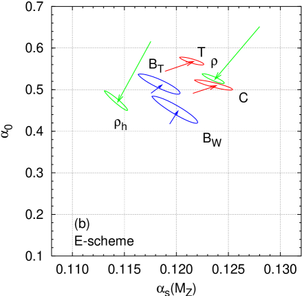
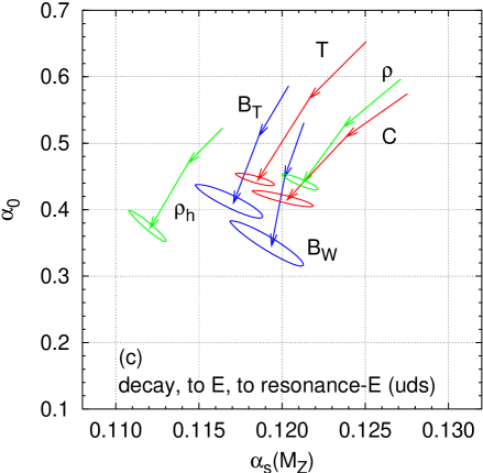
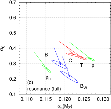
Figure 9: 1-$\sigma$ confidence-level contours from fits to event-shape variables in a range of schemes. (a) fits in the default schemes (normal hadron level); (b) fits in the $E$-scheme (normal hadron level), with arrows indicating the motion of the contour in going from the default to the $E$-scheme; (c) fits in the $E$-scheme at resonance level, with arrows indicating the motion of the contour from the decay-scheme, to the hadron-level $E$-scheme, to the resonance $E$-scheme — here the correction to resonance level has carried out using only events with light primary quarks; (d) fits in the $E$-scheme at resonance level where the correction to resonance level now includes events with heavy primary quarks as well — the arrows indicate the motion from the ‘uds’ resonance level.

Compared to the figures of this kind that one usually sees, one difference is the inclusion of a result for $\rho$ — until now generally only $\rho_{h}$ has been studied. While data do not exist for $\rho$ itself, there are some data on the light-jet mass $\rho_{l}$, and from this one can calculate $\rho=(\rho_{h}+\rho_{l})/2$. What one sees is a significant inconsistency between this variable and the others.

Of course we know that we should really be carrying out the fits with additional terms of the form (4.28), so as to take into account mass-dependent corrections. Let us for the time ignore $\mu_{\ell}$ (i.e. pretend it is conveniently zero!) and concentrate on the term involving $\gamma_{{\cal V}_{S}}\epsilon_{\ell}$ — this piece is measurement scheme-dependent. In the default schemes $\gamma_{{\cal V}_{S}}$ is positive for the jet masses, and negative for all the other variables (cf. table 2). If we ignore it then our fit parameters for $\rho$ and $\rho_{h}$ should come out larger than for the other variables. This is exactly what we see in figure 9a.

So if we want to be check universality we first have to ensure that these non-universal mass effect are absent, i.e. choose a scheme in which the $\gamma_{{\cal V}_{S}}$ are zero, namely the $E$-scheme (we could also use a scheme in which all the $\gamma_{\cal V}$ are more or less proportional to $c_{\cal V}$, such as the $p$-scheme). Accordingly in figure 9b we repeat the fits for $\alpha_{\mathrm{s}}$ and $\alpha_{0}$ but using $E$-scheme data. The arrows show how the best fit values have moved in going from the default to the $E$-schemes.

The switch to the $E$-scheme decreases the values of the jet masses, while it increases, by somewhat less (in accord with the opposite sign and smaller value of $\gamma_{\cal V}/c_{\cal V}$), the values of the other variables. We see a change in both $\alpha_{\mathrm{s}}$ and $\alpha_{0}$ because it is only through a linear combination of the $\alpha_{\mathrm{s}}$ and $\alpha_{0}$ $Q$-dependences that the fits can mimic a term of order $(\ln^{A}Q)/Q$. The ‘angle’ of the arrows depends on the relative amounts of $(\ln^{A}Q)/Q$ and plain $1/Q$ in the mass-correction: if mass effects involved just $1/Q$ corrections then only $\alpha_{0}$ would change. For the broadenings the situation is more complex because the ‘universal’ power correction goes as $1/(\sqrt{\alpha_{\mathrm{s}}}Q)$ which is more similar to a mass effect than a pure $1/Q$ term, so there is less need for a change in $\alpha_{\mathrm{s}}$ to mimic the mass effect.

In the $E$-scheme the universality picture changes with respect to the default schemes: whereas in the default scheme $\rho$ was clearly inconsistent with the other variables, in the $E$-scheme it is now very close to the thrust and the $C$-parameter. The heavy-jet mass on the other hand now seems to be the least consistent of the different variables as can be verified by examining the $\chi^{2}$ contribution from $\rho_{h}$ in a simultaneous fit to all variables. It may well be that the non-inclusiveness of this variable is responsible for its different behaviour, as is discussed in appendix D.

Now that we are in a scheme in which non-universal mass corrections have been eliminated we can turn our attention to the question of universal mass corrections, i.e. the contribution related to $\mu_{\ell}$ in eq. (4.28). A first question of interest is whether we actually need to worry about this term at all — maybe it is sufficiently small that it can be ignored altogether. We know that $\mu_{\ell}$ depends on the hadronisation level $\ell$. To gauge the importance of $\mu_{\ell}$ we study three levels, each in the $E$-scheme: the decay level (actually the decay scheme of the usual hadron level), the usual hadron level and a ‘resonance’ level. The latter is taken (arbitrarily) to consist of the first level hadrons produced in the Pythia/Ariadne string hadronisation routines. The results of 2-parameter fits to these different hadronic levels are shown in figure 9c: the arrows start from the decay level best fit, go to the usual hadron level best fit, and then to the resonance level, for which we also show the $1$-$\sigma$ contours.

All variables move more or less in the same direction and by the same amount — this is consistent with our knowledge that $\mu_{\ell}$ is multiplied by $c_{\cal V}$ (the broadenings are more complex and move a bit differently). Accordingly the situation regarding universality is essentially unchanged (if anything, in the resonance level it is somewhat improved). However in going from the decay to the resonance scheme $\alpha_{\mathrm{s}}$ changes by up to $0.007$; $\alpha_{0}$ is also sensitive to the hadronic level chosen and varies by up to $0.2$. At $Q=M_{Z}$ the variation in the observables themselves is of the order of $10$ to $15\%$. In other words mass effects, even in a ‘universal’ scheme, are responsible for a significant part of an observable’s value and have a non-trivial effect on fits for $\alpha_{\mathrm{s}}$ and $\alpha_{0}$.

If we had examined the same three hadronic levels in the $p$-scheme we would have seen even larger dependence on the scheme because of the contribution from the $\gamma_{{\cal V}_{p}}\epsilon_{\ell}$ term (recall that $\epsilon_{\ell}$, which is zero in the decay level, increases as one goes towards the resonance level, cf. eq. (4.30)). In particular the dependence of $\alpha_{\mathrm{s}}$ on the hadronic level should double, a consequence of the relation $\gamma_{{\cal V}_{p}}\simeq-\gamma_{{\cal V}_{\mathrm{decay}}}$. The complete range of values for $\alpha_{\mathrm{s}}$ and $\alpha_{0}$ in the different hadronic levels and $E$ and $p$ schemes is summarised for our different event-shape variables in figure 10.

​

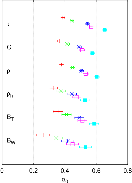
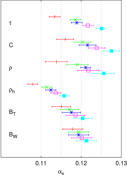
Figure 10: Plots showing $\alpha_{\mathrm{s}}$ and $\alpha_{0}$ values obtained by fitting to data corrected to a variety of schemes and hadronisation levels. Corrections relative to the default schemes have been obtained using Ariadne, as discussed in the text.

Coming back to figure 9c, one important point which we have yet to mention is that the corrections from normal hadron to the resonance level have been calculated using events with only light (uds) primary quarks. The corrections have then been applied to all events (including those with heavy primary quarks). This is equivalent to reconstructing all resonances except those associated with primary heavy quarks. The reason for doing this is that in an event with heavy primary quarks, going to the resonance level involves a reconstruction of the heavy-quark hadrons. In the usual hadron level these have decayed and the invariant mass $m_{q}$ of the hadron contributes to the event shape at the level $m_{q}^{2}/Q^{2}$ (for a more detailed discussion, see appendix C, and also the discussion of heavy-quark decays in the context of fragmentation functions in [37]), whereas in the resonance level ($E$ or $p$) schemes the mass of a forward moving hadron has little impact on the value of the observable (other than at order $\alpha_{\mathrm{s}}m_{q}^{2}/Q^{2}$). If we had shown figure 9c including heavy-quark events to carry out the correction from hadron to resonance level, the combination of the heavy-quark decay effect and the usual light-hadron mass effects would have made it difficult to interpret the figure. This is the reason why we applied a correction calculated using only events with light primary quarks.

In order to give the ‘full story’, in figure 9d we show the $1$-$\sigma$ contours which come from including primary heavy quarks in our correction to resonance level (the arrows come from the ‘uds’ resonance level). The arrows are roughly at right angles to those in the other plots — this is closely linked to the fact the difference between the ‘uds’ and full resonance levels is a $1/Q^{2}$ correction (i.e. something which dies off faster than $1/Q$, so that we need the difference between a $1/Q$ and an $\alpha_{\mathrm{s}}(Q)$ term in order to approximate it over the given energy range). Despite their significant effect on the best fit for $\alpha_{\mathrm{s}}$, the heavy-quark decay changes the value of the observables significantly only at low $Q$ values. At $M_{Z}$ for example the effect on the thrust is $2\%$ (compared to $16\%$ from the decay of all the light-resonances).

A final point worth mentioning is the following: if one believes, as implied by Ariadne in figure 8, that of the various hadronic levels the decay-level is that with the smallest contamination from mass effects, then choosing this hadronic level for a fit to $\alpha_{\mathrm{s}}$ and $\alpha_{0}$, and accounting also for heavy-quark decays (by either reconstructing the heavy-quark hadron, or explicitly including the contribution from heavy-quark decay as calculated in appendix C) will lead us to high results for $\alpha_{\mathrm{s}}$, around $0.130$. This means that there may well be room for the large higher-order perturbative coefficients predicted by Gardi and Grunberg in [16], which for normal $p$-scheme measurements imply a value for $\alpha_{\mathrm{s}}$ of about $0.110$.

6.2 3-parameter fits

${\cal V}$	$\alpha_{\mathrm{s}}$	$\alpha_{0}$	$\mu_{\ell}$	$\chi^{2}/$d.o.f.
$\tau$ res. (uds)	$0.1448\pm 0.0141$	$0.891\pm 0.237$	$-0.077\pm 0.042$	$56.2/44$
$\tau$ res. (full)	$0.1206\pm 0.0095$	$0.262\pm 0.161$	$\hskip 3.33333pt0.012\pm 0.027$	$57.7/44$

Table 5: Results from a 3-parameter fit to the thrust in two different hadronic levels (‘uds’ and full resonance levels, $E$-scheme).

That fact that the event-shape values depend significantly on the particular hadronic level chosen implies an important contribution to the event-shape value from a term proportional to $\mu_{\ell}$. This means that we should really be fitting for $\mu_{\ell}$ as well as for $\alpha_{\mathrm{s}}$ and $\alpha_{0}$, using an equation of the form

$$\langle{\cal V}\rangle=C_{1}\frac{\alpha_{\mathrm{s}}}{2\pi}+C_{2}\frac{\alpha_{\mathrm{s}}^{2}}{(2\pi)^{2}}+c_{\cal V}\frac{a_{0}}{Q}+c_{\cal V}\frac{\mu_{\ell}}{Q}\ln^{A}\frac{Q}{\Lambda}\,.$$ (6.2)

In the last term we fix $\Lambda=0.2\,\mbox{Ge\kern-0.86108ptV}$ (tying $\Lambda$ to the value of $\alpha_{\mathrm{s}}(M_{Z})$, in practice the replacement of $\ln\frac{Q}{\Lambda}$ by $2\pi/(\beta_{0}\alpha_{\mathrm{s}})$, makes little difference). It turns out that the inclusion of the last term makes the fitting procedure quite unstable, and leads to large (correlated) errors on the individual fit parameters as well as a strong dependence on subleading effects. Consequently the significance of the results is limited.

To illustrate the point, we consider the thrust at two hadronic levels (both in the $E$-scheme): the ‘uds’ resonance level and the ‘full’ resonance level. The former is subject to the $m_{b}^{2}/Q^{2}$ corrections arising from heavy quark decay, whereas the latter should be free of them (but will still have other $1/Q^{2}$ corrections). The fit results in the two cases, table 5, give completely different pictures. In the ‘uds’ resonance level, the fit results seem inconsistent with our expectations for $\alpha_{\mathrm{s}}$ (if only at $2$-$\sigma$). In the full resonance level the value for $\alpha_{\mathrm{s}}$ is ‘as we would like’, but the $\chi^{2}$ is a bit larger.

There may of course be other subleading effects that we have not yet considered (for example higher-order perturbative corrections) which could cause further big changes. Additionally the event generator used to correct to a given scheme may not have the right behaviour at low values of $Q$. So the systematics are such that, at least currently, it is difficult to extract reliable information from a $3$-parameter fit: the uncertainties on $\alpha_{\mathrm{s}}$ are even larger than those which arise by considering a range of hadronic levels in a 2-parameter $\alpha_{\mathrm{s}},\alpha_{0}$ fit and $\mu_{\ell}$ remains unconstrained.

If our main aim is to determine $\mu_{\ell}$ then we can try a 2-parameter fit with $\alpha_{\mathrm{s}}$ fixed. But here again we find that the systematic uncertainties on $\mu_{\ell}$, are of the same order as the parameter expected size of the parameter itself, i.e. about $0.02$ (cf. the values of $\epsilon$ in figure 6).

7 Conclusions

The Good.

In this paper we have understood many features of the contributions to event-shapes that are associated with hadron masses: there are two classes of contribution, both of which scale as $(\ln Q)^{A}/Q$. The contribution from the ‘non-universal class’ depends on the details of whether the variable is defined in terms of $3$-momenta, energies and angles, or a mixture of the two, and we can calculate the relative magnitude of the mass-correction for different definition schemes. It turns out that there is a privileged scheme ($E$-scheme) in which non-universal mass corrections are absent, because their coefficient is zero. The ‘universal’ class of mass corrections gives contributions proportional to the same coefficient $c_{\cal V}$ that appears in calculations of traditional universal (massless) $1/Q$ corrections; universal mass corrections are present regardless of the definition of the event-shape variable, and they are proportional to a new non-perturbative parameter $\mu_{\ell}$ which depends on the particular hadronic level $\ell$ (i.e. stage of the decay chain) at which we observe the event.

In traditional power correction analyses, $1/Q$ power corrections are often given a quasi-perturbative interpretation in terms of an infrared-finite coupling, reflecting the fact that they are associated with the strictly perturbative concept of the renormalon divergence of perturbation theory. The parameter $\alpha_{0}$ that appears in such analyses can be related to a moment of the coupling in the infrared. On the other hand our new parameter $\mu_{\ell}$ is more related to the ‘reshuffling’ of momenta associated with the production of mass — in this sense it is a much more intimately associated with the dynamics of hadronisation, and there is perhaps even a possibility that its determination could give us qualitative information about hadronisation. It is not currently clear whether perturbative contributions could also give contributions with a similar $Q$-dependence.

Our analytical predictions for differences between different measurement schemes agree well with results from two commonly used Monte Carlo event generators, Herwig and Ariadne. Furthermore, in fits for $\alpha_{\mathrm{s}}$ and $\alpha_{0}$ from a range of event-shape variables, they explain a pattern observed both in $e^{+}e^{-}$ and DIS of the jet masses giving significantly larger values of both $\alpha_{\mathrm{s}}$ and $\alpha_{0}$ than other variables: this is because in the default schemes there are positive (non-universal) mass-corrections for the jet masses and negative corrections for the other variables. Measuring all variables in the $E$-scheme leads to a significant improvement in the consistency between the jet masses and the other variables. We also note that for the jet masses the $p$ and $E$-schemes are relatively insensitive to certain experimental systematics (associated with difficulties in identifying hadrons) which are relevant in the default measurement scheme.

The Bad.

Unfortunately it seems that a direct experimental verification of the properties of mass effects is quite difficult. In principle mass effects can be seen by looking at the difference between two measurement schemes for the same variable (say massive and $E$-schemes in the case of the jet mass). However the experimental determination of such differences relies on the accurate identification of the mass of each particle in an event, whereas the experimental procedure usually just involves the assignment of the pion mass to each hadron. Since a large part of mass effects seems to come from kaons and nucleons this is a poor approximation. Given that the results are then corrected for what cannot be seen, using Monte Carlo programs, the resulting ‘measurement’ of the difference between two schemes is likely to be as much a reflection of the properties of the Monte Carlo events as of the actual events!

It so happens that in one of the Monte Carlo programs most commonly used for correcting data, Pythia, the $Q$-dependence of mass effects differs significantly from our predictions at very high energies, going very roughly as $(\ln\ln Q)/Q$ rather than $(\ln Q)^{A}/Q$. This is probably related to approximations in Pythia’s implementation of coherence. Fortunately for measurements in the $p$ or $E$-schemes this should not have too large an effect on the practical determination of event shape values since the 3-momentum or energy are close to what is truly measured by detectors (it is the difference between them that is poorly measured). Furthermore at today’s energies the discrepancy in the Pythia energy dependence is a small effect compared to other differences between event generators.

In general, given the difficulties of a direct measurement of mass effects in event shapes, for an experimental test of the picture outlined here it might be worth investigating the feasibility of measuring some other observable expected to depend on the same $(-1)^{\mathrm{th}}$ moment of particle energies. The simplest might be $\sum_{i}1/E_{i}$ where the sum runs over charged tracks. This might give an idea of whether the LPHD hypothesis used in this paper works also for negative moments, where it has so far never been tested.

One ‘negative’ implication of our results relates to the determination of the perturbative and non-perturbative parameters of QCD. We would like to measure our new non-perturbative parameter $\mu_{\ell}$. But the degeneracy in a 3-parameter fit for $\alpha_{\mathrm{s}}$, $\alpha_{0}$ and $\mu_{\ell}$ is such that the currently available data are not precise enough to give us any meaningful constraints on any of the fit parameters. Furthermore the fit results are very unstable with respect to systematic uncertainties. Given this limitation we might decide that for the time being we should carry on as before with two-parameter fits $\alpha_{\mathrm{s}}$ and $\alpha_{0}$ (of course with the event-shape variables now measured in the $E$-scheme). Our having neglected a parameter in the fit will translate to systematic errors on $\alpha_{\mathrm{s}}$ and $\alpha_{0}$. We can try to gauge the size of the systematics by carrying out the fit on results at different levels of the hadronic decay chain (using Monte Carlo results to determine the correction) — this suggests systematics of the order of $\pm 0.004$ on $\alpha_{\mathrm{s}}$ and of about $\pm 0.1$ on $\alpha_{0}$.

The Ugly.

In the course of our studies we have come across two effects, unrelated to light-hadron masses, that have a significant impact on event-shape studies and so warrant further investigation.

Firstly there is the observation that heavy-quark effects have a large impact on fit values for $\alpha_{\mathrm{s}}$ and $\alpha_{0}$ — measuring an event shape before and after heavy quark decay modifies $\alpha_{\mathrm{s}}$ values by up to $0.006$, even though at $M_{Z}$ the effect of heavy quark decay is only $2\%$. This peculiar behaviour is seen because the $m_{q}^{2}/Q^{2}$ contribution from quark decay is simulated by an increase of $\alpha_{\mathrm{s}}$ and a decrease of $\alpha_{0}$. Given that the tools for studying heavy-quark effects in event shapes are well-established, there is a strong argument for carrying out analyses that make full use of them.

Secondly fits for the heavy-jet mass (a very non-inclusive variable) lead to values for $\alpha_{\mathrm{s}}$ which are about $10\%$ smaller than for inclusive variables like the thrust or the mean jet mass. This needs to be understood. It could be due to a difference in the behaviour of the perturbation series at higher orders. But in appendix D there is evidence from Monte Carlo simulations that hadronisation corrections for $\rho_{h}$ have unusual characteristics: in contrast to what is seen in more inclusive variables, the hadronisation depends strongly on the underlying hard configuration. There is therefore a need to develop techniques allowing a more formal approach to the study of such problems.

Appendix A Summary of notation

For convenience we give here a summary of the definition of the various schemes introduced in this article.

$\boldsymbol{p}$-scheme

Scheme in which the observable is defined solely in terms of particle 3-momenta.

$\boldsymbol{E}$-scheme

Scheme in which the observable is defined solely in terms of particle energies and angles.

decay-scheme

Scheme in which all massive particles are decayed isotropically into pairs of massless particles. The observable is then calculated using the resulting ensemble of massless particles.

We also summarise some of the other notation used and introduced in this article.

$\boldsymbol{{\cal V}}$

An event-shape variable.

$\boldsymbol{{\cal V}_{p},{\cal V}_{E},{\cal V}_{\mathrm{decay}}}$

An event-shape variable in $p$, $E$ or decay-scheme, respectively.

$\boldsymbol{c_{\cal V}}$

The coefficient of the ‘traditional’ power correction for the observable ${\cal V}$, introduced in eq. (3.5) and given for a range of observables in table 1.

$\boldsymbol{\langle\delta_{m}{\cal V}\rangle}$

The non-universal mass-dependent correction to the mean value of the observable ${\cal V}$, cf. eq. (3.10).

$\boldsymbol{\delta c_{\cal V}(m^{2}/k_{t}^{2})}$

The modification to $c_{\cal V}$ for a particle with a given $m^{2}/k_{t}^{2}$, cf. eq. (3.12).

$\boldsymbol{\gamma_{\cal V}}$

The coefficient of the leading $m^{2}/k_{t}^{2}$ dependence of $\delta c_{\cal V}(m^{2}/k_{t}^{2})$ for $k_{t}\gg m$, as defined in eq. (3.18). It is shown for a range of variables in their default schemes in table 2.

$\boldsymbol{X_{\mathrm{decay}}(m^{2}/k_{t}^{2})}$

The mean relative change in the sum of $|k_{t}|$’s due to the decay of a massive particle of mass $m^{2}$ and transverse momentum $k_{t}^{2}$, as defined in eq. (3.28).

$\boldsymbol{A}$

Shorthand for $4C_{\mathrm{A}}/\beta_{0}$. Mass-dependent corrections have a leading term proportional to $(\ln Q/\Lambda)^{A}/Q$.

$\boldsymbol{\epsilon_{\ell}}$

The normalisation of the non-universal mass-dependent correction for a hadronic level $\ell$, cf. eqs. (4.27, 4.28).

$\boldsymbol{\mu_{\ell}}$

The normalisation of the universal mass-dependent correction for a hadronic level $\ell$, cf. eqs. (4.28, 4.29).

Appendix B Broadenings in the decay scheme

In determining the QCD-based predictions for mass-effects in section 4.2 we made the assumption that for all variables considered, mass effects matter only in the region of small rapidities. As a result we could ignore the rapidity dependence of the hadron distribution, because it is significant only at large rapidities. More precisely we expanded the rapidity dependence of $\Phi_{h,-\omega}(\eta,Y)$ and showed that it gave terms suppressed by a power of $\alpha_{\mathrm{s}}$,

$$\int d\eta\;\delta f_{{\cal V},\omega}(\eta)\;\alpha_{\mathrm{s}}\eta={\cal O}\left(\alpha_{\mathrm{s}}\right),$$ (B.1)

which holds if $\delta f_{{\cal V},\omega}(\eta)$ decreases sufficiently rapidly with $\eta$. This works for all variables except the broadenings in the decay scheme, the reason being that for the broadenings the difference between the normal and decay schemes is sensitive to particle masses for particles up to rapidities of order $1/\sqrt{\alpha_{\mathrm{s}}}$. For the example the total jet broadening has

$$\delta f_{B_{T,\mathrm{decay}},\omega}(\eta)=f_{B_{T}}(\eta)\,X_{\mathrm{decay},\omega}$$ (B.2)

where we can write [15]

$$f_{B_{T}}(\eta)\simeq\int_{0}^{\infty}d\ell\,\Theta\left(\ell+\eta_{0}-\eta\right)\Theta(\eta)\;\left(\frac{2\alpha_{\mathrm{s}}C_{\mathrm{F}}\ell}{\pi}+\frac{C_{\mathrm{F}}\alpha_{\mathrm{s}}^{2}\beta_{0}\ell^{2}}{(\pi)^{2}}\right)e^{-\frac{\alpha_{\mathrm{s}}C_{\mathrm{F}}\ell^{2}}{\pi}-\frac{C_{\mathrm{F}}\beta_{0}\alpha_{\mathrm{s}}^{2}\ell^{3}}{3\pi^{2}}}\,.$$ (B.3)

(We recall that here $\eta_{0}$ has been defined with an additional $3/4$ compared to what is given in [15]). Since $f_{B_{T}}$ is roughly $1$ up to $\eta\sim 1/\sqrt{\alpha_{\mathrm{s}}}$ the integral (B.1) is of order $1$ (while the leading term is of order $1/\sqrt{\alpha_{\mathrm{s}}}$, cf. table 1). Even though this term is subleading, in analogy with what is done for the $c_{\cal V}$’s, we wish to control it, which can be achieved as follows. First we write

$$\int d\eta\,\,\delta f_{{\cal V},\omega}(\eta)\,\Phi_{h,-\omega}(\eta,Y)=\Phi_{h,-\omega}(0,Y)\delta c_{{\cal V},\omega}$$ (B.4)

where the $\eta$ dependence of $\Phi_{h,-\omega}$ has been absorbed into $\delta c_{{\cal V},\omega}$:

$$\delta c_{{\cal V},\omega}=\int d\eta\;\delta f_{{\cal V}_{\mathrm{decay}},\omega}(\eta)\left(1-\frac{A}{\omega}\frac{\eta}{Y}+\cdots\right)\,.$$ (B.5)

Substituting in the above equations for $\delta f_{B_{T,\mathrm{decay}},\omega}$ gives

$$\delta c_{B_{T,\mathrm{decay}},\omega}=\left(\frac{\pi}{2\sqrt{C_{\mathrm{F}}\alpha_{\mathrm{s}}}}-\frac{\beta_{0}}{6C_{\mathrm{F}}}+\eta_{0}-\frac{A}{\omega}\frac{\beta_{0}}{4C_{\mathrm{F}}}\right)X_{\mathrm{decay},\omega}\,.$$ (B.6)

In section 3.4 we had stated that

$$\delta c_{{\cal V}_{\mathrm{decay}},\omega}=c_{\cal V}\,X_{\mathrm{decay},\omega}\,.$$

If we compare our result (B.6) with $c_{B_{T}}$ in table 1, we find that there is an additional term $-\frac{A\beta_{0}}{4C_{\mathrm{F}}\omega}=-\frac{C_{\mathrm{A}}}{C_{\mathrm{F}}\omega}$, not present in $c_{\cal V}$. This is the piece which arises from the rapidity dependence of the hadron distribution and in practice it gives quite a large correction to $\delta c_{B_{T,\mathrm{decay}},\omega}$.

The corresponding derivation for the wide-jet broadening involves the use of

$$\delta f_{B_{W,\mathrm{decay}},\omega}(\eta)=f_{B_{W}}(\eta)\,X_{\mathrm{decay},\omega}\,,$$ (B.7)

where

$$f_{B_{W}}(\eta)\simeq\frac{1}{2}\int_{0}^{\infty}d\ell\,\Theta\left(\ell+\eta_{0}-\eta\right)\Theta(\eta)\;\left(\frac{4\alpha_{\mathrm{s}}C_{\mathrm{F}}\ell}{\pi}+\frac{2C_{\mathrm{F}}\alpha_{\mathrm{s}}^{2}\beta_{0}\ell^{2}}{(\pi)^{2}}\right)e^{-\frac{2\alpha_{\mathrm{s}}C_{\mathrm{F}}\ell^{2}}{\pi}-\frac{2C_{\mathrm{F}}\beta_{0}\alpha_{\mathrm{s}}^{2}\ell^{3}}{3\pi^{2}}}\,.$$ (B.8)

We thus obtain

$$\delta c_{B_{W,\mathrm{decay}},\omega}=X_{\mathrm{decay},\omega}\left(\frac{\pi}{4\sqrt{2C_{\mathrm{F}}\alpha_{\mathrm{s}}}}-\frac{\beta_{0}}{24C_{\mathrm{F}}}+\frac{\eta_{0}}{2}-\frac{A}{\omega}\frac{\beta_{0}}{16C_{\mathrm{F}}}\right)\,.$$ (B.9)

The final form for the broadening mass-dependent power correction is analogous to eq. (4.26) but with the appropriate $\omega$-dependence introduced for $\gamma_{\cal V}$:

$$\langle\delta_{m}B_{\mathrm{decay}}\rangle=\gamma_{B_{\mathrm{decay}},A}\,\frac{\epsilon}{Q}\,\ln^{A}\frac{Q}{\Lambda}+\cdots$$ (B.10)

with

$$\gamma_{B_{T,\mathrm{decay}},\omega}=\frac{1}{4}\left(\frac{\pi}{2\sqrt{C_{\mathrm{F}}\alpha_{\mathrm{s}}}}-\frac{\beta_{0}}{6C_{\mathrm{F}}}+\eta_{0}-\frac{A}{\omega}\frac{\beta_{0}}{4C_{\mathrm{F}}}\right)\,.$$ (B.11)

and

$$\gamma_{B_{W,\mathrm{decay}},\omega}=\frac{1}{4}\left(\frac{\pi}{4\sqrt{2C_{\mathrm{F}}\alpha_{\mathrm{s}}}}-\frac{\beta_{0}}{24C_{\mathrm{F}}}+\frac{\eta_{0}}{2}-\frac{A}{\omega}\frac{\beta_{0}}{16C_{\mathrm{F}}}\right)\,.$$ (B.12)

Appendix C Heavy quark decay

While effects due to heavy quarks are not strictly speaking the concern of this article, it turns out that they can have a significant effect on the fit results for $\alpha_{\mathrm{s}}$ and $\alpha_{0}$. The presence of heavy quarks affects both the perturbative and non-perturbative contributions to the event shapes.

Perturbative calculations of event shapes involving heavy quarks have been in existence for a few years now [38, 39, 40, 41, 42, 43, 44]. They have started to be used for experimental studies of events with heavy quarks, with hadronisation corrections deduced from Monte Carlo event generators (see for example [45]).

Power corrections to event shapes with heavy quarks have been studied in [17] — they differ from the light quark case because very collinear radiation ($\eta\gtrsim\ln Q/m_{q}$, where $m_{q}$ is the heavy-quark mass) is suppressed. For event shapes like $\tau$, $C$ and the jet masses this leads to a reduction of the power correction by an amount of order $m_{q}\Lambda/Q^{2}$. The broadenings are more complex.

For typical measurements of event shapes, in the presence of heavy quarks there is a second ‘hadronisation’ contribution due to the fact that what is measured is not the final state involving charm or bottom-quark hadrons, but rather a final state where the heavy-quark hadrons have decayed. This has been discussed in some detail in the context of fragmentation functions in [37], and many aspects turn out to be quite similar for event shapes. Since (for $Q\gg m_{q}$) the quark is fast-moving, the effect of the decay is to produce a bunch of nearly collinear hadrons whose invariant mass is the heavy-hadron mass (for simplicity, from here on we neglect the distinction between the heavy-quark and the heavy-quark hadron, while bearing in mind that the $m_{q}$ relevant for the decay is actually the hadron mass).

If we consider a Born configuration consisting of two back-to-back heavy quarks then it is quite straightforward to see what effect the decay will have on the simpler event shapes. In the massive scheme $\rho$ is unchanged by quark decay. In the $p$ or $E$-schemes it goes from being zero before the quark decay to

$$\rho=\frac{m_{q}^{2}}{Q^{2}}$$ (C.1)

after quark decay. This result can also be used to deduce the correction to the thrust and $C$-parameter because in the collinear limit we have [46]

$$\tau\simeq\rho_{L}+\rho_{R}\qquad C\simeq 6(\rho_{L}+\rho_{R})\,.$$ (C.2)

where $\rho_{L}$ and $\rho_{R}$ are the left and right-hemisphere jet masses respectively. To summarise, the corrections expected as a result of the decay of primary heavy quarks are shown in table 6.

${\cal V}$	$\tau$	$\rho$	$\rho_{h}$	C
$\delta{\cal V}$ (from quark decay)	$\frac{2m_{q}^{2}}{Q^{2}}$	$\frac{m_{q}^{2}}{Q^{2}}$	$\frac{m_{q}^{2}}{Q^{2}}$	$\frac{12m_{q}^{2}}{Q^{2}}$

Table 6: Corrections to event shapes arising from heavy quark decay.

For the jet broadenings the situation is more complex. If we start from the Born configuration and let the heavy quarks decay, then with respect to the thrust axis all the decay products will have transverse momenta of order $m_{q}$, leading to values for the broadenings of order $m_{q}/Q$. However to consider just the effect of quark decay on the Born configurations is an oversimplification. The variables discussed above had the property that they are linear for soft and/or collinear particles (even $\rho_{h}$, to within the approximations required here): namely the effect of quark decay is the same regardless of whether we have the Born configuration, or one with extra soft and/or collinear particles.

But the broadenings do not have this property. What goes on with heavy-quark decay is very similar to the dynamics that led to the rather complex form for the power correction to the broadening. Essentially the extra transverse momentum from the decay only contributes at order $m_{q}/Q$ if the quark’s angle with respect to the thrust axis is less than $m_{q}/Q$. If the quark’s angle is larger than this, then azimuthal averaging causes the $m_{q}/Q$ correction to be reduced to a $m_{q}^{2}/p_{t}Q$ correction, where $p_{t}$ is the quark’s transverse momentum. A more quantitative understanding would require a full treatment of the 3-body heavy hadron decay and a study (from a perturbative resummation) of how the quark transverse momentum compares with $m_{q}$ as a function of $Q$ (for very large $Q$ it will usually be much bigger, but phenomenologically accessible values of $Q$ may not be large enough).

In [37] it has been pointed out that for the longitudinal fragmentation functions there can also be corrections proportional to $m_{b}/Q$ associated with the decay of secondary heavy-quarks produced from a soft gluon, though it is suggested that for today’s energies such a behaviour may not yet have set in. The possibility of a similar contribution in event shapes should be investigated.

Appendix D The heavy-jet mass

We observed in section 6 that even in a ‘proper’ scheme the $(\alpha_{\mathrm{s}},\alpha_{0})$ fits for the heavy-jet mass (and perhaps also the wide-jet broadening) seem to some extent inconsistent with the results for the other variables. The distinguishing feature of the heavy-jet mass is its non-inclusiveness, since it measures a specific hemisphere of the event (the heavy one), whereas other variables measure the properties of the whole event.

We may well ask why non-inclusiveness leads to differences. One interesting analysis has been presented in [18], which suggests that hadronisation corrections can be different in the two hemispheres and convert a perturbatively light jet into a heavy one. However this effectively increases the power correction rather than decreasing it and so cannot explain the relatively small $\alpha_{\mathrm{s}}$ and $\alpha_{0}$ values that are observed. This does not mean that such a mechanism is not present at all — indeed in the difference between the $E$ and $p$ schemes the heavy jet mass correction is larger than that for the single jet mass (cf. fig. 6), and this could be due to such a mechanism (it could also simply be because there are more hadrons in the heavy hemisphere).

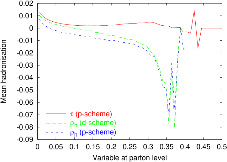
Figure 11: The hadronisation correction as a function of the value of the variable at parton level.

To help understand what is happening we have used Pythia to look at the mean hadronisation as a function of the value of the variable at parton level, figure 11. For the thrust, the hadronisation is fairly independent of the parton-level thrust value. For the heavy jet masses (in the massive and $p$-schemes) however the hadronisation correction is very negative for larger values of $\rho_{h}$ at parton level (we note that there are also very large event-by-event fluctuations in the hadronisation — this means that the hadronisation does not just cause a simple shift of the perturbative distribution). This feature may be at the root of the non-universality seen in the heavy jet mass, and needs to be understood — one explanation might be that when one hemisphere is perturbatively heavy, the phase-space that remains for further emissions is limited, and the only way of emitting non-perturbative radiation in the light-hemisphere is if some energy (and mass) is removed from the heavy hemisphere. However such a hypothesis would need to be placed on a more rigorous mathematical footing for it to be tested.

Such a phenomenon might also play a role in the wide-jet broadening, where it has been observed that the theoretically predicted distribution is too wide at larger values of $B_{W}$ [47].

References

- [1] B. R. Webber, Phys. Lett. B339 (1994) 148 [hep-ph/9408222].
- [2] B. R. Webber, in proceedings of the Summer School on Hadronic Aspects of Collider Physics, Zuoz, Switzerland, 1994, hep-ph/9411384.
- [3] Y. L. Dokshitzer and B. R. Webber, Phys. Lett. B352 (1995) 451 [hep-ph/9504219].
- [4] Y. L. Dokshitzer, G. Marchesini and B. R. Webber, Nucl. Phys. B469 (1996) 93 [hep-ph/9512336].
- [5] M. Dasgupta and B. R. Webber, Phys. Lett. B382 (1996) 273 [hep-ph/9604388].
-
[6]
G. P. Korchemsky and G. Sterman,
Nucl. Phys. B437 (1995) 415
[hep-ph/9411211];
G. P. Korchemsky, G. Oderda and G. Sterman, presented at 5th International Workshop on Deep Inelastic Scattering and QCD (DIS 97), Chicago, IL, April 1997 hep-ph/9708346;
G. P. Korchemsky and G. Sterman, Nucl. Phys. B 555 (1999) 335 [hep-ph/9902341]. -
[7]
R. Akhoury and V. I. Zakharov,
Phys. Lett. B357 (1995) 646
[hep-ph/9504248].
R. Akhoury and V. I. Zakharov, Nucl. Phys. B465 (1996) 295 [hep-ph/9507253]. - [8] M. Beneke and V. M. Braun, Nucl. Phys. B454 (1995) 253 [hep-ph/9506452].
- [9] P. Nason and M. H. Seymour, Nucl. Phys. B454 (1995) 291 [hep-ph/9506317].
- [10] M. Beneke, V. M. Braun and L. Magnea, Nucl. Phys. B497 (1997) 297 [hep-ph/9701309].
- [11] Y. L. Dokshitzer, A. Lucenti, G. Marchesini and G. P. Salam, Nucl. Phys. B511 (1998) 396 [hep-ph/9707532], erratum ibid. B593 (2001) 729.
- [12] Y. L. Dokshitzer, A. Lucenti, G. Marchesini and G. P. Salam, JHEP 9805 (1998) 003 [hep-ph/9802381].
- [13] M. Dasgupta and B. R. Webber, JHEP 9810 (1998) 001 [hep-ph/9809247].
-
[14]
M. Dasgupta, L. Magnea and G. Smye,
JHEP 9911 (1999) 025
[hep-ph/9911316];
G. Smye, hep-ph/0101323. - [15] Y. L. Dokshitzer, G. Marchesini and G. P. Salam, Eur. Phys. J. direct C3 (1999) 1 [hep-ph/9812487], erratum ibid. C1 (2001) 1.
- [16] E. Gardi and G. Grunberg, JHEP 9911 (1999) 016 [hep-ph/9908458].
- [17] Z. Trocsanyi, JHEP 0001 (2000) 014 [hep-ph/9911353].
- [18] G. P. Korchemsky and S. Tafat, JHEP 0010 (2000) 010 [hep-ph/0007005].
-
[19]
P. Abreu et al. (DELPHI Collaboration),
Phys. Lett. B456 (1999) 322;
P. A. Movilla Fernandez, O. Biebel, S. Bethke, S. Kluth and P. Pfeifenschneider (JADE Collaboration), Eur. Phys. J. C1 (1998) 461 [hep-ex/9708034];
M. Acciarri et al. (L3 Collaboration), Phys. Lett. B489 (2000) 65 [hep-ex/0005045];
H. Stenzel, MPI-PHE-99-09 Prepared for 34th Rencontres de Moriond: “QCD and Hadronic interactions”, Les Arcs, France, 20-27 Mar 1999;
ALEPH Collaboration, “QCD Measurements in e+e- Annihilations at Centre-of-Mass Energies between 189 and 202 GeV”, ALEPH 2000-044 CONF 2000-027; -
[20]
C. Adloff et al. (H1 Collaboration),
Phys. Lett. B406 (1997) 256
[hep-ex/9706002];
C. Adloff et al. (H1 Collaboration), Eur. Phys. J. C14 (2000) 255 [hep-ex/9912052], erratum ibid. C18 (2000) 417. - [21] DELPHI Collaboration, “The Running of the Strong Coupling and a Study of Power Corrections to Hadronic Event Shapes with the DELPHI Detector at LEP”, DELPHI 2000-116 CONF 415, July 2000.
-
[22]
G. J. McCance (for the H1 and ZEUS collaborations),
Talk given at 35th Rencontres de Moriond: QCD and High Energy
Hadronic Interactions (March 2000),
hep-ex/0008009;
H. Martyn (for the H1 and ZEUS Collaborations), Talk given at 30th International Conference on High-Energy Physics (ICHEP 2000), hep-ex/0010046. - [23] R.P. Feynman, ‘Photon Hadron Interactions’, W.A. Benjamin, New York (1972).
-
[24]
A. H. Mueller,
Phys. Lett. B104 (1981) 161;
B. I. Ermolaev and V. S. Fadin, JETP Lett. 33 (1981) 269;
Y. L. Dokshitzer, V. S. Fadin and V. A. Khoze, Z. Phys. C15 (1982) 325;
A. Bassetto, M. Ciafaloni, G. Marchesini and A. H. Mueller, Nucl. Phys. B207 (1982) 189;
A. Bassetto, M. Ciafaloni and G. Marchesini, Phys. Rept. 100 (1983) 201. - [25] G. Marchesini, B. R. Webber, G. Abbiendi, I. G. Knowles, M. H. Seymour and L. Stanco, Comput. Phys. Commun. 67 (1992) 465.
- [26] L. Lönnblad, Comput. Phys. Commun. 71 (1992) 15; we have use Ariadne version 4.08 converted to double precision to enable it to be interfaced to Pythia 6, instead of the older single-precision Jetset; As a consequence we use identical fragmentation models for Pythia and Ariadne.
-
[27]
T. Sjöstrand,
Comput. Phys. Commun. 82 (1994) 74;
T. Sjöstrand, P. Eden, C. Friberg, L. Lönnblad, G. Miu, S. Mrenna and E. Norrbin, hep-ph/0010017. - [28] Sergio Leone, Il Buono, il Brutto, il Cattivo, Italy 1966.
-
[29]
N. A. Sveshnikov and F. V. Tkachov,
Phys. Lett. B 382 (1996) 403
[hep-ph/9512370];
P. S. Cherzor and N. A. Sveshnikov, presented at 12th International Workshop High-Energy Physics and Quantum Field Theory (QFTHEP 97), Samara, Russia, September 1997, hep-ph/9710349;
F. V. Tkachov, hep-ph/9901444. - [30] Yu.L. Dokshitzer and S.I. Troyan, Proceedings of the XIX Winter School of the LNPI, volume 1, p. 144. Leningrad, 1984.
- [31] Ya.I. Azimov, Yu.L. Dokshitzer, V.A. Khoze and S.I. Troyan, Z. Phys. C27 (1985) 65.
- [32] V. A. Khoze, S. Lupia and W. Ochs, Eur. Phys. J. C5 (1998) 77 [hep-ph/9711392].
- [33] Yu.L. Dokshitzer, V.A. Khoze, A.H. Mueller and S.I. Troyan, Basics of Perturbative QCD, Editions Frontières, 1991, Gif-sur-Yvette, France.
- [34] A. H. Mueller, Nucl. Phys. B213 (1983) 85, erratum quoted ibid., B241 (1984) 141.
- [35] P. Abreu et al. (DELPHI Collaboration), Z. Phys. C73 (1996) 11.
-
[36]
D. Decamp et al. (ALEPH Collaboration),
Phys. Lett. B284 (1992) 163;
D. Buskulic et al. (ALEPH Collaboration), Z. Phys. C55 (1992) 209;
I. H. Park et al. (AMY Collaboration), Phys. Rev. Lett. 62 (1989) 1713;
Y. K. Li et al. (AMY Collaboration), Phys. Rev. D 41 (1990) 2675;
H. J. Behrend et al. (CELLO Collaboration), Z. Phys. C44 (1989) 63;
D. Bender et al. (HRS Collaboration), Phys. Rev. D 31 (1985) 1;
P. A. Movilla Fernandez, O. Biebel, S. Bethke, S. Kluth and P. Pfeifenschneider (JADE Collaboration), Eur. Phys. J. C1 (1998) 461 [hep-ex/9708034];
B. Adeva et al. (L3 Collaboration), Z. Phys. C55 (1992) 39;
M. Acciarri et al. (L3 Collaboration), Phys. Lett. B411 (1997) 339;
D. P. Barber et al. (Mark J Collaboration), Phys. Rev. Lett. 43 (1979) 830;
A. Petersen et al. (Mark II Collaboration), Phys. Rev. D 37 (1988) 1;
S. Bethke et al. (Mark II Collaboration), Z. Phys. C43 (1989) 325;
P. D. Acton et al. (OPAL Collaboration), Z. Phys. C59 (1993) 1;
G. Alexander et al. (OPAL Collaboration), Z. Phys. C72 (1996) 191;
K. Ackerstaff et al. (OPAL Collaboration), Z. Phys. C75 (1997) 193;
C. Berger et al. (PLUTO Collaboration), Z. Phys. C12 (1982) 297;
K. Abe et al. (SLD Collaboration), Phys. Rev. D 51 (1995) 962 [hep-ex/9501003];
W. Braunschweig et al. (TASSO Collaboration), Phys. Lett. B214 (1988) 286;
W. Braunschweig et al. (TASSO Collaboration), Z. Phys. C45 (1989) 11;
W. Braunschweig et al. (TASSO Collaboration), Z. Phys. C47 (1990) 187;
I. Adachi et al. (TOPAZ Collaboration), Phys. Lett. B227 (1989) 495;
K. Nagai et al. (TOPAZ Collaboration), Phys. Lett. B278 (1992) 506;
Y. Ohnishi et al. (TOPAZ Collaboration), Phys. Lett. B313 (1993) 475. - [37] P. Nason and B. R. Webber, Nucl. Phys. B421 (1994) 473, erratum ibid. B480 755 (1996).
- [38] P. Nason and C. Oleari, Nucl. Phys. B521 (1998) 237 [hep-ph/9709360].
- [39] C. Oleari, Ph.D. thesis, hep-ph/9802431.
- [40] G. Rodrigo, Nucl. Phys. Proc. Suppl. 54A (1997) 60 [hep-ph/9609213].
- [41] G. V. Rodrigo, Ph.D. thesis, hep-ph/9703359.
- [42] G. Rodrigo, A. Santamaria and M. Bilenkii, Phys. Rev. Lett. 79 (1997) 193 [hep-ph/9703358].
- [43] W. Bernreuther, A. Brandenburg and P. Uwer, Phys. Rev. Lett. 79 (1997) 189 [hep-ph/9703305].
- [44] A. Brandenburg and P. Uwer, Nucl. Phys. B515 (1998) 279 [hep-ph/9708350].
- [45] G. Abbiendi et al. (OPAL Collaboration), Eur. Phys. J. C11 (1999) 643 [hep-ex/9904013].
- [46] S. Catani and B. R. Webber, Phys. Lett. B427 (1998) 377 [hep-ph/9801350].
- [47] G. P. Salam and G. Zanderighi, Nucl. Phys. Proc. Suppl. 86 (2000) 430 [hep-ph/9909324].