$V_{cs}$ from Pure Leptonic Decays of $D_{s}$ with Radiative Corrections

Guo-Li Wanga,c, Tai-Fu Fengb,c and Chao-Hsi Changc
Abstract

The radiative corrections to the pure leptonic decay $D_{s}{\longrightarrow}{\ell}{{\nu}}_{\ell}$ up-to one-loop order is presented. We find the virtual photon loop corrections to DsβŸΆΟ„β€‹Ξ½Ο„βŸΆsubscriptπ·π‘ πœsubscript𝜈𝜏D_{s}{\longrightarrow}{\tau}{{\nu}}_{\tau} is negative and the corresponding branching ratio is larger than $3.51\times 10^{-3}$. Considering the possible experimental resolutions, our prediction of the radiative decay DsβŸΆΟ„β€‹Ξ½Ο„β€‹Ξ³βŸΆsubscriptπ·π‘ πœsubscriptπœˆπœπ›ΎD_{s}{\longrightarrow}{\tau}{{\nu}}_{\tau}\gamma is not so large as others, and the best radiative channel to determine the $V_{cs}$ or $f_{D_{s}}$ is DsβŸΆΞΌβ€‹Ξ½ΞΌβ€‹Ξ³βŸΆsubscriptπ·π‘ πœ‡subscriptπœˆπœ‡π›ΎD_{s}{\longrightarrow}{\mu}{{\nu}}_{\mu}{\gamma}.

$a$, Department of Physics, FuJian Normal University, FuZhou 350007, China

$b$, Department of Physics, NanKai University, TianJin 300070, China

$c$, Institute of Theoretical Physics, Academia Sinica, P.O.Box 2735, BeiJing 100080,China

PACS numbers:13.20.Fc, 12.39.Jh, 13.40.Ks

The pure-leptonic decay $D_{s}{\longrightarrow}{\ell}{{\nu}_{\ell}}$ can be used to determine the decay constant $f_{D_{s}}$ if the fundamental Cabibbo-Kobayashi-Maskawa matrix element $V_{cs}$ of Standard Model (SM) is known. Conversely if we know the value of decay constant $f_{D_{s}}$ from other method[1, 2, 3], these process also can be used to extract the matrix element $V_{cs}$. But there are the well known effect of helicity suppression we can see it by factor of $m_{\ell}^{2}/m_{D_{s}}^{2}$:

$$\Gamma(D_{s}{\longrightarrow}{\ell}{\overline{\nu}_{\ell}})={\frac{G_{F}^{2}}{8\pi}}|V_{cs}|^{2}f_{D_{s}}^{2}m_{D_{s}}^{3}{\frac{{m_{\ell}}^{2}}{{m_{D_{s}}}^{2}}}\left(1-{\frac{{m_{\ell}}^{2}}{{m_{D_{s}}}^{2}}}\right)^{2},$$ (1)

Of them only the process DsβŸΆΟ„β€‹Ξ½Ο„βŸΆsubscriptπ·π‘ πœsubscript𝜈𝜏D_{s}{\longrightarrow}{{\tau}}{\nu}_{\tau} is special, it does not suffer so much from the helicity suppression, and its branching ratio may reach to $4.5\%$ in SM. However the produced $\tau$ will decay promptly and one more neutrino is generated in the cascade decay at least, thus it makes the decay channel difficult to be observed. For the channels $D_{s}{\longrightarrow}{{e}}{\nu}_{e}$ and DsβŸΆΞΌβ€‹Ξ½ΞΌβŸΆsubscriptπ·π‘ πœ‡subscriptπœˆπœ‡D_{s}{\longrightarrow}{{\mu}}{\nu}_{\mu}, besides the small branching ratios, there are only one detected finial state, the measurement of such channels are very difficult.

Fortunately, having an extra real photon emitted in the leptonic decays, the radiative pure leptonic decays can escape from the suppression[4, 5, 6], furthermore, as pointed out in Ref.[7], with the extra photon to identify the decaying pseudoscalar meson $D_{s}$ in experiment from the backgrounds has advantages, since one more particle can be detected in the detector. Although the radiative corrections are suppressed by an extra electromagnetic coupling constant $\alpha$, it will not be suppressed by the helicity suppression. Therefore, the radiative decay may be comparable, even larger than the corresponding pure leptonic decays[4, 5, 6].

The radiative pure leptonic decays, theoretically, have infrared divergences and will be canceled with those from loop corrections of the pure leptonic decays. In all the existing calculation of radiative decays[4, 5, 6], this part is ignored, since they do not include the radiative corrections of the pure leptonic decays. In this paper, we are interested in considering the radiative decays and the pure leptonic decays with one-loop radiative corrections together. Since the process DsβŸΆΟ„β€‹Ξ½Ο„βŸΆsubscriptπ·π‘ πœsubscript𝜈𝜏D_{s}{\longrightarrow}{{\tau}}{\nu}_{\tau} dose not suffer the helicity suppression and has a large branching ratio, the corresponding loop correction(virtual photon) to these process should has a considerable larger branching ratio, at least comparing with the radiative decay, and can not be ignored.

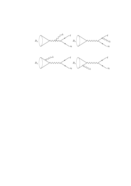
The contributions of the radiative decays are corresponding to the four diagrams in Fig.1. According to the constituent quark model which is formulated by Bethe-Salpeter (B.-S.) equation, the amplitude turns out to be the four terms $M_{i}(i=1,2,3,4)$:

$$M_{1}=Tr\left[\int\frac{d^{4}q}{(2\pi)^{4}}\chi(p,q)i\left(\frac{G_{F}m_{w}^{2}}{\sqrt{2}}\right)^{\frac{1}{2}}{\gamma}_{\mu}(1-\gamma_{5})V_{cs}\right]\times$$
$${\frac{i\left(-g^{\mu\nu}+\frac{p^{\mu}p^{\nu}}{m_{w}^{2}}\right)}{p^{2}-m_{w}^{2}}}ie[(p^{\prime}+p)_{\lambda}g_{\nu\rho}+(k-p^{\prime})_{\nu}g_{\rho\lambda}+(-p-k)_{\rho}g_{\nu\lambda}]{\epsilon}^{\lambda}\times$$
$$\frac{i\left(-g^{{\rho}{\sigma}}+\frac{(p-k)^{\rho}(p-k)^{\sigma}}{m_{w}^{2}}\right)}{(p-k)^{2}-m_{w}^{2}}\overline{\ell}\frac{ig}{2\sqrt{2}}\gamma_{\sigma}(1-{\gamma}_{5})\nu_{\ell},$$ (2)
$$M_{2}=Tr\left[\int\frac{d^{4}q}{(2\pi)^{4}}\chi(p,q)i\left(\frac{G_{F}m_{w}^{2}}{\sqrt{2}}\right)^{\frac{1}{2}}{\gamma}_{\mu}(1-\gamma_{5})V_{cs}\right]{\frac{i\left(-g^{\mu\nu}+\frac{p^{\mu}p^{\nu}}{m_{w}^{2}}\right)}{p^{2}-m_{w}^{2}}}$$
$$\times\overline{\ell}(-ie)\not\!{\epsilon}\frac{i}{\not\!{k}_{\ell}-m_{\ell}}\frac{ig}{2\sqrt{2}}\gamma_{\nu}(1-{\gamma}_{5})\nu_{\ell},$$ (3)
M3=T​r​[∫d4​q(2​π)4​χ​(p,q)​i​(GF​mw22)12​γμ​(1βˆ’Ξ³5)​Vc​s​imsms+mc​​p+​qβˆ’β€‹kβˆ’ms​(βˆ’i​e3​​ϡ)]subscript𝑀3π‘‡π‘Ÿdelimited-[]superscript𝑑4π‘žsuperscript2πœ‹4πœ’π‘π‘žπ‘–superscriptsubscript𝐺𝐹superscriptsubscriptπ‘šπ‘€2212subscriptπ›Ύπœ‡1subscript𝛾5subscript𝑉𝑐𝑠𝑖subscriptπ‘šπ‘ subscriptπ‘šπ‘ subscriptπ‘šπ‘π‘π‘žπ‘˜subscriptπ‘šπ‘ π‘–π‘’3italic-Ο΅M_{3}=Tr\left[\int\frac{d^{4}q}{(2\pi)^{4}}\chi(p,q)i\left(\frac{G_{F}m_{w}^{2}}{\sqrt{2}}\right)^{\frac{1}{2}}{\gamma}_{\mu}(1-\gamma_{5})V_{cs}\frac{i}{\frac{m_{s}}{m_{s}+m_{c}}\not\!{p}+\not\!{q}-\not\!{k}-m_{s}}\left(-i\frac{e}{3}\not\!{\epsilon}\right)\right]
$$\times\frac{i\left(-g^{{\mu}{\sigma}}+\frac{(p-k)^{\mu}(p-k)^{\sigma}}{m_{w}^{2}}\right)}{(p-k)^{2}-m_{w}^{2}}\overline{\ell}\frac{ig}{2\sqrt{2}}\gamma_{\sigma}(1-{\gamma}_{5})\nu_{\ell},$$ (4)
M4=T​r​[∫d4​q(2​π)4​χ​(p,q)​(i​2​e3​​ϡ)​iβˆ’(mcms+mc​​pβˆ’β€‹qβˆ’β€‹k)βˆ’mc​i​(GF​mw22)12​γμ​(1βˆ’Ξ³5)​Vc​s]subscript𝑀4π‘‡π‘Ÿdelimited-[]superscript𝑑4π‘žsuperscript2πœ‹4πœ’π‘π‘žπ‘–2𝑒3italic-ϡ𝑖subscriptπ‘šπ‘subscriptπ‘šπ‘ subscriptπ‘šπ‘π‘π‘žπ‘˜subscriptπ‘šπ‘π‘–superscriptsubscript𝐺𝐹superscriptsubscriptπ‘šπ‘€2212subscriptπ›Ύπœ‡1subscript𝛾5subscript𝑉𝑐𝑠M_{4}=Tr\left[\int\frac{d^{4}q}{(2\pi)^{4}}\chi(p,q)\left(i\frac{2e}{3}\not\!{\epsilon}\right)\frac{i}{-(\frac{m_{c}}{m_{s}+m_{c}}\not\!{p}-\not\!{q}-\not\!{k})-m_{c}}i\left(\frac{G_{F}m_{w}^{2}}{\sqrt{2}}\right)^{\frac{1}{2}}{\gamma}_{\mu}(1-\gamma_{5})V_{cs}\right]
$$\times\frac{i\left(-g^{{\mu}{\sigma}}+\frac{(p-k)^{\mu}(p-k)^{\sigma}}{m_{w}^{2}}\right)}{(p-k)^{2}-m_{w}^{2}}\overline{\ell}\frac{ig}{2\sqrt{2}}\gamma_{\sigma}(1-{\gamma}_{5})\nu_{\ell},$$ (5)

where $\chi(p,q)$ is Bethe-Salpeter wave function of the meson $D_{s}$; $p$ is the momentum of $D_{s}$; ${\epsilon},k$ are the polarization vector and momentum of the emitted photon.

As the $D_{s}$ meson is a nonrelativistic S-wave bound state in nature, higher order relativistic corrections may be small, being the first order approximation for a $S$-wave state, we ignore $q$ dependence in amplitude and in the $D_{s}$ wave-function and write the wave function of the meson $D_{s}$ as:

$$\int\frac{d^{4}q}{(2\pi)^{4}}\chi(p,q)=\frac{\gamma_{5}({/}\!\!\!{p}{+m})}{2\sqrt{m}}\psi(0).$$

Here $\psi(0)$ is the wave function at origin in the coordinate space, and by definitions it connects to the decay constant $f_{D_{s}}$:

$$\psi(0)=2\sqrt{m}f_{D_{s}},$$

where m is the mass of $D_{s}$ meson. Moreover we note that for convenience we take unitary gauge for weak boson to do the calculations throughout the paper.

There is infrared infinity when performing phase space integral about the square of matrix element at the soft photon limit. It is known that the infrared infinity can be cancelled completely by that of the loop corrections to the corresponding pure leptonic decay Ds→ℓ​ν→subscriptπ·π‘ β„“πœˆD_{s}\to\ell\nu.

If Feynman gauge for photon is taken, the amplitude of loop corrections corresponding to the box diagrams (a), (b)[7] can be written as:

M(2)​(a)=23​e​Aβ€‹βˆ«d4​l(2​π)4​[βˆ’4​i​Ρα​μ​β​ν​pα​lΞ²βˆ’4​(pμ​lΞ½βˆ’pβ‹…l​gμ​ν+pν​lΞΌ)+8​mcms+mc​pμ​pΞ½l2​(l2βˆ’2​pβ‹…lβˆ’mw2)​(l2βˆ’2​mcms+mc​pβ‹…l)​[l2βˆ’2​lβ‹…(pβˆ’k2)]]subscript𝑀2π‘Ž23𝑒𝐴superscript𝑑4𝑙superscript2πœ‹4delimited-[]4𝑖superscriptπœ€π›Όπœ‡π›½πœˆsubscript𝑝𝛼subscript𝑙𝛽4subscriptπ‘πœ‡subscriptπ‘™πœˆβ‹…π‘π‘™subscriptπ‘”πœ‡πœˆsubscriptπ‘πœˆsubscriptπ‘™πœ‡8subscriptπ‘šπ‘subscriptπ‘šπ‘ subscriptπ‘šπ‘subscriptπ‘πœ‡subscriptπ‘πœˆsuperscript𝑙2superscript𝑙2β‹…2𝑝𝑙superscriptsubscriptπ‘šπ‘€2superscript𝑙2β‹…2subscriptπ‘šπ‘subscriptπ‘šπ‘ subscriptπ‘šπ‘π‘π‘™delimited-[]superscript𝑙2β‹…2𝑙𝑝subscriptπ‘˜2M_{(2)}(a)={\frac{2}{3}}eA\int\frac{d^{4}l}{(2\pi)^{4}}\left[\frac{-4i\varepsilon^{\alpha\mu\beta\nu}p_{\alpha}l_{\beta}-4(p_{\mu}l_{\nu}-{p\cdot l}g_{\mu\nu}+p_{\nu}l_{\mu})+\frac{8m_{c}}{m_{s}+m_{c}}p_{\mu}p_{\nu}}{l^{2}(l^{2}-2p\cdot l-m_{w}^{2})(l^{2}-{\frac{2m_{c}}{m_{s}+m_{c}}}p\cdot{l})[l^{2}-2l\cdot{(p-k_{2})}]}\right]
$$\times\overline{\ell}[2(p-k_{2})_{\mu}-\gamma_{\mu}{\not\!{l}}](-\gamma_{\nu})(1-\gamma_{5})\nu_{\ell},$$ (6)
M(2)​(b)=βˆ’13​e​Aβ€‹βˆ«d4​l(2​π)4​[βˆ’4​i​Ρα​μ​β​ν​pα​lΞ²+4​(pμ​lΞ½βˆ’pβ‹…l​gμ​ν+pν​lΞΌ)βˆ’8​msms+mc​pμ​pΞ½l2​(l2βˆ’2​pβ‹…lβˆ’mw2)​(l2βˆ’2​msms+mc​pβ‹…l)​[l2βˆ’2​lβ‹…(pβˆ’k2)]]subscript𝑀2𝑏13𝑒𝐴superscript𝑑4𝑙superscript2πœ‹4delimited-[]4𝑖superscriptπœ€π›Όπœ‡π›½πœˆsubscript𝑝𝛼subscript𝑙𝛽4subscriptπ‘πœ‡subscriptπ‘™πœˆβ‹…π‘π‘™subscriptπ‘”πœ‡πœˆsubscriptπ‘πœˆsubscriptπ‘™πœ‡8subscriptπ‘šπ‘ subscriptπ‘šπ‘ subscriptπ‘šπ‘subscriptπ‘πœ‡subscriptπ‘πœˆsuperscript𝑙2superscript𝑙2β‹…2𝑝𝑙superscriptsubscriptπ‘šπ‘€2superscript𝑙2β‹…2subscriptπ‘šπ‘ subscriptπ‘šπ‘ subscriptπ‘šπ‘π‘π‘™delimited-[]superscript𝑙2β‹…2𝑙𝑝subscriptπ‘˜2M_{(2)}(b)={-\frac{1}{3}}eA\int\frac{d^{4}l}{(2\pi)^{4}}\left[\frac{-4i\varepsilon^{\alpha\mu\beta\nu}p_{\alpha}l_{\beta}+4(p_{\mu}l_{\nu}-{p\cdot l}g_{\mu\nu}+p_{\nu}l_{\mu})-\frac{8m_{s}}{m_{s}+m_{c}}p_{\mu}p_{\nu}}{l^{2}(l^{2}-2p\cdot l-m_{w}^{2})(l^{2}-{\frac{2m_{s}}{m_{s}+m_{c}}}p\cdot{l})[l^{2}-2l\cdot{(p-k_{2})}]}\right]
$$\times\overline{\ell}[2(p-k_{2})_{\mu}-\gamma_{\mu}{\not\!{l}}](-\gamma_{\nu})(1-\gamma_{5})\nu_{\ell},$$ (7)

where the $l$, $k_{2}$ denote the momenta of the loop and the neutrino respectively. These two terms also have infrared infinity when integrating out the loop momentum $l$.

After doing the on-mass-shell subtraction, the terms corresponding to vertex and self-energy diagrams (c), (d), (e), (f)[7] can be written as:

$$M_{(2)}(c+d+e+f)=\frac{ieA}{4\pi^{2}}\overline{\ell}{\not\!p}(1-\gamma_{5})\nu_{\ell}\times\left[ln(4)-\frac{8}{9}+\frac{2}{9}{\frac{m_{s}-m_{c}}{m_{s}+m_{c}}}ln\left(\frac{m_{s}}{m_{c}}\right)\right.$$
+(29+89​mcms+mc)​l​n​(ms+mcms)+(89+89​mcms+mc)​l​n​(ms+mcmc)2989subscriptπ‘šπ‘subscriptπ‘šπ‘ subscriptπ‘šπ‘π‘™π‘›subscriptπ‘šπ‘ subscriptπ‘šπ‘subscriptπ‘šπ‘ 8989subscriptπ‘šπ‘subscriptπ‘šπ‘ subscriptπ‘šπ‘π‘™π‘›subscriptπ‘šπ‘ subscriptπ‘šπ‘subscriptπ‘šπ‘+\left(\frac{2}{9}+\frac{8}{9}{\frac{m_{c}}{m_{s}+m_{c}}}\right)ln\left(\frac{m_{s}+m_{c}}{m_{s}}\right)+\left(\frac{8}{9}+\frac{8}{9}{\frac{m_{c}}{m_{s}+m_{c}}}\right)ln\left(\frac{m_{s}+m_{c}}{m_{c}}\right)
$$+\left.\frac{2}{\varepsilon_{I}}-2\gamma+ln\left(\frac{4\pi\mu^{2}}{m^{2}}\right)+ln\left(\frac{4\pi\mu^{2}}{m_{e}^{2}}\right)\right].$$ (8)

where $A$ is:

$$A=\frac{f_{D_{s}}\left(\frac{G_{F}m_{w}^{2}}{\sqrt{2}}\right)^{\frac{1}{2}}V_{cs}eg}{2\sqrt{2}}=f_{D_{s}}\left(\frac{G_{F}m_{w}^{2}}{\sqrt{2}}\right)V_{cs}e.$$

The other loop diagrams(we do not show them) always have a further suppression factor $m^{2}/{m_{w}}^{2}$ to compare with the loop diagrams we considered, and there is no infrared infinity in these loop diagrams, we can ignored their contributions safely. Furthermore we should note that in our calculations throughout the paper, the dimensional regularization to regularize both infrared and ultraviolet divergences is adopted, while the on-mass-shell renormalization for the ultraviolet divergence is used.

Detail cancellation of infrared divergence is given in Ref[8]. Here we simply show the results. The β€˜whole’ leptonic decay branching ratios, i.e., the sum of the corresponding radiative decay branching ratios and the corresponding pure leptonic decay branching ratios with radiative corrections, and put them in Table (1). The reason we put the radiative decay and the pure leptonic decay with radiative corrections together is to make the branching ratios not to depend on the experimental resolution for a soft photon. For comparison, the branching ratios of each pure leptonic decay at tree level is also put in Table (1). The values for the parameters $\alpha=1/132$, $|V_{cs}|=0.974$[9], $m_{D_{s}}=1.9686$ GeV, ms=0.5subscriptπ‘šπ‘ 0.5m_{s}=0.5 GeV, $m_{c}=1.7$ GeV, $f_{D_{s}}=0.24$ GeV[10] and the lifetime $\tau(D_{s})=0.469\times 10^{-12}s$[9].

Table (1) Branching Ratios of the β€˜Whole’ and Tree Lever Leptonic Decays

β€˜whole’ tree
$B_{e}(10^{-5})$ 2.56 0.0108
$B_{\mu}(10^{-3})$ 4.706 4.605
$B_{\tau}(10^{-2})$ 4.138 4.489

We can see that, the β€˜whole’ decay branching ratios $Br_{e}$ and $Br_{\mu}$ are larger than the corresponding branching ratios of tree lever, while the β€˜whole’ $Br_{\tau}$ is smaller than the tree lever one. It means the contributions of loop corrections are negative, the dominate contributions of first order corrections to the pure leptonic $D_{s}$ decays are radiative decays when the lepton is $e$ or $\mu$, and is loop corrections when the lepton is $\tau$. So, the loop contributions are important for the decays Ds→μ​νμ→subscriptπ·π‘ πœ‡subscriptπœˆπœ‡D_{s}\to\mu\nu_{\mu} and Ds→τ​ντ→subscriptπ·π‘ πœsubscript𝜈𝜏D_{s}\to\tau\nu_{\tau}, especially for the later. Through Table (1), we obtained that the rediative decay has a branching ratio B​r​(Ds→μ​νμ​γ)>1.01Γ—10βˆ’4π΅π‘Ÿβ†’subscriptπ·π‘ πœ‡subscriptπœˆπœ‡π›Ύ1.01superscript104Br(D_{s}\to\mu\nu_{\mu}\gamma)>1.01\times 10^{-4} and the loop correction to Ds→τ​ντ→subscriptπ·π‘ πœsubscript𝜈𝜏D_{s}\to\tau\nu_{\tau} has a branching ratio $Br>3.51\times 10^{-3}$.

To see the contributions of the radiative decays precisely we present the radiative decay branching ratios with a cut of the photon energy, i.e., the branching ratios of the radiative decays Dsβ†’l​ν​γ→subscriptπ·π‘ π‘™πœˆπ›ΎD_{s}\rightarrow l\nu\gamma with the photon energy $E_{\gamma}\geq k_{min}$ as the follows: $k_{min}=0.00001$ GeV, $k_{min}=0.0001$ GeV, $k_{min}=0.001$ GeV, $k_{min}=0.01$ GeV and $k_{min}=0.1$ GeV respectively in Table (2). We also show the existing results of other methods in the same table.

Table (2): The Radiative Decay branching ratios with cuts of the photon momentum and the results of Ref[4, 5, 6]

$k_{min}$ $Br_{e}$ $Br_{\mu}$ $Br_{\tau}$
GeV $10^{-5}$ $10^{-4}$ $10^{-6}$
0.00001 2.552 4.901 6.336
0.0001 2.552 3.908 4.597
0.001 2.551 2.915 2.868
0.01 2.549 1.927 1.217
0.1 2.475 0.971 0.727
Ref[4] 10 1 $-$
Ref[5] 17 1.7 $-$
Ref[6] 7.7 2.6 320

Considering the possible experimental resolutions of photon, our prediction of the radiative decay branching ratios $Br(D_{s}\to e\nu_{e}\gamma)$ and B​r​(Ds→μ​νμ​γ)π΅π‘Ÿβ†’subscriptπ·π‘ πœ‡subscriptπœˆπœ‡π›ΎBr(D_{s}\to\mu\nu_{\mu}\gamma) are close to the values in Ref[4, 5, 6], but our prediction of B​r​(Ds→τ​ντ​γ)π΅π‘Ÿβ†’subscriptπ·π‘ πœsubscriptπœˆπœπ›ΎBr(D_{s}\to\tau\nu_{\tau}\gamma) is much smaller than the one in Ref[6]. In our model, if we using a smaller cut $k_{min}$, then obtained a larger $Br(D_{s}\to\ell\nu_{\ell}\gamma)$, because the decay widths depend on L​o​g​(km​i​n)​[8]πΏπ‘œπ‘”subscriptπ‘˜π‘šπ‘–π‘›[8]Log(k_{min})\cite[cite]{[\@@bibref{}{me}{}{}]}, the change of branching ratios will be not so much on the selection of $k_{min}$, we can see this in Table (2), and for another example, if $k_{min}=1.0\times 10^{-10}$ GeV, then we obtain $Br(D_{s}\to e\nu_{e}\gamma)=3.59\times 10^{-5}$, B​r​(Ds→μ​νμ​γ)=1.38Γ—10βˆ’3π΅π‘Ÿβ†’subscriptπ·π‘ πœ‡subscriptπœˆπœ‡π›Ύ1.38superscript103Br(D_{s}\to\mu\nu_{\mu}\gamma)=1.38\times 10^{-3}, B​r​(Ds→τ​ντ​γ)=2.11Γ—10βˆ’5π΅π‘Ÿβ†’subscriptπ·π‘ πœsubscriptπœˆπœπ›Ύ2.11superscript105Br(D_{s}\to\tau\nu_{\tau}\gamma)=2.11\times 10^{-5}, but so small a $k_{min}$, it is very difficult in experiment. We can conclude that the best radiative decay channel is easy to search in experiment is Ds→μ​νμ​γ→subscriptπ·π‘ πœ‡subscriptπœˆπœ‡π›ΎD_{s}\to\mu\nu_{\mu}\gamma.

For the convenience to compare with experiments, we present the photon spectrum of the radiative decays in Fig.2 and Fig.3. In addition, we should note that the widths are quite sensitive to the decay constant $f_{D_{s}}$, and are sensitive to the values of the quark masses mssubscriptπ‘šπ‘ m_{s} and $m_{c}$.

References

  • [1] As.Abada et al., Nucl. Phys. B376 (1992) 172.
  • [2] C.R.Allton et al., APE Collaboration, Nucl. Phys. B(Proc. Suppl.)34 (1993) 465.
  • [3] C.W.Bernard et al., Phys. Rev. D49 (1994) 2536.
  • [4] Gustavo Burdman,T.Goldman and Daniel Wyler, Phys. Rev. D51 (1995) 111.
  • [5] D.Arwood, G.Eilam and A.Soni, Mod. Phys. Lett. A11 (1996) 1061.
  • [6] C.Q.Geng,C.C.Lih and Wei-Min Zhang, hep-ph/0012066.
  • [7] C.-H. Chang, C-D LΓΌ, G.-L. Wang and H.-S. Zong, Phys. Rev. D60 (1999) 114013.
  • [8] Guo-Li Wang et al., unpublished.
  • [9] D.E.Groom et al., The European Physical Journal C15 (2000) 1.
  • [10] C.R.Allton et al., APE Collaboration, Nucl. Phys. B(Proc. Suppl.) 34 (1993) 456.
Refer to caption
Figure 1: Diagrams for DsβŸΆβ„“β€‹Ξ½β€‹Ξ³βŸΆsubscriptπ·π‘ β„“πœˆπ›ΎD_{s}\longrightarrow\ell\nu\gamma.
Refer to caption
Figure 2: Photon energy spectra of radiative decays $D_{s}\longrightarrow\ell{\nu_{\ell}}\gamma(\ell=e,\mu)$.
Refer to caption
Figure 3: Photon energy spectra of radiative decays DsβŸΆΟ„β€‹Ξ½Ο„β€‹Ξ³βŸΆsubscriptπ·π‘ πœsubscriptπœˆπœπ›ΎD_{s}\longrightarrow\tau{\nu_{\tau}}\gamma.