Abstract

We extract the $S$-matrix element for dipole-proton scattering using the data on diffractive electroproduction of vector mesons at HERA. By considering the full $t$ dependence of this process we are able to reliably unfold the profile of the $S$-matrix for impact parameter values $b>0.3\,\rm fm$ . We show that the results depend only weakly on the choice of the form for the vector meson wave function. We relate this result to the discussion about possible saturation effects at HERA.

Introduction

One of the key issues in deeply inelastic scattering and deeply inelastic diffraction is whether parton saturation effects are present in the HERA energy regime. The answer to this question has important implications for our understanding of the very early stages of relativistic heavy ion collisions where parton saturation would result in the production of a high density and high field strength, $F_{\mu\nu}\sim 1/{\sqrt{\alpha_{s}}}\ ,$ state of QCD. Such a state would be a new and exciting regime of nonperturbative but small coupling QCD.

Parton saturation can be viewed as a manifestation of unitarity limits being reached. However, unitarity limits are difficult to see directly in deep inelastic scattering and diffraction. Thus, most studies of parton saturation at HERA have been done in terms of models which explicitly impose unitarity at moderate $Q^{2}$ and small $x$. The most widely used such model is that of Golec-Biernat and Wüsthoff [1] where the $S$-matrix for the scattering of a dipole of separation $r$ on a proton is given by $S=e^{-r^{2}Q_{s}^{2}/4}$ with the saturation momentum, $Q_{s}^{2},$ depending on the energy of the scattering. The fact that the Golec-Biernat Wüsthoff model and its generalization work so well at HERA is perhaps some evidence that deep inelastic scattering, and especially diffraction, have reached unitarity limits.

It would be nice to see the attainment of unitarity limits directly without having to use a model. This is not an easy task. Recall that in proton-proton scattering the energy dependence of total and elastic cross sections changes little between ISR and Tevatron energies. The near saturation of unitarity limits was found in proton-proton scattering only when Amaldi and Schubert [2] evaluated the proton-proton elastic scattering amplitude in impact parameter space and found near blackness for small impact parameters.

Vector meson production seems to be the best process from which to extract the dipole proton elastic scattering amplitude. For example, it is easy to check that our procedure (see Eqs. (4)-(12) below) would not work for the total diffractive cross section because there is not a single definite state produced, a condition which seems necessary in the way we proceed.

In this paper we copy the Amaldi-Schubert analysis in order to determine the dipole-proton scattering amplitude in impact parameter space in terms of diffractive $\rho-$production data at HERA. Recall that diffractive electroproduction of a $\rho-$meson can be viewed in terms of the following sequence of transitions: (i) The virtual photon goes into a quark-antiquark pair (dipole). (ii) The dipole scatters elastically on the proton. (iii) The dipole then goes into a $\rho-$meson. Thus $\rho-$electroproduction naturally carries information on the dipole-quark elastic scattering amplitude. The main uncertainty is in the wavefunction of the $\rho-$meson which appears to be reasonably well constrained by previous phenomenology.

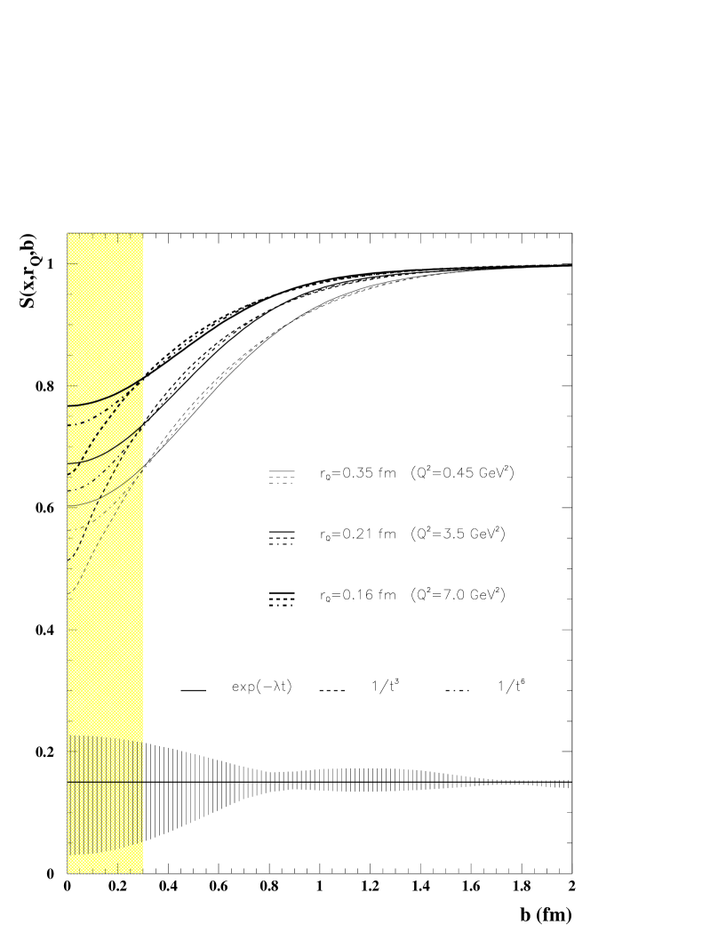
Figure 6: $S$-matrix for dipole-proton scattering as a function of impact parameter $b$. Three different $Q^{2}$ are considered, corresponding to three typical values for the size of the interacting dipole (which are estimated according to $r_{Q}\equiv e^{<\log r>_{p}}$). For each value of $Q^{2}$, the curves corresponding to three extrapolations of the data for $t>0.6\;\mbox{GeV}^{2}$ are shown. The shaded band indicates the region of impact parameter $b$ where the choice of this extrapolation is crucial, and thus where our extraction is not reliable. The hashed band on the bottom is an estimate of the errors due to the experimental uncertainties on $d\sigma/dt|_{t=0}$ and on $B(t)$ (for $t<0.6\,\mbox{GeV}^{2}$).

The dipole-proton $S$-matrix which we extract as a function of impact parameter is averaged over the dipole sizes which naturally appear in the $\gamma^{\ast}$ and $\rho-$meson wavefunctions. This averaging does not affect the fact that for weak interactions $S$ is near 1 and for strong interactions $S$  is near zero. Thus the smallness of $S$ is a measure of how close one is to the unitarity limit, $S=0.$ Perhaps the best way to measure how close the dipole-proton scattering is to the unitarity limit is to note that $\langle 1-S^{2}\rangle\geq 1-\langle S\rangle^{2}$ gives the probability that a dipole passing the proton will induce an inelastic reaction at the impact parameter in question ($\langle\cdot\cdot\cdot\rangle$ denotes the average over dipole sizes as explained in Eq. (11)). From our analysis this probability is likely significantly greater than $1/2$ for $Q^{2}\leq 2\,\mbox{GeV}^{2}$ and for $b$ near zero (see Fig. 6), although better large momentum transfer data would be needed to definitively determine $S$ at $b\approx 0.$ Thus, it is likely that saturation effects are important in this low $Q^{2}$ regime. Our estimate of $Q_{s}^{2}$ is about $1-1.5\,\mbox{GeV}^{2}$ at $b\approx 0.3$ fm, although this estimate has large uncertainties because it depends on knowing the average dipole size as a function of $Q^{2}.$ Finally, we determine the total dipole-proton cross sections for $x\approx 10^{-4}$ to be 14.9, 10.6 and 7.5 mb at $Q^{2}=0.45,3.5$ and $7\,\mbox{GeV}^{2}$ respectively.

The outline of the paper is as follows: in section 1 we establish the relation between the $S$-matrix for dipole-proton scattering averaged over the distribution of dipole sizes and the diffractive differential cross section for electroproduction of vector mesons. Due to the particular properties of this distribution, this formula translates into a method of determining the $S$-matrix profile in impact parameter space for a dipole of given size $r$. The only theoretical input needed is the vector meson wave function. In section 2 we discuss the parametrizations for the wave functions that we used, and we study in detail the model independence of our procedure. In section 3 we apply this method to the analysis of the available HERA data and present our main results on the $S$-matrix profile in impact parameter space. We discuss the uncertainties due to the experimental errors on the measured cross section and due to the lack of data in the high $t$ region. We also discuss the possible implications for studies of saturation effects at high energies. Finally, in section 4 we state the summary of our results. We append some more technical points.

1 Dipole-proton $S$-matrix and diffractive meson production cross section

We consider the process of diffractive production of a vector meson, $\gamma^{*}\!-\!p\rightarrow V\!-\!p$, shown in Fig. 1. We adopt here the dipole formulation [3, 4] in which the virtual photon $\gamma^{*}$ fluctuates into a $q\bar{q}$ pair (dipole) which subsequently interacts elastically with a proton, and eventually forms a meson bound state. This picture is justified at high center-of-mass energy of the $\gamma^{*}p$ system, since in this regime it is guaranteed that these successive processes are clearly separated in time. We assume that the energy is sufficiently high so that $s$-channel helicity conservation holds to a good accuracy, and we limit ourselves to the case of longitudinal vector meson production. The kinematics of this process is shown in Fig. 1: we define the 2-momentum transfer ${\mathbf{\Delta}}$ related to the Mandelstam variable $t$ by $t=-{\mathbf{\Delta}}^{2}$. $Q^{2}=-q^{2}$ and $x=Q^{2}/(2P\cdot q)$ are as usual the virtuality of the photon and the Bjorken variable, respectively.

In this framework, the amplitude ${\mathcal{A}}_{\mbox{\footnotesize el}}(x,{\mathbf{\Delta}},Q)$ for the scattering can be written in the following factorized form:

$${\mathcal{A}}_{\mbox{\footnotesize el}}(x,{\mathbf{\Delta}},Q)=\sum_{h,\bar{h}}\int d^{2}\mathbf{r}\,dz\,\psi_{\gamma^{*}}^{h,\bar{h}*}(z,{\mathbf{r}};Q)\,A_{\mbox{\footnotesize el}}^{q\bar{q}-p}(x,{\mathbf{r}},{\mathbf{\Delta}})\,\psi^{h,\bar{h}}_{V}(z,{\mathbf{r}})\;,$$ (1)

where $A_{\mbox{\footnotesize el}}^{q\bar{q}-p}(x,{\mathbf{r}},{\mathbf{\Delta}})$ is the elementary amplitude for the elastic scattering of a dipole of size ${\mathbf{r}}$ on the proton. $\psi^{h,\bar{h}}_{\gamma^{*}}$ is the photon light-cone wave function projected onto a state made of a quark-antiquark pair of charges $e_{q}$, masses $m_{q}$ and respective helicities $h$ and $\bar{h}$. This function is computed in first order light-cone perturbation theory of quantum electrodynamics, and for the longitudinally polarized virtual photon, it reads [3, 5]

$$\psi^{h,\bar{h}}_{\gamma^{*}}(z,{\mathbf{r}};Q)=\delta_{h,-\bar{h}}\ {e_{q}\over\sqrt{4\pi}}\ \frac{\sqrt{N_{c}}}{2\pi}2z(1\!-\!z)Q\,K_{0}(\varepsilon r)\ ,$$ (2)

where

$$\varepsilon^{2}=Q^{2}z(1-z)+m_{q}^{2}\ .$$ (3)

Similarly, $\psi^{h,\bar{h}}_{V}$ is the wave function of the vector meson produced in the final state. We discuss it in more detail in the next section. The variable $z$ in Eq. (1) is the fraction of longitudinal momentum of the virtual photon carried by the quark.

The amplitude is normalized in such a way that the differential cross section for the full process is

$${d\sigma\over dt}={1\over 16\pi}|{\mathcal{A}}_{\mbox{\footnotesize el}}(x,{\mathbf{\Delta}},Q)|^{2}\;.$$ (4)

Furthermore, the elementary amplitude $A_{\mbox{\footnotesize el}}^{q\bar{q}-p}(x,{\mathbf{r}},{\mathbf{\Delta}})$ can be related to the $S$-matrix element $S(x,{\mathbf{r}},{\mathbf{b}})$ for the scattering of a dipole of size ${\mathbf{r}}$ at impact parameter ${\mathbf{b}}$ [6]

$$A_{\mbox{\footnotesize el}}^{q\bar{q}-p}(x,{\mathbf{r}},{\mathbf{\Delta}})=\int d^{2}{\mathbf{b}}\,{{\tilde{A}}_{\mbox{\footnotesize el}}}^{q\bar{q}-p}(x,{\mathbf{r}},{\mathbf{b}})e^{i\mathbf{b}{\mathbf{\Delta}}}=2\int d^{2}{\mathbf{b}}\,[1-S(x,{\mathbf{r}},\mathbf{b})]e^{i\mathbf{b}{\mathbf{\Delta}}}\ .$$ (5)

We can check briefly the consistency of this formula, which defines $S(x,{\mathbf{r}},{\mathbf{b}})$ (see Ref. [7]). In the standard normalizations adopted here for the amplitudes, the optical theorem takes the form $\sigma_{\mbox{\footnotesize tot}}^{q\bar{q}-p}(x,{\mathbf{r}})={\mathcal{I}}m\,iA_{\mbox{\footnotesize el}}^{q\bar{q}-p}(x,{\mathbf{r}},{\mathbf{\Delta}}\!=\!0)$. Using formula (5), this relation translates into the following expression for the total dipole-proton cross section:

$$\sigma_{\footnotesize\rm tot}^{q\bar{q}-p}(x,\mathbf{r})=2\int d^{2}{\mathbf{b}}\,(1-{\mathcal{R}}e\,S(x,\mathbf{r},\mathbf{b}))\ .$$ (6)

On the other hand, taking the amplitude (5) squared, dividing it by the flux factor and integrating it over phase space, it is easy to see that the elastic cross section is given by

$$\sigma_{\footnotesize\rm el}^{q\bar{q}-p}(x,\mathbf{r})=\phantom{2}\int d^{2}{\mathbf{b}}\,\left|1-S(x,\mathbf{r},\mathbf{b})\right|^{2}\ .$$ (7)

When $S=0$, the unitarity limit is reached which is equivalent to the scattering on a black body. One sees from formulae (6) and (7) that the elastic cross section is half the total one, as it should be. This justifies the consistency of the normalization adopted for $S(x,{\mathbf{r}},{\mathbf{b}})$ in Eq. (5). We will assume in the following that $iA_{\mbox{\footnotesize el}}^{q\bar{q}-p}(x,{\mathbf{r}},{\mathbf{\Delta}})$ is purely imaginary, i.e. that $S(x,{\mathbf{r}},{\mathbf{b}})$ is real.

The main goal of this paper is to extract $S(x,{\mathbf{r}},{\mathbf{b}})$ taking advantage of the present experimental knowledge of the cross section for diffractive vector meson production, see Eq. (1). To this aim we express the amplitude which appears in Eqs. (1,4) by means of $S(x,{\mathbf{r}},{\mathbf{b}})$ using relation (5). Then we take the inverse Fourier transform of the square root of Eq.(4), which gives

$$\int{d^{2}{\mathbf{\Delta}}\over(2\pi)^{2}}\,\sqrt{{d\sigma\over dt}}e^{-i{\mathbf{\Delta}}{\mathbf{b}}}\;=\;{1\over\sqrt{16\pi}}\,\sum_{h,\bar{h}}\;\int d^{2}{\mathbf{r}}\,dz\,\psi_{\gamma^{*}}^{h,\bar{h}*}(z,{\mathbf{r}},Q)\,2\,[1-S(x,{\mathbf{r}},{\mathbf{b}})]\,\psi_{V}^{h,\bar{h}}(z,{\mathbf{r}})\ .$$ (8)

In the following we suppress the angular dependence of the $S$-matrix since in this process one is only sensitive to the quantities which are angular averaged. We single out the (logarithmic) distribution of dipole sizes at the photon vertex, which is the overlap between the photon and the meson wave functions

$$p(r,Q)\equiv 2\pi\,r^{2}\,\sum_{h,\bar{h}}\int_{0}^{1}dz\,\psi^{h,\bar{h}*}_{\gamma^{*}}(z,r;Q)\,\psi^{h,\bar{h}}_{V}(z,r)\ ,$$ (9)

and we denote $N(Q)$ its integral

$$N(Q)\equiv\int_{0}^{\infty}{dr\over r}\,p(r,Q)\;.$$ (10)

We then define the mean value of a given function $f(r)$ with respect to the probability measure $p(r,Q)/N(Q)$ by

$$\langle f(r)\rangle_{p}\;\equiv\;\int_{0}^{\infty}{dr\over r}{p(r,Q)\over N(Q)}\,f(r)\,.$$ (11)

We now rewrite Eq. (8) using these definitions (9), (10), (11), and we obtain the following formula:

$$\langle S(x,r,b)\rangle_{p}=1-\frac{1}{2N(Q)\pi^{3/2}}\int{d^{2}{\mathbf{\Delta}}}\,e^{-i{\mathbf{\Delta}}{\mathbf{b}}}\sqrt{\frac{d\sigma}{dt}}\ ,$$ (12)

which shows that the measurement of the differential cross section $d\sigma/dt$ enables us to determine the $S$-matrix at fixed impact parameter $b$, averaged over the dipole size distribution $p(r,Q)$ defined by Eq. (9).

One should stress that $N(Q)$ which appears in Eq. (12) is the only source of theoretical uncertainty in this formula for the average $S$-matrix. This quantity depends on the parametrization of the wave function of the vector meson. However, as we shall discuss in detail in Sec. 2, $N(Q)$ is very well constrained and is hardly model-dependent. We now have to investigate the meaning of this average over dipole sizes, by studying $p(r,Q)$ in more detail.

The distribution $p(r,Q)$ has some interesting properties which are quite general and rather independent of the particular model for the meson wave function: it is sharply peaked at a specific value of $r$, which depends on $Q^{2}$ like $r_{Q}=A/\sqrt{Q^{2}+m_{V}^{2}}$ and its width, roughly independent of $Q^{2}$, is of order unity on a logarithmic scale. To illustrate these properties, we choose a particular model for $\psi_{V}(z,r)$ [8] (details will be given in the next section), and we plot $p(r,Q)$ for various values of $Q^{2}$ in Fig. 2. One can easily obtain a rough estimate of $r_{Q}$ considering the fact that on one hand, the photon wave function behaves like $\log r$ at small $r$, and on the other hand, it can be approximated by $\exp(-\varepsilon r)$ in the asymptotic region $r\rightarrow\infty$, see Eq. (2). Assuming furthermore that the vector meson wave function is smooth in $r$, the integrand $p(r,Q)/r\sim rK_{0}(\varepsilon r)$ is then peaked around the maximum of the function $r\exp(-\varepsilon r)$, i.e. around $r_{Q}\sim 1/\varepsilon$. In the case of longitudinal vector meson production, the dominant contribution comes from symmetric configurations for which $z$ is close to $1/2$. This leads to the above-quoted formula for $r_{Q}$, with $A\simeq 2$.

When $\langle S(x,r,b)\rangle_{p}$ is significantly below $1$, the quantity $r_{Q}$ can be interpreted as the mean value of the sizes $r$ of the dipoles which participate in the interaction. In this case, the dipole-proton amplitude ${{\tilde{A}}_{\mbox{\footnotesize el}}}^{q\bar{q}-p}(x,{r},{b})$ is large for any dipole of size $r$ present in the initial wave function and thus does not filter these dipoles: the dominant dipole sizes involved in the interaction are then effectively distributed according to $p(r,Q)$. However, in the opposite case when $\langle S(x,r,b)\rangle_{p}\sim 1$, the amplitude ${{\tilde{A}}_{\mbox{\footnotesize el}}}^{q\bar{q}-p}(x,{r},{b})$ is small for the relevant values of $r$. In this situation, we are sensitive to the behaviour of the dipole cross section at small $r$, i.e. ${{\tilde{A}}_{\mbox{\footnotesize el}}}^{q\bar{q}-p}(x,{r},{b})\sim r^{2}$. This is known as the colour-transparency property. Then the interacting dipoles are effectively distributed according to $r^{2}p(r,Q)$. This results in the dominant dipole sizes being shifted towards larger values of $r\simeq r_{s}$ for which an estimate can be provided using the same technique as previously, and yields $r_{s}\simeq 6/\sqrt{Q^{2}+m_{V}^{2}}$.

According to this discussion and considering the fact that one is a priori more interested in the case when $\langle S(x,r,b)\rangle<1$, one can make the following approximation:

$$\langle S(x,r,b)\rangle_{p}\simeq S(x,r_{Q},b)\qquad\mbox{with}\qquad r_{Q}\;\simeq\;{A\over\sqrt{Q^{2}+m_{V}^{2}}}\;,\quad A\simeq 2\;.$$ (13)

Thus for fixed $Q^{2}$ and energy Eqs. (12,13) enable us to determine $S(x,r_{Q},b)$, which is the $S$-matrix element for the scattering of a dipole of size $r_{Q}$ on a proton, at energy $Q^{2}/x$ and impact parameter $b$. A novel feature of our analysis is the fact that we are able to extract the profile of the $S$-matrix (or equivalently of the dipole-proton amplitude) in impact parameter space. The previous studies of Refs. [1, 9, 10, 11, 12, 13, 14, 15] provided an estimate of the dipole cross section integrated over the impact parameter.

2 From mesons to dipoles

As already mentioned earlier in Sec.1 the only theoretical uncertainty in the extraction of $S$-matrix profile in impact parameter space is the form of the vector meson wave function which occurs in the overlap function $p(r,Q)$ (Eq. (9)) and in its integral $N(Q)$ (Eq. (12)). In this section, we present the different models that we choose for the vector meson wave function, then we compare them phenomenologically, and finally we evaluate the uncertainty on $S(x,r_{Q},b)$ induced by the freedom of choice of the vector meson wave function.

2.1 Models for the vector meson wave function

Several different models for the vector meson wave function exist in the literature [8, 9, 10, 16, 17]. All these approaches use the information from spectroscopic models of long distance physics. In these models one assumes that the meson is composed of a constituent quark and antiquark which move in an harmonic oscillator potential. This results in a wave function which has a gaussian dependence on the spatial separation between the quarks. Additionally these models are supplemented by the short-distance physics driven by the QCD exchange of hard gluons between the valence quarks of the vector meson. Finally, a relativization procedure has to be applied.

Of course, there are many uncertainties in the above procedure of obtaining the wave functions for the vector mesons, however they are constrained by model independent features. First of all, $\psi_{V}^{h,\bar{h}}$ has to satisfy the following normalization condition [8]

$$1=\sum_{h,\bar{h}}{\int d^{2}{\mathbf{r}}\,dz\,|\psi^{h,\bar{h}}_{V}(z,{\mathbf{r}})|^{2}}\ .$$ (14)

Second, the value of the wave function at the origin is related to the leptonic decay width $\Gamma(V\rightarrow e^{+}e^{-})$ of the vector meson given by the following formula

$$\int_{0}^{1}dz\,\psi_{V}(z,r=0)=\sqrt{\frac{\pi}{N_{c}}}\frac{f_{V}}{2\hat{e}_{V}},\quad\mbox{where}\quad\langle 0|J^{\mu}_{\mbox{\footnotesize em}}(0)|V\rangle\equiv e_{q}f_{V}\,m_{V}\,\varepsilon^{\mu}\ ,$$ (15)

where $f_{V}$ is the coupling of the meson to the electromagnetic current and $\hat{e}_{V}$ the isospin factor, which is the effective charge of the quarks in units of the elementary charge $e$: for the $\rho$ meson it is the charge of the combination $(u\bar{u}\!-\!d\bar{d})/\sqrt{2}$, i.e. $\hat{e}_{V}=1/\sqrt{2}$. Finally, one requires that the mean radius be consistent with the electromagnetic radius of the vector meson.

In our calculation we consider the models proposed in Ref. [8] (which we refer to as DGKP) and [9, 10] (which we denote NNZ(1994) and NNPZ(1997) respectively).

Model DGKP

The following wave function is adopted:

$$\psi_{V}^{h,\bar{h}}(z,r)\;=\;\delta_{h,-\bar{h}}\,z(1-z)\,\frac{1}{\sqrt{4\pi}}{\pi f_{V}\over\sqrt{N_{c}}\hat{e}_{V}}\,f(z)\,\exp(-\omega^{2}r^{2}/2)\;.$$ (16)

The parameter $\omega$ and the overall normalization are fixed by the condition (14) and by the value of the leptonic width. (The exact values of these parameters as well as the form of the function $f(z)$ are given in appendix A). Using the above form of the wave function $\psi_{V}$ one can write $p(r,Q)$ by replacing it in Eq. (9). In the case of model DGKP, it reads:

$$p(r,Q)=2\pi r^{2}\int{dz\over 4\pi}f_{V}\;e_{q}\;z(1-z)f(z)e^{-\omega^{2}r^{2}/2}\,2\,z(1-z)QK_{0}(\varepsilon r)\;.$$ (17)

Models NNZ(1994) and NNPZ(1997)

The wave function of the vector meson is given by

$$\psi_{V}^{h,\bar{h}}(z,{\mathbf{r}})\;=\;\delta_{h,-\bar{h}}\sqrt{N_{c}\over 4\pi}{1\over m_{V}z(1-z)}[m_{V}^{2}z(1-z)-{\mathbf{\nabla}_{r}}^{2}+m_{q}^{2}]\phi(r,z)\,.$$ (18)

The form of the radial wave function $\phi(r,z)$ is given in appendix A. The expression for the overlap $p(r,Q)$ then is

$$p(r,Q)=2\pi r^{2}{N_{c}\hat{e}_{V}\over(2\pi)^{2}}{2\,e_{q}\,Q\over m_{V}}\int dz\bigg{\{}[m_{V}^{2}z(1-z)+m_{q}^{2}]\,K_{0}(\varepsilon r)-\epsilon K_{1}(\varepsilon r){\partial\over\partial r}\bigg{\}}\phi(r,z)\;.$$ (19)

The models NNZ(1994) and NNPZ(1997) differ only by the tuning of the parameters.

Expressions (17) and (19) differ on several points. We study the influence of these differences on the distribution $p(r,Q)$ and on its integral $N(Q)$ in the next sections.

2.2 Comparison of the theoretical predictions with the HERA data at $t=0$

Before applying the models (16,17) and (18,19) for the vector meson wave functions to our procedure of extracting the $S$-matrix element, we additionally checked how they compared with the data on forward diffractive vector meson electroproduction at HERA.

To this aim we compute $d\sigma/dt|_{t=0}$ using formulae (1,4) and substitute the dipole-proton amplitude $A_{\mbox{\footnotesize el}}^{q\bar{q}-p}$ by the one proposed in Golec-Biernat and Wüsthoff’s saturation model ($\sigma(x,r)$ in the notations of Ref. [1]).

The theoretical curves corresponding to all three different models DGKP, NNZ(1994), NNPZ(1997) are plotted in Fig. 3. Let us stress that there is no additional tuning of any of the parameters of the wave functions. One of the models, NNZ(1994), is able to describe the data quite well, whereas the other ones underestimate the normalization by as much as a factor of 2. However, the energy dependence of the cross section is well described by all models. Qualitatively similar conclusions were reached in the study of Ref. [18].

In order to understand this discrepancy between the different models, we plot in Fig. 4 the integrand $p(r,Q)/r$ which appears in Eq. (10) together with the dipole cross section from the Golec-Biernat and Wüsthoff model. One can see that different models for the wave functions result in different shapes in $r$ for $p(r,Q)/r$. It is clear from this plot that the exact shape of the function $p(r,Q)/r$ for large values of $r$ is very important in this case since it is weighted by the dipole cross section $\sigma(x,r)$ which is large in this regime.

2.3 Overlap integral $N(Q)$, mean radius $r_{Q}$ and theoretical uncertainty on $S(x,r_{Q},b)$

The results on the forward production cross section presented in Fig. 3 suggest that it is essential to study in detail the model dependence of the $S$-matrix given by formulae (12) and (13).

Let us first study the properties of the quantity $N(Q)$. In Fig. 5 we plot it for the three different models for the vector meson wave function. In the region of interest, $0.05<Q^{2}<10.0\,\rm GeV^{2}$ they result in comparable $N(Q)$ within $10-25\%$. This means that the average $S$-matrix obtained using Eq.(12) is quite robust to a given choice of the model for the vector meson wave function. In fact one can give some very general bounds on $N(Q)$, nearly independent on the model for $\psi_{V}$. From these upper bounds on $N(Q)$ we could obtain an absolute upper bound for the $S$-matrix which would be model-independent. We refer to appendix B for technical details. We represent these bounds in Fig. 5. One can see that the models happen to be quite close to these limits (within say $25\%$).

Second, we estimate the variation of $r_{Q}$ with respect to the different models for the wave functions. We compute the mean value $r_{Q}$ as:

$$r_{Q}=e^{\langle\log r\rangle_{p}}\,.$$ (20)

The results for the different models at different values of $Q^{2}$ are given in Tab. 1. The values of $r_{Q}$ are consistent within $25\%$ for the various models. This confirms the validity of formula (13).

	DGKP		NNZ		NNPZ
$Q^{2}\,\rm[GeV^{2}]$	$r_{Q}\,\rm[fm]$	$A$	$r_{Q}\,\rm[fm]$	$A$	$r_{Q}\,\rm[fm]$	$A$
0.45	0.35	1.88	0.49	2.63	0.52	2.79
3.5	0.21	2.24	0.26	2.77	0.26	2.77
7	0.16	2.32	0.20	2.90	0.19	2.75
27	0.09	2.49	0.11	3.04	0.10	2.76

Table 1: The mean values $r_{Q}$ of the dipole size for different $Q^{2}$ obtained in models DGKP [8], NNZ(1994) [9] and NNPZ(1997) [10]. $r_{Q}$ is evaluated according to formula (20). Consistency with formula (13) is checked by quoting the corresponding values of $A$, all quite close to 2 and hardly dependent on $Q^{2}$.

The three models appear to be more or less equivalent for our purpose. For simplicity, we then only consider model DGKP [8] in the following.

3 Impact parameter analysis of HERA data

In this section we extract the $b$-dependent $S$-matrix from the HERA data. To this aim, we apply formulae (12,13) to the data, together with expressions (17,19) obtained from the discussion of the vector meson wave function in the previous section. We also try to deduce from these results the value of the saturation scale.

3.1 Profile $S(b)$

The experimental data for diffractive production of vector mesons are usually parametrized by the forward diffractive cross section $d\sigma/dt|_{t=0}$ and the logarithmic slope in momentum transfer $B(t)$ as follows:

$$\frac{d\sigma}{dt}=\frac{d\sigma}{dt}_{|_{t=0}}\cdot e^{-B(t)\cdot t}\,.$$ (21)

We take the available data [19, 20] for the electroproduction of longitudinally polarized $\rho_{0}$ vector mesons. These data are given for momentum transfer $t$ below $t_{\max}=0.6\,\mbox{GeV}^{2}$, which enables us to determine reliably the $S$-matrix only for impact parameter values larger than $b=1/\sqrt{t_{\max}}\simeq 0.3\,\mbox{fm}$. In order to compute the Fourier transform appearing in Eq. (12), we have to assume an extrapolation of $d\sigma/dt$ to larger values of $t$. The formula we use is

$$S(x,r_{Q},b)=1-\frac{1}{2\sqrt{\pi}N(Q)}\sqrt{\frac{d\sigma}{dt}}_{|_{t=0}}\bigg{(}\int_{0}^{t_{\max}}dt\,J_{0}(b\sqrt{t})e^{-B(t)\cdot t/2}\\ +\int_{t_{\max}}^{+\infty}dt\,J_{0}(b\sqrt{t})\sqrt{{\mathcal{E}}(t)}\bigg{)}\ .$$ (22)

Assuming that $B(t)$ is non-increasing with $t$, as various sets of data seem to indicate, we choose different functional forms for the extrapolating functions ${\mathcal{E}}(t)$:

• an exponential form $\exp(-d\cdot t)$, with the constant $d$ being of the order of $B(t_{\max})$. This choice provides an upper bound on the $S$-matrix for $b$ close to 0.

• a power law form $t^{-\alpha}$. This choice is motivated by the fact that the data for photoproduction at high $t$ [21] indicate a $t$-dependence governed by such a power law, with $\alpha=3$. Such less steep $t$-dependence was also obtained in a theoretical calculation [22]. We consider here two values for $\alpha$: $\alpha=3$ and $\alpha=6$.

The parameters of these functions ${\mathcal{E}}(t)$ are fixed from the fit to the experimental points corresponding to the highest values for $t$, in the region $0.4\,\mbox{GeV}^{2}<t<0.6\,\mbox{GeV}^{2}$. These specific assumptions give an idea of the uncertainty on the determination of $S(x,r_{Q},b)$ due to our lack of knowledge of the differential cross section for $t>t_{\max}$. Another source of uncertainty is the experimental errors on the measurements of $B(t)$ and $d\sigma/dt|_{t=0}$. A complete error analysis would lie beyond the scope of this paper. Here we just estimate the influence of these uncertainties on $S(x,r_{Q},b)$ by varying the measured quantities inside the 1-$\sigma$ error bars. By this method, we believe that we obtain a strict overestimate of the errors. The theoretical input $N(Q)$ neeeded in formula (22) is computed within the model DGKP. The value $r_{Q}$ is estimated using the procedure described in Sec. (1) and (2). The other models NNPZ(1997) and NNZ(1994) have also been tested and lead to very similiar results.

We take three values of $Q^{2}$: $Q_{1}^{2}=0.45\,\mbox{GeV}^{2}$, $Q_{2}^{2}=3.5\,\mbox{GeV}^{2}$ and $Q_{3}^{2}=7\,\mbox{GeV}^{2}$. These values correspond to bins of the ZEUS analysis [19], which we consider in the following. We note that the H1 data [20] lead to similar results. We recall that these values of $Q^{2}$ correspond to the respective values of the dipole size $r_{Q}$ (see Tab. (1)): ${r_{Q}}_{1}=0.35\;\mbox{fm}$, ${r_{Q}}_{2}=0.21\;\mbox{fm}$, ${r_{Q}}_{3}=0.16\;\mbox{fm}$. For these values of $Q^{2}$, we take similar low values of $x$, namely $x_{1}=4.7\cdot 10^{-4}$, $x_{2}=4.3\cdot 10^{-4}$ and $x_{3}=5.8\cdot 10^{-4}$ respectively. The experimental slope $B(t)$ is parametrized in the region $t<0.6\,\mbox{GeV}^{2}$ by $B(t)\!=\!B_{0}\!-\!ct$, where the values of $B_{0}$ and $c$ are $B_{0}=9.5\,{\rm GeV^{-2}}$, $c=4.0\,{\rm GeV^{-4}}({\rm for}\,Q^{2}=0.45\,{\rm GeV^{2}})$ and $c=6.1\,{\rm GeV^{-4}}({\rm for}\,Q^{2}=3.5\,{\rm GeV^{2}}\ {\rm and}\ Q^{2}=7\,{\rm GeV^{2}}$.

The results for $S(x,r_{Q},b)$ are shown in Fig. (6), and are obtained using Eq. (22) applied to the ZEUS data. For each $Q^{2}$, the curves corresponding to three choices for the extrapolation function ${\mathcal{E}}(t)$ are drawn. The uncertainty corresponding to the errors on the measurements themselves are computed for the intermediate value of $Q^{2}$, and are represented in the lower part of the plot by a hashed band.

First, we observe that for $b>0.3\,\mbox{fm}$, the curves corresponding to different values of $Q^{2}$ are clearly separated and ordered according to:

$$S(x_{1},r_{Q_{1}},b)<S(x_{2},r_{Q_{2}},b)<S(x_{3},r_{Q_{3}},b)\ .$$ (23)

As $x_{1}\simeq x_{2}\simeq x_{3}$, this means that the proton is less transparent to dipoles of larger size $r$. We also note that in this region of $b>0.3\;\mbox{fm}$, the results are not very dependent on the choice of extrapolation of the $t$-dependence of the data. However, for $b<0.3\;\mbox{fm}$ (shaded region in Fig. (6)), the results become very sensitive to the asymptotic behaviour of the cross section $d\sigma/dt$, and data at larger $t$ are needed to be able to make firm statements about the value of $S(x,r_{Q},b)$ near $b=0$. We also note that the errors on the measurements for $t<0.6\,\mbox{GeV}^{2}$ lead at most to an uncertainty of about $25\,\%$ for the $S$-matrix at impact parameter $b=0.3\,\rm fm$.

Finally, one can compute the total cross section for dipole-proton scattering using the following formula (which is nothing more than Eq. (6) averaged over $r$, for real $S$-matrix):

$$\langle\sigma_{\mbox{\footnotesize tot}}^{q\bar{q}-p}(x,r)\rangle_{p}=2\int d^{2}{\mathbf{b}}\,(1-\langle S(x,r,b)\rangle_{p})\ .$$ (24)

Using formula (12) to replace $\langle S(x,r,b)\rangle_{p}$ and performing the integral over $\mathbf{b}$, one sees that this cross section is determined by $N(Q)$ and by the forward differential cross section $d\sigma/dt_{|t=0}$. For photon virtualities $Q_{1}^{2}$, $Q_{2}^{2}$ and $Q_{3}^{2}$, one obtains the values $\langle\sigma_{\mbox{\footnotesize tot}}^{q\bar{q}-p}\rangle_{p}=14.9\,\rm mb$, $10.6\,\rm mb$ and $7.5\,\rm mb$ respectively. These results are consistent with those of Ref. [1, 10, 11, 12, 13, 14], however, the relationship between $Q^{2}$ and the radius $r_{Q}$ quoted in these papers remains a large source of uncertainty in this comparison.

3.2 Towards an estimate of the saturation scale

One can try to estimate the quark saturation scale $Q_{s}^{2}$ using the results presented in Fig. 6. From this analysis it is in principle possible to extract the dependence of this scale on the impact parameter $b$ of the collision. We try the following phenomenological formula [23] for the $S$-matrix:

$$S(x,r_{Q},b)\,=\,\exp(-r_{Q}^{2}Q_{s}^{2}(x,b)/4)\,\ .$$ (25)

This exponential form comes from a Glauber-like summation of multiple independent scatterings of the quark-antiquark pair on the target nucleon [24, 25]. It is also supported by the Golec-Biernat and Wüsthoff model [1] where the radius $R_{0}(x)$ introduced there can be related to the saturation scale by $R_{0}(x)=1/Q_{s}(x,b)$. However, in that work, it was assumed that the $b$-profile of the $S$-matrix has the form of a sharp cutoff at a distance of order 1 fm.

Using the approximation $r_{Q}\simeq 2/\sqrt{Q^{2}+m_{V}^{2}}$ one obtains $Q_{s}^{2}\simeq 1-1.5\,\rm GeV^{2}$ and $Q_{s}^{2}\simeq 0.2\,\rm GeV^{2}$ for $b=0.3\,\rm fm$ and $b=1.0\,\rm fm$ respectively. These values are consistent in order of magnitude when computed at different $Q^{2}$, which confirms the relevance of formula (25). These results would suggest that at small impact parameter values the saturation scale is in the semi-hard regime and support the onset of the shadowing effects at HERA. One should however stress that these estimates are rather rough and should be taken with care since they strongly depend on the precise value of $r_{Q}$. Indeed, $r_{Q}$ comes squared in the formula for $Q_{s}^{2}$.

4 Summary

In this paper we have shown that using the HERA data on diffractive electroproduction of vector mesons it is possible to extract the $S$-matrix element $S(x,r,b)$ for dipole-proton scattering in impact parameter space. By considering the full $t$ dependence of this process we have shown how to obtain the $S$-matrix element averaged over dipole sizes $r$. Due to the particular properties of the overlap function between photon and meson wave functions this average can be replaced by the $S$-matrix element evaluated at $r\!=\!r_{Q}\!\sim\!2/\sqrt{Q^{2}\!+\!m_{V}^{2}}$. We have then shown that our results on the $S$-matrix are only weakly dependent on the choice for the model of the meson wave function. Since the data are available only for low momentum transfer, $t<0.6\,\rm GeV^{2}$, we have shown that our results are reliable for impact parameter values larger than $b\simeq 0.3\,\rm fm$. It would be very interesting to extend the measurement of diffractive electroproduction of vector mesons to larger values of $t$. This would enable us to explore the very interesting regime of central impact parameter collisions at HERA. We have also estimated the value of the dipole cross section integrated over the impact parameter and have found it to be consistent with other analyses. Finally we have discussed how to use this result to estimate the saturation scale at HERA collider. We have suggested that the onset of the shadowing effects can be dependent on the impact parameter of the collision and that for central collisions it could occur in the semihard regime. However further theoretical and experimental studies are necessary.

Appendix A Models for the meson wave function

In this appendix, we detail the phenomenological forms we adopt for the meson wave function.

A.1 Model by Dosch, Gousset, Kulzinger, Pirner (DGKP, Ref. [8])

The form of the vector meson wave function is given by:

$$\psi^{h,\bar{h}}_{V}(z,r)=\delta_{h,-\bar{h}}\frac{{\mathcal{N}}}{\sqrt{4\pi}}4\omega(z(1\!-\!z))^{3/2}\exp\left(-\frac{1}{2}\frac{m_{V}^{2}}{\omega^{2}}(z\!-\!1/2)^{2}\right)\exp\left(-\frac{1}{2}\omega^{2}r^{2}\right)\ .$$ (26)

The parameters chosen are the following:

$$\omega=0.330\;\mbox{GeV}\quad\mbox{and}\quad{\mathcal{N}}=4.48\ .$$ (27)

An additional feature of this model is that the mass $m_{q}$ of the quarks that appears in the photon wave function is running with $Q^{2}$. This gives important effects only for very low $Q^{2}$ and for photoproduction. In this regime, it is argued that the quarks should have constituent mass. The formula for the running mass reads:

$$m_{q}(Q^{2})=\left\{\begin{split}0.220\mbox{\,GeV}\cdot(1\!-\!Q^{2}/Q_{0}^{2})\quad&\mbox{for}\quad Q^{2}<Q_{0}^{2}=1.05\mbox{\,GeV}^{2}\\ 0\quad&\mbox{for}\quad Q^{2}>Q_{0}^{2}\end{split}\right.$$ (28)

This model is referred to as DGKP.

A.2 Models by Nemchik, Nikolaev, Predazzi, Zakharov (NNZ(1994), Ref. [9] and NNPZ (1997), Ref. [10])

In this model, the radial wave function $\phi(r,z)$ appearing in eq.(19) satisfies the following normalization condition:

$$1=\frac{N_{c}}{2\pi}\int_{0}^{1}\frac{dz}{z^{2}(1-z)^{2}}\int d^{2}{\mathbf{r}}\bigg{\{}m_{q}^{2}\phi^{2}(z,{\mathrm{r}})+(z^{2}+(1-z)^{2})(\partial_{r}\phi(z,{\mathrm{r}}))^{2}\bigg{\}}\ .$$ (29)

This equation is nothing else but the normalization condition (14), applied to the transversely polarized meson wave function. The obtained normalization factor $\Psi_{0}(1S)$ is assumed to be the same for a longitudinally polarized meson. The function $\phi(r,z)$ is defined by:

$$\phi(z,r)=\Psi_{0}(1S)\\ \times\bigg{\{}4z(1-z)\sqrt{2\pi R^{2}}\exp\left(-\frac{m_{q}^{2}R^{2}}{8z(1\!-\!z)}\right)\exp\left(-\frac{2z(1\!-\!z)r^{2}}{R^{2}}\right)\exp\left(\frac{m_{q}^{2}R^{2}}{2}\right)\\ +C^{4}\frac{16a^{3}(r)}{A(z,r)B(z,r)^{3}}rK_{1}(r\cdot A(z,r)/B(z,r))\bigg{\}}\ .$$ (30)

The functions $A$ and $B$ are given by

$$\begin{split}A^{2}(z,r)&=1+\frac{C^{2}a^{2}(r)m_{q}^{2}}{z(1\!-\!z)}-4C^{2}a^{2}(r)m_{q}^{2}\\ B^{2}(z,r)&=\frac{C^{2}a^{2}(r)}{z(1\!-\!z)}\ ,\end{split}$$ (31)

and $a(r)\equiv 3/(8m_{q}\alpha_{s}(r))$. The following prescription is taken for the running coupling $\alpha_{s}(r)$:

$$\alpha_{s}(r)=\alpha_{0}\quad\mbox{for}\quad r>r_{s}\quad\mbox{and}\quad\alpha_{s}(r)=\frac{4\pi}{\beta_{0}\log({1}/{\Lambda^{2}r^{2}})}\quad\mbox{for}\quad r<r_{s}\ ,$$ (32)

where the parameter values are

$$r_{s}=0.42\;\mbox{fm},\quad\alpha_{0}=0.8,\quad\Lambda=200\;\mbox{MeV}\ .$$ (33)

The masses of the quarks are taken to be $0.15\;\mbox{GeV}$.

The other parameters $\Psi_{0}(1S)$, $C$ and $R^{2}$ are chosen taking into account several constraints: the normalization condition (29) for the wave function has to be satisfied, and the value of the leptonic decay width must agree with the experimental measurement. Additionally, the mean radius of the meson has to be of the order of a hadronic scale. Two different sets of parameters are considered:

$$\begin{split}C&=0.25,\quad R^{2}=0.76\;\mbox{fm}^{2}\quad\mbox{(reference \cite[cite]{[\@@bibref{}{NIKO2}{}{}]})}\\ \mbox{and}\quad C&=0.36,\quad R^{2}=1.37\;\mbox{fm}^{2}\quad\mbox{(reference \cite[cite]{[\@@bibref{}{NIKO1}{}{}]})}\ .\end{split}$$ (34)

These two choices are refered to as NNZ(1994) and NNPZ(1997)respectively.

Appendix B Model-independent bounds on the overlap integral $N(Q)$

In this appendix we explore more the properties of $N(Q)$ and show that upper bounds can be given on this quantity, regardless the model adopted for $\psi_{V}$. These provide upper bounds on $S(x,r_{Q},b)$.

$N(Q)$ can be seen as a scalar product of the two wave functions, $N(Q)\!=\!\langle\psi_{\gamma^{*}}|\psi_{V}\rangle$, see Eqs. (9) and (10). The Cauchy-Schwartz inequality then applies. It leads to an upper estimate for the integral: the product of the two wave functions is smaller than the square root of the product of the integrals of the squared wave functions. Using the normalization condition (14) for the meson wave function and computing the full integral of the squared photon wave function, one eventually obtains:

$$N(Q)\leq 2\hat{e}_{V}\frac{\alpha_{\mbox{\footnotesize em}}N_{c}}{6\pi}\left(1-6\frac{m_{q}^{2}}{Q^{2}}+24\frac{m_{q}^{4}}{Q^{4}}\frac{1}{\sqrt{1\!+\!\frac{4m_{q}^{2}}{Q^{2}}}}\tanh^{-1}\frac{1}{\sqrt{1\!+\!\frac{4m_{q}^{2}}{Q^{2}}}}\right)\ .$$ (35)

The r.h.s. of eq.(35) grows with $Q^{2}$ and thus this inequality is only interesting in the small-$Q^{2}$ region. Although independent of the precise form of the vector meson wave function, this bound nevertheless depends on the masses of the quarks.

Second, with the additional assumption that $\psi_{V}(z,{\mathbf{r}})$ is maximum for $r=0$, we can write:

$$N(Q)\leq 2\hat{e}_{V}\int d^{2}{\mathbf{r}}\,dz\,\psi_{\gamma^{*}}(z\!=\!1/2,{\mathbf{r}};Q)\,\psi_{V}(z,{\mathbf{r}}\!=\!0)\ .$$ (36)

The integrals over $z$ and ${\mathbf{r}}$ in the r.h.s. are now factorized. The integration over $\mathbf{r}$ is performed analytically, while the one over $z$, involving $\psi_{V}$, can be expressed as a function of the coupling $f_{V}$ of the meson to the electromagnetic current, using the relation (15). This finally leads to:

$$N(Q)\leq 2\sqrt{\pi\alpha_{\mbox{\footnotesize em}}}f_{V}\frac{Q}{Q^{2}+4m_{q}^{2}}\ .$$ (37)

The r.h.s. vanishes like $1/Q$ at large Q, which makes this inequality useful for large $Q$.

The region in the ($Q^{2}$,$N(Q)$) plane which is forbidden by these bounds is depicted in Fig. (5). One sees that all the models are very close to the upper bounds.

Figure 1: Diagrammatic representation of diffractive production of vector mesons. $\gamma^{*}(q)$ is the virtual photon of momentum $q$, $V(q+\Delta)$ is the produced vector meson with momentum $q+\Delta$. The target proton is scattered elastically.

Figure 2: Logarithmic distribution of dipole sizes at the photon vertex $p(r,Q)/N(Q)$, for different $Q^{2}$.

Figure 3: The forward longitudinal cross section for the production of $\rho_{0}$ vector meson. Data are from [19] and the three curves correspond to different assumptions for the wave functions of the vector meson. Solid curve: model DGKP [8], dashed curve: model NNPZ(1997) [10] and dotted curve model NNZ(1994) [9]. The dipole cross section is taken from Golec-Biernat and Wüsthoff model [1].

Figure 4: The overlap of the wave functions of the photon and vector meson $p(r,Q)$ plotted as a function of $r$. Solid curve: DGKP [8], dashed curve NNPZ(1997) [10], dotted curve NNZ(1994) [9]. The dashed-dotted curve corresponds to the dipole cross section by Golec-Biernat and Wüsthoff [1] calculated for $x=10^{-3}$. The relative normalization of the dipole cross section and the wave functions is not conserved.

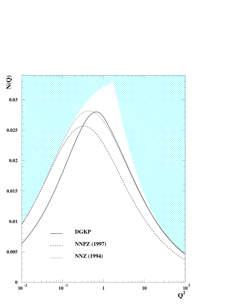
Figure 5: Integrated dipole distribution $N(Q)$ as a function of $Q^{2}$. The curves corresponding to the different models for the meson wave function are shown. The shaded area is theoretically forbidden.

References

- [1] K. Golec-Biernat, M. Wüsthoff, Phys. Rev. D59 (1999) 014017; Phys. Rev. D60 (1999) 114023.
- [2] U. Amaldi, K.R. Schubert, Nucl. Phys. B166 (1980) 301.
- [3] N.N. Nikolaev and B.G. Zakharov, Z. Phys. C49 (1991) 607; Z. Phys C53 (1992) 331; Z. Phys. C64 (1994) 651; JETP 78 (1994) 598.
- [4] A. H. Mueller, Nucl. Phys. B415 (1994) 373; A. H. Mueller and B. Patel, Nucl. Phys. B425 (1994) 471; A. H. Mueller, Nucl. Phys. B437 (1995) 107.
- [5] J. D. Bjorken, J. B. Kogut and D. E. Soper, Phys. Rev. D3 (1971) 1382.
- [6] A.H. Mueller, Eur. Phys. J. A1 (1998) 19.
- [7] L.D. Landau, E.M. Lifshitz, Quantum Mechanics, Mir, 1966.
-
[8]
H.G. Dosch, T. Gousset, G. Kulzinger and H.J. Pirner,
Phys. Rev. D55 (1997) 2602.
G. Kulzinger, H. G. Dosch and H. J. Pirner, Eur. Phys. J. C7 (1999) 73. - [9] J. Nemchik, N.N. Nikolaev, B.G. Zakharov , Phys.Lett. B341 (1994) 228.
- [10] J. Nemchik, N.N. Nikolaev, E. Predazzi, B.G. Zakharov, Z.Phys. C75 (1997) 71.
- [11] M. McDermott, L. Frankfurt, V. Guzey, M. Strikman, Eur. Phys. J. C16 (2000) 641.
- [12] M. Rueter, H.G. Dosch, Phys. Rev. D57 (1998) 4097.
- [13] J .R. Forshaw, G. Kerley, G. Shaw, Phys. Rev. D60 (1999) 074012.
- [14] G. Cvetic , D. Schildknecht, A. Shoshi, Acta Phys. Polon. B30 (1999) 3265.
- [15] A. Capella, E.G. Ferreiro, C.A. Salgado, A.B. Kaidalov, Nucl. Phys. B593 (2001) 336; Phys. Rev. D63 (2001) 054010.
- [16] S.J. Brodsky, L. Frankfurt, J.F. Gunion, A.H. Mueller, M. Strikman,Phys. Rev. D50 (1994) 3134.
- [17] L. Frankfurt, W. Koepf, M. Strikman, Phys. Rev. D54 (1996) 3194.
- [18] A. Caldwell and M.S. Soares, hep-ph/0101085.
- [19] ZEUS collaboration, Eur. Phys. J. C6 (1999) 603.
- [20] H1 collaboration Eur. Phys. J. C13 (2000) 371.
- [21] ZEUS collaboration, Study of the diffractive production of vector mesons at large or at large at HERA, EPS 1999, Tampere.
- [22] D.Yu. Ivanov, Phys. Rev. D53 (1996) 3564; I.F. Ginzburg, D.Yu. Ivanov, Phys. Rev. D54 (1996) 5523.
- [23] A.H. Mueller, Lectures given at International Summer School on Particle Production Spanning MeV and TeV Energies (Nijmegen 99), Nijmegen, Netherlands, 8-20 Aug 1999, and at MEETING-NOTE = 17th Autumn School: QCD: Perturbative or Nonperturbative? (AUTUMN 99), Lisbon, Portugal, 29 Sep - 4 Oct 1999. hep-ph/9911289.
- [24] A.H. Mueller, Nucl. Phys. B335 (1990) 115.
- [25] A.L. Ayala Filho, M.B. Gay Ducati, E.M. Levin, Nucl. Phys. B493 (1997) 305; Nucl. Phys. B511 (1998) 355.