ZU-TH 7/01

Dispersion relations and soft pion theorems for $K\to\pi\pi$

M. Büchler, G. Colangelo, J. Kambor and F. Orellana

Institute for Theoretical Physics, University of Zürich

Winterthurerstr. 190, CH-8057 Zürich, Switzerland

February 2001

We propose a new method to obtain the $K\to\pi\pi$ amplitude from $K\to\pi$ which allows one to fully account for the effects of final state interactions. The method is based on a set of dispersion relations for the $K\to\pi\pi$ amplitude in which the weak Hamiltonian carries momentum. The soft pion theorem, which relates this amplitude to the $K\to\pi$ amplitude, can be used to determine one of the two subtraction constants – the second constant is at present known only to leading order in chiral perturbation theory. We solve the dispersion relations numerically and express the result in terms of the unknown higher order corrections to this subtraction constant.

1. The $K\rightarrow\pi\pi$ amplitude has been the subject of numerous studies over the years, the main challenge being either to explain the $\Delta I=1/2$ rule or to provide a reliable estimate of $\varepsilon^{\prime}/\varepsilon$ [1, 2]. Among these attempts, the lattice approach is in principle the most rigorous as the weak matrix elements are calculated from first principles in a truly nonperturbative way. However, the inclusion of final state interactions is problematic. The calculation of the $K\rightarrow\pi\pi$ amplitude, e.g., proceeds by calculating the $K\rightarrow\pi$ amplitude on the lattice and using chiral perturbation theory (CHPT) at tree level to obtain the physical decay amplitude [3]. As is well known, the latter step induces a sizable uncertainty in the final result, commonly estimated to be around 30%, the typical size of next–to–leading order corrections in chiral SU(3). To discuss the relation between the $K\to\pi\pi$ and the $K\to\pi$ amplitude, it is necessary to allow the weak Hamiltonian to carry momentum. Then the former amplitude becomes a function of the usual three Mandelstam variables $s,\;t$ and $u$, and is identified with the physical decay amplitude at the point $s=M_{K}^{2}$, $t=u=M_{\pi}^{2}$. At the so–called soft–pion point (SPP), where the momentum of one of the two pions is sent to zero ($s=u=M_{\pi}^{2}$, $t=M_{K}^{2}$), this amplitude is related to the $K\to\pi$ amplitude, up to ${\cal O}(M_{\pi}^{2})$ corrections. The problem is how to extrapolate the amplitude from the SPP to the physical point. The only working method proposed so far has been to use CHPT at tree level [3] – using the one-loop relation does not solve the problem because a number of unknown low energy constants appear [4].

In the present letter we set up a dispersive framework for the $K\to\pi\pi$ amplitude. We show that by solving numerically the dispersion relations one can do the extrapolation in a controlled manner. The unitarity corrections due to rescattering of the pions in the final state, and those due to $\pi K$ (virtual) rescattering in the $t$ and $u$ channels, can be accurately accounted for by solving the dispersion relations. These effects, which also appear to one loop in CHPT, are not the only source of possible large corrections to tree level: two subtraction constants appear which may also suffer from large ${\cal O}(M_{K}^{2})$ corrections. The soft–pion theorem provides the means to determine one of the two subtraction constants, up to terms of order $M_{\pi}^{2}$. The other constant (the derivative in $s$ of the amplitude at the SPP) is unfortunately not yet determined with the same accuracy, and at present can be estimated only with tree-level CHPT. A better determination of this constant is the core of the problem. Once solved the $K\to\pi\pi$ amplitude can be obtained with substantially smaller uncertainties than at present.

Truong [5], and more recently Pallante and Pich [6], have stressed the importance of final state interactions in $K\to\pi\pi$, for the $\Delta I=1/2$ rule and $\varepsilon^{\prime}/\varepsilon$, respectively. In estimating these effects they rely on the dispersion relation for the $K\to\pi\pi$ amplitude with the kaon off-shell. While the method provides a quick and simple estimate of the effect of final state interactions, it is not trivial to promote it to a systematic and rigorous calculation. The problems related to the formulation and the use of dispersion relations for an off-shell amplitude are discussed in a separate note [7] (see also [8]).

2. We consider the amplitude

$$\langle\pi(p_{1})\pi(p_{2})(I=0)|{\cal H}^{1/2}_{W}(0)|K(q_{1})\rangle=:T^{+}(s,t,u)$$ (1)

described in terms of the Mandelstam variables:

$$s=(p_{1}+p_{2})^{2},\;\;t=(q_{1}-p_{1})^{2},\;\;u=(q_{1}-p_{2})^{2}\;\;,$$ (2)

related by $s+t+u=2M_{\pi}^{2}+M_{K}^{2}+q_{2}^{2}$, where $q_{2}$ is the momentum carried by the weak Hamiltonian. From now on we set $q_{2}^{2}=0$ (but $q_{2}^{\mu}\neq 0$ in general). The physical decay amplitude is obtained by setting $q_{2}^{\mu}=0$ ($s=M_{K}^{2}$, $t=u=M_{\pi}^{2}$).

Since the weak Hamiltonian has the quantum numbers of the kaon, and the pions are in an isospin zero state, the amplitude (1) is analogous to the $t\leftrightarrow u$ even combination of the $KK\to\pi\pi$ scattering amplitude (the notation is borrowed from Ref. [9]). Like in that case, one can show that if one neglects the imaginary parts of $D$ waves and higher in all channels, then the analytic structure of the amplitude simplifies and it can be decomposed into a combination of functions of a single variable (for the $K\pi$ scattering case see [10]):

$$T^{+}(s,t,u) = M_{0}(s)+{1\over 3}\left[N_{0}(t)+N_{0}(u)\right]+{2\over 3}\left[R_{0}(t)+R_{0}(u)\right]$$ (3)

$$+ {1\over 2}\left[\left(s-u-{M_{\pi}^{2}\Delta\over t}\right)N_{1}(t)+\left(s-t-{M_{\pi}^{2}\Delta\over u}\right)N_{1}(u)\right]\;\;,$$

where $\Delta=M_{K}^{2}-M_{\pi}^{2}$. Notice that the terms proportional to $N_{1}$ drop out from the physical decay amplitude:

$${\cal A}(K\to\pi\pi) = T^{+}(M_{K}^{2},M_{\pi}^{2},M_{\pi}^{2})=$$ (4)

$$= M_{0}(M_{K}^{2})+{2\over 3}\left[N_{0}(M_{\pi}^{2})+2R_{0}(M_{\pi}^{2})\right]\;\;.$$

Each of the single variable functions appearing in Eq. (3) is analytic in the complex plane except for a cut starting at $4M_{\pi}^{2}$ for $M_{0}$ and at $(M_{K}+M_{\pi})^{2}$ for the remaining ones. These functions are defined to have the discontinuity on the positive real axis identical to that of a specific partial wave: $M_{0}$ to the $I=0$ $S$-wave in the $s$ channel, whereas in the $t$ channel, $N_{0}$ and $N_{1}$ to the $I=1/2$ $S$- and $P$- wave respectively, and $R_{0}$ to the $I=3/2$ $S$-wave. Below the inelastic threshold, the elastic unitarity condition for these functions reads

$${\rm disc}M_{0}(s) = \sin\delta_{0}^{0}(s)e^{-i\delta_{0}^{0}}\left[M_{0}(s)+\hat{M}_{0}(s)\right]\;\;,$$

$${\rm disc}N_{\ell}(s) = \sin\delta_{\ell}^{1/2}(s)e^{-i\delta_{\ell}^{1/2}}\left[N_{\ell}(s)+\hat{N}_{\ell}(s)\right]\;\;,$$

$${\rm disc}R_{0}(s) = \sin\delta_{0}^{3/2}(s)e^{-i\delta_{0}^{3/2}}\left[R_{0}(s)+\hat{R}_{0}(s)\right]\;\;,$$ (5)

where $\delta_{0}^{0}$ is the $\pi\pi$ phase shift, whereas those with half-integer isospin are the $\pi K$ phase shifts.

The hat functions denote contributions from the other channels coming in via angular averages (to be specified below), and are defined as

$$\hat{M}_{0}(s) = \left[s\Sigma_{1}-2M_{K}^{2}M_{\pi}^{2}-{1\over 4}(M_{K}^{4}+3s^{2})\right]\langle\tilde{N}_{1}\rangle+2s|\mathbf{p}||\mathbf{q}|\langle z\tilde{N}_{1}\rangle$$

$$+ 4|\mathbf{p}|^{2}|\mathbf{q}|^{2}\langle z^{2}\tilde{N}_{1}\rangle+{2\over 3}(\langle N_{0}\rangle+2\langle R_{0}\rangle)\;\;,$$

$$\hat{N}_{0}(t) = \langle M_{0}\rangle_{s}+y(t)\langle M_{1}\rangle_{s}-r(t)\langle zM_{1}\rangle_{s}+{1\over 3}\left(4\langle R_{0}\rangle_{u}-\langle N_{0}\rangle_{u}\right)$$

$$- {1\over 8}w(t)\langle\tilde{N}_{1}\rangle_{u}-{1\over 4}v(t)\langle z\tilde{N}_{1}\rangle_{u}+{1\over 8}r^{2}(t)\langle z^{2}\tilde{N}_{1}\rangle_{u}\;\;,$$

$$\hat{N}_{1}(t) = {2\over r(t)}\left\{\langle zM_{0}\rangle_{s}+y(t)\langle zM_{1}\rangle_{s}-r(t)\langle z^{2}M_{1}\rangle_{s}+{1\over 3}\left(4\langle zR_{0}\rangle_{u}-\langle zN_{0}\rangle_{u}\right)\right.$$

$$- \left.{1\over 8}w(t)\langle z\tilde{N}_{1}\rangle_{u}-{1\over 4}v(t)\langle z^{2}\tilde{N}_{1}\rangle_{u}+{1\over 8}r^{2}(t)\langle z^{3}\tilde{N}_{1}\rangle_{u}\right\}$$

$$\hat{R}_{0}(t) = \langle M_{0}\rangle_{s}-{1\over 2}y(t)\langle M_{1}\rangle_{s}+{1\over 2}r(t)\langle zM_{1}\rangle_{s}+{1\over 3}\left(\langle R_{0}\rangle_{u}+2\langle N_{0}\rangle_{u}\right)\;\;,$$ (6)

$$+ {1\over 4}w(t)\langle\tilde{N}_{1}\rangle_{u}+{1\over 2}v(t)\langle z\tilde{N}_{1}\rangle_{u}\!-\!{1\over 4}r^{2}(t)\langle z^{2}\tilde{N}_{1}\rangle_{u}\;\;,$$

where

$$\tilde{N}_{1}(t)\!\! \!\!=\!\! \!\!N_{1}(t)/t\;,\;\;\Sigma=M_{K}^{2}+M_{\pi}^{2}\;,\;\;\Sigma_{1}=\Sigma+M_{\pi}^{2}\;,\;\;y(t)=\Sigma_{1}-3t-{M_{\pi}^{2}\Delta\over t}\;\;,$$

$$\rho_{\pi K}(t)\!\! \!\!=\!\! \!\!\sqrt{\left(1-(M_{K}\!+\!M_{\pi})^{2}/t\right)\left(1-(M_{K}\!-\!M_{\pi})^{2}/t\right)}\;\;,\;\;r(t)=(t-M_{\pi}^{2})\rho_{\pi K}(t)\;\;,$$

$$v(t)\!\! \!\!=\!\! \!\!\left(t-{M_{\pi}^{2}\Delta\over t}\right)r(t)\;\;,\;\;\;\;w(t)=3t^{2}-4t\Sigma_{1}+5M_{\pi}^{4}+\Sigma^{2}-{M_{\pi}^{4}\Delta^{2}\over t^{2}}\;\;.$$ (7)

The brackets $\langle\rangle$ indicate angular averages defined as

$$\langle z^{n}X\rangle(s)\!\! \!\!=\!\! \!\!{1\over 2}\int_{-1}^{1}dzz^{n}X(\Sigma_{1}/2-s/2+2|\mathbf{p}||\mathbf{q}|z)$$

$$\langle z^{n}X\rangle_{v}(t)\!\! \!\!=\!\! \!\!{1\over 2}\int_{-1}^{1}dzz^{n}X(v(t,z))\;\;\;\;\;\;v=s,u\;\;,$$ (8)

where

$${|\mathbf{p}|}^{2}={s\over 4}-M_{\pi}^{2},\;{|\mathbf{q}|}^{2}={s\over 4}\left(1-{M_{K}^{2}\over s}\right)^{2};\;s+u=\Sigma_{1}-t,\;s-u={M_{\pi}^{2}\Delta\over t}+r(t)z\;.$$ (9)

In the definition of the hat functions the function $M_{1}$ appears. This is analogous to $M_{0}$, in the case of the $I=1$ $P$-wave in the $s$ channel, and is necessary to describe the process (1) in full generality, for all channels (including the $t\leftrightarrow u$ odd, $I=1$ $s$–channel). It does not contribute directly to the physical decay process: its indirect (and small) contribution via the angular average in the dispersion relation is a consequence of crossing symmetry.

3. If one is only interested in the low–energy region, neglecting the inelastic channels is a good approximation: then the solution of the dispersion relation for each of the functions is well approximated by the Omnès function times a polynomial [11]. It is therefore convenient to write the dispersion relation for the functions divided by the corresponding Omnès function (see [12] for a detailed discussion of this point, although in a different framework), in the following form:

$$M_{0}(s) = \Omega_{0}^{0}(s,s_{0})\left\{a+b(s\!-\!s_{0})+{(s\!-\!s_{0})^{2}\over\pi}\int_{4M_{\pi}^{2}}^{\Lambda_{1}^{2}}{\sin\delta_{0}^{0}(s^{\prime})\hat{M}_{0}(s^{\prime})ds^{\prime}\over|\Omega_{0}^{0}(s^{\prime},s_{0})|(s^{\prime}\!-\!s)(s^{\prime}\!-\!s_{0})^{2}}\right\}$$

$$N_{0}(s) = \Omega_{0}^{1/2}(s)\left\{{s^{2}\over\pi}\int_{(M_{K}+M_{\pi})^{2}}^{\Lambda_{2}^{2}}{\sin\delta_{0}^{1/2}(s^{\prime})\hat{N}_{0}(s^{\prime})ds^{\prime}\over|\Omega_{0}^{1/2}(s^{\prime})|(s^{\prime}-s)s^{\prime 2}}\right\}$$

$$N_{1}(s) = \Omega_{1}^{1/2}(s)\left\{{s\over\pi}\int_{(M_{K}+M_{\pi})^{2}}^{\Lambda_{2}^{2}}{\sin\delta_{1}^{1/2}(s^{\prime})\hat{N}_{1}(s^{\prime})ds^{\prime}\over|\Omega_{1}^{1/2}(s^{\prime})|(s^{\prime}-s)s^{\prime}}\right\}$$

$$R_{0}(s) = \Omega_{0}^{3/2}(s)\left\{{s^{2}\over\pi}\int_{(M_{K}+M_{\pi})^{2}}^{\Lambda_{2}^{2}}{\sin\delta_{0}^{3/2}(s^{\prime})\hat{R}_{0}(s^{\prime})ds^{\prime}\over|\Omega_{0}^{3/2}(s^{\prime})|(s^{\prime}-s)s^{\prime 2}}\right\}\;\;.$$ (10)

$\Omega^{I}_{\ell}(s)$ is the Omnès function [11], defined as

$$\Omega^{0}_{0}(s,s_{0}) = \exp\left\{{(s-s_{0})\over\pi}\int_{4M_{\pi}^{2}}^{\tilde{\Lambda}_{1}^{2}}ds^{\prime}{\delta^{0}_{0}(s^{\prime})\over(s^{\prime}-s_{0})(s^{\prime}-s)}\right\}\;\;$$

$$\Omega^{I}_{\ell}(s) = \exp\left\{{s\over\pi}\int_{(M_{K}+M_{\pi})^{2}}^{\tilde{\Lambda}_{2}^{2}}ds^{\prime}{\delta^{I}_{\ell}(s^{\prime})\over s^{\prime}(s^{\prime}-s)}\right\}~{}~{}~{}~{}~{}~{}~{}~{}~{}~{}~{}~{}~{}~{}I={1\over 2},{3\over 2}\;\;.$$ (11)

All functions are subtracted at $s=0$ with the only exception of $M_{0}$, where the subtraction point $s_{0}$ is left unspecified. In the following we use $s_{0}=M_{\pi}^{2}$. The fact that only $M_{0}$ depends on subtraction constants does not have any deep reason: the splitting of polynomial terms of $T^{+}$ between the various functions $M_{0}$, $N_{0,1}$ and $R_{0}$ is arbitrary, and we have merely used this freedom to remove them from the latter three. The final result does not depend on this choice [12]. All the dispersive integrals above have been cut off at energies $\Lambda_{1,2}$ and $\tilde{\Lambda}_{1,2}$ – numerical values will be given below.

4. If the $\pi\pi$ and $K\pi$ phase shifts, the cutoffs $\Lambda_{1,2}$, and the subtraction constants $a$ and $b$ are given, the dispersion relations (10) can be solved numerically. Such a solution gives the amplitude $T^{+}(s,t,u)$ at any point (provided it is far enough from the inelastic thresholds) of the Mandelstam plane, in particular at the physical point. The crucial new inputs here are the two subtraction constants: the phase shifts are known with sufficient accuracy, whereas the choice of the cutoffs is dictated by the inelastic thresholds. Before proceeding, we have to discuss how these two subtraction constants can be determined. If they could be calculated with better accuracy than the physical amplitude itself, then this would represent for our method a clear advantage.

For one of the two subtraction constants this is the case. The soft–pion theorem relates the amplitude at the SPP to the $K\to\pi$ amplitude up to terms of order $M_{\pi}^{2}$. We can therefore write

$$-{1\over 2F_{\pi}}{\cal A}(K\to\pi)=a+{1\over 3}\left[N_{0}(M_{K}^{2})+2R_{0}(M_{K}^{2})\right]+{\cal O}(M_{\pi}^{2})\;\;,$$ (12)

which shows that $a$ is indeed directly related to a quantity that is calculable (more easily than the decay amplitude itself), e.g. on the lattice. The relation (12) illustrates the strength of the soft–pion theorem: although the process involves a kaon, the relation is based on the use of the $SU(2)$ symmetry, and therefore suffers from corrections of order $M_{\pi}^{2}$ only.

The key of the problem is how to calculate $b$. This constant is related to the derivative in $s$ of the amplitude $T^{+}$ at the SPP. The calculation of $b$ requires the evaluation of the physical amplitude $T^{+}$ at an unphysical point, via analytic continuation. While this is easy to do with an analytical method like CHPT, it is practically impossible with a numerical method, like the lattice. However there is a Ward identity that relates this derivative to a Green function that is directly calculable:

$${\partial\over\partial s}T^{+}(s,\Sigma-s,M_{\pi}^{2})_{|s=M_{\pi}^{2}}={1\over 2}C(M_{\pi}^{2},M_{K}^{2},M_{\pi}^{2})+{\cal O}(M_{\pi}^{2})\;\;,$$ (13)

where $C(s,t,u)$ is an amplitude defined as:

$${i\over F_{\pi}}\int\!\!dxe^{ip_{1}x}\langle\pi(p_{2})|T{\cal H}_{W}^{1/2}(0)A^{\mu}(x)|K(q_{1})\rangle=ip_{1}^{\mu}B+iq_{1}^{\mu}C+iq_{2}^{\mu}D\;,$$ (14)

where $A^{\mu}(x)$ is the axial current that couples to the pion removed from the outgoing state. By making the $p_{2}$ momentum soft one can also derive a soft-pion theorem which relates the four-point function in Eq. (14) to a three-point function. Unfortunately the function $C$ cannot be singled out from this relation.

We are not aware of any attempts to calculate $b$. In order to illustrate our method we proceed by fixing $b$ at a certain value and then varying it within a fairly wide range. To fix the central value and the range we use CHPT as a guide. At leading order, CHPT dictates the following relation between $a$ and $b$:

$$b={3a\over M_{K}^{2}-M_{\pi}^{2}}\left(1+X+{\cal O}(M_{K}^{4})\right)\;\;.$$ (15)

The size of the correction is at the moment unknown, but nothing protects it from being of order $M_{K}^{2}$: $X=M_{K}^{2}/(16\pi^{2}F_{K}^{2})x$, with $x$ expected to be of order one. An explicit calculation in CHPT yields [13]:

$$x\! \!=\! \!\frac{383}{9}-\frac{8021}{54}\ln{4\over 3}+\frac{1}{3}\ln{M_{K}^{2}\over M_{\pi}^{2}}-\frac{8}{3}(\bar{N}_{5}+2\bar{N}_{7}-\bar{N}_{9}-4\bar{N}_{10}-4\bar{N}_{11})$$ (16)

$$+ 2(\bar{N}_{19}-\bar{N}_{20})-\frac{4}{3}(2\bar{N}_{21}+\bar{N}_{22}+2\bar{N}_{23})+{\cal O}\left({M_{\pi}^{2}\over M_{K}^{2}}\right)\;,$$

where $\bar{N}_{i}=16\pi^{2}N_{i}^{r}(M_{K})$ are the renormalized low-energy constants introduced in [14]. Since we lack information on many of the constants, the CHPT calculation (16) does not allow us to do more than an order of magnitude estimate for $b$.

5.

Figure 1: The function $|T^{+}(s,t,u)|$ plotted vs. $E=\sqrt{s}$ along the line of constant $u=M_{\pi}^{2}$: the result of our numerical study for different values of $X$ are compared to tree level CHPT.

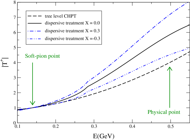
In our numerical study we have used $X=\pm 30\%$. The normalization of the amplitude is irrelevant here, and we have fixed it to $T^{+}(M_{\pi}^{2},M_{K}^{2},M_{\pi}^{2})=1$. The $\pi\pi$ phase shifts are taken from [15], with the scattering lengths determined in [16], and the $\pi K$ phase shifts from [17]. For the cutoffs we have used $\Lambda_{1}=1$ GeV, $\Lambda_{2}=1.3$ GeV, and $\tilde{\Lambda}_{i}=1.05\Lambda_{i}$. Our results are shown in Fig. 1, where we have plotted $|T^{+}(s,\Sigma-s,M_{\pi}^{2})|$ versus $s$, comparing our numerical solution of the dispersion relations to the CHPT leading order formula. The latter is what has been used so far whenever a number for the $K\to\pi\pi$ matrix element extracted from the lattice has been given. Our treatment shows that large corrections with respect to leading–order CHPT are to be expected. One source of large corrections is the Omnès factor due to $\pi\pi$ rescattering in the final state [6, 5]. The other potentially dangerous source is represented by $X$, the next-to-leading order correction to the relation (15) between $a$ and $b$. The latter could (depending on the sign) in principle double, or to a large extent reabsorb the correction due to final state interactions. The dependence on $X$ is well described by the following linear formula:

$${|{\cal A}(K\to\pi\pi)|\over|{\cal A}^{\mbox{\tiny LO CHPT}}(K\to\pi\pi)|}=1.5\left(1+0.76X\right)\;\;,$$ (17)

after having normalized both amplitudes to $T^{+}(M_{\pi}^{2},M_{K}^{2},M_{\pi}^{2})=1$. The evaluation of the uncertainties to be attached to the numbers in Eq. (17) is in progress [18]. At the moment, however, the main source of uncertainty is the fact that $X$ is largely unknown.

One of the outcomes of the present analysis is that the effects embodied in the functions $N_{0,1}$ and $R_{0}$ have turned out to be very small: if we drop them altogether, the numbers in Eq. (17) change from 1.5 to 1.4 and from 0.76 to 0.75. Notice that these effects are in principle of order $M_{K}^{2}$, as can be seen in Eq. (12), and that they are not a priori negligible. On the other hand this result is very much welcome, because the size of these functions depends both on the $\pi K$ phases (which are less well known than the $\pi\pi$ ones) and on the choice of the cutoff $\Lambda_{2}$, which may induce large uncertainties.

6. The authors of [3] have given a recipe to remove by hand the contribution of the weak mass term to the $K\to\pi$ transition. This step is necessary since at tree level the weak mass term does not contribute to the $K\to\pi\pi$ amplitude. The procedure suggested in [3] involved the calculation of the $K\to$ vacuum transition. In our framework this procedure is unnecessary. To show this it is useful to work with the tree-level CHPT amplitude (weak mass contribution only, see [14] for the notation):

$$T^{+}_{c_{5}}(s,t,u)=\frac{-ic_{5}\Delta}{F_{\pi}^{2}}\left[\frac{s}{q_{2}^{2}-M_{K}^{2}}+1\right]\;\;,$$ (18)

where we have restored $q_{2}^{2}\neq 0$ to show explicitly the presence of the kaon pole. At the physical point this amplitude vanishes. On the other hand, if we calculate this amplitude at the SPP, from the corresponding $K\to\pi$ amplitude, we cannot get the kaon-pole term, and therefore would obtain a nonvanishing contribution at the physical point. Hence the cure proposed in [3]. The fact that the $K\to\pi$ amplitude does not contain the pole term does not contradict the soft-pion theorem: at the SPP, for $q_{2}^{2}=0$, the pole term is of order $M_{\pi}^{2}$, which is beyond the accuracy the theorem guarantees.

The framework proposed here relies on the presence of two subtraction constants, that we have related to the amplitude and its derivative at the SPP. If one determines both constants at tree level in CHPT (18), one finds that the subtraction polynomial vanishes at the physical point, without further ado. This cancellation does not happen if the subtraction constants are given to one loop – but it does not need to: as is well known [4], the $K\to\pi\pi$ amplitude does contain contributions proportional to $c_{5}$ at one loop.

7. In the present paper we have set up a dispersive framework for the $K\rightarrow\pi\pi$ amplitude that allows one to evolve the amplitude from the soft-pion point (where it is given by the $K\rightarrow\pi$ amplitude) to the physical point, taking into account all the main physical effects. As we have pointed out, this evolution is on safe ground only if a second input is made available: the derivative of the amplitude at the soft-pion point which, to the best of our knowledge, has not been calculated so far. We have calculated this second subtraction constant to next-to-leading order in CHPT. Given the presence of unknown low-energy constants, we cannot use this expression for more than an order of magnitude estimate. Our numerical work, however, shows that the amplitude at the physical point depends strongly on the value of the slope at the SPP, see Fig. 1 and related discussion in the text. A nonperturbative calculation of the second subtraction constant $b$ is necessary in order to obtain an accurate result with this method. We have provided a Ward identity which might be useful in this respect.

Lattice calculations of the $K\rightarrow\pi\pi$ amplitude made so far [2] rely on tree-level CHPT to relate the calculated $K\rightarrow\pi$ matrix elements to the physical decay amplitude. The method proposed here improves this scheme by combining input from the lattice with dispersive techniques, thereby providing a fully consistent treatment of final state interactions in $K\rightarrow\pi\pi$. Given the two subtraction constants, the dispersion relations can be solved numerically to good accuracy. Recently, a direct calculation of the $K\to\pi\pi$ matrix element on the lattice has been proposed in Ref. [19] – this method does not rely on CHPT. Other lattice methods, which also do not rely on the evaluation of the $K\to\pi$ amplitude had also been proposed previously [20]. Each of these methods presents different technical problems in its practical implementation [21], and it is difficult to predict which one will lead to a reliable calculation of the $K\to\pi\pi$ amplitude. We hope that the present work will stimulate further efforts to calculate the subtraction constants $a$ and $b$, either on the lattice, or by other nonperturbative methods.

Acknowledgements   It is a pleasure to thank J. Gasser, G. Isidori, E. Pallante, T. Pich, and D. Wyler for interesting discussions. This work was supported by the Schweizerische Nationalfonds, by TMR, BBW-Contract No. 97.0131 and EC-Contract No. ERBFMRX-CT980169 (EURODA$\Phi$NE).