[

VUTH 01-03 The Collins fragmentation function: a simple model calculation

Abstract

The Collins function belongs to the class of the so-called time-reversal odd fragmentation functions. Being chiral-odd as well, it can serve as an important tool to observe the nucleon’s transversity distribution in semi-inclusive DIS. Due to the possible presence of final state interactions, this function can be non-zero, though this has never been demonstrated in an explicit model calculation. We use a simple pseudoscalar coupling between pions and quarks to model the fragmentation process and we show that the inclusion of one-loop corrections generates a non-vanishing Collins function, therefore giving support to its existence from the theoretical point of view.

]

Our understanding of hadronic physics depends strongly on what we know about the parton distribution and fragmentation functions, which are universal, process-independent objects. While in the past several experiments provided us with considerable information on the parton distributions, our knowledge of the fragmentation functions is still rather limited.

A lot of attention has been devoted to the class of the so-called time-reversal odd (T-odd) fragmentation functions, among which the Collins function $H_{1}^{\perp}$ [1, 2] is the most prominent example. In contrast to a naive expectation, these functions can be non-vanishing because time-reversal invariance does not impose any constraint [1, 3] (in the literature they are sometimes referred to as naive T-odd functions [4]). This is a consequence of possible final state interactions in the fragmentation process, giving rise to a non-trivial phase (imaginary part) [1]. We remark that final state interactions should not be considered exclusively as reinteractions of the outgoing hadron with the rest of the jet, as we will discuss in more detail later.

The Collins function describes the fragmentation of a transversely polarized quark into an unpolarized hadron (e.g. a pion), i.e. the process $q^{\ast}\to hX$. The introduction of this function requires taking into account the quark’s transverse momentum. Although the Collins function in itself deserves attention towards understanding the physics governing the fragmentation process, it is particularly relevant because in semi-inclusive DIS it can serve as the chiral-odd partner needed to access the transversity distribution of the nucleon, $h_{1}$, which is chiral-odd as well. The transversity is a crucial property of the nucleon, carrying information on its spin structure complementary to what we can deduce from helicity distributions. Because of its chiral-odd nature, $h_{1}$ is suppressed in inclusive DIS, and therefore it has remained essentially unexplored on the experimental side. In the case of one-particle inclusive DIS, where one detects only a single hadron in the final state, the Collins function provides the only possibility to probe $h_{1}$ at the leading twist level.

Even if the Collins function can not be discarded in general on the basis of time-reversal invariance, it has been suspected to vanish since the effect arising from final state interactions may average out [5]. Moreover, $H_{1}^{\perp}$ has been proven elusive to previous modeling attempts [4]. This suggested to turn the attention to the experimentally more challenging detection of two hadrons in a semi-inclusive measurement [6, 5], as an alternative method to measure the transversity. Until now, no ab initio calculation has ever displayed the possibility of generating a non-zero Collins function in the framework of a simple, time-reversal invariant model.

On the experimental side, the HERMES collaboration reported the first observation of a single-spin asymmetry in semi-inclusive pion production [7], which could be interpreted as arising from the contribution of the Collins function [8]. Analogously, large single-spin asymmetries in the process $p^{\uparrow}p\rightarrow\pi X$ [9] could also be explained by means of the Collins function [10]. The situation is far from clear, but further investigations are among the priorities of the HERMES [11], COMPASS [12] and possibly eRHIC programs.

In these circumstances, producing a non-zero Collins function in a simple yet consistent model is an interesting and relevant result, which we are going to present in this letter. To this end we describe the fragmentation process by a pseudoscalar coupling between quarks and pions in the one-loop approximation. A similar calculation has been suggested earlier [13], but never carried out explicitly. For what concerns possible phenomenological applications, we do not pretend our calculation to be realistic, but we think that it can shed light on the identity of T-odd fragmentation functions and can conclusively affirm that there are no theoretical reasons to believe the Collins function to vanish.

Considering the fragmentation process $q^{\ast}(k)\to\pi(p)X$, we define the Collins function, which depends on the longitudinal momentum fraction $z$ of the pion and the transverse momentum $k_{{\scriptscriptstyle T}}$ of the quark, as [14]

$$\frac{\epsilon_{{\scriptscriptstyle T}}^{ij}k_{{\scriptscriptstyle T}\,j}}{m_{\pi}}\,H_{1}^{\perp}(z,k^{2}_{{\scriptscriptstyle T}})=\left.\frac{1}{4z}\int{\rm\,d}k^{+}\;\mbox{Tr}\,[\Delta(k,p){\rm i}\sigma^{i-}\gamma_{5}]\right|_{k^{-}=\frac{p^{-}}{z}},$$ (1)

with $m_{\pi}$ denoting the pion mass and $\epsilon_{{\scriptscriptstyle T}}^{ij}\equiv\epsilon^{ij-+}$ (we specify the plus and minus lightcone components of a generic 4-vector $a^{\mu}$ according to $a^{\pm}\equiv(a^{0}\pm a^{3})/\sqrt{2}$). The correlation function $\Delta(k,p)$ in Eq. (1), omitting gauge links, takes the form

$$\Delta(k,p)=\sum_{X}\,\int\frac{{\rm\,d}^{4}\xi}{(2\pi)^{4}}{\rm e}^{+{\rm i}k\cdot\xi}\langle 0|\,\psi(\xi)|\pi,X\rangle\langle\pi,X|\overline{\psi}(0)|0\rangle.$$ (2)

To describe the matrix elements in the correlation function, we use a pseudoscalar coupling between quarks and pions given by the interaction Lagrangian

$${\cal L}_{I}(x)={\rm i}g\,\overline{q}(x)\gamma_{5}q(x)\pi(x)\,,$$ (3)

which is in the spirit of the Manohar–Georgi model [15]. This is clearly an oversimplified approach to the fragmentation $q^{\ast}\to\pi X$ but the model contains the essential elements required for our discussion. In particular, it is time-reversal invariant. One could also perform the calculation in a chirally invariant model by including a scalar $\sigma$ field as well as taking quark flavors properly into account. In our view, this is certainly necessary to improve the result obtained here for a better description of the phenomenology, but the essential result of a non-zero $H_{1}^{\perp}$ is already evident without going to the complications arising from the inclusion of the $\sigma$ particle and the discussion of various flavors.

Using the Lagrangian in Eq. (3), at tree level the fragmentation of a quark is modeled through the process $q^{\ast}\to\pi q$. The corresponding correlation function can be represented by the unitarity diagram in Fig. 1 and reads explicitly

$$\Delta_{(0)}(k,p) = -\frac{g^{2}}{(2\pi)^{4}}\,\frac{(\hbox to0.0pt{/\hss}k+m)}{k^{2}-m^{2}}\,\gamma_{5}\,(\hbox to0.0pt{/\hss}k-\hbox to0.0pt{/\hss}p+m)\,\gamma_{5}\,\frac{(\hbox to0.0pt{/\hss}k+m)}{k^{2}-m^{2}}$$ (5)

$$\mbox{}\times 2\pi\,\delta((k-p)^{2}-m^{2})\,,$$

where $m$ represents the mass of a constituent quark. Using this correlation function, the unpolarized fragmentation function

$$D_{1}(z,k^{2}_{{\scriptscriptstyle T}})=\left.\frac{1}{4z}\int{\rm\,d}k^{+}\;\mbox{Tr}\,[\Delta(k,p)\gamma^{-}]\right|_{k^{-}=\frac{p^{-}}{z}}$$ (6)

in our model at tree level becomes

$$D_{1}(z,k^{2}_{{\scriptscriptstyle T}})=\frac{1}{z}\frac{g^{2}}{16\pi^{3}}\,\frac{k_{{\scriptscriptstyle T}}^{2}+m^{2}}{(k_{{\scriptscriptstyle T}}^{2}+m^{2}+\frac{1-z}{z^{2}}m_{\pi}^{2})^{2}}\,.$$ (7)

In the case of $m_{\pi}=0$ we recover the result already obtained by Collins [1]. Contrary to $D_{1}$, the Collins function at tree level is zero. This is not surprising because at tree level no final state interaction appears in the fragmentation process, which is supposed to be the origin of the T-odd fragmentation functions like $H_{1}^{\perp}$. The situation changes when we proceed to one-loop corrections, as we explicitly show in the following.

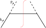
FIG. 1.: Lowest-order unitarity diagram describing the fragmentation of a quark into a pion.

A consistent one-loop calculation of the fragmentation process requires the evaluation of all the diagrams shown in Fig. 2. In the actual calculation only the asymmetric diagrams (a–d) contribute. The contributions from the diagrams (e), (g) and (h) vanish individually when projecting out the Collins function, while the contributions of diagram (f) and its hermitian conjugate cancel each other.

It should be noted that not all the asymmetric (interference-type) diagrams contribute. For example, the diagram (f) and its hermitian conjugate represent the interference between two different tree level amplitudes describing the process $q^{\ast}\rightarrow\pi\pi q$. However, their contributions to the Collins function cancel each other since the involved interfering amplitudes are purely real. In calculating $H_{1}^{\perp}$, such a cancellation between contributions coming from a diagram and its hermitian conjugate takes place whenever the involved amplitudes are purely real and is a model independent feature.

In our computation, the relevant components to be included are the self-energy correction for diagrams (a) and (b), and the vertex correction for diagrams (c) and (d). These corrections are sketched in Fig. 3 and can be analytically expressed as

$$-{\rm i}\Sigma(k) = -g^{2}\int\frac{{\rm\,d}^{4}l}{(2\pi)^{4}}\,\frac{\hbox to0.0pt{/\hss}l-\hbox to0.0pt{/\hss}k+m}{[(k-l)^{2}-m^{2}]\,[l^{2}-m_{\pi}^{2}]}\,,$$ (8)

$$g\gamma_{5}\Gamma(k,p) = -{\rm i}g^{3}\gamma_{5}\int\frac{{\rm\,d}^{4}l}{(2\pi)^{4}}\,\frac{(\hbox to0.0pt{/\hss}k-\hbox to0.0pt{/\hss}p-\hbox to0.0pt{/\hss}l+m)}{[(k-p-l)^{2}-m^{2}]}$$ (10)

$$\mbox{}\times\frac{(\hbox to0.0pt{/\hss}l-\hbox to0.0pt{/\hss}k+m)}{[(l-k)^{2}-m^{2}][l^{2}-m_{\pi}^{2}]}\,.$$

The functions $\Sigma(k)$ and $\Gamma(k,p)$ can be parametrized as

$$\Sigma(k) = A\,\hbox to0.0pt{/\hss}k+B\,m\,,$$ (11)

$$\Gamma(k,p) = C+D\,\hbox to0.0pt{/\hss}p+E\,\hbox to0.0pt{/\hss}k+F\,\hbox to0.0pt{/\hss}p\,\hbox to0.0pt{/\hss}k.$$ (12)

The real parts of the functions $A$, $B$, $C$ etc. are UV-divergent and require in principle a proper renormalization. Though our model is renormalizable, we do not have to deal with this question at all, since only the imaginary parts of the loop diagrams will turn out to be important.

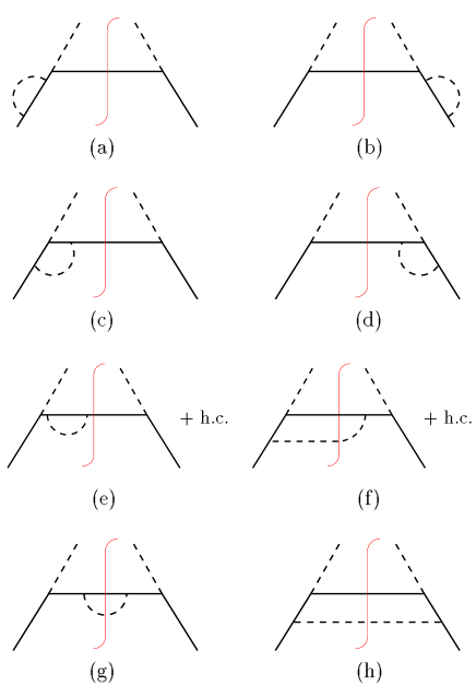
FIG. 2.: One-loop corrections to the fragmentation of a quark into a pion.

The contributions to the correlation function generated by the diagrams (a) and (c) are given by:

$$\Delta_{(1)}^{(a)}(k,p)=-\frac{g^{2}}{(2\pi)^{4}}\,\frac{(\hbox to0.0pt{/\hss}k+m)}{k^{2}-m^{2}}\,\gamma_{5}\,(\hbox to0.0pt{/\hss}k-\hbox to0.0pt{/\hss}p+m)\,\gamma_{5}$$ (14)

$$\quad\mbox{}\times\frac{(\hbox to0.0pt{/\hss}k+m)}{k^{2}-m^{2}}\,\Sigma(k)\,\frac{(\hbox to0.0pt{/\hss}k+m)}{k^{2}-m^{2}}\;2\pi\;\delta((k-p)^{2}-m^{2})\,,$$

$$\Delta_{(1)}^{(c)}(k,p)=-\frac{g^{2}}{(2\pi)^{4}}\,\frac{(\hbox to0.0pt{/\hss}k+m)}{k^{2}-m^{2}}\,\gamma_{5}\,(\hbox to0.0pt{/\hss}k-\hbox to0.0pt{/\hss}p+m)\,\gamma_{5}$$ (16)

$$\quad\mbox{}\times\Gamma(k,p)\,\frac{(\hbox to0.0pt{/\hss}k+m)}{k^{2}-m^{2}}\;2\pi\;\delta((k-p)^{2}-m^{2}).$$

The contributions from diagrams (b) and (d) follow from the hermiticity condition: $\Delta_{(1)}^{(b)}(k,p)=\gamma^{0}\Delta_{(1)}^{(a)\dagger}(k,p)\gamma^{0}$, $\Delta_{(1)}^{(d)}(k,p)=\gamma^{0}\Delta_{(1)}^{(c)\dagger}(k,p)\gamma^{0}$.

FIG. 3.: One-loop self-energy and vertex corrections.

Summing the contributions of the four diagrams and inserting the resulting correlation function in Eq. (1), we obtain the result

$$H_{1}^{\perp}(z,k^{2}_{{\scriptscriptstyle T}})$$ (17)

$$= \frac{g^{2}\,m_{\pi}}{4\pi^{3}}\,\frac{p^{-}}{z}\int{\rm\,d}k^{+}\delta((k-p)^{2}-m^{2})$$ (19)

$$\mbox{}\times\left(\frac{m\,\,{\rm Im}\,(A+B)}{(k^{2}-m^{2})^{2}}+\frac{\,{\rm Im}\,(D+E+mF)}{(k^{2}-m^{2})}\right)\biggr{|}_{k^{-}=\frac{p^{-}}{z}}$$

$$= \frac{g^{2}\,m_{\pi}}{8\pi^{3}}\frac{1}{1-z}\left(\frac{m\,\,{\rm Im}\,(A+B)}{(k^{2}-m^{2})^{2}}\right.$$ (21)

$$\left.\mbox{}+\frac{\,{\rm Im}\,(D+E+mF)}{(k^{2}-m^{2})}\right)\biggr{|}_{k^{2}=\frac{z}{1-z}k_{{\scriptscriptstyle T}}^{2}+\frac{m^{2}}{1-z}+\frac{m_{\pi}^{2}}{z}}\,.$$

Thus the actual value of the Collins function in this model depends only on the imaginary parts of the coefficients defined in Eqs. (11–12). The lack of an imaginary component in these coefficients would inevitably result in a vanishing Collins function. We can compute the imaginary parts by applying the Cutkosky rule to the self-energy and vertex diagram of Fig. 3. In this way, as mentioned before, we can avoid the issues related to renormalization, which affect only the real parts of the diagrams. Explicit calculation leads to

$$\,{\rm Im}\,(A+B) = \frac{g^{2}}{16\pi^{2}}\left(1-\frac{m^{2}-m_{\pi}^{2}}{k^{2}}\right)I_{1}\,,$$ (22)

$$\,{\rm Im}\,(D+E+m\,F) = -\frac{g^{2}}{8\pi^{2}}\,m\,\frac{k^{2}-m^{2}+m_{\pi}^{2}}{\lambda(k^{2},m^{2},m_{\pi}^{2})}$$ (24)

$$\mbox{}\times\left[I_{1}+(k^{2}-m^{2}-2m_{\pi}^{2})I_{2}\right],$$

where we have introduced the so-called Källen function, $\lambda(k^{2},m^{2},m_{\pi}^{2})=[k^{2}-(m+m_{\pi})^{2}][k^{2}-(m-m_{\pi})^{2}]$, and the factors

$$I_{1} = \int{\rm\,d}^{4}l\;\delta(l^{2}-m_{\pi}^{2})\,\delta((k-l)^{2}-m^{2})$$ (25)

$$= \frac{\pi}{2k^{2}}\sqrt{\lambda(k^{2},m^{2},m_{\pi}^{2})}\;\theta(k^{2}-(m+m_{\pi})^{2})\,,$$ (26)

$$I_{2} = \int{\rm\,d}^{4}l\;\frac{\delta(l^{2}-m_{\pi}^{2})\,\delta((k-l)^{2}-m^{2})}{(k-p-l)^{2}-m^{2}}$$ (27)

$$= -\frac{\pi}{2\sqrt{\lambda(k^{2},m^{2},m_{\pi}^{2})}}\ln{\left(1+\frac{\lambda(k^{2},m^{2},m_{\pi}^{2})}{k^{2}m^{2}-(m^{2}-m_{\pi}^{2})^{2}}\right)}$$ (29)

$$\mbox{}\times\theta(k^{2}-(m+m_{\pi})^{2}).$$

These integrals are finite and vanish below the threshold of quark-pion production, where the self-energy and vertex diagrams do not possess any imaginary part.

Thus Eq. (21) in combination with Eqs. (22–29) gives an explicit non-vanishing result for the Collins function.

We point out that Collins suggested the idea of dressing the quark propagator as a possible mechanism to produce a non-zero $H_{1}^{\perp}$ [1]. Here, we have not only supported this conjecture by means of an explicit one-loop calculation, but we have also shown that the contributions due to the self-energy and the vertex corrections do not cancel each other.

To avoid possible confusions, we would like to make a few remarks on the issue of the final state interaction. One-loop corrections in our model can be viewed as containing a specific example of final state interaction, where the pion, after being emitted and before being detected, rescatters off the quark through the direct and crossed channels (see Fig. 4). This interpretation is possible because the outgoing hadron and the hadron appearing in the loop are the same. In general, however, it is too restrictive to treat final state interactions exclusively as a reinteraction of the outgoing hadrons. In fact, in an interference-type cut-diagram, any kind of final state interaction leading to an imaginary part in the amplitude of the process $q^{\ast}\to hX$ generates a contribution to the Collins function. In our case, for instance, it is sufficient to employ a different particle in the loop to generate a final state interaction which is not a rescattering of the outgoing hadron.

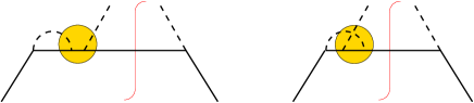
FIG. 4.: Interpretation of the one-loop corrections as final state interaction.

As a final remark, we would like to mention that the model we discussed could be applied to describe the quark distribution inside a pion in an attempt to generate T-odd distribution functions [16, 17]. However, one can readily see that, because of the different kinematical conditions, self-energy and vertex diagrams do not acquire an imaginary part, which is essential for producing a non-zero T-odd function.

In conclusion, we have shown that the Collins function can be generated using a simple pseudoscalar coupling between quarks and pions to model the fragmentation process. The Collins function turns out to be zero at the tree level due to the absence of any final state interaction which is at the origin of its existence, but renders itself at the one-loop level. The calculation performed here suggests that the Collins function, being non-zero already in a simple model, is very unlikely to vanish in reality. It is therefore a worthwhile task to pursue the measurement of $H_{1}^{\perp}$ in DIS and $e^{+}e^{-}$ annihilation. Moreover, our result supports the idea of using one-particle inclusive DIS as a promising process to investigate the transversity distribution of the nucleon.

We would like to thank E. Leader and D. Boer for useful discussions. This work is part of the research program of the Dutch Foundation for Fundamental Research on Matter (FOM) and it is partially funded by the European Commission IHP program under contract HPRN-CT-2000-00130.

REFERENCES

- [1] J. Collins, Nucl. Phys. B396 (1993) 161 [hep-ph/9208213].
- [2] J. Levelt and P. J. Mulders, Phys. Lett. B 338 (1994) 357 [hep-ph/9408257].
- [3] R. L. Jaffe and X. Ji, Phys. Rev. Lett. 71 (1993) 2547 [hep-ph/9307329].
- [4] A. Bianconi, S. Boffi, R. Jakob and M. Radici, Phys. Rev. D 62 (2000) 034008 [hep-ph/9907475].
- [5] R. L. Jaffe, X. Jin and J. Tang, Phys. Rev. Lett. 80 (1998) 1166 [hep-ph/9709322]; R. L. Jaffe, X. Jin and J. Tang, Phys. Rev. D 57 (1998) 5920 [hep-ph/9710561].
- [6] J. C. Collins, S. F. Heppelmann and G. A. Ladinsky, Nucl. Phys. B420 (1994) 565 [hep-ph/9305309]; J. C. Collins and G. A. Ladinsky, [hep-ph/9411444]; A. Bianconi, S. Boffi, R. Jakob and M. Radici, Phys. Rev. D 62 (2000) 034009 [hep-ph/9907488].
- [7] A. Airapetian et al. [HERMES Collaboration], Phys. Rev. Lett. 84 (2000) 4047 [hep-ex/9910062].
- [8] K. A. Oganessyan, H. R. Avakian, N. Bianchi and A. M. Kotzinian, hep-ph/9808368.
- [9] A. Bravar et al. [Fermilab E704 Collaboration], Phys. Rev. Lett. 77 (1996) 2626.
- [10] M. Anselmino, M. Boglione and F. Murgia, Phys. Rev. D 60 (1999) 054027 [hep-ph/9901442]; M. Boglione and P. J. Mulders, Phys. Rev. D 60 (1999) 054007 [hep-ph/9903354]; M. Boglione and E. Leader, Phys. Rev. D 61 (2000) 114001 [hep-ph/9911207]; N. I. Kochelev, JETP Lett. 72 (2000) 481 [hep-ph/9905497].
- [11] HERMES Collaboration, HERMES 00-003.
- [12] COMPASS Collaboration, CERN/SPSLC 96-14.
- [13] K. Suzuki, RIKEN Rev. 28 (2000) 105 [hep-ph/0002218].
- [14] P. J. Mulders and R. D. Tangerman, Nucl. Phys. B461 (1996) 197 [hep-ph/9510301] and Nucl. Phys. B484 (1997) 538 (E).
- [15] A. Manohar and H. Georgi, Nucl. Phys. B 234 (1984) 189.
- [16] D. Sivers, Phys. Rev. D 41 (1990) 83.
- [17] D. Boer and P. J. Mulders, Phys. Rev. D 57 (1998) 5780 [hep-ph/9711485].