Strangeness in the nucleon: neutrino–nucleon and polarized electron–nucleon scattering

Abstract

After the EMC and subsequent experiments at CERN, SLAC and DESY on the deep inelastic scattering of polarized leptons on polarized nucleons, it is now established that the $Q^{2}=0$ value of the axial strange form factor of the nucleon, a quantity which is connected with the spin of the proton and is quite relevant from the theoretical point of view, is relatively large.

In this review we consider different methods and observables that allow to obtain information on the strange axial and vector form factors of the nucleon at different values of $Q^{2}$. These methods are based on the investigation of the Neutral Current induced effects such as the P-odd asymmetry in the scattering of polarized electrons on protons and nuclei, the elastic neutrino (antineutrino) scattering on protons and the quasi–elastic neutrino (antineutrino) scattering on nuclei. We discuss in details the phenomenology of these processes and the existing experimental data.

Keywords Strangeness; strange form factors; neutrino scattering; polarized electron scattering.

1 Introduction

In this review we will discuss the strange form factors of the nucleon. As it is well known, the net strangeness of the nucleon is equal to zero. However, according to quantum field theory, in the cloud of a physical nucleon there must be pairs of strange particles. From the point of view of QCD the nucleon consists of valence $u$ and $d$ quarks and of a sea of quark–antiquark pairs $\bar{u}u$, $\bar{d}d$, $\bar{s}s$,…. produced by virtual gluons.

In the region of large $Q^{2}$ information about the $\bar{s}s$ sea can be obtained from the experiments on the production of charmed particles in charged current interactions of neutrinos and antineutrinos with nucleons in the deep inelastic region. The charmed particles can be produced in $d-c$ and $s-c$ transitions. The probability of $d-c$ transitions is proportional to $\sin^{2}\theta_{C}$, while the probability of $s-c$ transition is proportional to $\cos^{2}\theta_{C}$ ($\theta_{C}$ being the Cabibbo angle). Due to the smallness of $\theta_{C}$ ($\sin^{2}\theta_{C}\simeq 4\cdot 10^{-2}$) the $d-c$ transition is a Cabibbo–suppressed one. This enhances the possibility of studying the strange sea in the nucleon by observing two–muon neutrino events (one muon is produced by neutrinos and another muon is produced in the decay of charmed particles) [1, 2, 3, 4, 5]. In the latest NuTeV experiment at Fermilab [4] the following value was found for the ratio of the total momentum fraction carried by the strange (and anti-strange) sea quarks in the nucleon to the total momentum fraction carried by $\bar{u}$ and $\bar{d}$:

$$\kappa=\frac{S+\overline{S}}{\overline{U}+\overline{D}}=0.42\pm 0.07\pm 0.06\,.$$ (1.1)

Here $\overline{Q}=\int_{0}^{1}dx\,x\overline{q}(x)$, $\overline{q}$ being the number density of antiquarks $\overline{q}$ which carry the fraction $x$ of the proton momentum $p$ (in the infinite momentum frame). A recent analysis of deep inelastic scattering data found a larger value of $\kappa$ [6].

The investigation of the matrix elements $\langle p^{\prime}|\overline{s}\mathcal{O}s|p\rangle$ ($|p\rangle$ being the state of a nucleon with momentum $p$ and $\mathcal{O}$ some spin operator) in the confinement region $Q^{2}\lesssim 1$ GeV² is a very important subject [7, 8, 9]. Some information on this matrix element can be obtained from the pion–nucleon scattering data and from the masses of strange baryons (see Ref. [10]).

Let us consider the scalar form factor

$${\hat{m}}\langle p^{\prime}|(\overline{u}u+\overline{d}d)|p\rangle=\overline{u}(p^{\prime})u(p)\sigma_{\pi N}(t)$$ (1.2)

where

$${\hat{m}}=\frac{1}{2}(m_{u}+m_{d}),\quad t=(p^{\prime}-p)^{2}\,.$$

Chiral perturbation theory allows one to connect the value of the scalar form factor in the Cheng–Dashen point $s=u=M^{2}$, $t=2m_{\pi}^{2}$ with the isospin–even amplitude of pion–nucleon scattering [11, 12, 13, 14] ($s$, $u$, $t$ are the customary Mandelstam variables, $M$ is the mass of the nucleon, $m_{\pi}$ the mass of the pion). From the results of the phase–shift analysis of the low energy pion–nucleon data it is possible to obtain the value of the form factor at the point $t=0$, $\sigma_{\pi N}(0)$, which is called the $\sigma$–term.

The calculation of the $\sigma$–term requires an extrapolation from the point $t=2m_{\pi}^{2}$ to the point $t=0$. This procedure is based on dispersion relations and chiral perturbation theory. In Ref. [15] the value

$$\sigma_{\pi N}\simeq 45\pm 8\,\mathrm{MeV}$$ (1.3)

was found for the $\sigma$–term.

Let us define the quantity

$$y_{N}=\frac{\langle p|\overline{s}s|p\rangle}{\frac{1}{2}\langle p|(\overline{u}u+\overline{d}d)|p\rangle},$$ (1.4)

which characterizes the strange content of the nucleon. If one assumes that the breaking of SU(3) is due to the quark masses, the following relation, which connects the parameters $y_{N}$ and $\sigma_{\pi N}$ with the mass difference of the $\Lambda$ and $\Xi$ hyperons, can be derived [17]:

$$\frac{1}{3}\left(1-\frac{m_{s}}{{\hat{m}}}\right)\left(1-y_{N}\right)\sigma_{\pi N}\simeq M_{\Lambda}-M_{\Xi}$$ (1.5)

Taking into account higher–order corrections and assuming that the mass ratio $m_{s}/{\hat{m}}$ has the standard value $\simeq 25$, from (1.5) we have

$$(1-y_{N})\sigma_{\pi N}\simeq 31.8\,\mathrm{MeV}$$ (1.6)

and by combining (1.3) and (1.5) we obtain $y_{N}\simeq 0.3$.

Let us stress that there are many uncertainties in the determination of the value of the $\sigma_{\pi N}$–term and of the parameter $y_{N}$. They are mainly connected with the pion–nucleon experimental data and the extrapolation procedure. Larger values for the parameter $y_{N}$ up to $y_{N}=0.5$ were obtained by different authors (for a recent discussion, see Ref. [18]).

The most convincing evidence in favor of a non–zero value of the axial strange constant $g_{A}^{s}$ which characterizes the matrix element $\langle p|\overline{s}\gamma_{\alpha}\gamma_{5}s|p\rangle$, was found from the data of experiments on deep inelastic scattering of polarized leptons on polarized nucleons. The first indication in favor of $g_{A}^{s}\neq 0$ was obtained in the EMC experiment at CERN [19]. Subsequent experiments at CERN [20], SLAC [21, 22, 23, 24] and DESY [25, 26] confirmed the EMC result.

These experiments triggered a large number of theoretical papers in which the problem of the strangeness of the nucleon was investigated in detail (see the recent reviews [8, 9, 10, 27, 28]).

The cross section of the scattering of longitudinally polarized leptons on polarized nucleons is characterized by four dimensionless structure functions of the variables $x$ and $Q^{2}$: $F_{1}(x,Q^{2})$, $F_{2}(x,Q^{2})$, $g_{1}(x,Q^{2})$ and $g_{2}(x,Q^{2})$ (here $x=Q^{2}/2p\cdot q$, $Q^{2}=-q^{2}$, $p$ is the momentum of the initial nucleon, $q$ the momentum of the virtual photon). The functions $F_{1}(x,Q^{2})$ and $F_{2}(x,Q^{2})$ determine the unpolarized cross section, while the functions $g_{1}(x,Q^{2})$ and $g_{2}(x,Q^{2})$ characterize the part of the cross section which is proportional to the product of the polarizations of leptons and nucleons.

The measurement of the asymmetry in the deep inelastic scattering of longitudinally polarized leptons on longitudinally polarized nucleons allows one to determine the structure function $g_{1}(x,Q^{2})$.

In the framework of the naive parton model, based on the assumption that in the infinite momentum frame ($|\vec{p}\,|\to\infty$) partons (quarks) can be considered as a free particles, all structure functions depend only on the scaling variable $x$. Let us consider, in the infinite momentum frame, a nucleon with helicity equal to one. For the function $g_{1}(x)$ we have

$$g_{1}(x)=\frac{1}{2}\sum_{q}e_{q}^{2}\left[q^{(+1)}(x)+\overline{q}^{(+1)}(x)-q^{(-1)}(x)-\overline{q}^{(-1)}(x)\right]$$ (1.7)

where $e_{q}$ is the charge of the quark (in the unit of the proton charge), $q^{(\pm 1)}(x)$ ($\overline{q}^{(\pm 1)}(x)$) is the number–density of the quarks $q$ (antiquarks $\bar{q}$) with momentum $xp$ and helicity equal (respectively, opposite) to the helicity of the nucleon. Thus, the structure function $g_{1}$ is determined by the differences of the number of quarks and antiquarks with positive and negative helicities. Notice that in the naive parton model the structure functions $F_{1}(x)$ and $F_{2}(x)$ are given by

$$F_{2}(x)=x\sum_{q}e_{q}^{2}q(x)=2xF_{1}(x)\,,$$ (1.8)

where

$$q(x) = q^{(+1)}(x)+q^{(-1)}(x),$$

$$\overline{q}(x) = \overline{q}^{(+1)}(x)+\overline{q}^{(-1)}(x)$$

are the total numbers of quarks and antiquarks with momentum $xp$.

From the theoretical point of view, the important quantity is the first moment of the structure function $g_{1}$:

$$\Gamma_{1}(Q^{2})=\int_{0}^{1}g_{1}(x,Q^{2})dx\,.$$ (1.9)

In the region $Q^{2}\lesssim 10$ GeV² the main contribution to $\Gamma_{1}$ comes from the light $u,d,s$ quarks.

In the naive parton model, for the first moment of the proton we have

$$\Gamma_{1}^{p}=\frac{1}{2}\left(\frac{4}{9}\Delta u+\frac{1}{9}\Delta d+\frac{1}{9}\Delta s\right)$$ (1.10)

where

$$\Delta q=\int_{0}^{1}\sum_{r=\pm 1}r\left[q^{(r)}(x)+\overline{q}^{(r)}(x)\right]dx$$ (1.11)

is the difference of the total numbers of quarks and antiquarks in the nucleon with helicity equal and opposite to the helicity of the nucleon. Thus $\Delta q$ is the contribution of the $q$-quarks and $\bar{q}$-antiquarks to the spin of the proton.

The first moment $\Gamma_{1}^{p}$ can be determined from the measurement of the deep inelastic scattering of polarized leptons on longitudinally polarized protons. In the EMC experiment at $Q^{2}=10.7$ GeV² the value

$$\Gamma_{1}^{p}(10.7)=0.126\pm 0.010\pm 0.015$$ (1.12)

was found, while in the latest CERN SMC [20], SLAC 155 [24] and DESY HERMES [25, 26] experiments the following values of $\Gamma_{1}^{p}$ were determined:

$$\Gamma_{1}^{p}(10) = 0.120\pm 0.005\pm 0.006\pm 0.014$$

$$\Gamma_{1}^{p}(5) = 0.118\pm 0.004\pm 0.007$$ (1.13)

$$\Gamma_{1}^{p}(3) = 0.122\pm 0.003\pm 0.010$$

Let us stress that the experimental data can be obtained in a limited interval of the variable $x$ which does not include the region of very small and very large values of $x$. In order to determine the value of $\Gamma_{1}^{p}$ it is necessary to make extrapolations of the data to the points $x=0$ and $x=1$. The small $x$–behavior of the structure function $g_{1}$ is the most contradictory issue (see Ref. [8]). Usually a Regge–behavior of the function $g_{1}$ is assumed at small $x$. Recent extrapolations are based on NLO (next to leading order) QCD fits. Notice that in some non–perturbative approaches a singular behavior of the function $g_{1}(x)$ at small $x$ was obtained [8].

Let us now discuss the possibilities of determining the axial strange constant $g_{A}^{s}$ from these data.

In the framework of the naive parton model the quantities $\Delta q$, which enter into the sum rule (1.10), are determined by the one–nucleon matrix element of the axial quark current $\overline{q}\gamma_{\alpha}\gamma_{5}q$ (see Section 3):

$${{}_{p}\langle}p|\overline{q}\gamma_{\alpha}\gamma_{5}q|p\rangle_{p}=2Ms_{\alpha}\Delta q$$ (1.14)

Here $s_{\alpha}$ is the polarization vector of the nucleon and $|p\rangle_{p}$ ($|p\rangle_{n}$) is the state vector of a proton (neutron) with momentum $p$. The relation (1.14) allows one to obtain two constraints on the quantities $\Delta u$, $\Delta d$ and $\Delta s$. The first one comes from the isotopic SU(2) invariance of strong interactions, which implies:

$${{}_{p}\langle}p|\overline{u}\gamma_{\alpha}\gamma_{5}d|p\rangle_{n}={{}_{p}\langle}p|\left(\overline{u}\gamma_{\alpha}\gamma_{5}u-\overline{d}\gamma_{\alpha}\gamma_{5}d\right)|p\rangle_{p}\,.$$ (1.15)

From (1.15) and (1.14) it follows that

$$\Delta u-\Delta d=g_{A}$$ (1.16)

where $g_{A}$ is the weak axial constant. From the data on the $\beta$–decay of the neutron it follows that [29]:

$$g_{A}=1.2670\pm 0.0035\,.$$ (1.17)

The second constraint follows from SU(3) symmetry. Assuming exact SU(3) symmetry we have

$$\Delta u+\Delta d-2\Delta s=3F-D\equiv g_{A}^{8}$$ (1.18)

where $F$ and $D$ are the constants which determine the matrix elements of the axial weak current for the states of different hyperons belonging to the SU(3) octet. From the fit of the experimental data it was found that [29]:

$$F=0.463\pm 0.008;\qquad D=0.804\pm 0.008$$ (1.19)

hence

$$g_{A}^{8}=0.585\pm 0.025$$ (1.20)

Now from Eqs. (1.10), (1.17) and (1.19) we can express the first moment as follows:

$$\Gamma_{1}^{p}=0.187\pm 0.004+\frac{1}{3}\Delta s\,.$$ (1.21)

If we compare (1.21) with the values of $\Gamma_{1}^{p}$ which were obtained in experiments [see (1.12) and (1.13)], we come to the conclusion that the quantity $\Delta s$, which determines the matrix element of the strange axial current, is different from zero and negative. Using, for example, the EMC result (1.12), from (1.21) we find

$$\Delta s=-0.18\pm 0.05\,.$$

This conclusion is based on the naive parton model and was obtained about 10 years ago (see Ref. [7]). After the EMC result was obtained, a lot of experimental and theoretical works were published. The LO (leading order) and NLO QCD corrections to the sum rule (1.10) and to the relation (1.15) were calculated and many different effects were taken into account (see the reviews [8, 9, 10, 27, 28, 30, 31, 32, 33]).

Let us introduce the constants $A_{i}$

$${{}_{p}\langle}p|\overline{\psi}\gamma_{\alpha}\gamma_{5}\lambda_{i}\psi|p\rangle_{p}=2Ms_{\alpha}A_{i}\quad(i=3,8)$$ (1.22)

and

$${{}_{p}\langle}p|\overline{\psi}\gamma_{\alpha}\gamma_{5}\psi|p\rangle_{p}=2Ms_{\alpha}A_{0}$$ (1.23)

where $\psi=\left(\begin{array}[]{c}u\\ d\\ s\end{array}\right)$ is the flavor SU(3) triplet, $\lambda_{i}$ are the Gell–Mann matrices, $\overline{\psi}\gamma_{\alpha}\gamma_{5}\lambda_{i}\psi$ is the SU(3) octet of axial currents and $\overline{\psi}\gamma_{\alpha}\gamma_{5}\psi$ the axial singlet current.

In the naive parton model the following relations hold:

$$A_{3} = \Delta u-\Delta d=g_{A}^{3}\equiv g_{A}$$

$$A_{8} = \Delta u+\Delta d-2\Delta s\equiv g_{A}^{8}$$ (1.24)

$$A_{0} = \Delta u+\Delta d+\Delta s=g_{A}^{0}\equiv\Delta\Sigma$$

the quantity $\Delta\Sigma$ being the total contribution of quarks and antiquarks to the spin of the proton. The sum rule (1.10) can be now rewritten in the form

$$\Gamma_{1}^{p}=\frac{1}{12}A_{3}+\frac{1}{36}A_{8}+\frac{1}{9}A_{0}\,.$$ (1.25)

The NLO QCD corrections modify the above expression as follows (see [8] and references therein):

$$\Gamma_{1}^{p}(Q^{2})=\left(1-\frac{\alpha_{s}(Q^{2})}{\pi}\right)\left[\frac{1}{12}A_{3}+\frac{1}{36}A_{8}+\frac{1}{9}A_{0}(Q^{2})\right]$$ (1.26)

where $\alpha_{s}(Q^{2})$ is the strong coupling constant and the quantities $A_{i}$ ($i=3,8,0$) are given by the relation (1.22). The quantities $A_{3}$ and $A_{8}$ are determined by the one–nucleon matrix elements of the corresponding conserved currents (we have assumed SU(3) flavor symmetry). These quantities do not depend on $Q^{2}$ and turn out to be

$$A_{3}=g_{A}\,~{}~{}~{}A_{8}=g_{A}^{8}\,,$$ (1.27)

where the numerical values of the constants $g_{A}$ and and $g_{A}^{8}$ are given by Eqs. (1.17) and (1.20), respectively. The quantity $A_{0}$, instead, is determined by the matrix element of the non–conserved singlet current $\bar{\psi}\gamma^{\alpha}\gamma_{5}\psi$. If higher order QCD corrections are taken into account, then this quantity depends on the renormalization scheme and on the renormalization scale, which is usually taken to be equal to $Q^{2}$.

Two renormalization schemes are commonly employed: the $\overline{\rm{MS}}$ scheme [34] and the AB (Adler–Bardeen) scheme [35]. In the $\overline{\rm{MS}}$ scheme $A_{0}(Q^{2})$ is determined by the renormalization scale–dependent contribution of quarks to the spin of nucleon,

$$A_{0}(Q^{2})=\Delta\Sigma(Q^{2})=\sum_{q=u,d,s}\Delta q(Q^{2})\,.$$ (1.28)

In the AB scheme $A_{0}(Q^{2})$ is determined by the contribution of quarks and gluons to the spin of the proton

$$A_{0}(Q^{2})=\Delta\Sigma^{AB}-3\frac{\alpha_{s}(Q^{2})}{2\pi}\Delta G(Q^{2})$$ (1.29)

where $\Delta\Sigma^{AB}$ does not depend on $Q^{2}$ and all renormalization scale dependence is absorbed by the gluon contribution $\Delta G(Q^{2})$. The latter, due to triangle anomaly [36, 37], behaves as $1/\alpha_{s}$ and can give a sizable contribution to $A_{0}(Q^{2})$.

In the $\overline{\rm{MS}}$ scheme, from Eqs. (1.14), (1.24) and (1.26), for the matrix element of the axial strange current in NLO approximation we have

$$\frac{1}{2M}\langle p|\overline{s}\gamma_{\alpha}\gamma_{5}s|p\rangle s^{\alpha}=-3\left(1-\frac{\alpha_{s}(Q^{2})}{\pi}\right)^{-1}\Gamma_{1}^{p}(Q^{2})+\frac{1}{4}g_{A}+\frac{5}{12}g_{A}^{8}\,.$$ (1.30)

Let us stress that the matrix element $\langle p|\overline{s}\gamma_{\alpha}\gamma_{5}s|p\rangle$ depends on the renormalization scale. Using the E155 data [24] at $Q^{2}=5~{}\rm{GeV}^{2}$ and the values (1.17), (1.20) of the axial constants $g_{A}$ and $g_{A}^{8}$, from (1.30) we find

$$\frac{1}{2M}\langle p|\overline{s}\gamma_{\alpha}\gamma_{5}s|p\rangle s^{\alpha}=0.12\pm 0.03$$ (1.31)

Thus, if we take into account higher order QCD corrections, from the data on deep inelastic scattering of polarized leptons on polarized protons we can conclude that the one–nucleon matrix element of the axial strange current is relatively large. This conclusion does not depend on the renormalization scheme (matrix elements are measurable quantities). Similar considerations can be drawn from the operator product expansion (OPE) approach [38].

In this review we will consider possibilities of obtaining information on the strange vector and axial form factors of the nucleon from the investigation of neutral current effects. We will consider in detail the P–odd asymmetry in elastic and quasi–elastic scattering of polarized electrons on nucleons and nuclei (Sections 5, 6, 7, 8) and the elastic and quasi–elastic scattering of neutrinos (antineutrinos) on nucleons and nuclei (Sections 9, 10, 11, 12). We will discuss the existing experimental data and future experiments. Derivations of many basic relations will be presented.

2 The Standard Lagrangian of the interaction of leptons and quarks with vector bosons

In the Standard SU(2)$\times$U(1) electroweak Model (SM) [39, 40, 41] the Lagrangian of the interaction of the fundamental fermions (neutrinos, charged leptons and quarks) with vector bosons contains three parts: charged current (CC), electromagnetic (em) and neutral current (NC) interactions [14, 42, 43, 44, 45, 46].

2.1 The charged current Lagrangian

The Lagrangian of the CC interaction of leptons and quarks with the charged vector bosons $W^{\pm}$ reads:

$${\mathcal{L}}^{CC}_{I}=-\frac{g}{2\sqrt{2}}\,j_{\alpha}^{CC}W^{\alpha}+\mathrm{h.c.}$$ (2.1)

Here $g$ is a coupling constant which is connected with Fermi constant $G_{F}$ by the relation

$$\frac{G_{F}}{\sqrt{2}}=\frac{g^{2}}{8m_{\scriptscriptstyle W}^{2}}$$ (2.2)

($m_{\scriptscriptstyle W}$ being the mass of the W–boson) and

$$j_{\alpha}^{CC}=2\left(j_{\alpha}^{1}+ij_{\alpha}^{2}\right)\equiv 2j_{\alpha}^{1+i2}$$ (2.3)

is the charged current. In Eq. (2.3) $j_{\alpha}^{1,2}$ are components of the isovector current:

$$j_{\alpha}^{i}=\sum_{a}\overline{\psi}_{aL}\gamma_{\alpha}\frac{1}{2}\tau^{i}\psi_{aL}$$ (2.4)

where $\psi_{aL}=\frac{1}{2}(1-\gamma_{5})\psi_{a}$ are left–handed doublets of the SU(2)xU(1) gauge group of the Standard Model:

$$\begin{array}[]{lll}\psi_{eL}=\left(\begin{array}[]{c}\nu_{eL}\\ e_{L}\end{array}\right),&\psi_{\mu L}=\left(\begin{array}[]{c}\nu_{\mu L}\\ \mu_{L}\end{array}\right),&\psi_{\tau L}=\left(\begin{array}[]{c}\nu_{\tau L}\\ \tau_{L}\end{array}\right)\\ \psi_{1L}=\left(\begin{array}[]{c}u_{L}^{\prime}\\ d_{L}^{\prime}\end{array}\right),&\psi_{2L}=\left(\begin{array}[]{c}c_{L}^{\prime}\\ s_{L}^{\prime}\end{array}\right),&\psi_{3L}=\left(\begin{array}[]{c}t_{L}^{\prime}\\ b_{L}^{\prime}\end{array}\right)\end{array}$$ (2.5)

In terms of the fields of leptons and quarks with definite masses the charged current (2.4) reads:

$$j_{\alpha}^{CC}=2\sum_{\ell=e,\mu,\tau}{\overline{\nu}_{\ell}}_{L}\gamma_{\alpha}\ell_{L}+2\left[{\overline{u}}_{L}\gamma_{\alpha}d^{\mathrm{mix}}_{L}+{\overline{c}}_{L}\gamma_{\alpha}s^{\mathrm{mix}}_{L}+{\overline{t}}_{L}\gamma_{\alpha}b^{\mathrm{mix}}_{L}\right]$$ (2.6)

where now

$$d^{\mathrm{mix}}_{L}=\sum_{q=d,s,b}V_{uq}q_{L},\quad s^{\mathrm{mix}}_{L}=\sum_{q=d,s,b}V_{cq}q_{L},\quad b^{\mathrm{mix}}_{L}=\sum_{q=d,s,b}V_{tq}q_{L},\quad$$ (2.7)

and $V$ is the unitary $3\times 3$ Cabibbo–Kobayashi–Maskawa mixing matrix.

2.2 The electromagnetic interaction Lagrangian

The Lagrangian of the electromagnetic interaction has the form:

$${\mathcal{L}}^{em}_{I}=-ej_{\alpha}^{em}A^{\alpha}\,,$$ (2.8)

$e$ being the charge of the proton and

$$j_{\alpha}^{em}=\sum_{\ell=e,\mu,\tau}(-1){\overline{\ell}}\gamma_{\alpha}\ell+\sum_{q=u,d,\dots}e_{q}{\overline{q}}\gamma_{\alpha}q$$ (2.9)

the electromagnetic current (with $e_{u}=2/3$, $e_{d}=-1/3$, …)

2.3 The neutral current Lagrangian

The Lagrangian of the NC interaction of leptons and quarks with the neutral vector boson $Z^{0}$ is:

$${\mathcal{L}}^{NC}_{I}=-\frac{g}{2\cos\theta_{W}}j_{\alpha}^{NC}Z^{\alpha}\,,$$ (2.10)

where $\theta_{W}$ is the weak (Weinberg) angle, the characteristic parameter of the electroweak unification, and $j_{\alpha}^{NC}$ is the neutral current. The structure of the latter in the Standard Model is determined by the requirements of unification of the weak and electromagnetic interactions into the unified electroweak interaction. We have

$$j_{\alpha}^{NC}=2j_{\alpha}^{3}-2\sin^{2}\theta_{W}j_{\alpha}^{em}\,.$$ (2.11)

From Eqs. (2.4), (2.5) and (2.11) the neutral current can be rewritten in the following form:

$$j_{\alpha}^{NC} =\sum_{q=u,c,t}\overline{q}\gamma_{\alpha}(1-\gamma_{5})\frac{1}{2}q+\sum_{q=d,s,b}\overline{q}\gamma_{\alpha}(1-\gamma_{5})\left(-\frac{1}{2}\right)q+$$ (2.12)

$$+\sum_{\ell=e,\mu,\tau}\overline{\nu}_{\ell}\gamma_{\alpha}(1-\gamma_{5})\frac{1}{2}\nu_{\ell}+\sum_{\ell=e,\mu,\tau}\overline{\ell}\gamma_{\alpha}(1-\gamma_{5})\left(-\frac{1}{2}\right)\ell+$$

$$-2\sin^{2}\theta_{W}j_{\alpha}^{em}\,.$$

In this review we will focus on processes at relatively small energies (less than a few GeV). Therefore it can be convenient to separate, in (2.12), the contribution of the lightest $u$ and $d$ quarks. One obtains:

$$j_{\alpha}^{NC;q}=v_{\alpha}^{3}-a_{\alpha}^{3}-\frac{1}{2}\left(v_{\alpha}^{s}-a_{\alpha}^{s}\right)-2\sin^{2}\theta_{W}j_{\alpha}^{em}\,.$$ (2.13)

Here we define:

$$v_{\alpha}^{3} =\overline{u}\gamma_{\alpha}\frac{1}{2}u-\overline{d}\gamma_{\alpha}\frac{1}{2}d\equiv{\overline{N}}\gamma_{\alpha}\frac{1}{2}\tau_{3}N,$$

$$a_{\alpha}^{3} =\overline{u}\gamma_{\alpha}\gamma_{5}\frac{1}{2}u-\overline{d}\gamma_{\alpha}\gamma_{5}\frac{1}{2}d\equiv{\overline{N}}\gamma_{\alpha}\gamma_{5}\frac{1}{2}\tau_{3}N,$$

where $N=\scriptscriptstyle{\left(\begin{array}[]{c}u\\ d\end{array}\right)}$. Indeed the mass difference between $d$ and $u$ quarks ($m_{d}-m_{u}\simeq 3$ MeV [29] is much smaller than the QCD constant $\Lambda^{\mathrm{QCD}}\simeq 200\div 300$ MeV and can be neglected: in this case $N$ is a doublet of the isotopic SU(2) group and the currents $v^{3}_{\alpha}$ and $a^{3}_{\alpha}$ are the third components of the isovectors

$$v_{\alpha}^{i}=\overline{N}\gamma_{\alpha}\frac{1}{2}\tau^{i}N,\quad a^{i}_{\alpha}=\overline{N}\gamma_{\alpha}\gamma_{5}\frac{1}{2}\tau^{i}N\,.$$ (2.14)

Instead, the currents $v^{s}_{\alpha}$ and $a^{s}_{\alpha}$ are isoscalars: they represent the contributions to $j_{\alpha}^{NC;q}$ of the $s$, $c$ and heavier quarks. Taking into account only $s$–quarks we have

$$v_{\alpha}^{s}=\overline{s}\gamma_{\alpha}s,\quad a_{\alpha}^{s}=\overline{s}\gamma_{\alpha}\gamma_{5}s$$ (2.15)

The quark electromagnetic current is given by [see Eq. (2.9)]

$$j_{\alpha}^{em;q}=\sum_{q=u,d,\dots}e_{q}\overline{q}\gamma_{\alpha}q$$ (2.16)

Also in this case it is convenient to separate, in the above current, the contributions of the lightest $u$, $d$ quarks. Taking into account that $e_{q}=I_{3}^{q}+\scriptstyle{\frac{1}{6}}$ ($q=u,d$) we have:

$$j_{\alpha}^{em;q}=v_{\alpha}^{3}+v_{\alpha}^{0}$$ (2.17)

where $v_{\alpha}^{0}$ is the isoscalar current which, in the $u$, $d$, $s$ approximation, reads:

$$v_{\alpha}^{0}=\frac{1}{6}\overline{N}\gamma_{\alpha}N+\left(-\frac{1}{3}\right)\overline{s}\gamma_{\alpha}s\,.$$ (2.18)

3 One-nucleon matrix elements of the neutral current

We will considerer here in detail the one–nucleon matrix elements of the neutral current as well as the ones of the electromagnetic current. Let us consider, for example, the process of the elastic scattering of muon–neutrino on the nucleon:

$$\nu_{\mu}+p\longrightarrow\nu_{\mu}+p$$ (3.1)

The amplitude of this process is given by the expression

$$\langle f|S|i\rangle=$$ (3.2)

$$\quad=-i\frac{G_{F}}{\sqrt{2}}\overline{u}(k^{\prime})\gamma^{\alpha}(1-\gamma_{5})u(k)\,_{\mathrm{out}}\langle p^{\prime}|J_{\alpha}^{NC}(0)|p\rangle_{\mathrm{in}}(2\pi)^{4}\delta^{(4)}(p^{\prime}-p-q)$$

where $k$ and $p$ ($k^{\prime}$ and $p^{\prime}$) are the four–momenta of the initial (final) neutrino and nucleon, respectively, $q=k-k^{\prime}$ and

$$_{\mathrm{out}}\langle p^{\prime}|J_{\alpha}^{NC}(0)|p\rangle_{\mathrm{in}}=\langle p^{\prime}|T\left\{j_{\alpha}^{NC}(0)e^{-i\int\,{\mathcal{H}}_{I}^{had}(x)d^{4}x}\right\}|p\rangle$$ (3.3)

is the hadronic matrix element.

In Eq. (3.3) ${\mathcal{H}}_{I}^{had}(x)$ is the Hamiltonian density of the strong interactions, $J_{\alpha}^{NC}(0)$, $|p\rangle_{\mathrm{in}}$ and $|p\rangle_{\mathrm{out}}$ are the neutral current operator, the initial and final nucleon states in the Heisenberg representation.

From (2.13) we get the following expression for the matrix element of the neutral current:

$$\langle p^{\prime}|J_{\alpha}^{NC}(0)|p\rangle =\langle p^{\prime}|\left(V^{3}_{\alpha}-A^{3}_{\alpha}\right)|p\rangle-\frac{1}{2}\langle p^{\prime}|\left(V^{s}_{\alpha}-A^{s}_{\alpha}\right)|p\rangle+$$ (3.4)

$$\qquad-2\sin^{2}\theta_{W}\langle p^{\prime}|J_{\alpha}^{em}|p\rangle$$

where $V^{3(s)}_{\alpha}$, $A^{3(s)}_{\alpha}$ are the currents in Heisenberg representation. From the isotopic SU(2) invariance of strong interactions it follows that $V^{3}_{\alpha}$, $A^{3}_{\alpha}$ are the third components of the isovector currents $V^{i}_{\alpha}$ and $A^{i}_{\alpha}$ ($i=1,2,3$) while $V^{s}_{\alpha}$, $A^{s}_{\alpha}$ are isoscalar currents.

The isotopic invariance of strong interactions allows one to determine the one–nucleon matrix elements of the current $V_{\alpha}^{3}$ from the one–nucleon matrix elements of the electromagnetic current $J^{em}_{\alpha}$. In fact, from (2.17) it follows

$${{}_{p(n)}\langle}p^{\prime}|J_{\alpha}^{em}|p\rangle_{p(n)}={{}_{p(n)}\langle}p^{\prime}|V_{\alpha}^{3}|p\rangle_{p(n)}+{{}_{p(n)}\langle}p^{\prime}|V_{\alpha}^{0}|p\rangle_{p(n)}$$ (3.5)

where $|p\rangle_{p}$ ($|p\rangle_{n}$) is the state of a proton (neutron) with momentum $p$. Furthermore we have

$$\mathcal{U}V_{\alpha}^{3}\mathcal{U}^{-1}=-V^{3}_{\alpha},\quad\mathcal{U}V_{\alpha}^{0}\mathcal{U}^{-1}=V^{0}_{\alpha},$$ (3.6)

where the charge symmetry operator $\mathcal{U}=\exp\{i\pi I_{2}\}$ (rotation of $\pi$ around the second axis in the isotopic space) transforms proton states into neutron states and viceversa, according to:

$$\mathcal{U}|p\rangle_{p}=-|p\rangle_{n},\quad\mathcal{U}|p\rangle_{n}=|p\rangle_{p}\,.$$

The following relations then hold:

$$\begin{array}[]{ll}{{}_{p}\langle}p^{\prime}|V_{\alpha}^{3}|p\rangle_{p}=-&{{}_{n}\langle}p^{\prime}|V_{\alpha}^{3}|p\rangle_{n}\,,\\ {{}_{p}\langle}p^{\prime}|V_{\alpha}^{0}|p\rangle_{p}=+&{{}_{n}\langle}p^{\prime}|V_{\alpha}^{0}|p\rangle_{n}\end{array}$$ (3.7)

From (3.5) and (3.7) we have then:

$${{}_{p}\langle}p^{\prime}|V_{\alpha}^{3}|p\rangle_{p}=\frac{1}{2}\left[{{}_{p}\langle}p^{\prime}|J_{\alpha}^{em}|p\rangle_{p}-{{}_{n}\langle}p^{\prime}|J_{\alpha}^{em}|p\rangle_{n}\right]\,.$$ (3.8)

Moreover

$${{}_{p}\langle}p^{\prime}|V_{\alpha}^{0}|p\rangle_{p}=\frac{1}{2}\left[{{}_{p}\langle}p^{\prime}|J_{\alpha}^{em}|p\rangle_{p}+{{}_{n}\langle}p^{\prime}|J_{\alpha}^{em}|p\rangle_{n}\right]\,.$$ (3.9)

Let us discuss now the one–nucleon matrix elements of the electromagnetic current. The conservation law of the electromagnetic current, $\partial^{\alpha}J_{\alpha}^{em}=0$, entails

$$(p^{\prime}-p)\langle p^{\prime}|J_{\alpha}^{em}|p\rangle=0\,.$$ (3.10)

From this relation it follows that the one–nucleon matrix elements of the electromagnetic current are characterized by two form factors and have the general form

$$\langle p^{\prime}|J_{\alpha}^{em}|p\rangle=\overline{u}(p^{\prime})\left[\gamma_{\alpha}F_{1}(Q^{2})+\frac{i}{2M}\sigma_{\alpha\beta}q^{\beta}F_{2}(Q^{2})\right]u(p)$$ (3.11)

Here $q=p^{\prime}-p$ is the four–momentum transfer, $Q^{2}=-q^{2}$, $\sigma_{\alpha\beta}={\scriptstyle\frac{i}{2}}(\gamma_{\alpha}\gamma_{\beta}-\gamma_{\beta}\gamma_{\alpha})$, $F_{1}(Q^{2})$ and $F_{2}(Q^{2})$ are the Dirac and Pauli form factors . At $Q^{2}=0$ we have

$$F_{1}(0)=e_{N},\quad F_{2}(0)=\kappa_{N}$$ (3.12)

where $e_{N}$ is the nucleon charge (in units of the proton charge) and $\kappa_{N}$ is the anomalous magnetic moment of the nucleon (in units of the nucleon Bohr magneton). Notice that from the invariance of strong interactions under time reversal it follows that the form factors are real functions of $Q^{2}$.

With the help of the Dirac equation the matrix element (3.11) can be rewritten in the form:

$$\langle p^{\prime}|J_{\alpha}^{em}|p\rangle=\overline{u}(p^{\prime})\left[\gamma_{\alpha}G_{M}(Q^{2})-n_{\alpha}\frac{1}{2M}\frac{G_{M}(Q^{2})-G_{E}(Q^{2})}{1+\tau}\right]u(p)$$ (3.13)

Here $n=p+p^{\prime}$, $\tau=Q^{2}/4M^{2}$ and

$$\begin{array}[]{ll}G_{M}(Q^{2})=&F_{1}(Q^{2})+F_{2}(Q^{2})\\ G_{E}(Q^{2})=&F_{1}(Q^{2})-\tau F_{2}(Q^{2})\end{array}$$ (3.14)

are, correspondingly, the magnetic and electric (charge) Sachs form factors . In the $Q^{2}=0$ limit they yield

$$G_{M}(0) =e_{N}+\kappa_{N}=\mu_{N}$$

$$G_{E}(0) =e_{N}$$

$\mu_{N}$ being the total magnetic moment of the nucleon (in units of the nucleon Bohr magneton).

Let us notice that the magnetic and electric form factors $G_{M}$ and $G_{E}$ characterize the matrix elements of the operators ${\vec{J}}^{em}$ and $J_{0}^{em}$, respectively, in the Breit system (the system in which ${\vec{n}}={\vec{p}}+{\vec{p^{\prime}}}=0$). In fact, from (3.13) it follows that

$$\langle p^{\prime}|{\vec{J}}^{em}|p\rangle=\overline{u}(p^{\prime}){\vec{\gamma}}u(p)G_{M}(Q^{2})\,.$$ (3.15)

Furthermore, in the Breit system $n_{0}=2p_{0}$ and we have

$$\langle p^{\prime}|J_{0}^{em}|p\rangle=\overline{u}(p^{\prime})\left[\gamma_{0}G_{M}(Q^{2})-\frac{p_{0}}{M}\frac{G_{M}(Q^{2})-G_{E}(Q^{2})}{1+\tau}\right]u(p)\,,$$ (3.16)

while, from the Dirac equation, it follows:

$$\overline{u}(p^{\prime})({\hbox to0.0pt{/\hss}{p}}^{\prime}+\hbox to0.0pt{/\hss}{p})u(p)=2p_{0}\overline{u}(p^{\prime})\gamma_{0}u(p)=2M\overline{u}(p^{\prime})u(p)\,.$$ (3.17)

The quantity $p_{0}^{2}/M^{2}$ in the Breit system can be expressed through:

$$\frac{p_{0}^{2}}{M^{2}}=1+\frac{Q^{2}}{4M^{2}}\equiv 1+\tau\,,$$

and combining (3.16) and (3.17) we have

$$\langle p^{\prime}|J_{0}^{em}|p\rangle=\overline{u}(p^{\prime})\gamma_{0}u(p)G_{E}(Q^{2})\,.$$ (3.18)

Let’s consider now the one–nucleon matrix elements of the vector current. From the relation (3.8) it follows:

$${{}_{p}\langle}p^{\prime}|V_{\alpha}^{3}|p\rangle_{p}=-{{}_{n}\langle}p^{\prime}|V_{\alpha}^{3}|p\rangle_{n}=$$ (3.19)

$$\qquad\quad=\overline{u}(p^{\prime})\left[\gamma_{\alpha}F_{1}^{V}(Q^{2})+\frac{i}{2M}\sigma_{\alpha\beta}q^{\beta}F_{2}^{V}(Q^{2})\right]u(p)$$

where

$$F_{1}^{V}(Q^{2}) = \frac{1}{2}\left({F_{1}}_{\!,p}(Q^{2})-{F_{1}}_{\!,n}(Q^{2})\right)\,,$$

$$F_{2}^{V}(Q^{2}) = \frac{1}{2}\left({F_{2}}_{\!,p}(Q^{2})-{F_{2}}_{\!,n}(Q^{2})\right)\,,$$

are the isovector Dirac and Pauli form factors . Alternatively we can use the isovector magnetic and electric (charge) form factors :

$$G_{M}^{V}(Q^{2}) = \frac{1}{2}\left({G_{M}}_{\!,p}(Q^{2})-{G_{M}}_{\!,n}(Q^{2})\right)\,,$$

$$G_{E}^{V}(Q^{2}) = \frac{1}{2}\left({G_{E}}_{\!,p}(Q^{2})-{G_{E}}_{\!,n}(Q^{2})\right)\,.$$

Let us consider now the one–nucleon matrix elements of the operator $A_{\alpha}^{3}$. Information about these matrix elements can be obtained from the data on the investigation of the quasi–elastic processes

$$\nu_{\mu}+n \longrightarrow\mu^{-}+p$$ (3.20)

$$\overline{\nu}_{\mu}+p \longrightarrow\mu^{+}+n$$ (3.21)

In the region $Q^{2}\ll m_{W}^{2}$ we are interested in, the matrix elements of the processes (3.20) and (3.21) have the following form

$$\langle f|S|i\rangle =-i\frac{G_{F}}{\sqrt{2}}\overline{u}(k^{\prime})\gamma^{\alpha}(1-\gamma_{5})u(k){{}_{p}\langle}p^{\prime}|J_{\alpha}^{CC}|p\rangle_{n}\,(2\pi)^{4}\delta^{(4)}(p^{\prime}-p-q)$$

$$\langle f|S|i\rangle =-i\frac{G_{F}}{\sqrt{2}}\overline{u}(k^{\prime})\gamma^{\alpha}(1+\gamma_{5})u(k){{}_{n}\langle}p^{\prime}|{J_{\alpha}^{CC}}^{\dagger}|p\rangle_{p}\,(2\pi)^{4}\delta^{(4)}(p^{\prime}-p-q)$$

Here $k$ is the momentum of the initial $\nu_{\mu}$ ($\bar{\nu}_{\mu}$), $k^{\prime}$ the momentum of the final $\mu^{-}$ ($\mu^{+}$); $p$ and $p^{\prime}$ are the momenta of the initial $n$ ($p$) and of the final $p$ ($n$), respectively.

The quark current which gives contribution to the matrix element of the process (3.20) has the form

$$j_{\alpha}^{CC}=\overline{u}\gamma_{\alpha}(1-\gamma_{5})d\,V_{ud}$$ (3.22)

where $V_{ud}$ is an element of the CKM mixing matrix. From the existing data $|V_{ud}|^{2}=0.9735\pm 0.0008$ [29] and hereafter we will not take into account small corrections due to $|V_{ud}|\neq 1$. The current (3.22) can be expressed in terms of the above introduced $u$, $d$ quark iso–doublet $N$ as follows:

$$j_{\alpha}^{CC}=\overline{N}\gamma_{\alpha}(1-\gamma_{5})\frac{1}{2}(\tau_{1}+i\tau 2)N\equiv v_{\alpha}^{1+i2}-a_{\alpha}^{1+i2}\,,$$ (3.23)

where $v_{\alpha}^{1+i2}$ and $a_{\alpha}^{1+i2}$ are the “plus–components” of the isovectors (2.14).

For the Heisenberg currents we have

$$J_{\alpha}^{CC}=V_{\alpha}^{1+i2}-A_{\alpha}^{1+i2}\,,$$ (3.24)

where $V_{\alpha}^{1+i2}$ and $A_{\alpha}^{1+i2}$ are the “plus-components” of the isovectors $V_{\alpha}^{i}$ and $A_{\alpha}^{i}$.

Let us consider now the one–nucleon matrix elements of the axial current. The charge symmetry operator $\mathcal{U}$ introduced in (3.6) transforms the isovector $A_{\alpha}^{i}$ as follows:

$$\begin{array}[]{lr}\mathcal{U}A_{\alpha}^{1,3}\mathcal{U}^{-1}&=-A_{\alpha}^{1,3}\\ \mathcal{U}A_{\alpha}^{2}\mathcal{U}^{-1}&=A_{\alpha}^{2}\end{array}$$ (3.25)

From these relations we have:

$${{}_{p}\langle}p^{\prime}|A_{\alpha}^{1+i2}|p\rangle_{n}={{}_{n}\langle}p^{\prime}|A_{\alpha}^{1-i2}|p\rangle_{p}\,.$$ (3.26)

Eq. (3.26) implies:

$${{}_{p}\langle}p^{\prime}|A_{\alpha}^{1+i2}|p\rangle_{n}={{}_{p}\langle}p|A_{\alpha}^{1+i2}|p^{\prime}\rangle_{n}^{*}$$ (3.27)

The one–nucleon matrix element of the CC axial current has the following general structure

$${{}_{p}\langle}p^{\prime}|A_{\alpha}^{1+i2}|p\rangle_{n}=$$ (3.28)

$$\qquad=\overline{u}(p^{\prime})\left[\gamma_{\alpha}\gamma_{5}G_{A}(Q^{2})+\frac{1}{2M}q_{\alpha}\gamma_{5}G_{P}^{CC}(Q^{2})+\frac{1}{2M}n_{\alpha}\gamma_{5}G_{T}^{CC}(Q^{2})\right]u(p)$$

Due to the invariance under time reversal the form factors $G_{A}$, $G_{P}^{CC}$ and $G_{T}^{CC}$ are real quantities. Moreover, taking into account the relation (3.27), one easily finds that

$$G_{T}^{CC}(Q^{2})=0\,.$$ (3.29)

Let us notice that for the quasi–elastic processes $\overline{u}(k^{\prime})\gamma^{\alpha}(1-\gamma_{5})u(k)q_{\alpha}=-m_{\mu}\overline{u}(k^{\prime})(1-\gamma_{5})u(k)$. Thus the contribution of the pseudoscalar form factor $G_{P}^{CC}$ to the matrix element of the processes (3.20) and (3.21) is proportional to the muon mass $m_{\mu}$ and in the region of neutrino energies $\geq 1$ GeV can be neglected.

Isotopic invariance of the strong interactions provides the relation between the one–nucleon matrix elements of the operators $A_{\alpha}^{3}$ and $A_{\alpha}^{1+i2}$. In fact for the isovector $A_{\alpha}^{i}$ we have

$$\left[I_{k},A_{\alpha}^{j}\right]=i\epsilon_{kj\ell}A_{\alpha}^{\ell}\,,$$ (3.30)

$I_{k}$ being the total isotopic spin operator (here $\epsilon_{kj\ell}$ is the totally antisymmetric tensor, with $\epsilon_{123}=1$). This relation implies

$$A_{\alpha}^{3}=\frac{1}{2}\left[A_{\alpha}^{1+i2},I_{1-i2}\right]$$ (3.31)

and taking into account that

$$I_{1-i2}|p\rangle_{p}=|p\rangle_{n}\,,\quad{{}_{p}\langle}p^{\prime}|I_{1-i2}=0\,,$$

from (3.31) the following relation holds

$${{}_{p}\langle}p^{\prime}|A_{\alpha}^{3}|p\rangle_{p}=-{{}_{n}\langle}p^{\prime}|A_{\alpha}^{3}|p\rangle_{n}=\frac{1}{2}{{}_{p}\langle}p^{\prime}|A_{\alpha}^{1+i2}|p\rangle_{n}\,.$$ (3.32)

The one–nucleon matrix elements of the axial current $A_{\alpha}^{3}$ have the general structure

$${{}_{p}\langle}p^{\prime}|A_{\alpha}^{3}|p\rangle_{p}=$$ (3.33)

$$\qquad=\overline{u}(p^{\prime})\left[\gamma_{\alpha}\gamma_{5}G_{A}^{V}(Q^{2})+\frac{1}{2M}q_{\alpha}\gamma_{5}G_{P}^{V}(Q^{2})+\frac{1}{2M}n_{\alpha}\gamma_{5}G_{T}^{V}(Q^{2})\right]u(p)$$

where due to the T–invariance of strong interactions the form factors $G_{A}^{V}$, $G_{P}^{V}$ and $G_{T}^{V}$ are real. Furthermore

$${{}_{p}\langle}p^{\prime}|A_{\alpha}^{3}|p\rangle_{p}={{}_{p}\langle}p|A_{\alpha}^{3}|p^{\prime}\rangle_{p}^{*}\,.$$ (3.34)

From (3.33) and (3.34) it follows that the form factor $G_{T}^{V}(Q^{2})$ vanishes. Moreover the contribution of the pseudoscalar form factor $G_{P}^{V}(Q^{2})$ to the matrix elements of the NC–induced processes is proportional to the lepton mass and can be neglected (both for neutrino– and electron–induced processes). Finally from (3.32) and (3.33) we have the following relation for the axial form factor :

$$G_{A}^{V}(Q^{2})=\frac{1}{2}G_{A}(Q^{2})$$ (3.35)

Thus, summarizing, the form factors that characterize the proton matrix elements of the $u-d$ part of the NC are connected with the electromagnetic form factors of proton and neutron and with the CC axial nucleon form factor by the relations

$$G^{V}_{M,E}(Q^{2}) = \frac{1}{2}\left\{G^{p}_{M,E}(Q^{2})-G^{n}_{M,E}(Q^{2})\right\}$$

$$G_{A}^{V}(Q^{2}) = \frac{1}{2}G_{A}(Q^{2})$$

The matrix elements of proton and neutron are connected by the charge–symmetry relations

$${{}_{p}\langle}p^{\prime}|V_{\alpha}^{3}|p\rangle_{p} = -{{}_{n}\langle}p^{\prime}|V_{\alpha}^{3}|p\rangle_{n}$$

$${{}_{p}\langle}p^{\prime}|A_{\alpha}^{3}|p\rangle_{p} = -{{}_{n}\langle}p^{\prime}|A_{\alpha}^{3}|p\rangle_{n}$$

4 Strange form factors of the nucleon

In this Section we will consider the strange form factors of the nucleon. Let us start by considering the one–nucleon matrix element of the vector, $v_{\alpha}^{s}=\overline{s}\gamma_{\alpha}s$, and axial, $a_{\alpha}^{s}=\overline{s}\gamma_{\alpha}\gamma_{5}s$, strange currents. They have the following general structure

$$\langle p^{\prime}|V_{\alpha}^{s}|p\rangle=$$

$$\,=\overline{u}(p^{\prime})\left[\gamma_{\alpha}F_{1}^{s}(Q^{2})+\frac{i}{2M}\sigma_{\alpha\beta}q^{\beta}F_{2}^{s}(Q^{2})+\frac{1}{2M}q_{\alpha}F_{3}^{s}(Q^{2})\right]u(p)$$ (4.1)

$$\langle p^{\prime}|A_{\alpha}^{s}|p\rangle=$$

$$\,=\overline{u}(p^{\prime})\left[\gamma_{\alpha}\gamma_{5}G_{A}^{s}(Q^{2})+\frac{1}{2M}q_{\alpha}\gamma_{5}G_{P}^{s}(Q^{2})+\frac{1}{2M}n_{\alpha}\gamma_{5}G_{T}^{s}(Q^{2})\right]u(p)$$ (4.2)

where, again, $q=p^{\prime}-p$, $n=p^{\prime}+p$, the $F_{i}^{s}(Q^{2})$ ($i=1,2,3$) are the strange vector form factors of the nucleon and $G_{a}^{s}(Q^{2})$ ($a=A,P,T$) the strange axial ones, respectively.

From the invariance of strong interactions under time reversal it follows that the form factors $F_{3}^{s}(Q^{2})$ and $G_{T}^{s}(Q^{2})$ are equal to zero. In fact, for the axial current T–invariance implies:

$$\langle p^{\prime}|A_{\alpha}^{s}|p\rangle=\langle p_{T}|A_{\alpha}^{s}|p_{T}^{\prime}\rangle\eta_{\alpha}$$ (4.3)

(repeated indexes, in the r.h.s., are not summed) where $\eta=(1,-1,-1,-1)$ and the vector $|p_{T}\rangle$ describes a nucleon with momentum $p_{T}=(p_{0},-\vec{p})$ and in a spin state

$$u(p_{T})=T\overline{u}^{T}(p)\,,$$ (4.4)

the matrix $T$ satisfying the condition

$$T\gamma_{\alpha}^{T}T^{-1}=\gamma_{\alpha}\eta_{\alpha}$$ (4.5)

With the help of (4.3) and (4.5) it is easy to see that

$$G_{T}^{s}(Q^{2})=0.$$

Analogously, from T–invariance it follows

$$F_{3}^{s}(Q^{2})=0.$$

Furthermore, from the hermiticity of the neutral currents we have

$$\begin{array}[]{ll}\langle p^{\prime}|A_{\alpha}^{s}|p\rangle&=\langle p|A_{\alpha}^{s}|p^{\prime}\rangle^{*},\\ \langle p^{\prime}|V_{\alpha}^{s}|p\rangle&=\langle p|V_{\alpha}^{s}|p^{\prime}\rangle^{*}.\end{array}$$ (4.6)

From (4.1), (4.2) and (4.6), it follows that the form factors $F_{1,2}^{s}(Q^{2})$ and $G_{A,P}^{s}(Q^{2})$ are real. For the same reasons mentioned above we shall hereafter omit the pseudoscalar form factor $G_{P}^{s}$.

As an alternative to $F_{1}^{s}(Q^{2})$ and $F_{2}^{s}(Q^{2})$, one can define the magnetic and electric strange form factors of the nucleon, which are connected with $F_{1,2}^{s}(Q^{2})$ by the relations

$$G_{M}^{s}(Q^{2}) = F_{1}^{s}(Q^{2})+F_{2}^{s}(Q^{2})$$ (4.7)

$$G_{E}^{s}(Q^{2}) = F_{1}^{s}(Q^{2})-\tau F_{2}^{s}(Q^{2})$$ (4.8)

which, in the $Q^{2}=0$ limit, assume the values

$$G_{M}^{s}(0) = \mu_{s}$$ (4.9)

$$G_{E}^{s}(0) = 0\,,$$ (4.10)

$\mu_{s}$ being the strange magnetic moment of the nucleon in units of the nuclear Bohr magneton. Obviously relation (4.10) follows from the fact that the net strangeness of the nucleon is equal to zero. In the region of small $Q^{2}$ we have

$$G_{E}^{s}(Q^{2})=-\frac{1}{6}\langle r^{2}_{s}\rangle Q^{2}$$ (4.11)

where $\langle r^{2}_{s}\rangle=-6\left(dG_{E}^{s}/dQ^{2}\right)_{Q^{2}=0}$ is a parameter which can be interpreted as the mean square strangeness radius of the nucleon.

As already mentioned in the Introduction, in the framework of the parton model the matrix element $\langle p|\overline{q}\gamma_{\alpha}\gamma_{5}q|p\rangle$ gives the contribution of the $q$–quark and $\overline{q}$–antiquark to the spin of proton. In fact, assuming that the proton is in a state with momentum $p$ and helicity equal to one, we have

$${{}_{p}\langle}p|\overline{q}\gamma_{\alpha}\gamma_{5}q|p\rangle_{p}=\overline{u}(p)\gamma_{\alpha}\gamma_{5}u(p)g_{A}^{q}\,,$$ (4.12)

where the spinor $u(p)$ satisfies the equation

$$\gamma_{5}\hbox to0.0pt{/\hss}{s}u(p)=u(p)\,,$$ (4.13)

and $s_{\alpha}$ is the unit vector which obeys the condition $s\cdot p=0$. In the rest frame of the nucleon $s^{\alpha}=(0,\vec{\kappa})$ where $\vec{\kappa}$ is the unit vector in the direction of the proton momentum. From (4.12) and (4.13) we obtain

$${{}_{p}\langle}p|\overline{q}\gamma_{\alpha}\gamma_{5}q|p\rangle_{p}={\mathrm{Tr}}\gamma_{\alpha}\gamma_{5}\frac{1}{2}\left(1+\gamma_{5}\hbox to0.0pt{/\hss}{s}\right)(\hbox to0.0pt{/\hss}{p}+M)g_{A}^{q}=2Ms_{\alpha}g_{A}^{q}\,.$$ (4.14)

Notice that, by combining Eq. (4.14) for $q=s$ with Eq. (1.30), one obtains the following value for $g_{A}^{s}$:

$$G_{A}^{s}(0)\equiv g_{A}^{s}=-0.12\pm 0.03\,,$$ (4.15)

which represents the present direct estimate of this parameter from deep inelastic scattering experiments.

Let us consider now the matrix element of the axial quark current in the parton approximation, in the infinite momentum frame. We have

$${{}_{p}\langle}p|\overline{q}\gamma_{\alpha}\gamma_{5}q|p\rangle_{p} =\int_{0}^{1}\frac{p^{0}}{p^{0}_{x}}\sum_{r}\overline{u}^{r}(p_{x})\gamma_{\alpha}\gamma_{5}u^{r}(p_{x})\left(q^{r}(x)+{\overline{q}}^{r}(x)\right)dx$$ (4.16)

$$=\int_{0}^{1}\frac{1}{x}2m_{q}s_{\alpha}^{q}\sum_{r}r\left(q^{r}(x)+{\overline{q}}^{r}(x)\right)dx$$

where $q^{r}(x)$ (${\overline{q}}^{r}(x)$) is the density of $q$–quarks ($\bar{q}$–antiquarks) with momentum $p_{x}=xp$ and helicity $r$, $x=Q^{2}/(2p\cdot q)$ is the Bjorken variable ($0\leq x\leq 1$) and $m_{q}$ the mass of the $q$–quark. Taking into account that

$$s_{\alpha}^{q}=x\frac{M}{m_{q}}s_{\alpha}$$

from (4.16) we obtain

$${{}_{p}\langle}p|\overline{q}\gamma_{\alpha}\gamma_{5}q|p\rangle_{p}=2Ms_{\alpha}\int_{0}^{1}\sum_{r}r\left(q^{r}(x)+\overline{q}^{r}(x)\right)dx\,.$$ (4.17)

Now by comparing (4.14) with (4.17) one finds that in the parton approximation

$$g_{A}^{q}=\int_{0}^{1}\left[q^{(+)}(x)+\overline{q}^{(+)}(x)-\{q^{(-)}(x)+\overline{q}^{(-)}(x)\}\right]dx\equiv\Delta q\,.$$ (4.18)

Thus, the constant $g_{A}^{q}\equiv\Delta q$ is the contribution of $q$-quarks and $\bar{q}$- antiquarks to the spin of the nucleon.

There exists a large number of papers in which the strange magnetic moment $\mu_{s}$ and the strange radius $r_{s}$ of the nucleon are calculated within different models (pole models, chiral quark models, soliton models, Skyrme models, lattice QCD and others). The predicted values of $\mu_{s}$ and $r_{s}$ in different models are very different in magnitude and in sign. It is not our aim here to review these papers and we recommend the interested reader to refer to the original literature [48]–[81].

In summarizing the contents of this and of the previous Sections, for the one–nucleon matrix elements of the vector and axial NC of the Standard Model we have

$${{}_{p(n)}\langle}p^{\prime}|V_{\alpha}^{NC}|p\rangle_{p(n)}=$$

$$\qquad=\overline{u}(p^{\prime})\left[\gamma_{\alpha}F_{1}^{NC;p(n)}(Q^{2})+\frac{i}{2M}\sigma_{\alpha\beta}q^{\beta}F_{2}^{NC;p(n)}(Q^{2})\right]u(p)$$ (4.19)

$${{}_{p(n)}\langle}p^{\prime}|A_{\alpha}^{NC}|p\rangle_{p(n)}=\overline{u}(p^{\prime})\gamma_{\alpha}\gamma_{5}G_{A}^{NC;p(n)}u(p)$$ (4.20)

where the NC form factors are given by

$$F_{1,2}^{NC;p(n)}(Q^{2}) =\pm\frac{1}{2}\left\{F_{1,2}^{p}(Q^{2})-F_{1,2}^{n}(Q^{2})\right\}-$$ (4.21)

$$\qquad-2\sin^{2}\theta_{W}F_{1,2}^{p(n)}(Q^{2})-\frac{1}{2}F_{1,2}^{s}(Q^{2})$$

$$G_{A}^{NC;p(n)}(Q^{2}) =\pm\frac{1}{2}G_{A}(Q^{2})-\frac{1}{2}G_{A}^{s}(Q^{2})$$ (4.22)

Equivalently one can consider the NC Sachs form factors :

$${G_{E}}^{NC;p(n)}(Q^{2}) =\pm\frac{1}{2}\left\{G_{E}^{p}(Q^{2})-G_{E}^{n}(Q^{2})\right\}-$$ (4.23)

$$\qquad-2\sin^{2}\theta_{W}G_{E}^{p(n)}(Q^{2})-\frac{1}{2}G_{E}^{s}(Q^{2})$$

$${G_{M}}^{NC;p(n)}(Q^{2}) =\pm\frac{1}{2}\left\{G_{M}^{p}(Q^{2})-G_{M}^{n}(Q^{2})\right\}-$$ (4.24)

$$\qquad-2\sin^{2}\theta_{W}G_{M}^{p(n)}(Q^{2})-\frac{1}{2}G_{M}^{s}(Q^{2})$$

The relations (4.21) [or (4.23), (4.24)] and (4.22) are the basic ones. From these relations it is obvious that the investigation of NC–induced processes allows one to obtain direct information on the strange form factors of the nucleon providing one can “a priori” utilize information on the value of the parameter $\sin^{2}\theta_{W}$ (which is obtained from the measurement of different NC processes), information on the electromagnetic form factors of the nucleons (which is obtained from the measurement of elastic scattering of electrons on nucleons) and on the axial form factor of the nucleon (which is obtained from the measurement of quasi–elastic CC neutrino scattering on nucleons).

The investigation of NC–induced processes in the region $Q^{2}\ll 1$ GeV² allows one to determine the strange magnetic moment of the nucleon $\mu_{s}$ and the strange axial constant $g^{s}_{A}$ directly from experimental data. At larger momentum transfers one could obtain information on the $Q^{2}$ behavior of the strange form factors of the nucleon. In the next Sections we shall discuss possible experiments from which direct information on the strange form factors of the nucleon can be obtained. We will also present the existing experimental data.

5 P–odd effects in the elastic scattering of polarized electrons on the nucleon

There are two types of NC–induced effects which allow one to obtain direct information on the strange form factors of the nucleon (see for example Ref. [82]):

1. The P–odd asymmetry in the elastic scattering of polarized electrons on unpolarized nucleons

2. The NC–induced elastic scattering of neutrinos and antineutrinos on nucleons.

In this Section we will discuss the P–odd asymmetry in the process

$$\vec{e}+p\longrightarrow e+p$$ (5.1)

The diagrams of the process (5.1) in lowest order in the constants $e$ and $g$ are shown in Fig. 1, where both the exchange of a photon and of the vector boson $Z^{0}$ are considered.

Figure 1: Diagrams of the process $\vec{e}+p\to e+p$.

For the matrix element of this process we have the following expression

$$\langle f|S|i\rangle =i(2\pi)^{4}\delta^{(4)}(p^{\prime}-p-q)\frac{4\pi\alpha}{Q^{2}}\left[\overline{u}(k^{\prime})\gamma^{\alpha}u(k)\langle p^{\prime}|J^{em}_{\alpha}|p\rangle-\right.$$ (5.2)

$$\left.-\frac{G_{F}Q^{2}}{2\sqrt{2}\pi\alpha}\overline{u}(k^{\prime})\gamma^{\alpha}\left(g_{V}-g_{A}\gamma_{5}\right)u(k)\langle p^{\prime}|J^{NC}_{\alpha}|p\rangle\right]\,.$$

Here $k$ and $k^{\prime}$ are the momenta of the initial and final electron, $p$ and $p^{\prime}$ the momenta of the initial and final nucleon, $q=k-k^{\prime}$, $\alpha=e^{2}/4\pi$ and the weak NC vector and axial couplings for the electron are:

$$\begin{array}[]{ll}g_{V}&=-\frac{1}{2}+2\sin^{2}\theta_{W}\\ g_{A}&=-\frac{1}{2}\,.\end{array}$$ (5.3)

Since we will consider polarized electrons, let us introduce the density matrix of electrons with momentum $k$ and polarization $P$. It is given by:

$$\rho(k)=\frac{1}{2}\left(1+\gamma_{5}\hbox to0.0pt{/\hss}{P}\right)\left(\hbox to0.0pt{/\hss}{k}+m\right)$$ (5.4)

Here $P^{\alpha}$ is the four–vector of polarization, satisfying the condition $P\cdot k=0$. In the electron rest frame we have $P=(0,\vec{P^{0}})$, the vector $\vec{P^{0}}$ being usually written in the form of the sum of longitudinal and transverse components:

$$\vec{P^{0}}=P^{0}_{\parallel}\vec{\kappa}+\vec{P_{\perp}}$$ (5.5)

where $\vec{\kappa}$ is the unit vector in the direction of the electron momentum.

We shall consider scattering of high–energy electrons on nucleons. Thus $k_{0}\gg m$ and the polarization vector can be approximated by the expression:

$$P^{\alpha}=P^{0}_{\parallel}\frac{k^{\alpha}}{m}+P_{\perp}^{\alpha}$$ (5.6)

where $P_{\perp}=(0,\vec{P^{0}_{\perp}})$. From (5.4) and (5.6) it follows that the density matrix of ultrarelativistic electrons has the form

$$\rho(k)=\frac{1}{2}\left(1+\lambda\gamma_{5}+\gamma_{5}\hbox to0.0pt{/\hss}{P}_{\perp}\right)\hbox to0.0pt{/\hss}{k}$$ (5.7)

where we have introduced the notation $\lambda=P^{0}_{\parallel}$. Notice that for the $V-A$ interaction the contribution of the transverse polarization to the cross section is proportional to the electron mass and at high energies can be neglected.

The lowest order contribution, to the cross section of the process, stemming from the second (NC) term of the matrix element (5.2) is determined by the quantity

$$\mathcal{A}_{0}\equiv\frac{G_{F}Q^{2}}{2\sqrt{2}\pi\alpha}=1.798\times 10^{-4}\frac{Q^{2}}{\mathrm{GeV}^{2}}\,,$$ (5.8)

which is small in the region $Q^{2}\lesssim M^{2}$ we are interested in. Thus, in the calculation of the cross section we shall only take into account the square of the first (electromagnetic) term of (5.2) and the interference of the electromagnetic and NC terms. Let us notice that the interference of the electromagnetic and P–even part of the NC term ($v\cdot V$ and $a\cdot A$) gives a very small correction to the electromagnetic term and can be neglected.

We shall be interested in the pseudoscalar term of the cross section which is proportional to $\lambda$ and is due to the interference of the electromagnetic amplitude and P–odd part of the NC amplitude ($v\cdot A$ and $a\cdot V$). It is obvious that

$$\frac{1}{4}{\mathrm{Tr}}\gamma^{\alpha}\lambda\gamma_{5}\hbox to0.0pt{/\hss}{k}\gamma^{\beta}\left(g_{V}-g_{A}\gamma_{5}\right)\hbox to0.0pt{/\hss}{k}^{\prime}=\lambda\left\{g_{V}L_{5}^{\alpha\beta}(k,k^{\prime})-g_{A}L^{\alpha\beta}(k,k^{\prime})\right\}$$ (5.9)

where

$$L^{\alpha\beta}(k,k^{\prime}) = k^{\alpha}{k^{\prime}}^{\beta}+{k^{\prime}}^{\alpha}k^{\beta}-g^{\alpha\beta}k\cdot k^{\prime}\,,$$ (5.10)

$$L_{5}^{\alpha\beta}(k,k^{\prime}) = i\epsilon^{\alpha\beta\rho\sigma}k_{\rho}k^{\prime}_{\sigma}\,,$$ (5.11)

$\epsilon^{\alpha\beta\rho\sigma}$ being the antisymmetric (under the exchange of any two indexes) tensor, with $\epsilon^{0123}=-\epsilon_{0123}=-1$.

With the help of Eq. (5.9) the cross section of the process (5.1) can be expressed as follows:

$$d\sigma_{\lambda} =\frac{4\alpha^{2}}{Q^{4}}\frac{M}{p\cdot k}\frac{1}{2}\left\{L^{\alpha\beta}W^{em}_{\alpha\beta}+\right.$$

$$\,\left.+\lambda\frac{G_{F}Q^{2}}{2\sqrt{2}\pi\alpha}\left[g_{V}L_{5}^{\alpha\beta}W^{I}_{\alpha\beta}(A)+g_{A}L^{\alpha\beta}W_{\alpha\beta}^{I}(V)\right]\right\}\frac{d\vec{k^{\prime}}}{k^{\prime}_{0}}\,.$$

In the above the hadronic electromagnetic tensor $W^{em}_{\alpha\beta}$ is given by

$$W^{em}_{\alpha\beta}=\frac{1}{2M}\sum\int\langle p^{\prime}|J^{em}_{\alpha}|p\rangle\langle p|J^{em}_{\beta}|p^{\prime}\rangle\delta^{(4)}(p^{\prime}-p-q)\frac{d\vec{p^{\prime}}}{2p^{\prime}_{0}}\,,$$ (5.13)

while the tensor $W^{I}_{\alpha\beta}(V)$ (pseudotensor $W^{I}_{\alpha\beta}(A)$) arises from the interference of the electromagnetic and vector (axial) part of the hadronic NC:

$$W^{I}_{\alpha\beta}(V) =\frac{1}{2M}\sum\int\left\{\langle p^{\prime}|J^{em}_{\alpha}|p\rangle\langle p|V^{NC}_{\beta}|p^{\prime}\rangle+\right.$$

$$\,\left.+\langle p^{\prime}|V^{NC}_{\alpha}|p\rangle\langle p|J^{em}_{\beta}|p^{\prime}\rangle\right\}\delta^{(4)}(p^{\prime}-p-q)\frac{d\vec{p^{\prime}}}{2p^{\prime}_{0}}\,,$$

$$W^{I}_{\alpha\beta}(A) =\frac{1}{2M}\sum\int\left\{\langle p^{\prime}|J^{em}_{\alpha}|p\rangle\langle p|A^{NC}_{\beta}|p^{\prime}\rangle+\right.$$

$$\,\left.+\langle p^{\prime}|A^{NC}_{\alpha}|p\rangle\langle p|J^{em}_{\beta}|p^{\prime}\rangle\right\}\delta^{(4)}(p^{\prime}-p-q)\frac{d\vec{p^{\prime}}}{2p^{\prime}_{0}}\,,$$

From Eqs. (5), (5) and (5) it follows that information on the one–nucleon matrix elements of NC can be obtained by investigating the dependence of the cross section of the process (5.1) on the longitudinal polarization $\lambda$.

The SM values of the constants $g_{V}$ and $g_{A}$ are given by (5.3). The parameter $\sin^{2}\theta_{W}$ is known, at present, with very high accuracy. Its on–shell value is given by [29]

$$\sin^{2}\theta_{W}=0.23117\pm 0.00016\,.$$

For the constant $g_{V}$ we have

$$g_{V}=-0.0397\pm 0.0003\,.$$

Thus in the SM $|g_{V}|\ll|g_{A}|$. Taking into account this inequality we can conclude from the general expression for the cross section (5) that the main contribution to the $\lambda$–dependent part of the cross section is given by the interference of the electromagnetic term and the vector part of the NC term. The axial part of the NC term can, nevertheless, be not totally negligible at specific kinematical conditions.

The tensors $W^{em}_{\alpha\beta}$, $W^{I}_{\alpha\beta}(V)$ and the pseudotensor $W^{I}_{\alpha\beta}(A)$ have the following general form

$$W^{em}_{\alpha\beta} = -\left(g_{\alpha\beta}-\frac{q_{\alpha}q_{\beta}}{q^{2}}\right)W_{1}^{em}+\frac{1}{4M^{2}}n_{\alpha}n_{\beta}W_{2}^{em}$$

$$W^{I}_{\alpha\beta}(V) = -\left(g_{\alpha\beta}-\frac{q_{\alpha}q_{\beta}}{q^{2}}\right)W_{1}^{I}+\frac{1}{4M^{2}}n_{\alpha}n_{\beta}W_{2}^{I}$$ (5.16)

$$W^{I}_{\alpha\beta}(A) = \frac{i}{2M^{2}}\epsilon_{\alpha\beta\rho\sigma}p^{\rho}q^{\sigma}W^{I}_{3}$$

where $n=p^{\prime}+p$. Calculating the traces in Eqs. (5.13), (5) and (5), one obtains

$$W^{em}_{1} =\tau G_{M}^{2}\delta\left(\nu-\frac{Q^{2}}{2M}\right)\,,$$

$$W^{em}_{2} =\frac{\displaystyle{G_{E}^{2}+\tau G_{M}^{2}}}{\displaystyle{1+\tau}}\delta\left(\nu-\frac{Q^{2}}{2M}\right)$$ (5.17)

and

$$W^{I}_{1} =2\tau G_{M}G_{M}^{NC}\delta\left(\nu-\frac{Q^{2}}{2M}\right)\,,$$

$$W^{I}_{2} =2\frac{\displaystyle{G_{E}G_{E}^{NC}+\tau G_{M}G_{M}^{NC}}}{\displaystyle{1+\tau}}\delta\left(\nu-\frac{Q^{2}}{2M}\right)\,,$$ (5.18)

$$W^{I}_{3} =2G_{M}G_{A}^{NC}\delta\left(\nu-\frac{Q^{2}}{2M}\right)$$

Here $\nu=p\cdot q/M$ and $\tau=Q^{2}/4M^{2}$.

With the help of Eqs. (5), (5.17) and (5.18) for the cross section of the scattering of electrons with polarization $\lambda$ on unpolarized nucleons we find the following general expression:

$$\left(\frac{d\sigma}{d\Omega}\right)_{\lambda}=\left(\frac{d\sigma}{d\Omega}\right)_{0}(1+\lambda\mathcal{A})$$ (5.19)

where $(d\sigma/d\Omega)_{0}$ is the cross section for the scattering of unpolarized electrons on nucleons and is given by the Rosenbluth formula

$$\left(\frac{d\sigma}{d\Omega}\right)_{0}=\sigma_{Mott}\left\{\frac{G_{E}^{2}+\tau G_{M}^{2}}{1+\tau}+2\tan^{2}\frac{\theta}{2}\tau G_{M}^{2}\right\}\,.$$ (5.20)

Here $\sigma_{Mott}$ is the Mott cross section

$$\sigma_{Mott}=\frac{\alpha^{2}\cos^{2}(\theta/2)}{\displaystyle{4E^{2}\sin^{4}\frac{\theta}{2}\left(1+\frac{2E}{M}\sin^{2}\frac{\theta}{2}\right)}}$$ (5.21)

where $M$ is the mass of the target nucleon, $E$ and $\theta$ are the energy and scattering angle of the electron in the laboratory system. From Eq. (5.19) it follows that the P–odd asymmetry is given by

$$\mathcal{A}=\frac{1}{\lambda}\frac{\displaystyle{\left(\frac{d\sigma}{d\Omega}\right)_{\lambda}-\left(\frac{d\sigma}{d\Omega}\right)_{-\lambda}}}{\displaystyle{\left(\frac{d\sigma}{d\Omega}\right)_{\lambda}+\left(\frac{d\sigma}{d\Omega}\right)_{-\lambda}}}\,.$$ (5.22)

With the help of (5), (5.16), (5.17) and (5.18) we find the following expression for the asymmetry $\mathcal{A}$ in Born approximation:

$$\mathcal{A}=-\mathcal{A}_{0}\,\frac{\tau G_{M}G_{M}^{NC}+\varepsilon G_{E}G_{E}^{NC}+(1-4\sin^{2}\theta_{W})\varepsilon^{\prime}G_{M}G_{A}^{NC}}{\tau G_{M}^{2}+\varepsilon G_{E}^{2}}\,,$$ (5.23)

where

$$\varepsilon=\frac{1}{1+2(1+\tau)\tan^{2}(\theta/2)}\,,\quad\varepsilon^{\prime}=\sqrt{\tau(1+\tau)(1-\varepsilon^{2})}\,.$$

We remind the reader that the NC vector and axial form factors [see expressions (4.23) and (4.24)] can be written in the following form

$$G_{M,E}^{NC;p(n)} =\frac{1}{2}\left\{\left(1-4\sin^{2}\theta_{W}\right)G_{M,E}^{p(n)}-G_{M,E}^{n(p)}\right\}-\frac{1}{2}G_{M,E}^{s}$$

$$\equiv G_{M,E}^{0;p(n)}-\frac{1}{2}G_{M,E}^{s}$$

$$G_{A}^{NC;p(n)} =\pm\frac{1}{2}G_{A}-\frac{1}{2}G_{A}^{s}\equiv G_{A}^{0;p(n)}-\frac{1}{2}G_{A}^{s}$$ (5.25)

Using the expressions (5) and (5.25) we can explicitly separate the terms proportional to strange form factors in the expression of the P–odd asymmetry. Indeed the r.h.s. of Eq. (5.23) can be split as follows:

$$\mathcal{A}=\mathcal{A}^{(0)}+\mathcal{A}^{(s)}$$ (5.26)

where

$$\mathcal{A}^{(0)} = -\mathcal{A}_{0}\frac{\tau G_{M}G_{M}^{0}+\varepsilon G_{E}G^{0}_{E}+(1-4\sin^{2}\theta_{W})\varepsilon^{\prime}G_{M}G^{0}_{A}}{\tau G_{M}^{2}+\varepsilon G_{E}^{2}}\,,$$ (5.27)

$$\mathcal{A}^{(s)} = -\mathcal{A}_{0}\frac{\tau G_{M}G_{M}^{s}+\varepsilon G_{E}G^{s}_{E}+(1-4\sin^{2}\theta_{W})\varepsilon^{\prime}G_{M}G^{s}_{A}}{\tau G_{M}^{2}+\varepsilon G_{E}^{2}}\,.$$ (5.28)

According to this separation, the asymmetry $\mathcal{A}^{(0)}$ is determined by the non–strange electromagnetic and axial form factors of the nucleon and by the electroweak parameter $\sin^{2}\theta_{W}$. The asymmetry $\mathcal{A}^{(s)}$, instead, is the contribution to the P–odd asymmetry of the strange form factors . As it is seen from these expressions the contribution of the axial strange form factor to the asymmetry is suppressed by the factor $1-4\sin^{2}\theta_{W}\simeq 0.075$.

Let us stress that in order to obtain information on the strange vector form factors of the nucleon from the measurement of the P–odd asymmetry it is necessary to know the nucleonic electromagnetic form factors with large enough accuracy. Due to the isovector nature of $u-d$ part of the neutral current, even if we limit ourselves to consider the P–odd asymmetry for the scattering on the proton, this quantity contains the electromagnetic form factors of both proton and neutron. At present the electromagnetic form factors of the neutron and particularly its charge form factor is rather poorly known. New measurements of the electromagnetic form factors of the nucleon are under way or in program at the Thomas Jefferson National Accelerator Laboratory (Jefferson Lab) [83].

6 The experiments on the measurement of P–odd asymmetry in elastic $e-p$ scattering

We will discuss here the results of recent experiments on the measurement of the P–odd asymmetry $\mathcal{A}$ in elastic electron–proton scattering.

In the experiment of the HAPPEX collaboration at Jefferson Lab [84] the elastic scattering of electrons with energy of $3.3$ GeV at the average scattering angle $\theta=12.3^{\circ}$ was measured. Consequently the average value of the square of the momentum transfer was $Q^{2}=0.477$ GeV². The longitudinal polarization of the electrons was in the range $67\div 76\%$. A $15$ cm liquid hydrogen target was used. In order to select elastic scattering events two high–resolution spectrometers were used in the experiment. Only 0.2 % of the events were due to background processes.

Electrons with a polarization of about 70% were obtained by irradiation of GaAs crystals by circularly polarized laser light. The polarization of the electron beam was continuously monitored by a Compton polarimeter and was also measured by Møller scattering. The combined asymmetry obtained from the results of the 1998 and 1999 data taking is equal to

$$\mathcal{A}(Q^{2}=0.477)=\left\{-15.05\pm 0.98(\mathrm{stat})\pm 0.56(\mathrm{syst})\right\}\times 10^{-6}\,.$$ (6.1)

The measured value of the asymmetry allows one to obtain information on the following combination of the strange form factors (at $Q^{2}=0.477$ GeV²):

$$G_{E}^{s}+0.392G_{M}^{s}\,.$$ (6.2)

From (5.28) and (6.1) it was found

$$\frac{G_{E}^{s}+0.392G_{M}^{s}}{G_{M}^{p}/\mu_{p}}=0.069\pm 0.056\pm 0.039$$ (6.3)

where the first error is the combined (in quadrature) statistical and systematic errors and the second error is determined by the uncertainties on the electromagnetic form factors. For the HAPPEX kinematics $\left(G_{M}^{p}/\mu_{p}\right)\simeq 0.36$. In accordance with the existing data, the ratios of the electromagnetic form factors of proton and neutron to the magnetic form factor of the proton were taken to be

$$\frac{G_{E}^{p}}{(G_{M}^{p}/\mu_{p})} = 0.99\pm 0.02\,;$$

$$\frac{G_{E}^{n}}{(G_{M}^{p}/\mu_{p})} = 0.16\pm 0.03\,;$$ (6.4)

$$\frac{G_{M}^{n}/\mu_{n}}{(G_{M}^{p}/\mu_{p})} = 1.05\pm 0.02\,;$$

The estimated contribution to the asymmetry of the axial form factor $G_{A}^{NC}$ was

$$\mathcal{A}_{A}=(0.56\pm 0.23)\times 10^{-6}\,,$$ (6.5)

where the main uncertainty is due to radiative corrections [82, 85, 86].

Taking into account (4.10) one can put

$$\frac{G_{E}^{s}}{G_{M}^{p}/\mu_{p}}=\tau\rho_{s}$$

where $\rho_{s}$ is a constant. Furthermore in Ref. [84] the same $Q^{2}$-dependence of $G_{M}^{p}(Q^{2})$ was assumed for the strange magnetic form factor; in this case, from (6.3) one finds:

$$\rho_{s}+2.9\mu_{s}=0.51\pm 0.41\pm 0.29\,,$$ (6.6)

where $\mu_{s}$ is the strange magnetic moment of the nucleon [see Eq. (4.9)].

The allowed region of values of the parameters $\rho_{s}$ and $\mu_{s}$, obtained from (6.6), is shown in Fig. 2. Points are the predictions of different models [87].

Figure 2: Band: allowed region from the results of Ref. [84] with the assumptions discussed in the text. Points are the theoretical estimates from various models. The numbers refer to the list of references for the models as they appear in [84] (the corresponding reference numbers in the present work are listed in [87]). (Taken from Ref. [84])

The main uncertainties in the determination of the quantity (6.2) are connected with the electromagnetic form factors of the neutron, which are not known, at present, with accuracy large enough. The value (6.3) was obtained [88] by using (6.4) for the magnetic form factor of the neutron. If, instead, we take the value [89]

$$\frac{G_{M}^{n}/\mu_{n}}{G_{M}^{p}/\mu_{p}}=1.12\pm 0.04$$ (6.7)

then

$$\frac{G_{E}^{s}+0.392G_{M}^{s}}{G_{M}^{p}/\mu_{p}}=0.122\pm 0.056\pm 0.047\,.$$ (6.8)

Thus the new measurements of electromagnetic form factors of the nucleon which are in progress at Jefferson Lab will have an important impact on the possibility of obtaining a more precise information on the strange form factors of the nucleon from future measurements of the P–odd asymmetry.

An extension of the HAPPEX experiment (HAPPEX2) [90] is planned at Jefferson Lab: it will measure the P-odd asymmetry at a scattering angle $\theta\simeq 6^{\circ}$, corresponding to $Q^{2}\simeq 0.1$ GeV² thus smaller than in the HAPPEX measurement. The motivation for this extension is to explore the possibility that the strange form factors can be large at small $Q^{2}$ but then fall off significantly at the current HAPPEX kinematics.

Another experiment on the measurement of the P–odd asymmetry in elastic $e-p$ scattering was carried out by the SAMPLE collaboration at the MIT/Bates Linear Accelerator Center [91]. In this experiment longitudinally polarized electrons with energy of $200$ MeV were scattered in backward direction, at scattering angles $130^{\circ}\leq\theta\leq 170^{\circ}$. The average value of the momentum transfer squared was $\langle Q^{2}\rangle=0.1$ GeV². A liquid hydrogen target was used in the experiment. The scattered electrons were detected by air C̆herenkov counters. The average polarization of the electron beam was equal to $36.3\pm 1.4\%$. In the latest measurements the following value of the P–odd asymmetry was obtained:

$$\mathcal{A}_{p}(Q^{2}=0.1)=\left\{-4.92\pm 0.61(\mathrm{stat})\pm 0.73(\mathrm{syst})\right\}\times 10^{-6}\,.$$ (6.9)

When electrons are scattered in the backward direction, the parameter $\varepsilon$ in the expressions (5.27) and (5.28) is small and the contribution to the asymmetry of the electric strange form factor $G_{E}^{s}$ is suppressed. The measurement of the P–odd asymmetry allows one in this case to obtain information on the strange magnetic form factor of the nucleon, $G_{M}^{s}$. From Eq. (5.23) for $\theta=\pi$ we obtain the following expression for the asymmetry:

$$\mathcal{A}_{p}=-\frac{G_{F}Q^{2}}{2\sqrt{2}\pi\alpha}\left[\frac{G_{M}^{NC}}{G_{M}}+(1-4\sin^{2}\theta_{W})\sqrt{1+\frac{1}{\tau}}\frac{G_{A}^{NC}}{G_{M}}\right]\,.$$ (6.10)

The last, axial, term in the above expression is multiplied by the factor $(1-4\sin^{2}\theta_{W})$ which is small ($\simeq 0.07$). However, in the SAMPLE experiment the value of $\tau$ is small ($\tau\simeq 0.03$): hence the contribution of the axial form factor turns out to be kinematically enhanced.

In Eq. (6.10) the weak axial form factor of the proton is given, at tree level in the Standard Model, by:

$$G_{A}^{NC}=\frac{1}{2}\left(G_{A}-G_{A}^{s}\right)\,.$$ (6.11)

However, as it was pointed out in Ref. [85], the contribution to the P–odd asymmetry of the radiative corrections can be large. Taking the latter into account, the expression (6.11) can be written in the form

$$G_{A}^{NC}=\frac{1}{2}\left[\left(1+R_{A}^{1}\right)G_{A}-R_{A}^{0}-G_{A}^{s}\right]\,,$$ (6.12)

where $R_{A}^{1}$ and $R_{A}^{0}$ are the radiative corrections to the isovector and isoscalar parts of the matrix element. They were calculated to be [85]:

$$R_{A}^{1}=-0.34\pm 0.28;\qquad R_{A}^{0}=-0.12\pm 0.12$$ (6.13)

The electroweak corrections to the nucleon vertex induce the following anapole axial term in the matrix element of the electromagnetic current:

$$\langle p^{\prime}|J^{em}_{\alpha}|p\rangle=e\frac{a(Q^{2})Q^{2}}{M^{2}}\overline{u}(p^{\prime})\left(\gamma_{\alpha}-\frac{\hbox to0.0pt{/\hss}{q}q_{\alpha}}{q^{2}}\right)\gamma_{5}u(p)\,.$$ (6.14)

Here $a(0)$ is the anapole moment of the nucleon [92]. We recall that the anapole moment of Cs nuclei was measured in a recent experiment [93]. In Ref. [86] the contribution to the P–odd asymmetry of the anapole moment of the nucleon has been calculated in the framework of chiral perturbation theory, both for the isovector [$(R_{A}^{1})_{a}$] and isoscalar [$(R_{A}^{0})_{a}$] terms. They are given by [86]:

$$\left(R_{A}^{I}\right)_{a}=-\frac{8\sqrt{2}\pi\alpha}{G_{F}\Lambda_{\chi}^{2}}\frac{1}{(1-4\sin^{2}\theta_{W})}\frac{a_{I}}{G_{A}}\,,\quad(I=0,1)$$ (6.15)

where $\Lambda_{\chi}$ is the scale of chiral symmetry breaking. In Ref. [86] for the contribution of the anapole moments to $R_{A}^{1}$ and $R_{A}^{0}$ it was found:

$$\left(R_{A}^{1}\right)_{a}=-0.06\pm 0.24\,,\qquad\left(R_{A}^{0}\right)_{a}=0.01\pm 0.14\,.$$ (6.16)

and for the total radiative corrections to the axial form factor $G_{A}^{NC}$ the following values were obtained:

$$R_{A}^{1}=-0.41\pm 0.24\,;\qquad R_{A}^{0}=0.06\pm 0.14\,.$$ (6.17)

The SAMPLE data for the proton were first studied by assuming the values (6.13) for the radiative corrections and the value $g_{A}^{s}=-0.1$ for the axial strange form factor (in agreement with the data of the experiments on the deep inelastic scattering of polarized leptons on polarized protons). Under these assumptions the following value of the strange magnetic form factor at $Q^{2}=0.1$ GeV² was obtained [91]:

$$G_{M}^{s}=0.61\pm 0.17\pm 0.21\pm 0.19\,,$$ (6.18)

where the last error is due to uncertainties in the radiative corrections.

Recently the SAMPLE collaboration has published the first results of the experiment on the measurement of the P-odd asymmetry in the quasi-elastic scattering of polarized electrons on deuterium [94, 95] in the same kinematical region as in the proton case. The P–odd asymmetry in $\vec{e}-d$ scattering is given by the following expression [95]:

$$\mathcal{A}_{d} = \left(-7.27+1.78G_{A}^{e}(T=1)+0.75G_{M}^{s}\right)\times 10^{-6}\,,$$ (6.19)

where the term

$$G_{A}^{e}(T=1)=-G_{A}(1+R_{A}^{1})$$ (6.20)

includes the axial form factor and the isovector part of the radiative corrections. The (small) isoscalar part of the radiative corrections and the contribution of $G_{A}^{s}$ are included in the constant term in Eq. (6.19).

The P-odd asymmetry in the scattering of polarized electrons on protons can be expressed as follows [95]:

$$\mathcal{A}_{p}=\left(-5.72+1.55G_{A}^{e}+3.49G_{M}^{s}\right)\times 10^{-6}\,.$$ (6.21)

The measured value of the asymmetry in the SAMPLE $\vec{e}-p$ experiment [91] is given by (6.9), while the P–odd asymmetry measured in $\vec{e}-d$ scattering turned out to be [95]:

$$\mathcal{A}_{d}(Q^{2}=0.1)=\left\{-6.79\pm 0.64(\mathrm{stat})\pm 0.55(\mathrm{syst})\right\}\times 10^{-6}\,.$$ (6.22)

By combining Eqs. (6.19) and (6.21) with the corresponding experimental values, the authors of Ref. [95] obtained two bands in the $(G_{A}^{e},G_{M}^{s})$ plane, which are shown in Fig. 3. The inner parts of the bands include only statistical errors while the outer bounds take into account statistical and systematic errors combined in quadrature. The shaded ellipse in Fig. 3 corresponds to the $1\sigma$ allowed region for both quantities.

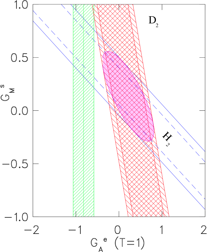
Figure 3: Allowed regions for the form factors $G_{M}^{s}$ and $-(1+R_{A}^{1})G_{A}\equiv G^{e}_{A}$ (in the notation of the figure), corresponding to the measurements of Refs. [91, 95] of the P–odd asymmetries for the proton ($H_{2}$, unshaded region) and for the deuteron ($D_{2}$, hatched region), respectively. The inner regions include statistical errors only, the outer ones include statistic and systematic uncertainties added in quadrature. The vertical shaded band corresponds to the calculated value of $-(1+R_{A}^{1})G_{A}$ using the theoretical estimate of Ref. [86] The isoscalar corrections $R_{A}^{0}$ are assumed to be the ones calculated in Ref. [86]. (Taken from Ref. [95])

The best–fit values of the form factors $G_{M}^{s}$ and $G_{A}^{e}$ at $Q^{2}=0.1$ GeV² are given by:

$$G_{M}^{s} =0.14\pm 0.29\,{\mathrm{stat}}\pm 0.31\,{\mathrm{syst}}\,,$$ (6.23)

$$G_{A}^{e}(T=1) =0.22\pm 0.45\,{\mathrm{stat}}\pm 0.39\,{\mathrm{syst}}\;.$$ (6.24)

In order to obtain from Eq.(6.23) the strange magnetic moment of the nucleon it is necessary to assume a $Q^{2}$–dependence of the strange form factor. In Ref. [95] a model proposed by Hemmert et al. [96], based on heavy baryon chiral perturbation theory, was used. For the strange magnetic moment the following value was then obtained

$$\mu_{s}=\left[0.01\pm 0.29\,{\mathrm{stat}}\pm 0.31\,{\mathrm{syst}}\pm 0.07\,{\mathrm{theor}}\right]\mu_{N}\,,$$ (6.25)

where the third error takes into account the theoretical uncertainty coming from different theoretical predictions. Thus, from the latest SAMPLE data it is impossible to draw any definite conclusion on the value of the strange magnetic moment of the nucleon.

Let us discuss now the value (6.24) of the axial constant. At $Q^{2}=0.1$ GeV², in Born approximation and assuming the usual axial dipole form factor, we have $G_{A}^{e}(T=1)=-1.071\pm 0.005$. Taking into account the radiative corrections calculated in Ref. [86], the following value of the form factor $G_{A}^{e}(T=1)$ was obtained [95]:

$$G_{A}^{e}(T=1)=-0.83\pm 0.26$$ (6.26)

This value corresponds to the vertical band in Fig. 3. Thus, the predicted value of $G_{A}^{e}(T=1)$ differs considerably from the experimental value, Eq. (6.24). One possible origin of this disagreement could be connected with a large anapole moment of the nucleon [95].

The surprising results which have been obtained in the SAMPLE experiments on the measurement of the P–odd asymmetry in $\vec{e}-p$ and $\vec{e}-d$ experiments require further theoretical efforts in the calculations of the radiative corrections and further experiments, which will allow to check these results (see also the recent review [97]). At present the SAMPLE collaboration has proposed a new experiment [98, 99] on the measurement of the P–odd asymmetry in the scattering on deuterium of polarized electrons with energy of $120$ MeV (thus lower than in the previous run). At this energy the asymmetry will be smaller, but the cross section will be significantly larger.

One final remark about the measurement of strange magnetic moment of the nucleon is in order: with the help of expression (2.9) for the electromagnetic current, we can present the Pauli form factors of proton and neutron in the following form:

$$\begin{array}[]{l}F_{2}^{p}=\frac{2}{3}F_{2}^{u}+\left(-\frac{1}{3}\right)F_{2}^{d}+\left(-\frac{1}{3}\right)F_{2}^{s}\\ F_{2}^{n}=\frac{2}{3}F_{2}^{d}+\left(-\frac{1}{3}\right)F_{2}^{u}+\left(-\frac{1}{3}\right)F_{2}^{s}\end{array}$$ (6.27)

where $F_{2}^{q}$ is the contribution of the $q$–quark ($q=u,d,s$) to the Pauli form factor of the proton. We have used in Eqs. (6.27) the isotopic SU(2) symmetry, from which it follows

$$\left(F_{2}^{u,d}\right)_{p}=\left(F_{2}^{d,u}\right)_{n}\,.$$

If we set $Q^{2}=0$ and take into account that $F_{2}^{p}(0)\equiv\kappa_{p}=1.79$, $F_{2}^{n}(0)\equiv\kappa_{n}=-1.91$, we obtain:

$$1.79 = \frac{2}{3}F_{2}^{u}(0)+\left(-\frac{1}{3}\right)F_{2}^{d}(0)+\left(-\frac{1}{3}\right)\mu_{s}\,,$$

$$-1.91 = \frac{2}{3}F_{2}^{d}(0)+\left(-\frac{1}{3}\right)F_{2}^{u}(0)+\left(-\frac{1}{3}\right)\mu_{s}$$

These relations can be combined to give:

$$\begin{array}[]{rcl}F_{2}^{u}(0)&=&\mu_{s}+1.67\\ F_{2}^{d}(0)&=&\mu_{s}-2.03\end{array}$$ (6.28)

Thus, the measurement of the strange magnetic moment of the nucleon will allow one to determine the contribution of the $u$ and $d$ quarks to the magnetic moments of proton and neutron. From (6.28) it follows that if $\mu_{s}>0.18$ then $F_{2}^{u}(0)\geq|F_{2}^{d}(0)|$, while in the case that $\mu_{s}<0.18$ the opposite inequality holds, $F_{2}^{u}(0)\leq|F_{2}^{d}(0)|$.

A new experiment on the measurement of P–odd asymmetry in elastic electron–proton scattering is going on at the Mainz Microtron Facility [100]. The energy of the electron beam in this experiment is of $855$ MeV. The scattered electrons are detected at a scattering angle of $35^{\circ}$ ($Q^{2}=0.227$ GeV²). The polarization of the electron beam is $80\%$. It is expected that the P–odd asymmetry will be measured with statistical accuracy of $3\%$ and systematic error of $4\%$. The combination of strange Dirac and Pauli form factors $F_{1}^{s}+0.13F_{2}^{s}$ at $Q^{2}=0.227$ GeV² will be determined from this experiment with accuracy of 0.02.

Finally, the G0 collaboration is measuring now the P–odd asymmetry in elastic electron–proton scattering at Jefferson Lab [101]. It is expected that from the data of this experiment the strange form factors will be determined with a few % accuracy at different values of $Q^{2}$ in the interval $0.1\leq Q^{2}\leq 1$ GeV².

Thus, in the nearest years we will have new information on the strange vector form factors of nucleon, an information which could have an important impact on our understanding of the nucleon structure and of strong interactions.

7 P–odd asymmetry in the elastic scattering of electrons on nuclei with $S=0$ $T=0$

In this Section we shall consider the elastic scattering of polarized electrons on nuclei with spin and isotopic spin equal to zero (like ⁴He, ¹²C, etc.). Interest for this case was raised in past works [102, 103, 104, 105].

$$\vec{e}+A\longrightarrow e+A$$ (7.1)

It is evident from the SU(2) isotopic invariance of strong interactions that in this case the matrix elements of the isovector currents $V^{3}_{\alpha}$ and $A^{3}_{\alpha}$ are equal to zero. Also the matrix element of the axial strange current $A^{s}_{\alpha}$ is equal to zero.

The matrix element of the process (7.1) is given by the general expression (5.2) in which $p$ ($p^{\prime}$) refers now to the initial (final) nucleus and, as before, $q=p^{\prime}-p$ and $Q^{2}=-q^{2}$. The process (7.1) can be represented by the same diagrams of Fig. 1, with the exchange of $\gamma$ and $Z^{0}$ between the electron and the nucleus.

For the matrix element of the electromagnetic current $J^{em}_{\alpha}$ we have now

$$\langle p^{\prime}|J^{em}_{\alpha}|p\rangle=\langle p^{\prime}|V^{0}_{\alpha}|p\rangle=(p+p^{\prime})_{\alpha}F(Q^{2})$$ (7.2)

where $V^{0}_{\alpha}$ is the isoscalar component of the electromagnetic current and $F(Q^{2})$ is the electromagnetic form factor of the nucleus (there is only one form factor in the case of a spin zero nucleus).

Similarly the nuclear matrix element of the NC reads

$$\langle p^{\prime}|J^{NC}_{\alpha}|p\rangle=\langle p^{\prime}|\left(-2\sin^{2}\theta_{W}J^{em}_{\alpha}-\frac{1}{2}V^{s}_{\alpha}\right)|p\rangle=(p+p^{\prime})_{\alpha}F^{NC}(Q^{2})$$ (7.3)

where

$$F^{NC}(Q^{2})=-2\sin^{2}\theta_{W}F(Q^{2})-\frac{1}{2}F^{s}(Q^{2})$$ (7.4)

and $F^{s}(Q^{2})$ is the strange form factor of the nucleus.

At $Q^{2}=0$ the form factor $F(Q^{2})$ is equal to the total charge of the nucleus

$$F(Q^{2}=0)=Z$$

while for the strange form factor we have, in the same limit,

$$F^{s}(Q^{2}=0)=0$$

(the net strangeness of the nucleus is equal to zero).

At small $Q^{2}$ we can expand the two form factors as follows:

$$F(Q^{2}) = Z\left(1-\frac{1}{6}\langle r^{2}\rangle Q^{2}+\dots\right)$$

$$F^{s}(Q^{2}) = -\frac{1}{6}\langle r_{s}^{2}\rangle Q^{2}+\dots$$

where $\langle r^{2}\rangle$ is the mean square of the electromagnetic radius of the nucleus and $\langle r^{2}_{s}\rangle$ is the mean square of the nuclear “strangeness radius”. Let us notice that in the impulse approximation, for nuclei with $N=Z$, we have

$$\frac{F^{s}(Q^{2})}{F(Q^{2})}=\frac{2G_{E}^{s}(Q^{2})}{G_{E}^{p}(Q^{2})+G_{E}^{n}(Q^{2})}\,.$$ (7.5)

The general expression for the cross section of the scattering of electrons with longitudinal polarization $\lambda$ on nuclei with zero spin can be obtained from Eq. (5) by setting $W^{I}_{\alpha\beta}(A)=0$. One gets then:

$$d\sigma_{\lambda}=\frac{4\alpha^{2}}{Q^{4}}\frac{M_{A}}{p\cdot k}\frac{1}{2}\left\{L^{\alpha\beta}W^{em}_{\alpha\beta}+\lambda\frac{G_{F}Q^{2}}{2\sqrt{2}\pi\alpha}g_{A}L^{\alpha\beta}W_{\alpha\beta}^{I}(V)\right\}\frac{d\vec{k^{\prime}}}{{k^{\prime}}^{0}}\,,$$ (7.6)

where $M_{A}$ is the mass of the nucleus and the tensors $W^{em}_{\alpha\beta}$ and $W^{I}_{\alpha\beta}(V)$ are given by Eqs. (5.13) and (5).

For a spin zero nucleus the tensors $W^{em}_{\alpha\beta}$ and $W^{I}_{\alpha\beta}(V)$ have the following general form

$$\begin{array}[]{l}W^{em}_{\alpha\beta}=\frac{\displaystyle{n_{\alpha}n_{\beta}}}{\displaystyle{4M_{A}^{2}}}\,W^{em}_{2}\\ W^{I}_{\alpha\beta}(V)=\frac{\displaystyle{n_{\alpha}n_{\beta}}}{\displaystyle{4M_{A}^{2}}}\,W^{I}_{2}\end{array}$$ (7.7)

where $n=p+p^{\prime}$. It is then easy to show that

$$\begin{array}[]{l}W^{em}_{2}=F^{2}(Q^{2})\,\delta\left(\nu-\frac{\displaystyle{Q^{2}}}{\displaystyle{2M_{A}}}\right)\,,\\ W^{I}_{2}=2F^{NC}(Q^{2})F(Q^{2})\,\delta\left(\nu-\frac{\displaystyle{Q^{2}}}{\displaystyle{2M_{A}}}\right)\end{array}$$ (7.8)

Here $\nu=E-E^{\prime}=p\cdot q/M_{A}$ is the energy transferred to the nucleus in the laboratory system.

By inserting (7.7) and (7.8) into (7.6), we obtain the following expression for the cross section of the scattering of electrons with longitudinal polarization $\lambda$ on spin zero nuclei:

$$\left(\frac{d\sigma}{d\Omega}\right)_{\lambda}=\left(\frac{d\sigma}{d\Omega}\right)_{0}(1+\lambda\mathcal{A})\,.$$ (7.9)

Here

$$\left(\frac{d\sigma}{d\Omega}\right)_{0}=\sigma_{Mott}F^{2}(Q^{2})$$ (7.10)

is the cross section for the scattering of unpolarized electrons on nuclei, $\sigma_{Mott}$ being the Mott cross section for a target nucleus of mass $M_{A}$:

$$\sigma_{Mott}=\frac{\alpha^{2}\cos^{2}(\theta/2)}{\displaystyle{4E^{2}\sin^{4}\frac{\theta}{2}\left(1+\frac{2E}{M_{A}}\sin^{2}\frac{\theta}{2}\right)}}\,.$$ (7.11)

In the above $\theta$ is the scattering angle and $E$ the initial energy of the electron in the laboratory system.

The P–odd asymmetry $\mathcal{A}$ is then given by [106]

$$\mathcal{A}(Q^{2}) = -\frac{G_{F}Q^{2}}{2\sqrt{2}\pi\alpha}\frac{F^{NC}(Q^{2})}{F(Q^{2})}=$$ (7.12)

$$= \frac{G_{F}Q^{2}}{2\sqrt{2}\pi\alpha}\left(2\sin^{2}\theta_{W}+\frac{F^{s}(Q^{2})}{2F(Q^{2})}\right)$$

As it is clearly seen from (7.12), the measured value of the asymmetry can be different from

$$\mathcal{A}_{(0)}(Q^{2})=\frac{G_{F}Q^{2}}{\sqrt{2}\pi\alpha}\sin^{2}\theta_{W}=8.309\times 10^{-5}\frac{Q^{2}}{\mathrm{GeV}^{2}}$$ (7.13)

only if the strange form factor $F^{s}(Q^{2})$ is different from zero. Important information on the strange form factor of the nucleus can be obtained from the investigation of the $Q^{2}$ dependence of the asymmetry: if the quantity $\mathcal{A}(Q^{2})/Q^{2}$ depends on $Q^{2}$, it would be the proof that the strange nuclear form factor is different from zero. Finally, should it occur that the P–odd asymmetry (7.12) is negative, it would imply that the strange form factor of the nucleus is large and negative.

From (7.12) it follows that the strange form factor of a nucleus with S=0 and T=0 is determined by quantities that can be experimentally measured. In fact we have

$$F^{s}(Q^{2})=2\sqrt{\frac{1}{\sigma_{Mott}}\left(\frac{d\sigma}{d\Omega}\right)_{0}}\left[\frac{2\sqrt{2}\pi\alpha}{G_{F}Q^{2}}\mathcal{A}(Q^{2})-2\sin^{2}\theta_{W}\right]\,.$$ (7.14)

An experiment on the measurement of the P–odd asymmetry in the elastic scattering of polarized electrons on ⁴He is under preparation at the Jefferson Lab [107]. The square of the momentum transfer in this experiment is expected to be $Q^{2}=0.6$ GeV². Two high resolution spectrometers will be employed. The target will be a circulating ⁴He gas system. Thus this experiment will be able to measure the above discussed strange form factor of a spin zero nucleus.

We like to mention, here, that the P–odd asymmetry in the elastic scattering of polarized electrons on nuclei represents an almost direct measurement of the Fourier transform of the neutron density, since the $Z^{0}$–boson preferentially couples to neutrons. Indeed for $0^{+}\to 0^{+}$ transitions, it is easy to show that the P–odd asymmetry can be expressed in the following form [108]:

$$\mathcal{A}=-\mathcal{A}_{0}\frac{1}{2}\left\{(1-4\sin^{2}\theta_{W})-\frac{\int d\vec{r}j_{0}(qr)\rho_{n}(\vec{r})}{\int d\vec{r}j_{0}(qr)\rho_{p}(\vec{r})}\right\}$$ (7.15)

which is valid both for isospin symmetric ($Z=N$) and asymmetric ($Z\neq N$) nuclei. In Eq. (7.15) $\rho_{n}$ ($\rho_{p}$) is the neutron (proton) density and $j_{0}(x)$ the spherical Bessel function of order zero. Taking into account the value of $\sin^{2}\theta_{W}$, the last term in the right hand side of Eq. (7.15) dominates the asymmetry and directly gives information on the neutron distribution. In fact the denominator coincides with the form factor $F(Q^{2})$, which can be measured independently [see Eq. (7.10)]. The Parity Radius Experiment (PREX) at the Jefferson Laboratory plans to measure the neutron radius $R_{n}$ in ²⁰⁸Pb through parity violating electron scattering [109]. The measurement of the neutron skin in a heavy nucleus ($R_{n}$ is generally assumed to be a few % larger that the proton radius) will have important implications on our knowledge of the structure of neutron stars, which are expected to have a solid, neutron–rich crust [110].

8 Inelastic Parity Violating (PV) electron scattering on nuclei

In addition to PV elastic electron scattering on proton, deuterium and $S=0,T=0$ nuclei, the P–odd asymmetry can be considered in the process of inelastic scattering of polarized electrons on nuclei. Several basic ideas motivate this investigation: the scattering on the single proton is not sufficient to determine the various unknown form factors which enter into the PV hadronic response; one is thus immediately led to consider also neutrons (namely deuterium) and more generally nuclei [82, 104, 111].

As we have discussed in the previous Section, the special case of elastic scattering on spin–zero, isospin-zero targets offers an unambiguous possibility to measure the strange form factor of the nucleus. However this type of investigation is confined to modest momentum transfers since the elastic nuclear form factors rapidly fall off with increasing momentum, with the exception of the very light nuclei. Therefore one would like to have additional, complementary information from other electron scattering measurements. One possibility is the inelastic excitation of discrete states in nuclei, but most probably the corresponding cross sections are not large enough to permit high precision information to be extracted.

A more promising case is the quasi–elastic (QE) scattering namely the inelastic scattering of electrons in the region of the so–called quasi–elastic peak [112]. This process roughly corresponds to “knocking” individual nucleons out of the nucleus without too much complication in the final nuclear state, in particular from final state interactions. QE scattering occurs for a given three–momentum transfer $q\equiv|{\vec{q}}\,|$, approximately at energy transfer $\omega=Q^{2}/(2M)$ The width of the peak is characterized by the Fermi momentum $p_{F}$ of the specific nucleus under study. In this kinematical region the cross sections are generally proportional to the number of nucleons in the nucleus, and thus are prominent features in the inelastic spectrum. One might then hope to perform high precision studies, which would complement work on parity–violating elastic electron scattering [82, 113].

The focuses of this investigation are multiple: on the one hand one wishes to understand the role played by the various single–nucleon form factors in the total asymmetry. By changing the kinematics ($q$, $\omega$ and the scattering angle $\theta$) and by adjusting $N$ and $Z$ through the choice of different targets, one can hope to alter the sensitivity of the asymmetry to the underlying form factors. Of course a precise study of nucleonic form factors from the scattering on nuclei is possible only if nuclear model uncertainties are well under control. On the other hand the measurement of the asymmetry in PV QE electron scattering brings into play new aspects of the nuclear many–body physics, namely the ones related to the nuclear response functions to NC probes. This might involve a sensitivity of the cross sections to specific dynamical aspects which cannot be revealed with the customary reactions employed in nuclear structure studies.

These issues were extensively discussed in Ref. [114] where PV quasi–elastic electron scattering was studied within the context of the relativistic Fermi gas (RFG). Let us consider the inclusive process in which a polarized electron with four–momentum $k$ and longitudinal polarization $\lambda$ is scattered through an angle $\theta$ to four–momentum $k^{\prime}$, exchanging a photon or a $Z^{0}$ to the target nucleus:

$$\vec{e}+A\longrightarrow e+A^{*}$$ (8.1)

We generically indicate with $A^{*}$ the final nucleus in an excited state, in which one (or more) nucleons are ejected. The leading order diagrams contributing to the amplitude of the process (8.1) are illustrated in Fig. 4. Only the final electron is detected and fixes the kinematics of the process.

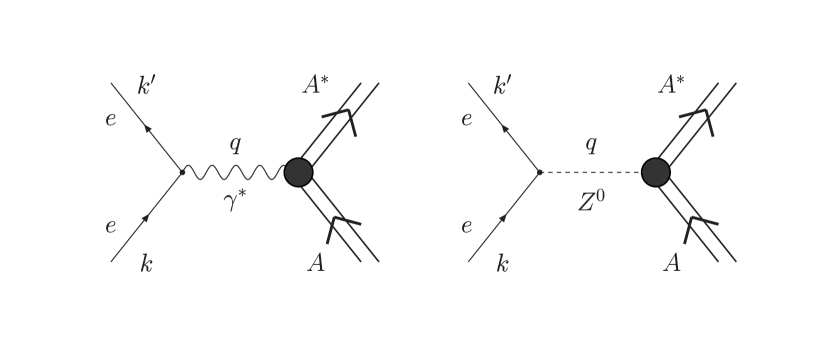
Figure 4: Single photon exchange and $Z^{0}$ exchange diagrams for electron scattering from nuclei.

The inclusive cross section for the scattering of polarized electrons on unpolarized nuclei can be written as:

$$d\sigma_{\lambda} =\frac{4\alpha^{2}}{Q^{4}}\frac{1}{2k^{0}}\left\{L^{\alpha\beta}W^{em}_{\alpha\beta}+\right.$$

$$\,\left.+\lambda\frac{G_{F}Q^{2}}{2\sqrt{2}\pi\alpha}\left[g_{V}L_{5}^{\alpha\beta}W^{I}_{\alpha\beta}(A)+g_{A}L^{\alpha\beta}W_{\alpha\beta}^{I}(V)\right]\right\}\frac{d\vec{k^{\prime}}}{{k^{\prime}}_{0}}\,,$$

where the leptonic tensor and pseudotensor, $L^{\alpha\beta}$ and $L_{5}^{\alpha\beta}$, are given in Eqs. (5.10) and (5.11). The hadronic (electromagnetic and interference) tensors are defined as:

$$W_{\alpha\beta}^{em} =\frac{3{\mathcal{N}}M^{2}}{4\pi p_{F}^{3}}\int\frac{d\vec{p}}{E_{p}}\frac{d\vec{p^{\prime}}}{E_{p^{\prime}}}\delta^{(4)}(p^{\prime}-p-q)\times$$ (8.3)

$$\qquad\times\theta(p_{F}-|{\vec{p}}\,|)\theta(|{\vec{p}}^{\,\prime}|-p_{F})\left(W_{\alpha\beta}^{em}\right)_{s.n.}\,,$$

and

$$W_{\alpha\beta}^{I}(V,A) =\frac{3{\mathcal{N}}M^{2}}{4\pi p_{F}^{3}}\int\frac{d\vec{p}}{E_{p}}\frac{d\vec{p^{\prime}}}{E_{p^{\prime}}}\,\delta^{(4)}(p^{\prime}-p-q)\times$$ (8.4)

$$\qquad\times\theta(p_{F}-|{\vec{p}}\,|)\theta(|{\vec{p}}^{\,\prime}|-p_{F})\left[W_{\alpha\beta}^{I}(V,A)\right]_{s.n.}\,.$$

In Eqs. (8.3) and (8.4) $E_{p}=\sqrt{\vec{p}^{2}+M^{2}}$ and the single–nucleon (s.n.) tensors are:

$$\left[W_{\alpha\beta}^{em}\right]_{s.n.}=-\tau G_{M}^{2}\left(g_{\alpha\beta}-\frac{q_{\alpha}q_{\beta}}{q^{2}}\right)+\frac{X_{\alpha}X_{\beta}}{M^{2}}\frac{\displaystyle{G_{E}^{2}+\tau G_{M}^{2}}}{\displaystyle{1+\tau}}$$ (8.5)

$$\left[W_{\alpha\beta}^{I}(V)\right]_{s.n.}=-2\tau G_{M}G_{M}^{NC}\left(g_{\alpha\beta}-\frac{q_{\alpha}q_{\beta}}{q^{2}}\right)+$$

$$\qquad\qquad\qquad\qquad+2\frac{X_{\alpha}X_{\beta}}{M^{2}}\frac{\displaystyle{G_{E}G_{E}^{NC}+\tau G_{M}G_{M}^{NC}}}{\displaystyle{1+\tau}}$$ (8.6)

$$\left[W_{\alpha\beta}^{I}(A)\right]_{s.n.}=\frac{i}{2M^{2}}\epsilon_{\alpha\beta\rho\sigma}p^{\rho}q^{\sigma}4G_{M}G_{A}^{NC}\,,$$ (8.7)

where $X_{\alpha}=p_{\alpha}-q_{\alpha}(q\cdot p)/q^{2}$. The expressions (8.3) and (8.4) for the nuclear hadronic tensors are obtained in the Impulse Approximation (IA), which amounts to consider the electron–nucleus interaction as an incoherent superposition of electron–nucleon scattering processes. Moreover the nucleus is described as a gas of non–interacting, relativistic nucleons, with momentum distribution $3{\mathcal{N}}/(4\pi p_{F}^{3})\theta(p_{F}-|\vec{p}\,|)$, $p_{F}$ being the Fermi momentum. In Eqs. (8.3) and (8.4) ${\mathcal{N}}=Z,N$ is the number of protons or neutrons in the nucleus and the function $\theta(|\vec{p^{\prime}}|-p_{F})$ ensures that the final nucleon is excited above the Fermi level (Pauli blocking effect). We also notice that the total cross section is obtained from the sum of the contributions from protons and neutrons, each of them being calculated by using the pertinent nucleonic form factors in the single–nucleon tensors (8.5)–(8.7).

From the above equations one can derive the expression for the double–differential (with respect to the energy, $k_{0}^{\prime}\equiv\epsilon^{\prime}$, and scattering angle, $\Omega$, of the final electron) inclusive cross section for the inelastic scattering of polarized electrons on nuclei. The sum of the cross sections for electrons with opposite polarization

$$\left(\frac{d^{2}\sigma}{d\Omega d\epsilon^{\prime}}\right)^{pc}=\frac{d^{2}\sigma_{+}}{d\Omega d\epsilon^{\prime}}+\frac{d^{2}\sigma_{-}}{d\Omega d\epsilon^{\prime}}=\sigma_{Mott}\left\{v_{L}R^{L}(q,\omega)+v_{T}R^{T}(q,\omega)\right\}$$ (8.8)

coincides with the inclusive, parity–conserving cross section for unpolarized electrons, which is obtained from the electromagnetic hadronic tensor only. Their difference, instead,

$$\left(\frac{d^{2}\sigma}{d\Omega d\epsilon^{\prime}}\right)^{pv}=\frac{d^{2}\sigma_{+}}{d\Omega d\epsilon^{\prime}}-\frac{d^{2}\sigma_{-}}{d\Omega d\epsilon^{\prime}}=$$

$$\,=-\sigma_{Mott}\frac{G_{F}Q^{2}}{2\sqrt{2}\pi\alpha}\left\{v_{L}R^{L}_{AV}(q,\omega)+v_{T}R^{T}_{AV}(q,\omega)+v_{T^{\prime}}R^{T^{\prime}}_{VA}(q,\omega)\right\}$$ (8.9)

denotes the parity–violating inclusive cross section, which is obtained from the interference hadronic tensors $W_{\alpha\beta}^{I}(V,A)$. It corresponds to the interference between the matrix elements for the exchange of one photon and the one for the exchange of a $Z^{0}$ boson. In Eqs.(8.8), (8.9) $\sigma_{Mott}$ is the Mott cross section and

$$v_{L} =\left(\frac{Q^{2}}{\vec{q}^{2}}\right)^{2},\qquad\quad v_{T}=\frac{1}{2}\frac{Q^{2}}{\vec{q}^{2}}+\tan^{2}\frac{1}{2}\theta$$ (8.10)

$$v_{T^{\prime}} =\sqrt{\frac{Q^{2}}{\vec{q}^{2}}+\tan^{2}\frac{1}{2}\theta}\,\tan\frac{1}{2}\theta$$ (8.11)

are lepton kinematical factors.

The functions $R^{L(T)}(q,\omega)$ ($q=|\vec{q}|$) are the longitudinal (transverse) electromagnetic nuclear response functions, which are given by:

$$R^{L}(q,\omega) =W_{00}^{em},$$ (8.12)

$$R^{T}(q,\omega) =W_{11}^{em}+W_{22}^{em},$$ (8.13)

the direction of the three–momentum transfer $\vec{q}$ being assumed as $z$–axis. The corresponding parity–violating nuclear response functions are defined as:

$$R^{L}_{AV}(q,\omega) =g_{A}W_{00}^{I}(V)\,,$$ (8.14)

$$R^{T}_{AV}(q,\omega) =g_{A}\left[W_{11}^{I}(V)+W_{22}^{I}(V)\right]\,,$$ (8.15)

$$R^{T^{\prime}}_{VA}(q,\omega) =ig_{V}W_{12}^{I}(A)\,.$$ (8.16)

By measuring the cross sections for the scattering of electrons with both polarizations one can determine the asymmetry:

$${\mathcal{A}}= \left({\displaystyle{\frac{d^{2}\sigma_{+}}{d\Omega d\epsilon^{\prime}}-\frac{d^{2}\sigma_{-}}{d\Omega d\epsilon^{\prime}}}}\right)/\left({\displaystyle{\frac{d^{2}\sigma_{+}}{d\Omega d\epsilon^{\prime}}+\frac{d^{2}\sigma_{-}}{d\Omega d\epsilon^{\prime}}}}\right)$$ (8.17)

$$=\mathcal{A}_{0}\,\frac{v_{L}R^{L}_{AV}(q,\omega)+v_{T}R^{T}_{AV}(q,\omega)+v_{T^{\prime}}R^{T^{\prime}}_{VA}(q,\omega)}{v_{L}R^{L}(q,\omega)+v_{T}R^{T}(q,\omega)}$$

where $\mathcal{A}_{0}$ is defined in Eq. (5.8).

Within the RFG model the above defined nuclear response functions can be analytically evaluated. By performing the integrals over $\vec{p}$ one obtains:

$$R^{L,T}(q,\omega) =R_{0}(q,\omega)U^{L,T}(q,\omega)$$ (8.18)

$$R^{L,T}_{AV}(q,\omega) =R_{0}(q,\omega)g_{A}U^{L,T}_{AV}(q,\omega)$$ (8.19)

$$R^{T^{\prime}}_{VA}(q,\omega) =R_{0}(q,\omega)g_{V}U^{T^{\prime}}_{VA}(q,\omega)$$ (8.20)

where

$$R_{0}(q,\omega)=\frac{3{\mathcal{N}}M^{2}}{2qp_{F}^{3}}\left(E_{F}-\Gamma\right)\theta\left(E_{F}-\Gamma\right)\,.$$ (8.21)

In Eq. (8.21) $E_{F}=\sqrt{p_{F}^{2}+M^{2}}$ is the Fermi energy and

$$\Gamma(q,\omega)=\max\left\{(E_{F}-\omega),\,\,\frac{1}{2}\left(q\sqrt{1+\frac{1}{\tau}}-\omega\right)\right\}\,.$$

Two regimes exist: (i) $q<2p_{F}$, where $\Gamma=E_{F}-\omega$ and Pauli blocking occurs; and (ii) $q\geq 2p_{F}$, where $\Gamma=\frac{1}{2}\left(q\sqrt{1+\frac{1}{\tau}}-\omega\right)$ and the responses are not Pauli blocked. The remaining dependence on $q$ and $\omega$ in Eqs. (8.18)–(8.20) is contained in the reduced responses:

$$U^{L}(q,\omega) = \frac{q^{2}}{Q^{2}}\left\{G_{E}^{2}+\frac{1}{1+\tau}\left(G_{E}^{2}+\tau G_{M}^{2}\right)\Delta\right\}$$

$$U^{T}(q,\omega) = 2\,\tau G_{M}^{2}+\frac{1}{1+\tau}\left(G_{E}^{2}+\tau G_{M}^{2}\right)\Delta$$

$$U^{L}_{AV}(q,\omega) = 2\,\frac{q^{2}}{Q^{2}}\left\{G_{E}G_{E}^{NC}+\frac{1}{1+\tau}\left(G_{E}G_{E}^{NC}+\tau G_{M}G_{M}^{NC}\right)\Delta\right\}$$ (8.22)

$$U^{T}_{AV}(q,\omega) = 4\,\tau G_{M}G_{M}^{NC}+\frac{2}{1+\tau}\left(G_{E}G_{E}^{NC}+\tau G_{M}G_{M}^{NC}\right)\Delta$$

$$U^{T^{\prime}}_{VA}(q,\omega) = \sqrt{\tau(1+\tau)}\,4\,G_{M}G_{A}^{NC}(1+\Delta^{\prime})\,.$$

Here the following functions of $q$, $\omega$ and $p_{F}$ have been introduced:

$$\Delta=\frac{Q^{2}}{q^{2}}\left\{\frac{1}{3M^{2}}\left(E_{F}^{2}+E_{F}\Gamma+\Gamma^{2}\right)+\frac{\omega}{2M^{2}}\left(E_{F}+\Gamma\right)+\frac{\omega^{2}}{4M^{2}}\right\}+$$

$$\qquad\qquad\qquad-(1+\tau)$$ (8.23)

$$\Delta^{\prime}=\frac{1}{2q}\sqrt{\frac{\tau}{1+\tau}}\left\{E_{F}+\Gamma+\omega\right\}-1$$ (8.24)

In most kinematical situations the quantities $\Delta$ and $\Delta^{\prime}$ are small and their effect on the P–odd asymmetry is negligible, below the percent. It is interesting to notice that by setting $\Delta=\Delta^{\prime}=0$ the presence of the nuclear medium in the response functions (8.18)–(8.20) is felt through the function $R_{0}(q,\omega)$ only. The latter obviously cancels in the expression (8.17) of the asymmetry, thus leading to the same combination of form factors which was obtained in the case of elastic electron–proton scattering. This fact endures the possibility of using the measurements of quasi–elastic cross sections in the scattering of polarized electrons on nuclei to extract information on the strange form factors of the nucleon. Indeed, as discussed in Ref. [114], the nuclear physics dependence of the P–odd asymmetry which emerges from the calculations in the RFG model is rather weak.

Typical results for ¹²C are shown in Fig. 5. The Fermi momentum is taken to be $p_{F}=225$ MeV and the strange form factors are set to zero. In the upper panels the two electromagnetic response functions ($R^{L}$, $R^{T}$) are displayed as a function of energy transfer $\omega$, for three typical 3–momentum transfers, $q=0.3,\,0.5$ and $2$ GeV. The intermediate panels show the corresponding parity violating responses $R^{L}_{AV}$, $R^{T}_{AV}$ and $R^{T^{\prime}}_{VA}$. Quasi–elastic scattering allows one to explore these quantities (as well as the P–odd asymmetry) in different kinematical ranges. The $Q^{2}$ values corresponding to the peak of the responses ($\omega=Q^{2}/2M$) are 0.09, 0.24 and 2.4 GeV², respectively, but for each case a range of different $Q^{2}$ is explored (for example $1.9\leq Q^{2}\leq 2.9$ GeV² in the right panels), thus showing one of the advantages of this investigation. Once these response functions are multiplied by the (angle dependent) lepton kinematical factors (8.10), (8.11) and combined as in Eq. (8.17), one obtains the asymmetry shown in the lower panels of Fig. 5. It ranges from a few $\times 10^{-6}$ at forward angle and low $q$ to a few $\times 10^{-4}$ for a broad range of angles at $q=2$ GeV.

Figure 5: Relativistic Fermi gas response functions and asymmetry for ¹²C at different values of $q$, shown as a function of $\omega$. The location of $\omega=Q^{2}/(2M)$ is indicated by the arrows. Further explanations in the text (Taken from Ref. [114]).

Further, one can examine the sensitivity of the P–odd asymmetry to the nucleon strange and non–strange form factors . At backward scattering angles $v_{L}/v_{T}\to 0$, $v_{T^{\prime}}/v_{T}\to 1$ and the terms containing magnetic and axial form factors dominate (in spite of the $g_{V}$ factor which penalizes the interference with the axial nuclear current). In Ref. [114] the electromagnetic form factors of the proton were parameterized with the usual dipole form, with a cutoff mass $M_{V}=843$ MeV; for the neutron the following form factors were used:

$$G_{M}^{n}(Q^{2}) =\frac{\rho_{M_{n}}\mu_{n}}{\displaystyle{\left(1+\frac{Q^{2}}{M_{V}^{2}}\right)^{2}}},\qquad$$ (8.25)

$$G_{E}^{n}(Q^{2}) =\frac{-\mu_{n}\tau}{\displaystyle{\left(1+\frac{Q^{2}}{M_{V}^{2}}\right)^{2}(1+\lambda_{n}\tau)}}\,,$$ (8.26)

where the Galster [115, 116] parameterization for $G_{E}^{n}$ was assumed, with $\mu_{n}=-1.1913$ and $\lambda_{n}=5.6$. The standard value of the parameter $\rho_{M_{n}}$ is unity; it accounts for possible deviations as in Eq. (6.4). The axial isovector form factor was parameterized as

$$G_{A}(Q^{2})=\frac{g_{A}}{\displaystyle{\left(1+\frac{Q^{2}}{M_{A}^{2}}\right)^{2}}}\,,$$ (8.27)

with $M_{A}=1$ GeV. For the strange form factors the following parameterization was adopted:

$$G_{E}^{s}(Q^{2}) = \frac{\rho_{s}\tau}{\displaystyle{\left(1+\frac{Q^{2}}{M_{V}^{2}}\right)^{2}(1+\lambda_{E}^{s}\tau)}}\,,$$ (8.28)

$$G_{M}^{s}(Q^{2}) = \frac{\mu_{s}}{\displaystyle{\left(1+\frac{Q^{2}}{M_{V}^{2}}\right)^{2}(1+\lambda_{M}^{s}\tau)}}\,,$$ (8.29)

$$G_{A}^{s}(Q^{2}) = \frac{g_{A}^{s}\tau}{\displaystyle{\left(1+\frac{Q^{2}}{M_{A}^{2}}\right)^{2}(1+\lambda_{A}^{s}\tau)}}\,,$$ (8.30)

where the second factor in the denominators accounts for possible deviations of the high–$\tau$ dipole fall–off. In Ref. [114] the values $\lambda_{E}^{s}=\lambda_{n}$, $\lambda_{M}^{s}=\lambda_{A}^{s}=0$ were used.

The correlations between different parameters used in modeling the form factors were examined by looking at the dependence of one parameter from a second one (all the remaining ones being fixed) keeping the P–odd asymmetry constant. In Fig. 6 a few examples of these correlation plots are shown for ¹²C at $q=500$ MeV, $\omega=Q^{2}/(2M)$ and $\theta=150^{\circ}$: the lines marked $0\%$ correspond to a (constant) value of $\mathcal{A}$ which is obtained starting with the “standard” values (e.g. $g_{A}=1.26$, $\rho_{s}=0$ in the upper right panel). Lines marked $+1\%$ ($-1\%$) have asymmetries $1.01\mathcal{A}$ ($0.99\mathcal{A}$), with a corresponding meaning for the lines marked $\pm 5\%$. From these curves one observes, for example, that at this particular choice of kinematics, a $\pm 1\%$ determination of the asymmetry would permit a $\pm 5.6\%$ determination of $g_{A}$ if everything else were known (we refer the reader to the above discussion on the uncertainties on this parameter due, e.g., to radiative corrections). A $\pm 5\%$ determination of $\mathcal{A}$ likewise would translate into a $\pm 28\%$ uncertainty in $g_{A}$. In fact, there are uncertainties in the other parameters which enter into the problem and in the nuclear model itself.

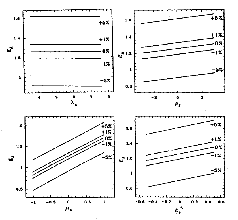
Figure 6: Correlation plots for ¹²C at $q=500$ MeV, $\omega=Q^{2}/(2M)$ and $\theta=150^{\circ}$. The asymmetry is constant for any pairs of parameters corresponding to the line marked $0\%$. For lines marked $\pm 1\%$ ($\pm 5\%$) the asymmetry remains constant at values $1\%$ ($5\%$) larger or smaller than that obtained with the canonical choice of parameters. The panels show correlations of $g_{A}$ with $\lambda_{n}$, $\rho_{s}$, $\mu_{s}$ and $g_{A}^{s}$. Further explanations in the text (Taken from Ref. [114]).

The parameter $\lambda_{n}$ characterizes the high–$\tau$ fall–off of the electric form factor of the neutron, $G_{E}^{n}$: we see from the left upper panel of Fig. 6 that, if the latter will be determined in future experiments to $\pm 10\%$, this only translates into a $\pm 0.6\%$ uncertainty in $g_{A}$. Obviously this relatively minor effect is due the backward kinematics, which suppresses the longitudinal contributions. The left lower panel of Fig. 6 shows the correlation between $g_{A}$ and the strength of $G_{M}^{s}$, $\mu_{s}$: if this parameter goes from 0 to $-1$, (from 0 to 1) then $g_{A}$ would decrease (increase) by $34.7\%$. This correlation is rather important: for example if $g_{A}$ were known to $\pm 10\%$, then $\mu_{s}$ would be constrained to $\pm 0.29$. Finally the right lower panel shows a non–negligible correlation between $g_{A}$ and $g_{A}^{s}$.

One should also notice, here, the potentialities offered by the use of different nuclear targets. Indeed the measurement of $\mathcal{A}$ in inelastic electron–nucleus scattering can give information not only on the strange nucleon form factors, but also on the non–strange parts of the weak neutral form factors of the nucleon. This can be achieved by filtering the latter with a suitable choice of $Z$ and $N$, such that, for example, it enhances the isovector contributions to the nuclear response and eventually cancels the isoscalar ones.

As an illustration, let us consider the product $G_{M}G_{M}^{NC}$ in $U^{T}_{AV}$ or $G_{M}G_{A}^{NC}$ in $U^{T^{\prime}}_{VA}$, in Eqs. (8.22): in a $(Z,N)$ nucleus both $G_{M}^{s}$ and $G_{A}^{s}$ enter $\mathcal{A}$ multiplied by the combination $ZG_{M}^{p}+NG_{M}^{n}$, whereas the non–strange contributions (e.g. the isovector part of $G_{A}^{NC}$) enter with $ZG_{M}^{p}-NG_{M}^{n}$. Hence the ratio of the strange to the non–strange transverse pieces is $(ZG_{M}^{p}+NG_{M}^{n})/(ZG_{M}^{p}-NG_{M}^{n})$. This ratio is 1 for the proton, 0.187 for a $Z=N$ nucleus and can be further reduced to be nearly zero by choosing a nucleus whose $N/Z$ ratio is very close to $-\mu_{p}/\mu_{n}$. The case of tungsten (¹⁸⁴W), having advantages for high luminosity experiments, gives a ratio of $-0.009$. In Fig. 7 correlation plots are shown for $q=500$ MeV and $\theta=150^{\circ}$; the results for ¹²C and ¹⁸⁴W are obtained by integrating over the entire quasi–elastic response region, although there is no significative difference between the peak asymmetry and the integrated result. In (a) a significative interplay appears between $g_{A}$ and $\rho_{M_{n}}$, more pronounced in H than in C and W, but not negligible even in the last case. In (b) and (c) instead, it is clearly shown that no correlation exists in W between $g_{A}$ and the strangeness parameters $\mu_{s}$ and $g_{A}^{s}$: thus an $N>Z$ nucleus such as tungsten appears to have advantages for the determination of $G_{A}$ in backward–angle scattering.

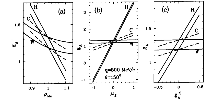
Figure 7: Correlation plots as in Fig. 6, showing $g_{A}$ correlated with (a) $\rho_{M_{n}}$, (b) $\mu_{s}$ and (c) $g_{A}^{s}$, for $q=500$ MeV and $\theta=150^{\circ}$. Three cases are shown: elastic scattering from hydrogen (labelled H) and quasi–elastic scattering from carbon (C) and tungsten (W). Only the $\pm 1\%$ contour lines are shown. For tungsten two different Fermi momenta are used: $p_{F}^{p}=250$ MeV for protons and $p_{F}^{n}=285$ MeV for neutrons. (Taken from Ref. [114]).

A special case with $N=Z$ is the deuteron, which we have already mentioned in Section 6, discussing the SAMPLE experiment at MIT/Bates. In the kinematic region around the QE peak the P-odd asymmetry for the deuteron can be evaluated in the so–called “static” approximation, in which the contributions to the cross sections of protons and neutrons at rest are summed incoherently [117]:

$$\left(\frac{\mathcal{A}}{\mathcal{A}_{0}}\right)_{d}=2\,\left\{g_{A}\left[v_{L}\frac{q^{2}}{2Q^{2}}\left(G_{E}^{p}G_{E}^{NC;p}+G_{E}^{n}G_{E}^{NC;n}\right)\right.\right.+$$

$$\left.+v_{T}\;\tau\left(G_{M}^{p}G_{M}^{NC;p}+G_{M}^{n}G_{M}^{NC;n}\right)\right]+$$

$$+g_{V}\left.\left[v_{T}\sqrt{\tau(1+\tau)}\left(G_{M}^{p}G_{A}^{NC;p}+G_{M}^{n}G_{A}^{NC;n}\right)\right]\right\}\times$$

$$\times\left[v_{L}\frac{q^{2}}{2Q^{2}}\left(\left(G_{E}^{p}\right)^{2}+\left(G_{E}^{n}\right)^{2}\right)+v_{T}\left[\tau\left((G_{M}^{p})^{2}+(G_{M}^{n})^{2}\right)\right]\right]^{-1}\;.$$ (8.31)

This formula can be obtained from the RFG , setting the terms $\Delta$ and $\Delta^{\prime}$ in Eqs. (8.22) to zero and taking $N=Z=1$. The dependence of the P-odd asymmetry on the deuteron structure was studied in Ref. [117], under different conditions. The authors concluded that in the kinematical region around the QE peak deviations from the static model are within 1 or 2 %. A more recent study of the deuteron structure effects in $A_{d}$ for the specific kinematic conditions of the SAMPLE experiment can be found in [118]. To get a flavor of the general sensitivity of $\mathcal{A}_{d}$ to the single nucleon form factors one can consider the transverse contributions in Eq. (8.31), which are dominant at large scattering angles, as in the SAMPLE experiment. As already stated for the general case $N=Z$, the strange form factors $G_{M}^{s}$ and $G_{A}^{s}$ enter the transverse contributions to the asymmetry multiplied by the combination $G_{M}^{p}+G_{M}^{n}$ and are suppressed by a factor $\simeq 0.187$ with respect to the contribution coming from the isovector axial form factor $G_{A}$, which is multiplied by $G_{M}^{p}-G_{M}^{n}$.

As a final issue in this Section let us consider forward–angle scattering: at small $\theta$ and fixed $q$, $\omega$ it is $v_{L}/v_{T}\to 2Q^{2}/q^{2}$ and $v_{T^{\prime}}/v_{T}\to 0$, so that the contribution of the response $R_{T^{\prime}}(q,\omega)$ is suppressed. In this situation considerable sensitivity of the asymmetry to the electric strange form factor can be achieved. In Fig. 8 the correlation plot of $\rho_{s}$ versus $\mu_{s}$ is shown for ¹²C at $q=500$ MeV and $\theta=10^{\circ}$.

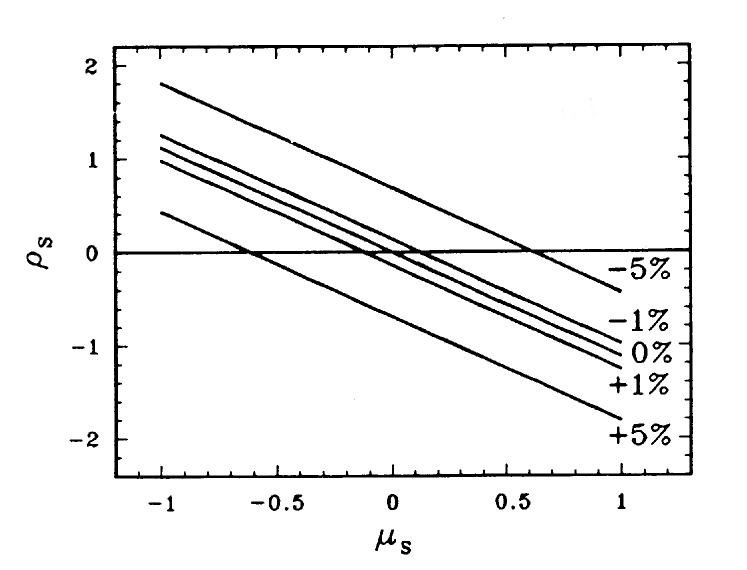
Figure 8: Correlation plots as in Fig. 6, showing $\rho_{s}$ correlated with $\mu_{s}$, for $q=500$ MeV, $\omega=Q^{2}/(2M)$ and $\theta=10^{\circ}$. (Taken from Ref. [114]).

From all the above consideration, quasi–elastic scattering of polarized electrons on nuclei can be considered, with appropriate choices of the kinematical conditions, as a useful tool to determine the strange form factors of the nucleon; it can also provide important information on the non–strange components of various nucleonic form factors , which are still waiting for a precise determination. Although it goes outside the scopes of the present review, we also mention that the measurement of parity–violating nuclear response functions would open new and interesting possibilities to explore the nuclear dynamics as viewed by weak neutral probes and to test nuclear models in the domain of medium–high excitation energy [119, 120].

9 Elastic NC scattering of neutrinos (antineutrinos) on the nucleon

Direct information on the strange form factors of the nucleon can be obtained from the investigation of the NC processes [121, 122]

$$\nu_{\mu}(\overline{\nu}_{\mu})+N\longrightarrow\nu_{\mu}(\overline{\nu}_{\mu})+N$$ (9.1)

The amplitude for the process of neutrino (antineutrino) scattering is given by the following expression

$$\langle f|S|i\rangle=\mp\frac{G_{F}}{\sqrt{2}}\overline{u}(k^{\prime})\gamma^{\alpha}\left(1\mp\gamma_{5}\right)u(k)\langle p^{\prime}|J^{NC}_{\alpha}|p\rangle(2\pi)^{8}\delta^{(4)}(p^{\prime}-p-q)$$ (9.2)

where $k$ and $k^{\prime}$ are the momenta of the initial and final neutrino (antineutrino), $p$ and $p^{\prime}$ the momenta of the initial and final nucleon, $q=k-k^{\prime}$ and

$$J_{\alpha}^{NC}=V_{\alpha}^{NC}-A_{\alpha}^{NC}$$

is the hadronic neutral current in the Heisenberg representation.

The matrix elements of the vector and axial NC are given in the Standard Model by the expressions (4.19) and (4.20). The cross sections of the processes (9.1) turn out to be

$$d\sigma_{\nu(\overline{\nu})}=\frac{G_{F}^{2}}{(2\pi)^{2}}\frac{M}{p\cdot k}\left\{L^{\alpha\beta}(k,k^{\prime})\mp L_{5}^{\alpha\beta}(k,k^{\prime})\right\}W^{NC}_{\alpha\beta}(p,q)\frac{d\vec{k^{\prime}}}{k^{\prime}_{0}}\,,$$ (9.3)

where

$$W_{\alpha\beta}^{NC}(p,q)=\frac{1}{2M}\sum\int\langle p^{\prime}|J^{NC}_{\alpha}|p\rangle\langle p|J^{NC}_{\beta}|p^{\prime}\rangle\delta^{(4)}(p^{\prime}-p-q)\frac{d\vec{p^{\prime}}}{2p^{\prime}_{0}}$$ (9.4)

while the tensor $L^{\alpha\beta}(k,k^{\prime})$ and pseudotensor $L^{\alpha\beta}_{5}(k,k^{\prime})$ are given by (5.10) and (5.11), respectively.

It is evident that $W_{\alpha\beta}^{NC}$ has the following structure

$$W^{NC}_{\alpha\beta}=W_{\alpha\beta}^{VV+AA}-W_{\alpha\beta}^{VA}$$ (9.5)

where, with obvious notation, the tensor$W_{\alpha\beta}^{VV+AA}$ is due to the contribution of the vector–vector and axial–axial NC, whereas the pseudotensor $W_{\alpha\beta}^{VA}$ is due to the interference of the vector and axial NC.

After performing the traces over spin states, they become ($\tau=Q^{2}/4M^{2}$, $n=p+p^{\prime}$):

$$W_{\alpha\beta}^{VV+AA}=\left\{-\left[\tau\left(G_{M}^{NC}\right)^{2}+\left(1+\tau\right)\left(G_{A}^{NC}\right)^{2}\right]\left(g_{\alpha\beta}-\frac{q_{\alpha}q_{\beta}}{q^{2}}\right)\right.+$$

$$\qquad\quad+\left[\frac{\left(G_{E}^{NC}\right)^{2}+\tau\left(G_{M}^{NC}\right)^{2}}{1+\tau}+\left(G_{A}^{NC}\right)^{2}\right]\frac{n_{\alpha}n_{\beta}}{4M^{2}}$$

$$\qquad\qquad\left.-\frac{q_{\alpha}q_{\beta}}{q^{2}}\left(G_{A}^{NC}\right)^{2}\right\}\delta\left(\nu-\frac{Q^{2}}{2M}\right)$$ (9.6)

and

$$W^{VA}_{\alpha\beta}=\frac{i}{M^{2}}\epsilon_{\alpha\beta\rho\sigma}p^{\rho}{p^{\prime}}^{\sigma}G_{M}^{NC}G_{A}^{NC}\delta\left(\nu-\frac{Q^{2}}{2M}\right)\,,$$ (9.7)

respectively.

Taking into account that

$$\frac{d\vec{k^{\prime}}}{{k^{\prime}}_{0}}=\pi\frac{M}{p\cdot k}\,dQ^{2}d\nu\,,$$ (9.8)

from Eqs. (9.3), (9.6) and (9.7) we obtain, correspondingly, the following expressions for the differential cross sections of the processes (9.1):

$$\left(\frac{d\sigma}{dQ^{2}}\right)^{NC}_{\nu(\overline{\nu})}=$$

$$\qquad=\frac{G_{F}^{2}}{2\pi}\left[\frac{1}{2}y^{2}(G_{M}^{NC})^{2}+\left(1-y-\frac{M}{2E}y\right)\frac{\displaystyle{(G_{E}^{NC})^{2}+\frac{E}{2M}y(G_{M}^{NC})^{2}}}{\displaystyle{1+\frac{E}{2M}y}}\right.$$

$$\qquad\left.+\left(\frac{1}{2}y^{2}+1-y+\frac{M}{2E}y\right)(G_{A}^{NC})^{2}\pm 2y\left(1-\frac{1}{2}y\right)G_{M}^{NC}G_{A}^{NC}\right]\,.$$ (9.9)

Here

$$y=\frac{p\cdot q}{p\cdot k}=\frac{Q^{2}}{2p\cdot k}$$ (9.10)

and $E$ is the energy of neutrino (antineutrino) in the laboratory system.

In order to obtain information on the strange form factors of the nucleon from the investigation of the processes (9.1) it is necessary to know the axial CC form factor $G_{A}$ [see relation (4.22)]. The latter can be determined by investigating the quasi–elastic processes

$$\begin{array}[]{l}\nu_{\mu}+n\longrightarrow\mu^{-}+p\,,\\ \overline{\nu}_{\mu}+p\longrightarrow\mu^{+}+n\,.\end{array}$$ (9.11)

The amplitudes of these processes are given, respectively, by the expressions

$$\langle f|S|i\rangle = -i\frac{G_{F}}{\sqrt{2}}\overline{u}(k^{\prime})\gamma^{\alpha}(1-\gamma_{5})u(k)\langle p^{\prime}|J_{\alpha}^{CC}|p\rangle(2\pi)^{4}\delta^{(4)}(p^{\prime}-p-q)$$ (9.12)

$$\langle f|S|i\rangle = i\frac{G_{F}}{\sqrt{2}}\overline{u}(k^{\prime})\gamma^{\alpha}(1+\gamma_{5})u(k)\langle p^{\prime}|{J_{\alpha}^{CC}}^{\dagger}|p\rangle(2\pi)^{4}\delta^{(4)}(p^{\prime}-p-q)$$ (9.13)

where $k$ and $k^{\prime}$ are the momenta of the initial $\nu_{\mu}$ ($\bar{\nu}_{\mu}$) and final $\mu^{-}$ ($\mu^{+}$) lepton, $p$ is the momentum of the initial $n$ ($p$) and $p^{\prime}$ the momentum of the final $p$ ($n$). The Heisenberg vector and axial charged currents are the “plus”–components of the isovectors $V_{\alpha}^{i}$ and $A_{\alpha}^{i}$ [see Eq. (3.24)].

In Section 3 we have considered the one–nucleon matrix elements of the axial current $A_{\alpha}^{1+i2}$. Let us discuss now the matrix element of the vector current $V_{\alpha}^{1+i2}$. Due to isotopic invariance of the strong interactions the vector current $V_{\alpha}^{i}$ is conserved (Conserved Vector Current, CVC) [123]:

$$\partial^{\alpha}V_{\alpha}^{i}=0.$$

Thus the matrix element of the vector current satisfies the condition

$$\left(p^{\prime}-p\right)^{\alpha}\,{{}_{p}\langle}p^{\prime}|V^{1+i2}_{\alpha}|p\rangle_{n}=0$$ (9.14)

and has the following general form

$${{}_{p}\langle}p^{\prime}|V^{1+i2}_{\alpha}|p\rangle_{n}=\overline{u}(p^{\prime})\left[\gamma_{\alpha}F_{1}^{CC}(Q^{2})+\frac{i}{2M}\sigma_{\alpha\beta}q^{\beta}F_{2}^{CC}(Q^{2})\right]u(p)$$ (9.15)

where $F_{1,2}^{CC}(Q^{2})$ are CC form factors. The corresponding Sachs CC form factors are given by

$$G_{M}^{CC}(Q^{2}) = F_{1}^{CC}(Q^{2})+F_{2}^{CC}(Q^{2})$$ (9.16)

$$G_{E}^{CC}(Q^{2}) = F_{1}^{CC}(Q^{2})-\frac{Q^{2}}{4M^{2}}F_{2}^{CC}(Q^{2})$$ (9.17)

An important property of the isovector current $V_{\alpha}^{i}$ is given by its commutation relation with the isospin operator

$$\left[I_{k},V^{j}_{\alpha}\right]=i\epsilon_{kj\ell}V_{\alpha}^{\ell}$$ (9.18)

where $I_{k}$ is the total isotopic spin operator. From Eq. (9.18) it follows that

$$V_{\alpha}^{1+i2}=\left[V_{\alpha}^{3},I_{1+i2}\right]\,.$$ (9.19)

Taking into account the charge symmetry of strong interactions, from (9.19) the following relations hold:

$${{}_{p}\langle}p^{\prime}|V^{1+i2}_{\alpha}|p\rangle_{n}={{}_{n}\langle}p^{\prime}|V^{1-i2}_{\alpha}|p\rangle_{p}={{}_{p}\langle}p^{\prime}|J^{em}_{\alpha}|p\rangle_{p}-{{}_{n}\langle}p^{\prime}|J^{em}_{\alpha}|p\rangle_{n}\,.$$

Let us notice that in the derivation of these relations we have used the expression (2.17) for the e.m. current. Thus the CC vector form factors are connected with the electromagnetic form factors of proton and neutron by:

$$G_{M}^{CC}(Q^{2}) = G_{M}^{p}(Q^{2})-G_{M}^{n}(Q^{2})$$ (9.20)

$$G_{E}^{CC}(Q^{2}) = G_{E}^{p}(Q^{2})-G_{E}^{n}(Q^{2})$$ (9.21)

The cross sections of the processes (9.11) are given by the expression (9.3) in which $W_{\alpha\beta}^{NC}$ have to be replaced by

$$W_{\alpha\beta}^{CC}(p,q)=\frac{1}{2M}\sum\int\langle p^{\prime}|J^{CC}_{\alpha}|p\rangle\langle p|{J^{CC}_{\beta}}^{\dagger}|p^{\prime}\rangle\delta^{(4)}(p^{\prime}-p-q)\frac{d\vec{p^{\prime}}}{2p^{\prime}_{0}}$$ (9.22)

It is obvious that in order to obtain the cross sections of the quasi–elastic processes (9.11) it is necessary to replace the NC form factors in the expression (9.9) by the CC ones (we are neglecting the muon mass). One gets:

$$\left(\frac{d\sigma}{dQ^{2}}\right)^{CC}_{\nu(\overline{\nu})}=$$ (9.23)

$$\qquad=\frac{G_{F}^{2}}{2\pi}\left[\frac{1}{2}y^{2}(G_{M}^{CC})^{2}+\left(1-y-\frac{M}{2E}y\right)\frac{\displaystyle{(G_{E}^{CC})^{2}+\frac{E}{2M}y(G_{M}^{CC})^{2}}}{\displaystyle{1+\frac{E}{2M}y}}\right.+$$

$$\qquad\qquad\left.+\left(\frac{1}{2}y^{2}+1-y+\frac{M}{2E}y\right)(G_{A})^{2}\pm 2y\left(1-\frac{1}{2}y\right)G_{M}^{CC}G_{A}\right]\,.$$

The most detailed study of the elastic NC scattering of neutrinos (antineutrinos) on protons was done in the experiment 734 at BNL in 1987 [124]. A 170 ton high resolution liquid–scintillator target–detector was used in this experiment. The liquid–scintillator cells were segmented by proportional drift tubes. About $79\%$ of the target protons were bound in Carbon and Aluminum nuclei and about $21\%$ were free protons.

The neutrino beam was a horn–focused wide band beam. The average energy of neutrinos was 1.3 GeV and the average energy of antineutrinos was 1.2 GeV. The spectrum of neutrinos and antineutrinos was determined from the detection of quasi–elastic $\nu_{\mu}+n\to\mu^{-}+p$ and $\overline{\nu}_{\mu}+p\to\mu^{+}+n$ events.

The angle between the momenta of the recoil protons and of the incident neutrinos as well as the range and energy loss were measured. The measurement of the range and energy loss provided an effective particle identification and the determination of the kinetic energy of the recoil protons.

The background from the neutrons entering into the detector was eliminated by restricting the fiducial volume down to about $19\%$ of the total volume of the detector. After all cuts, 951 neutrino events and 776 antineutrino events were selected.

The differential cross sections

$$\langle\frac{d\sigma}{dQ^{2}}\rangle^{NC}_{\nu(\overline{\nu})}=\frac{\displaystyle{\int dE_{\nu(\overline{\nu})}\left(d\sigma/dQ^{2}\right)^{NC}_{\nu(\overline{\nu})}\Phi_{\nu(\overline{\nu})}\left(E_{\nu(\overline{\nu})}\right)}}{\displaystyle{\int dE_{\nu(\overline{\nu})}\Phi_{\nu(\overline{\nu})}\left(E_{\nu(\overline{\nu})}\right)}}\;,$$ (9.24)

obtained by folding the cross sections (9.9) with the BNL neutrino and antineutrino spectra $\Phi_{\nu(\overline{\nu})}\left(E_{\nu(\overline{\nu})}\right)$, were determined from the data of the experiment [124]. Their values are presented in Fig. 9 by points. For the ratios of (flux averaged) total elastic and quasi–elastic cross sections, for $Q^{2}$ in the interval $0.5\leq Q^{2}\leq 1$ GeV², the following values were obtained:

$$R^{BNL}_{\nu} = \frac{\langle\sigma(\nu_{\mu}p\to\nu_{\mu}p)\rangle}{\langle\sigma(\nu_{\mu}n\to\mu^{-}p)\rangle}=0.153\pm 0.007\,(\mathrm{stat})\,\pm 0.017\,(\mathrm{syst})$$ (9.25)

$$R^{BNL}_{\overline{\nu}} = \frac{\langle\sigma(\overline{\nu}_{\mu}p\to\overline{\nu}_{\mu}p)\rangle}{\langle\sigma(\overline{\nu}_{\mu}p\to\mu^{+}n)\rangle}=0.218\pm 0.012\,(\mathrm{stat})\,\pm 0.023\,(\mathrm{syst})$$ (9.26)

$$R^{BNL} = \frac{\langle\sigma(\overline{\nu}_{\mu}p\to\overline{\nu}_{\mu}p)\rangle}{\langle\sigma(\nu_{\mu}p\to\nu_{\mu}p)\rangle}=0.302\pm 0.019\,(\mathrm{stat})\,\pm 0.037\,(\mathrm{syst})\,.$$ (9.27)

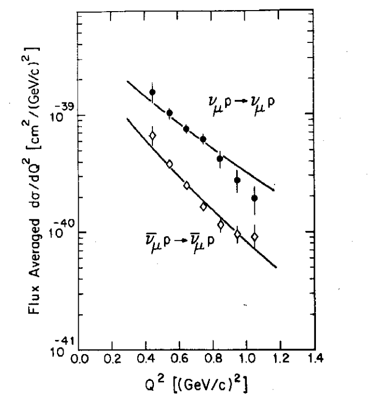
Figure 9: The data points are the measured flux–averaged differential cross sections for $\nu_{\mu}p\to\nu_{\mu}p$ and $\overline{\nu}_{\mu}p\to\overline{\nu}_{\mu}p$ measured in the experiment of Ref. [124]. The solid curves are best fits to the combined data with the values $M_{A}=1.06$ GeV and $\sin^{2}\theta_{W}=0.220$. The error bars represent statistical error and also include $Q^{2}$–dependent systematic errors. (Taken from Ref. [124])

The fit of the data presented in Ref. [124] was done under the assumption that the contribution of the strange form factors of the nucleon can be neglected and that the axial CC form factor is given by the dipole formula

$$G_{A}^{NC}(Q^{2})=\frac{1}{2}G_{A}(Q^{2})=\frac{1}{2}\frac{G_{A}(0)}{\displaystyle{\left(1+\frac{Q^{2}}{M_{A}^{2}}\right)^{2}}}$$ (9.28)

with $G_{A}(0)=1.26$. The parameters $M_{A}$ and $\sin^{2}\theta_{W}$ were considered as free parameters. From the simultaneous fit of the neutrino and antineutrino data the following values

$$\sin^{2}\theta_{W}=0.218^{+0.039}_{-0.047}$$

$$M_{A}=1.06\pm 0.05\,\mathrm{GeV}$$

were found (with $\chi^{2}=15.8$ at 14 DOF). The value of the axial cutoff $M_{A}$ was in a good agreement with the existing (at that time) world–average value

$$M_{A}=1.032\pm 0.036\,\mathrm{GeV}$$ (9.29)

which was found from the data of the experiments on quasi–elastic neutrino and antineutrino scattering. The solid curves in Fig. 9 were obtained with the above best–fit values of the parameters.

In Ref. [124] it was also reported the result of the fit of the data on NC elastic neutrino (antineutrino)–proton scattering under the assumption that the contribution of the strange vector form factors can be neglected and the axial strange form factor has the same $Q^{2}$ dependence as the CC axial form factor

$$G_{A}^{NC}(Q^{2})=\frac{1}{2}\frac{\left[G_{A}(0)-G_{A}^{s}(0)\right]}{\left(1+Q^{2}/M_{A}^{2}\right)^{2}}\,.$$ (9.30)

For the parameter $\sin^{2}\theta_{W}$ the value $0.22$ was taken. The parameter $M_{A}$ was constrained to the world–averaged value (9.29). From this fit it was found

$$G_{A}^{s}(0)=-0.12\pm 0.07\,.$$ (9.31)

Thus, from the results of the fit we described above, it follows that $-0.25\leq G_{A}^{s}(0)\leq 0$ at $90\%$ CL. It is necessary to stress, however, that there is a strong correlation between the values of the parameters $G_{A}^{s}(0)$ and $M_{A}$ (see Fig. 10)

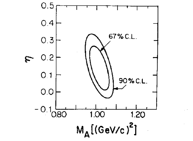
Figure 10: Simultaneous fit of $d\sigma/dQ^{2}$ for the neutrino and antineutrino elastic scattering samples in the ($M_{A},\eta$)–plane ($\eta\equiv-G_{A}^{s}(0)$), with $\sin^{2}\theta_{W}$ fixed at $0.220$. In the fit $M_{A}$ has been constrained at the world–average value $M_{A}=1.032\pm 0.036$ GeV. (Taken from Ref [124]).

The data of the BNL experiment were re–analyzed in Ref. [125]. In this work not only strange axial but also strange vector form factors, $F_{1}^{s}(Q^{2})$ and $F_{2}^{s}(Q^{2})$, were taken into account. It was assumed that all non–strange form factors have the same dipole $Q^{2}$–dependence, with $M_{V}=0.843$ GeV. The parameter $M_{A}$ was considered as a free parameter. It was also assumed that the electric form factor of the neutron is given by Eq. (8.26). These authors made several fits of the BNL data under different assumptions on the values of the parameters that characterize the strange form factors. For the latter the following parameterizations were chosen:

$$F_{2}^{s}(Q^{2}) =\frac{\mu_{s}}{(1+\tau)\left(\displaystyle{1+\frac{Q^{2}}{M_{V}^{2}}}\right)^{2}}\,,\qquad F_{1}^{s}(Q^{2})=\frac{F_{1}^{s}Q^{2}}{(1+\tau)\left(\displaystyle{1+\frac{Q^{2}}{M_{V}^{2}}}\right)^{2}}\,,$$

$$G_{A}^{s}(Q^{2}) =\frac{G_{A}^{s}(0)}{\left(\displaystyle{1+\frac{Q^{2}}{M_{A}^{2}}}\right)^{2}}\,,$$ (9.32)

which have the same (dominant) $Q^{2}$–dependence as the non–strange form factors. For the value of the parameter $\sin^{2}\theta_{W}$ the world average value $\sin^{2}\theta_{W}=0.2325$ was taken.

If we neglect the contribution of all strange form factors and keep as the only variable parameter $M_{A}$, then an acceptable fit to the data can be found with

$$M_{A}=1.086\pm 0.015\,{\mathrm{GeV}}$$

($\chi^{2}=14.12$ at 14 DOF). This value of $M_{A}$ is in a good agreement with the world–average value

$$M_{A}=1.061\pm 0.026\,{\mathrm{GeV}}\,.$$

If we neglect the contribution of the vector strange form factors only, the best fit to the data is obtained with:

$$G_{A}^{s}(0)=-0.15\pm 0.07;\qquad M_{A}=1.049\pm 0.019\,{\mathrm{GeV}}$$

($\chi^{2}=9.73$ at 13 DOF).

Hence there is a strong correlation between the values of parameters $M_{A}$ and $G_{A}^{s}(0)$. This correlation is connected with the fact that both negative values of $G_{A}^{s}(0)$ and larger values of $M_{A}$ increase the cross sections of neutrino– and antineutrino–proton scattering.

Finally, if we consider all strange form factors and $M_{A}$ to be variable parameters, then from the fit of the BNL data we get

$$\mu_{s} =-0.39\pm 0.70,\qquad F_{1}^{s} =0.49\pm 0.70\,{\mathrm{GeV}}^{-2}$$

$$G_{A}^{s}(0) =-0.13\pm 0.09,\qquad M_{A} =1.049\pm 0.023\,{\mathrm{GeV}}$$

($\chi^{2}=9.28$ at 11 DOF).

The authors of Ref. [125] concluded that from the data of the BNL experiment it is not possible to make firm conclusions on the values of the strange form factors of the nucleon. The result of the fit strongly depends on the value of the parameter $M_{A}$ which determines the $Q^{2}$ behavior of the axial CC form factor. Satisfactory fits were obtained for values of the strange axial form factor $G_{A}^{s}(0)$ in the range from 0 to $-0.15\pm 0.07$, depending on the value of $M_{A}$. There are no doubts that new experiments on the measurement of NC elastic neutrino (antineutrino) proton scattering are necessary.

Information on the strange axial constant of the nucleon $G_{A}^{s}(0)\equiv g_{A}^{s}$ can be obtained from the measurement of the ratio $R$ of the total cross sections for the production of protons and neutrons in quasi–elastic scattering of neutrinos (antineutrinos) on nuclei with isotopic spin equal to zero.

A detailed calculation was done for the nucleus ¹²C and for the neutrino beam of the Los Alamos Meson Physics Facility (LAMPF) (with neutrino energies less than 200 MeV) [126, 127]. The nuclear structure effects were taken into account in the framework of the random phase approximation; the final state interaction of the ejected nucleon was included through a finite–range force derived from the Bonn potential. Although this issue goes somewhat beyond the subject of this Section, we present it here since the original suggestion was founded on the hypothesis that nuclear structure and/or final state interaction effects appreciably cancel in the ratio of quasi–elastic $\nu(\overline{\nu})$–nucleus cross sections.

In order to illustrate the sensitivity of the method proposed in [126, 127], let us notice that the main contribution to the cross sections of quasi–elastic neutrino scattering comes from the axial NC form factor:

$$\sigma^{p,n}_{\nu}\propto\left|G_{A}^{NC}\right|^{2}\simeq\frac{1}{4}{G_{A}}^{2}\left(1\mp 2\frac{G_{A}^{s}}{G_{A}}\right)$$ (9.33)

For the ratio $R$ we have then:

$$R=\frac{\sigma^{p}_{\nu}}{\sigma^{n}_{\nu}}\simeq 1-4\frac{G_{A}^{s}}{G_{A}}\simeq 1-\frac{16}{5}G_{A}^{s}\,.$$ (9.34)

Thus, in the ratio of the cross sections the effect of the strange form factor is more than doubled. An important advantage of measuring the ratio $R$ is connected with the fact that this quantity is not affected by the absolute normalization of the cross sections.

A measurement of the above ratio is planned at the LSND detector at Los Alamos. The detector is made of mineral oil (CH₂) and reveals NC neutrino induced knockout reactions by measuring the energy deposition of the recoiling nucleons, with an energy resolution of 5% for nucleon kinetic energies $T_{N}>50$ MeV. The available neutrino beam is produced by pion in flight decay and is composed of about 80% neutrinos and 20% antineutrinos. The yields of protons and neutrons can be measured as a function of the recoiling nucleon kinetic energy, with an average over the nucleon angle, as the detector has no angular resolution. The total cross sections are then obtained by integrating the differential yields over the nucleon kinetic energy. While all neutron events come obviously from quasi–elastic scattering, the proton events can be produced both in free scattering on protons and in QE scattering on ¹²C, therefore a kinematical cut has to be applied in order to exclude free proton contributions, when forming the proton over neutron ratio. The maximum kinetic energy that can be transferred by the neutrinos available at Los Alamos to a free proton, at rest in the laboratory frame, is about 60 MeV; therefore the lower limit $T_{N}>60$ MeV is adopted in calculating the cross sections.

In Ref. [126] it was shown that in the range of neutrinos energies of LAMPF, the ratio $R$ practically does not depend on the neutrino energy and consequently on the uncertainties in the neutrino spectrum. In particular the ratio calculated averaging the cross sections over the expected neutrino spectrum was found to be practically the same as the one obtained for fixed $E_{\nu}=200$ MeV, a value which has been used in further studies (see Section 12).

It was also shown that the ratio of the cross sections for the scattering of neutrinos on free protons and neutrons differs from the ratio of the cross sections of the quasi–elastic knockout of protons and neutrons from ¹²C, calculated within the random phase approximation, by no more than $10\%$. This fact was presented as a reason for using the free expression as a qualitative guidance in understanding the role of the different contributions to the ratio. This small difference can also be taken as a first indication that the ratio $R$ weakly depends on nuclear effects. This argument will be further developed in Section 12.

Beside the axial form factor $G_{A}^{s}$ the effects of the strange form factor $F_{2}^{s}$ were also studied, while $F_{1}^{s}$ was not considered since its effects are expected to be small at the energies of interest for the Los Alamos experiment.

Since the Los Alamos beam is in fact a mixture of neutrinos and antineutrinos, the experimentally measured quantity will be obtained as the ratio of a “weighted average” of both types of cross sections, namely

$$\overline{R}_{LAMPF}=\frac{\langle\sigma_{\nu}^{p}\rangle+\langle\sigma_{\overline{\nu}}^{p}\rangle}{\langle\sigma_{\nu}^{n}\rangle+\langle\sigma_{\overline{\nu}}^{n}\rangle}$$ (9.35)

$\langle\sigma\rangle=\int\Phi(E)\,\sigma(E)\,dE$ being the cross section averaged over the neutrino or antineutrino flux $\Phi_{\nu(\overline{\nu})}(E)$.

The effects of $F_{2}^{s}$ are of opposite sign for neutrinos and antineutrinos, hence the sensitivity of the experimental ratio to $F_{2}^{s}$ can be reduced in the measured quantity (9.35). Due to the different rate of change of the separate $\nu$ and $\overline{\nu}$ cross sections with the strange axial form factor, the effects of $g_{A}^{s}$ on the experimental ratio can also be altered. In Ref. [127] it was found that assuming a spectrum made of 80% neutrinos and 20% antineutrinos the sensitivity of (9.35) to $g_{A}^{s}$ was increased with respect to the pure neutrino ratio, while the sensitivity to $F_{2}^{s}$ was decreased. The corresponding results are presented in Fig. 11, where the dependence of the ratio $\overline{R}$ on the axial strange constant $-G_{A}^{s}(0)$ is shown.

Notice, however, that a subsequent study [128], which used an updated spectrum for the antineutrinos, showed that the sensitivity of $\overline{R}$ to both $g_{A}^{s}$ and $F_{2}^{s}$ is close to the one of the pure neutrino ratio. An analysis of the experiment on the measurement of the ratio $R$ is going on at LAMPF [129]. It is planned that in this experiment the ratio $R$ should be measured with an accuracy of $10\%$. If $-G_{A}(0)<-0.2$ an effect of $G_{A}(0)$ will be seen.

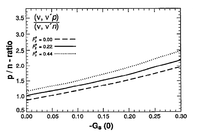
Figure 11: Ratio of the integrated proton– to neutron yield for the quasi–elastic neutrino induced reactions on ¹²C as a function of $-G_{A}^{s}(0)\equiv-G_{s}(0)$ in the conditions of the LAMPF decay–in–flight neutrino beam. The various curves correspond to different values of $F_{2}^{s}(0)\equiv\mu_{s}$. (Taken from Ref. [127])

10 Neutrino–antineutrino asymmetry in elastic neutrino (antineutrino)–nucleon scattering.

As we have seen before, the precise measurement of the cross sections of the NC neutrino (antineutrino) scattering on nucleons allows one to obtain direct information on the strange form factors of the nucleon if the electromagnetic form factors of proton and neutron and the CC axial form factor are known. At present there exist detailed information on the electromagnetic form factors of proton and neutron, which was obtained from the data of numerous experiments on elastic electron–proton and electron–deuteron scattering [130, 131]. New information on the electromagnetic form factors of the proton was recently obtained by the Jefferson Lab Hall A Collaboration [132], which measured the polarization of recoil protons in the scattering of polarized electrons on unpolarized protons. The axial form factor of the proton is rather poorly known and, as it was pointed out in the previous Section, the main problems in extracting information on the strange form factors from the existing neutrino (antineutrino)–proton data are connected with the uncertainty on the axial form factor.

In Ref. [133] a method was proposed, which allows one to obtain information on the strange form factors of the nucleon in a model independent way.

Let us consider the NC processes:

$$\nu_{\mu}+N \longrightarrow\nu_{\mu}+N$$ (10.1)

$$\overline{\nu}_{\mu}+N \longrightarrow\overline{\nu}_{\mu}+N\,.$$ (10.2)

The difference of the cross sections of the processes (10.1) and (10.2) are given by [see Eq. (9.9)]:

$$\left(\frac{d\sigma}{dQ^{2}}\right)^{NC}_{\nu}-\left(\frac{d\sigma}{dQ^{2}}\right)^{NC}_{\overline{\nu}}=\frac{2G_{F}^{2}}{\pi}y\left(1-\frac{1}{2}y\right)G_{M}^{NC}G_{A}^{NC}\,,$$ (10.3)

$y$ being defined as in Eq. (9.10). Hence, the above difference of the neutrino and antineutrino cross sections is determined only by the magnetic and axial NC form factors. The axial and magnetic NC form factors of the nucleon are given by Eqs. (4.22) and (4.24), respectively. The latter can be rewritten in the form:

$${G_{M}}^{NC;p(n)}=\pm G_{M}^{3}-2\sin^{2}\theta_{W}G_{M}^{p(n)}-\frac{1}{2}G_{M}^{s}$$ (10.4)

where $G_{M}^{3}=\frac{1}{2}(G_{M}^{p}-G_{M}^{n})$ is the isovector form factor of the nucleon.

Let us consider now the CC processes

$$\nu_{\mu}+n \longrightarrow\mu^{-}+p\,,$$ (10.5)

$$\overline{\nu}_{\mu}+p \longrightarrow\mu^{+}+n\,.$$ (10.6)

From Eq. (9.23) it follows that the difference of the cross sections of the reactions (10.5) and (10.6) is given by

$$\left(\frac{d\sigma}{dQ^{2}}\right)^{CC}_{\nu}-\left(\frac{d\sigma}{dQ^{2}}\right)^{CC}_{\overline{\nu}}=\frac{4G_{F}^{2}}{\pi}y\left(1-\frac{1}{2}y\right)G_{M}^{3}G_{A}\,.$$ (10.7)

Thus, this difference is determined by the isovector electromagnetic form factor and the CC axial form factor, which are the $u-d$ part of the magnetic and axial NC form factors of the nucleon.

Let us now define the following neutrino–antineutrino asymmetry:

$$\mathcal{A}(Q^{2})=\frac{\displaystyle{\left(\frac{d\sigma}{dQ^{2}}\right)^{NC}_{\nu}-\left(\frac{d\sigma}{dQ^{2}}\right)^{NC}_{\overline{\nu}}}}{\displaystyle{\left(\frac{d\sigma}{dQ^{2}}\right)^{CC}_{\nu}-\left(\frac{d\sigma}{dQ^{2}}\right)^{CC}_{\overline{\nu}}}}\,.$$ (10.8)

From Eqs. (10.3) and (10.7), we have

$$\mathcal{A}_{p(n)}=\frac{1}{4}\left(\pm 1-\frac{G_{A}^{s}}{G_{A}}\right)\left(\pm 1-2\sin^{2}\theta_{W}\frac{{G_{M}}^{p(n)}}{G_{M}^{3}}-\frac{1}{2}\frac{G_{M}^{s}}{G_{M}^{3}}\right)\,.$$ (10.9)

Thus, in the asymmetry $\mathcal{A}$ the strange axial and vector form factors enter in the form of the ratios ${G_{A}^{s}}/{G_{A}}$ and ${G_{M}^{s}}/{G_{M}^{3}}$. Taking into account only terms which depend linearly on the strange form factors we can rewrite Eq. (10.9) in the following form:

$$\mathcal{A}_{p(n)}=\mathcal{A}_{p(n)}^{0}\mp\frac{1}{8}\frac{G_{M}^{s}}{G_{M}^{3}}\mp\frac{G_{A}^{s}}{G_{A}}\mathcal{A}_{p(n)}^{0}$$ (10.10)

where

$$\mathcal{A}_{p(n)}^{0}=\frac{1}{4}\left(1\mp 2\sin^{2}\theta_{W}\frac{{G_{M}}^{p(n)}}{G_{M}^{3}}\right)$$ (10.11)

is the expected asymmetry in the case that all strange form factors are equal to zero. Thus, should it turn out that the measured asymmetry is different from $\mathcal{A}^{0}$, it would be a model independent proof that the strange form factors are not negligible with respect to the non–strange ones.

Usually in neutrino experiments nuclear targets are used. Accordingly we can average the asymmetry (10.8) over the protons and neutrons; then we obtain (assuming, e.g., an isospin symmetrical nucleus) the following expression:

$$\langle\mathcal{A}\rangle=\langle\mathcal{A}^{0}\rangle+\frac{1}{2}\sin^{2}\theta_{W}\frac{G_{M}^{0}}{G_{M}^{3}}\frac{G_{A}^{s}}{G_{A}}\,.$$ (10.12)

Here

$$\langle\mathcal{A}^{0}\rangle=\frac{1}{4}\left(1-2\sin^{2}\theta_{W}\right)$$

and ${G_{M}^{0}}=(G_{M}^{p}+G_{M}^{n})/2$ is the isoscalar magnetic form factor of the nucleon. In the expression for the averaged asymmetry $\langle\mathcal{A}\rangle$ only the axial strange form factor enters: in fact the interference between the (isoscalar) strange vector form factor and the isovector axial form factor vanishes after averaging over $p$ and $n$.

We notice that the electromagnetic form factors of the nucleon enter into the expression for the asymmetry $\mathcal{A}_{p(n)}(Q^{2})$ in the form of the ratio $G_{M}^{p(n)}/G_{M}^{3}$. It is well known that the electromagnetic form factors satisfy the approximate scaling relation

$$\frac{G_{M}^{p}(Q^{2})}{G_{M}^{n}(Q^{2})}=\frac{\mu_{p}}{\mu_{n}}$$ (10.13)

where $\mu_{p}$ and $\mu_{n}$ are the total magnetic moments of proton and neutron. Using the values

$$\mu_{p}=2.79,\qquad\mu_{n}=-1.91,\qquad\sin^{2}\theta_{W}=0.23,$$

we obtain the following expressions for the asymmetries in the scaling approximation

$$\mathcal{A}_{p} = 0.12-0.12\,\frac{G_{A}^{s}}{G_{A}}-0.13\,\frac{G_{M}^{s}}{G_{M}^{3}}$$

$$\mathcal{A}_{n} = 0.16+0.16\,\frac{G_{A}^{s}}{G_{A}}+0.13\,\frac{G_{M}^{s}}{G_{M}^{3}}$$

$$\langle\mathcal{A}\rangle = 0.14+0.02\,\frac{G_{A}^{s}}{G_{A}}\,.$$

Thus, the asymmetries $\mathcal{A}_{p}$ and $\mathcal{A}_{n}$ are rather sensitive to both axial and magnetic strange form factors. The contribution of the axial strange form factor to the averaged asymmetry $\langle\mathcal{A}\rangle$, instead, is suppressed due to the smallness of the isoscalar magnetic moment of the nucleon with respect to the isovector one.

The neutrino–antineutrino asymmetry depends on the ratio of the magnetic form factors of the proton and neutron. There exists a rather detailed information on the magnetic form factor of the proton in a wide range of $Q^{2}$ up to $30$ GeV² [134, 135, 136, 137, 138, 139]. The experimental data show that the behavior of the form factor at high $Q^{2}$ can not be described by the standard dipole formula.

The magnetic form factor of the neutron is less known than the one of the proton. A large part of the information on the neutron form factors has been obtained from experiments on the measurement of quasi–elastic scattering of electrons on deuterium and other nuclei [140, 141]. In order to extract from these data the electromagnetic form factors of the neutron it is necessary to take into account the neutron binding, final state interaction, contribution of meson exchange currents and other effects which rely on theoretical models.

In order to calculate the expected neutrino–antineutrino asymmetry with an error band connected with the uncertainties of the electromagnetic form factors, in Ref. [133] a fit of the data on the magnetic form factors of proton and neutron was done. The range $0.5~{}\mathrm{GeV}^{2}\leq Q^{2}\leq 10~{}\mathrm{GeV}^{2}$ was considered and the following two–poles formula was adopted for the magnetic form factor of the proton:

$$\frac{G_{M}^{p}}{\mu_{p}}=\frac{a_{1}}{1+a_{2}Q^{2}}+\frac{1-a_{1}}{1+a_{3}Q^{2}}\,.$$ (10.14)

It generalizes the dipole formula and was previously proposed in Ref. [142]. For the magnetic form factor of the neutron the expression

$$\frac{G_{M}^{n}}{\mu_{n}}=\frac{G_{M}^{p}}{\mu_{p}}\left(1+a_{4}Q^{2}\right)\,,$$ (10.15)

was taken, where the parameter $a_{4}$ takes into account the deviation from the scaling relation (10.13). From the fit of the data the following values for the parameters were found:

$$\begin{array}[]{l}a_{1}=-0.50\pm 0.04,\\ a_{2}=0.71\pm 0.02,\\ a_{3}=2.20\pm 0.04,\\ a_{4}=-0.019\pm 0.004\,.\end{array}$$ (10.16)

In the calculation of the expected asymmetry the parameterizations proposed in Ref. [130, 143] were also used.

The $Q^{2}$–behavior of the strange form factors is unknown. Different parameterizations of the strange form factors were thus considered in Ref. [133]. For the sake of illustration in Fig. 12 the result of the calculation of the asymmetry in the elastic neutrino (antineutrino)–proton scattering is shown.

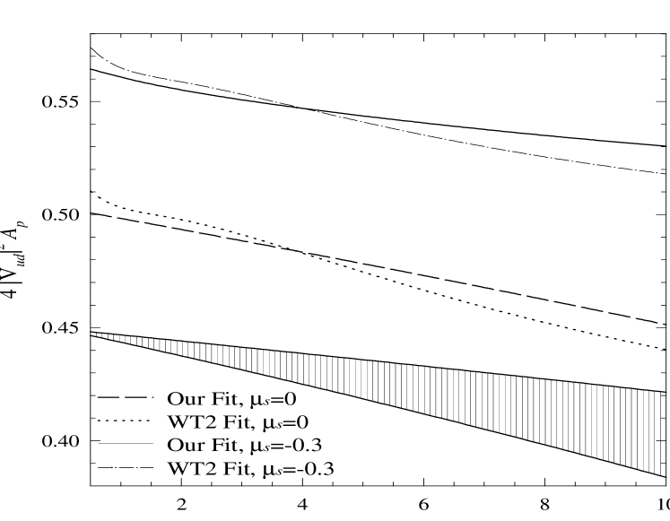
Figure 12: Plot of $4|V_{ud}|^{2}{\mathcal{A}}_{p}$ as a function of $Q^{2}$. The shadowed area corresponds to the uncertainty induced by the errors in the magnetic form factors in the absence of strange contributions. All the curves were obtained using a dipole form for $F_{A}^{s}(Q^{2})$ with $g_{A}^{s}=-0.15$. The dashed (dotted) curve was obtained with $G_{M}^{S}(Q^{2})=0$ utilizing the fit of Eqs. (10.14) and (10.15) (respectively, the WT2 fit [143]) for the magnetic form factors of the nucleon. The solid (dot–dashed) line was obtained using a dipole form for $G_{M}^{S}(Q^{2})$ with $\mu_{s}=-0.3$ and utilizing the fit of Eqs. (10.14) and (10.15) (respectively, the WT2 fit) for the magnetic form factors of the nucleon. (Taken from Ref. [133])

Here it was assumed that the strange form factors are given by the dipole formulas

$$G_{A}^{s}(Q^{2})=\frac{g_{A}^{s}}{\displaystyle{\left(1+\frac{Q^{2}}{{M_{A}^{s}}^{2}}\right)}}\,,\qquad G_{M}^{s}(Q^{2})=\frac{\mu_{s}}{\displaystyle{\left(1+\frac{Q^{2}}{{M_{V}^{s}}^{2}}\right)}}\,,$$ (10.17)

in which the following values were used for $M_{A}^{s}$ and $M_{V}^{s}$:

$$M_{A}^{s}=M_{A}=1.032~{}\mathrm{GeV},M_{V}^{s}=M_{V}=0.84~{}\mathrm{GeV}\,.$$ (10.18)

The dashed area was obtained under the assumption that $g_{A}^{s}=\mu_{s}=0$: it corresponds to the error band associated (to a confidence level of $90\%$) to the uncertainties (10.16) in the parameterization of the magnetic proton and neutron form factors . The dashed and dotted curves display the effect of the axial strange form factor (with $g_{A}^{s}=-0.15$) and correspond to different parameterizations ([133] and [143], respectively) of the electromagnetic form factors. These curves were obtained under the assumption that $\mu_{s}=0$. The solid and dot–dashed curves demonstrate the effect of both strange axial and vector form factors. They were obtained with $g_{A}^{s}=-0.15$ and $\mu_{s}=-0.3$. It is worth noticing that the slow variation of the asymmetry with $Q^{2}$ is due to the deviation of the magnetic form factors from the scaling relation (10.13).

Thus the measurement of neutrino–antineutrino asymmetry could allow one to resolve the contribution of the strange form factors. Let us notice that the combined effect of the axial and vector strange form factors depends on the relative sign of $g_{A}^{s}$ and $\mu_{s}$. If the sign are the same (as it is assumed in Fig. 12) the contribution of both form factors to the asymmetry sum up. Should the signs be opposite (which could be the case if $\mu_{s}>0$ [91]) the contributions to the asymmetry of the vector form factor would tend to compensate the effect of the axial one.

We have assumed in Eq. (10.17) that strange and non–strange form factors have the same $Q^{2}$ behavior. According to the asymptotic quark counting rule [144, 145], it would be natural to expect that the strange form factors decrease with $Q^{2}$ more rapidly than the non–strange ones. In this case the contribution of the strange form factors to the asymmetry will disappear at high $Q^{2}$. Calculations which consider this situation were made in Ref. [133] and show that the region $Q^{2}\simeq 1\div 2$ GeV is probably the optimal one to look for the effects of strangeness in neutrino–nucleon scattering.

11 The elastic scattering of neutrinos (antineutrinos) on nuclei with S=0 and T=0

In this Section we will consider the processes of the elastic NC scattering of neutrinos (antineutrinos) on nuclei with S=0 T=0 [104, 106, 146, 147].

$$\nu~{}(\overline{\nu})+A\longrightarrow\nu~{}(\overline{\nu})+A$$ (11.1)

The matrix element of the process for the scattering of neutrinos (antineutrinos) is given by the expression

$$\langle f|S|i\rangle=\mp\frac{G_{F}}{\sqrt{2}}\overline{u}(k^{\prime})\gamma^{\alpha}\left(1\mp\gamma_{5}\right)u(k)\langle p^{\prime}|J_{\alpha}^{NC}|p\rangle(2\pi)^{4}\delta^{(4)}(p^{\prime}-p-q)$$ (11.2)

Here $k$ and $k^{\prime}$ are the momenta of the initial and final neutrino (antineutrino), $q=k-k^{\prime}$, $p$ and $p^{\prime}$ are the momenta of the initial and final nucleus. The cross section of the processes (11.1) are given by the general expression (9.3).

The axial current, $A_{\alpha}^{NC}$, and the isovector part of the vector NC, $V_{\alpha}^{3}(1-2\sin^{2}\theta_{W})$, do not give contribution to the matrix element of the processes (11.1). For the isoscalar part of the vector NC we have, in general,

$$\langle p^{\prime}|V_{\alpha}^{NC}|p\rangle=n_{\alpha}F^{NC}(Q^{2})+q_{\alpha}G^{NC}(Q^{2})\,.$$ (11.3)

Here $n=p+p^{\prime}$, $q=p^{\prime}-p$ and $Q^{2}=2M_{A}T$ ($T$ is the kinetic energy of the final nucleus).

The form factor $G^{NC}(Q^{2})$ is equal to zero due to T–invariance of the strong interactions. The remaining form factor $F^{NC}(Q^{2})$ can be written in the form

$$F^{NC}(Q^{2})=-2\sin^{2}\theta_{W}F(Q^{2})-\frac{1}{2}F^{s}(Q^{2})$$ (11.4)

where $F(Q^{2})$ is the isoscalar electromagnetic form factor and $F^{s}(Q^{2})$ the strange form factor of the nucleus. From Eqs. (11.3) and (9.4) we have

$$W_{\alpha\beta}^{NC}=\frac{1}{4M^{2}}\,n_{\alpha}n_{\beta}\left[F^{NC}(Q^{2})\right]^{2}\delta\left(\nu-\frac{Q^{2}}{2M_{A}^{2}}\right)\,.$$ (11.5)

Then, from Eqs. (9.3) and (11.5) it follows that the cross sections of the scattering of neutrinos and antineutrinos on a nucleus with $S=0$, $T=0$ are equal to each other and are given by the expression

$$\frac{d\sigma_{\nu}}{dQ^{2}}=\frac{d\sigma_{\overline{\nu}}}{dQ^{2}}=\frac{G_{F}^{2}}{2\pi}\left(1-\frac{p\cdot q}{M_{A}E}-\frac{Q^{2}}{4E^{2}}\right)\left[F^{NC}(Q^{2})\right]^{2}$$ (11.6)

where $E$ is the neutrino energy in the laboratory system.

Thus, the strange form factor of the nucleus can be determined from the measurement of the cross section of the process (11.1) if the electromagnetic form factor of the nucleus $F(Q^{2})$ is known. The latter can be determined from the measurement of the cross section of the elastic scattering of unpolarized electrons on the nucleus, which is given by the expression

$$\frac{d\sigma_{e}}{dQ^{2}}=\frac{4\pi\alpha^{2}}{Q^{4}}\left(1-\frac{p\cdot q}{M_{A}E}-\frac{Q^{2}}{4E^{2}}\right)\left[F(Q^{2})\right]^{2}\,.$$ (11.7)

From Eqs. (11.6) and (11.7) we can find the relation connecting the strange form factor of the nucleus with the corresponding (measurable) cross sections:

$$F^{s}(Q^{2})=\pm 2F(Q^{2})\left\{\left(\frac{2\sqrt{2}\pi\alpha}{G_{F}Q^{2}}\right)\sqrt{\frac{(d\sigma_{\nu}/dQ^{2})}{(d\sigma_{e}/dQ^{2})}}\mp 2\sin^{2}\theta_{W}\right\}$$ (11.8)

or, equivalently, by extracting the elastic form factor from (11.7):

$$F^{s}(Q^{2})=\pm 2\frac{1}{{\sqrt{1-\frac{p\cdot q}{M_{A}E}-\frac{Q^{2}}{4E^{2}}}}}\left\{\sqrt{\frac{2\pi}{G_{F}^{2}}\frac{d\sigma_{\nu}}{dQ^{2}}}\mp 2\sin^{2}\theta_{W}\sqrt{\frac{Q^{4}}{4\pi\alpha^{2}}\frac{d\sigma_{e}}{dQ^{2}}}\right\}.$$ (11.9)

In Eqs. (11.8) and (11.9) the upper (lower) signs refer to a positive (negative) value of the quantity $4\sin^{2}\theta_{W}F+F^{s}$.

We remind the reader that the P–odd asymmetry in the scattering of polarized electrons on nuclei with $S=0$ and $T=0$ is determined by the ratio $F^{NC}/F$ [see Eq. (7.12)]. On the other hand the ratio of the cross sections (11.6) and (11.7) is determined by the ratio $(F^{NC}/F)^{2}$. Hence, by comparing (7.14) with (11.8), we find the following general relation between quantities, which are measurable in the scattering of neutrinos and electrons on nuclei with $S=0$ and $T=0$:

$$\mathcal{A}(Q^{2})=\pm\frac{\sqrt{(d\sigma_{\nu}/dQ^{2})}}{\sqrt{(d\sigma_{e}/dQ^{2})}}$$ (11.10)

where the plus (minus) sign have the same correspondence as in Eqs. (11.8) and (11.9).

Let us stress that the relation (11.10) takes place for any reactions of the type (7.1) and (11.1) in which the initial and final nuclei have $S=0$, $T=0$. It can be violated only if in the neutral current there are scalar and/or tensor terms.

The observation of the process of the scattering of neutrino on nuclei requires the measurement of the small recoil energy of the final nucleus. It could be easier to detect the process of scattering of neutrinos and electrons on nuclei if the nucleus undergoes a transition to excited states.

Let us consider, for example, the processes [106]

$$\nu+{{}^{4}}\mathrm{He} \longrightarrow\nu+{{}^{4}}\mathrm{He}^{*}$$

$$e+{{}^{4}}\mathrm{He} \longrightarrow e+{{}^{4}}\mathrm{He}^{*}$$

where ${{}^{4}}\mathrm{He}^{*}$ is the excited state of ${{}^{4}}\mathrm{He}$ with with $S=0$ and $T=0$ and excitation energy of $20.1$ MeV. This state can decay into $p$ and radioactive ³H [148]. The matrix element of the neutral current for the above processes is given by:

$$\langle p^{\prime}|J_{\alpha}^{NC}|p\rangle =\langle p^{\prime}|V_{\alpha}^{NC}|p\rangle=$$

$$=\left[2\left(p_{\alpha}-\frac{p\cdot q}{q^{2}}q_{\alpha}\right)F_{in}(Q^{2})+q_{\alpha}G_{in}(Q^{2})\right]\,.$$

It is obvious that the contribution of the form factor $G_{in}$ can be neglected. For the form factor $F_{in}$ we have

$$F_{in}^{NC}(Q^{2})=-2\sin^{2}\theta_{W}F_{in}(Q^{2})-\frac{1}{2}F_{in}^{s}(Q^{2})\,,$$ (11.12)

where $F_{in}(Q^{2})$ and $F_{in}^{s}(Q^{2})$ are the inelastic electromagnetic and strange form factors. All the relations that were obtained for the elastic case are valid also for the inelastic processes providing we change everywhere the elastic form factors by the inelastic ones and we use for $p\cdot q$ [e.g. in Eqs. (11.6) and (11.7)] the relation:

$$p\cdot q=\frac{1}{2}Q^{2}+\frac{1}{2}\left({M_{A}^{*}}^{2}-M_{A}^{2}\right)\,$$ (11.13)

$M_{A}^{*}$ being the mass of the excited state. Other $S=0,\,T=0$ nuclei, like ¹²C and ¹⁶O, could offer similar (perhaps better) possibilities of detecting $\nu$–induced transitions to $S=0,\,T=0$ excited states. Admittedly, the detection of the decay products of these excited states could be fairly difficult [149, 150]. Moreover, according to theoretical calculations [151], the strength of these isoscalar transitions is generally much weaker than the corresponding isovector ones. Yet, the measurement of the cross sections (11.6) and (11.7) (or the analogous ones for inelastic processes) would allow a model independent determination of the vector strange form factor of the nucleus.

12 Neutrino (antineutrino)–nucleus inelastic scattering

As we have seen in considering the Los Alamos future experiment and the BNL measurement of the axial strange form factor (see Section 9), one can consider neutrino scattering on both free nucleons and nucleons bound inside complex nuclei. The latter are convenient targets, as many neutrino detectors often contain nuclei as well as free protons. In fact even the Brookhaven “free” scattering data were mostly obtained from the scattering of $\nu,\overline{\nu}$ on Carbon, corrected for the Fermi motion and other nuclear effects.

In considering bound nucleons, especially at low energies such as the ones available at Los Alamos, it is important to be able to describe the effects of the nuclear many body structure and to evaluate the impact it can have on the measured quantities, in order to correctly interpret the experimental results in terms of single nucleon properties. Results from quasi–elastic (QE) electron scattering, which has been widely studied, can provide a guidance for selecting reliable nuclear models. However NC neutrino processes involve additional complications, with respect to the inclusive electron scattering. In fact, as the outgoing neutrino cannot be measured experimentally, an hadronic signature that the reaction has taken place has to be detected. The corresponding cross sections are therefore exclusive (or semi–inclusive) in the hadronic sector, similar to a coincidence electron scattering process, but inclusive in the leptonic sector, so that a detailed balance of the energy and momentum transfer is not possible any more.

In this Section we will summarize the studies which have been proposed in order to evaluate the impact of nuclear uncertainties on the extraction of the strange axial form factor of the nucleon from neutrino nucleus scattering, in particular from the measurement of the ratio which is under study at Los Alamos. A general review about neutrino–nucleus scattering processes can be found in [104].

We will consider the following processes,

$$\nu_{\mu}({\overline{\nu}_{\mu}})+A\longrightarrow\nu_{\mu}({\overline{\nu}_{\mu}})+N+(A-1)$$ (12.1)

in which a neutrino (antineutrino) of four–momentum $k$ interacts with a nucleus $A$ in its ground state and a nucleon is emitted, and detected, in the final state, with four–momentum $p_{N}=(E_{N},p_{N})$, while both the states of the daughter nucleus and the outgoing neutrino remain undetected.

Most of the models used in the literature describe the above quasi–free processes within the Impulse Approximation, where the neutrino is assumed to interact with only one nucleon, which is then emitted, the remaining nucleons being spectators. After the interaction with the neutrino, the struck nucleon can be considered as free (Plane Wave Impulse Approximation) or the residual interaction with the recoiling system can be taken into account, either directly or indirectly, through distorted wave functions. The different calculations proposed in the literature then differ by the models employed to describe the bound nucleus as well as the emitted nucleons. A schematic representation of the neutrino–nucleus scattering amplitude and, respectively, of its description within the PWIA is given in Figs. 13 and 14.

Figure 13: Schematic representation for the amplitude, in Born approximation, of the neutrino–nucleus scattering.

Figure 14: Representation of the $\nu$–nucleus scattering in the Plane Wave Impulse Approximation.

A model which has been employed very often in the literature is the Relativistic Fermi Gas (RFG), in which the bound and the outgoing nucleon are described by plane waves. Although the Fermi Gas is not completely realistic, thanks to its simplicity it is a useful guidance to understand the behavior of the different cross sections. Therefore, before illustrating various results, we briefly present the relevant formalism.

The RFG cross section is obtained by averaging over the nucleon momentum distribution the cross section for the scattering on a free moving nucleon of four–momentum $p$. Its general expression can thus be written as:

$$\left(\frac{d^{2}\sigma}{dE_{N}d\Omega_{N}}\right)_{\nu(\overline{\nu})} =\frac{G_{F}^{2}}{(2\pi)^{2}}\frac{3\mathcal{N}}{4\pi p_{F}^{3}}\frac{M^{2}|{\vec{p}}_{N}|}{k_{0}}\int\frac{d^{3}k^{\prime}}{k_{0}^{\prime}}\frac{d^{3}p}{p_{0}}\times$$

$$\times\delta^{(3)}\left({\vec{k}}-{\vec{k}}^{\prime}+{\vec{p}}-{\vec{p}}_{N}\right)\delta\left(k_{0}-k_{0}^{\prime}+p_{0}-E_{N}\right)\times$$

$$\times\theta(p_{F}-|{\vec{p}}\,|)\theta(|{\vec{p}}_{N}|-p_{F})\left(L^{\alpha\beta}\mp L_{5}^{\alpha\beta}\right)\left(W_{\alpha\beta}^{NC}\right)_{s.n.}\;,$$

where the integration over the momentum of the outgoing neutrino, $\vec{k}^{\prime}$, has been included explicitly. Here $(W_{\alpha\beta}^{NC})_{s.n.}$ is the single nucleon NC hadronic tensor, which is given by the following expression:

$$\left(W_{\alpha\beta}^{NC}\right)_{s.n.} =-\left[\tau\left(G_{M}^{NC}\right)^{2}+(1+\tau)\left(G_{A}^{NC}\right)^{2}\right]\left(g_{\alpha\beta}-\frac{q_{\alpha}q_{\beta}}{q^{2}}\right)+$$ (12.3)

$$+\left[\frac{\left(G_{E}^{NC}\right)^{2}+\tau\left(G_{M}^{NC}\right)^{2}}{1+\tau}+\left(G_{A}^{NC}\right)^{2}\right]\frac{X_{\alpha}X_{\beta}}{M^{2}}+$$

$$-\left(G_{A}^{NC}\right)^{2}\frac{q_{\alpha}q_{\beta}}{q^{2}}+\frac{i}{M^{2}}\epsilon_{\alpha\beta\mu\nu}p^{\mu}q^{\nu}G_{A}^{NC}G_{M}^{NC}$$

with

$$X_{\alpha}=p_{\alpha}-\frac{\left(p\cdot q\right)q_{\alpha}}{q^{2}}\,.$$

In Eq. (12) $L^{\alpha\beta}$ and $L_{5}^{\alpha\beta}$ are the leptonic tensor and pseudotensor, given in Eqs. (5.10) and (5.11), respectively; $p_{F}$ is the Fermi momentum of the nucleus under consideration, $(3\mathcal{N})/(4\pi p_{F}^{3})\theta(p_{F}-|\vec{p}\,|)$ is the momentum distribution of the nucleons in the RFG, ${\mathcal{N}=Z,N}$ being the number of protons or neutrons. We notice that the NC form factors which are contained in the hadronic tensor $\left(W_{\alpha\beta}^{NC}\right)_{s.n.}$ are different for protons and neutrons: hence the proton form factors have to be used in Eq. (12.3) when the QE emission of a proton is considered and, conversely, the neutron form factors have to be used when the emitted particle is a neutron. The function $\theta(|\vec{p}_{N}|-p_{F})$ takes into account the effects of Pauli Blocking on the ejected nucleon. The effects of an average binding energy of the bound nucleons can be taken into account by subtracting a (constant) term to the initial nucleon energy in the argument of the energy conserving delta function, $p_{0}\rightarrow p_{0}-B$.

Writing explicitly the contraction between the leptonic and the hadronic tensors the cross section becomes:

$$\left(\frac{d^{2}\sigma}{dE_{N}d\Omega_{N}}\right)_{\nu(\overline{\nu})} = \frac{G_{F}^{2}}{(2\pi)^{2}}\frac{3\mathcal{N}}{4\pi p_{F}^{3}}\frac{|{\vec{p}}_{N}|}{k_{0}}\int\frac{d^{3}k^{\prime}}{k_{0}^{\prime}}\frac{d^{3}p}{p_{0}}\delta\left(k_{0}-k_{0}^{\prime}+p_{0}-E_{N}\right)$$ (12.4)

$$\times \delta^{(3)}\left({\vec{k}}-{\vec{k}}^{\prime}+{\vec{p}}-{\vec{p}}_{N}\right)\theta(p_{F}-|{\vec{p}}\,|)\theta(|{\vec{p}}_{N}|-p_{F})$$

$$\times \left\{V_{M}(G_{M}^{NC})^{2}+V_{EM}\frac{(G_{E}^{NC})^{2}+\tau(G_{M}^{NC})^{2}}{1+\tau}+\right.$$

$$+ \left.V_{A}(G_{A}^{NC})^{2}\pm V_{AM}G_{A}^{NC}G_{M}^{NC}\right\}$$

where the form factors have been grouped as in Eq. (9.9) and

$$\begin{array}[]{l}V_{M}=2M^{2}\tau\left(k\cdot k^{\prime}\right)\\ V_{EM}=2\left(k\cdot p\right)\left(k^{\prime}\cdot p\right)-M^{2}\left(k\cdot k^{\prime}\right)\\ V_{A}=M^{2}\left(k\cdot k^{\prime}\right)+2M^{2}\tau\left(k\cdot k^{\prime}\right)+2\left(k\cdot p\right)\left(k^{\prime}\cdot p\right)\\ V_{AM}=2\left(k\cdot k^{\prime}\right)\left(k\cdot p+k^{\prime}\cdot p\right)\end{array}$$ (12.5)

The interesting quantities, related to the determination of the strange form factors of the nucleon, are then the single differential cross section

$$\left(\frac{d\sigma}{dT_{N}}\right)_{\nu(\overline{\nu})N}\equiv\left(\frac{d\sigma}{dE_{N}}\right)_{\nu(\overline{\nu})N}=\int\,d\Omega_{N}\left(\frac{d^{2}\sigma}{dE_{N}d\Omega_{N}}\right)_{\nu(\overline{\nu})N}\;,$$ (12.6)

where $T_{N}$ is the outgoing nucleon kinetic energy, the total (integrated over the nucleon energy) cross section

$$\sigma_{\nu(\overline{\nu})N}=\int\,dT_{N}\left(\frac{d\sigma}{dT_{N}}\right)_{\nu(\overline{\nu})N}$$ (12.7)

and the corresponding “proton over neutron” ratios

$${\mathcal{R}}_{\nu(\overline{\nu})} = \frac{\displaystyle{\left(\frac{d\sigma}{dT_{N}}\right)_{\nu(\overline{\nu})p}}}{\displaystyle{\left(\frac{d\sigma}{dT_{N}}\right)_{\nu(\overline{\nu})n}}},$$ (12.8)

$$R_{\nu(\overline{\nu})} = \frac{\sigma_{\nu(\overline{\nu})p}}{\sigma_{\nu(\overline{\nu})n}}\,.$$ (12.9)

An approximate expression for the RFG cross section can be obtained by inserting the explicit forms [Eqs. (4.22), (4.23), (4.24)] of the nucleonic NC form factors into Eq. (12.4) and neglecting both the terms proportional to $\left(1-4\sin^{2}(\theta_{W})\right)\simeq 0.075$ and the terms quadratic in the strange form factors. Under these approximations and using $\delta^{(3)}\left({\vec{k}}-{\vec{k}}^{\prime}+{\vec{p}}-{\vec{p}}_{N}\right)$ to integrate over ${\vec{k}}^{\prime}$ one obtains:

$$\left(\frac{d^{2}\sigma}{dE_{\scriptscriptstyle N}d\Omega_{\scriptscriptstyle N}}\right)^{NC}_{\scriptstyle{\left\{\begin{array}[]{l}\scriptstyle\nu p(n)\\ \scriptstyle{\overline{\nu}}p(n)\end{array}\right.}}=\frac{3Z(N)}{4\pi p_{F}^{3}}\frac{G_{F}^{2}}{(2\pi)^{2}}\frac{|{\vec{p}}_{\scriptscriptstyle N}|M^{4}}{k_{0}}\theta(|{\vec{p}}_{\scriptscriptstyle N}|-p_{F})\times$$ (12.12)

$$\qquad\times\int\frac{d^{3}p}{k^{\prime}_{0}p_{0}}\delta\left(k_{0}-k_{0}^{\prime}+p_{0}-E_{\scriptscriptstyle N}\right){\mathcal{I}}_{p(n)}(k,p,Q^{2})\,,$$ (12.13)

where (the plus/minus sign refer to the $\nu$ and ${\bar{\nu}}$ cases):

$${\mathcal{I}}_{p(n)}(k,p,Q^{2}) ={\mathcal{M}}_{p(n)}+2\tau^{2}G_{M}^{n(p)}G_{M}^{s}+$$ (12.14)

$$+\left[(z-\tau)^{2}-\tau(\tau+1)\right]\frac{G_{E}^{n(p)}G_{E}^{s}+\tau G_{M}^{n(p)}G_{M}^{s}}{1+\tau}+$$

$$-\delta_{p(n)}\left\{\left[(z-\tau)^{2}+2\tau(\tau+1)\right]G_{A}G_{A}^{s}\right.+$$

$$\left.\pm 2\tau(z-\tau)\left(G_{M}^{n(p)}G_{A}+G_{A}G_{M}^{s}-G_{M}^{n(p)}G_{A}^{s}\right)\right\},$$

with $\delta_{p}=1,\ \delta_{n}=-1$, $z=k\cdot p/M^{2}$ and, for scattering of massless leptons, $\tau=Q^{2}/4M^{2}=k\cdot k^{\prime}/2M^{2}=(k\cdot p-k\cdot p_{N})/2M^{2}$. The terms ${\mathcal{M}}_{p(n)}$ contain only the electromagnetic and axial form factors and are given by:

$${\mathcal{M}}_{p(n)} =\tau^{2}\left({G^{n(p)}_{M}}^{2}+G^{2}_{A}\right)+$$

$$+\frac{1}{2}\left[(z-\tau)^{2}-\tau(\tau+1)\right]\left[\frac{{G^{n(p)}_{E}}^{2}+\tau{G^{n(p)}_{M}}^{2}}{(1+\tau)}+G_{A}^{2}\right]\,.$$

The above equations, although approximate, can be useful to understand the interplay between strange and non–strange form factors in the cross sections (12.6), (12.7) and thus in the ratios (12.8), (12.9). We notice, however, that all the results presented in this Section were obtained without introducing any approximation.

The RFG was first applied to the study of neutrino–nucleon scattering in connection with the problem of nucleon strangeness by Horowitz et al. [152], and later employed by other authors [153, 154, 160]. The considered nucleus was ${}^{12}C$, for which the values $p_{F}=225$ $MeV$ and $B=25\div 27$ MeV are typically used.

A detailed analysis of the uncertainty induced by nuclear structure effects on the determination of axial strange form factor in $\nu$–nucleus QE scattering was proposed by Barbaro et al. in Ref. [153], both for the Los Alamos and the Brookhaven kinematical conditions.

In this paper the authors consider the processes (12.1) on ${}^{12}C$, using two different nuclear models: the RFG and an Hybrid Model (HM), in which the bound nucleons are described by harmonic oscillator shell model wave functions, while the outgoing nucleon is described by a plane wave. These choices are considered as two “extremes” among the available realistic nuclear models: in fact the RFG, using plane waves for the bound nucleons, can be seen as a “maximally unconfined” model, while the HM, whose bound single nucleon wave functions decrease more rapidly than the expected exponential behavior, is somehow “over-confined”. Moreover, while the RFG involves on-mass shell single nucleon amplitudes, the HM allows one to consider (half)-off shell nucleonic currents, thus providing an estimate of off-shellness effects. Therefore the difference between the effects of the strange form factors on the considered quantities calculated with these two models can provide an upper bound to the uncertainty induced by nuclear structure effects.

These two models were used to calculate both the differential and total cross sections [Eqs. (12.6) and (12.7)], for the neutrino–induced emission of a proton and of a neutron, for fixed neutrino energy. In this calculation the axial and axial strange form factors, $G_{A}$ and $G_{A}^{s}$, were assumed to have the same dipole $Q^{2}$–dependence, while strangeness contributions to the nucleonic vector current were not considered. It is important to notice that, contrary to what happens at the relatively high energies of BNL, under the Los Alamos kinematics the correlation between the value of the axial dipole cut-off mass and the strange axial constant $g_{A}^{s}$ is negligible, as shown in Refs. [82, 152], and thus at low energies the dipole parameterization can be used without introducing significant uncertainties .

The results of Ref. [153] for the kinematic conditions of Los Alamos ($E_{\nu}=200$ MeV) are shown in the upper and central panels of Figs. 15 and 16.

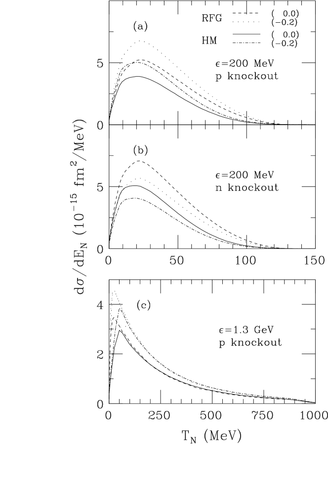
Figure 15: Differential cross sections $\left({d\sigma}/{dE_{N}}\right)_{\nu N}$, for the emission of a proton and of a neutron [panels (a) and (b), respectively] under the Los Alamos kinematic conditions, and for the emission of a proton for the average energy $E_{\nu}=1.3$ GeV of Brookhaven (panel c). The solid and dot-dashed lines correspond the the Hybrid Model mentioned in the text, without strangeness and with the strange axial constant set to $g_{A}^{s}=-0.2$, respectively. The dashed and dotted lines are obtained within the RFG, again with $g_{A}^{s}=0$ and $g_{A}^{s}=-0.2$, respectively. (Taken from Ref. [153])

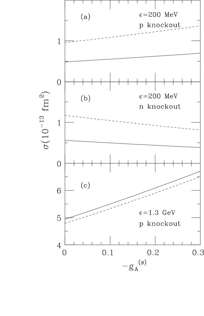
Figure 16: Total cross sections $\sigma_{\nu N}$ integrated over the nucleon kinetic energy ($T_{N}>60$ MeV for low energy neutrinos and $T_{N}>200$ MeV for higher energy neutrinos) as a function of the strange axial constant $-g_{A}^{s}$, for the emission of a proton (a) and of a neutron (b) at Los Alamos kinematics and for protons at Brookhaven kinematics (c). The solid lines correspond to the Hybrid Model described in the text, while the dashed lines are the RFG results. (Taken from Ref. [153])

From the comparison of their results on the separate cross sections at $E_{\nu}=200$ MeV, Barbaro and collaborators derive an uncertainty on $g_{A}^{s}$ due to nuclear model dependencies given by $\delta_{nucl}(g_{A}^{s})=\pm 0.25$, therefore larger than the expected value of $g_{A}^{s}$ itself. However, when the ratio of either differential or total cross sections is considered, this uncertainty is reduced by an order of magnitude, down to $\delta_{nucl}(g_{A}^{s})=\pm 0.015$. Including, in a worst case scenario, additional uncertainties due to off-shellness effects a final estimate $\delta_{nucl}(g_{A}^{s})=\pm 0.03$ is provided. This estimate is much smaller than the uncertainties on measurements of $g_{A}^{s}$ in deep inelastic scattering processes, and therefore these authors conclude that the proposed Los Alamos measurement is a very good way to determine $g_{A}^{s}$.

The same analysis was applied in [153] to the single cross section for the neutrino induced QE emission of a proton at $E_{\nu}=1.3$ GeV, the average energy of the BNL neutrino beam, as shown in the lower panels of Figs. 15 and 16. In this case nuclear structure effects are much smaller and the estimated uncertainty on the strange axial constant drops down to $\delta_{nucl}(g_{A}^{s})=\pm 0.015$. Both low and intermediate energy results are in agreement with the previous analysis proposed by Horowitz at al. [152] within the RFG, with and without binding energy effects.

The analysis of Barbaro et. al was carried on within the Plane Wave Impulse Approximation, thus not including the effects of Final State Interactions. The authors, however, concluded that the estimated value of $\delta_{nucl}(g_{A}^{s})$ for the p/n ratio can be considered as an upper bound also for the uncertainty associated with the use of more realistic nuclear models, which include FSI effects. Nonetheless, a detailed study of these effects has to be done, in order to be able to extract strangeness parameters from the proposed quantities.

As already mentioned in Section 9, FSI effects on the ratios (12.8) and (12.9) under the kinematical conditions typical of the Los Alamos facility were studied by Garvey et al. in Ref. [127], within the random phase approximation. In their calculations the ground state of Carbon was described as a Slater determinant of Woods-Saxon wave functions, the parameters of the WS potential being chosen in order to reproduce the ground state properties of ¹²C. FSI were included by means of a finite range G-matrix interaction, derived from the Bonn $NN$ potential. It was found that FSI can sizeably affect the separate cross sections, resulting in an increase of the latter of up to 40%, but these effects are mainly canceled in the ratio, where they amount to less than 10% and do not interfere with the effects of $g_{A}^{s}$. Similar results were obtained in a later calculation by Alberico et al. [154], who evaluated the ratio of differential cross sections, Eq. (12.8), within both the RFG and a Relativistic Shell Model. The latter included also FSI effects through a Relativistic Optical Potential. Again, FSI effects were found to be large on the separate cross sections, resulting in a decrease of the latter of up to 40%, mainly due to the absorption into different channels described by the imaginary part of the optical potential. However these effects on the p/n ratio were reduced to less than 10% and were found to be due mainly to the Coulomb repulsion, which is present for the protons only. In Ref. [154] FSI effects on the p/n ratio at Los Alamos kinematics were shown to be comparable with the effects of the magnetic strange form factor $G_{M}^{s}$. It is worth noticing that in Ref. [154] it was found that Final State Interactions can still be relevant, for the separate cross sections, even at relatively high energies ($E_{\nu}\simeq 1$ GeV).

Here we want to make a comment about a possible source of confusion: the authors [126, 127] who originally proposed the measurement of the ratio $R$ use the following definition for the nucleon kinetic energy, $T_{N}=T_{p}=T_{n}+2.77$ MeV, $2.77$ MeV being the average Coulomb repulsion for the protons. For the total cross sections (12.7) this translates into a different value for the lower limit of integration, namely $T_{p}^{min}=60$ MeV, $T_{n}^{min}=57.23$ MeV. Other authors [128, 153, 154], instead, use the same values $T_{N}=T_{p}=T_{n}$. While the choice of either definition does not affect the general considerations on both the sensitivity to the strange form factors and to the nuclear model effects, it was noticed in [128] that, when the experimental ratio given in Eq. (9.35) is considered, its numerical value can sensibly depend on the choice adopted. This has to be remembered when one is comparing results from different authors and especially when examining the future experimental data.

All calculations of the Los Alamos ratio so far considered were performed in the framework of the Impulse Approximation. Going beyond IA, Umino et al. [155, 156] evaluated the effects of two–body relativistic meson exchange currents (MEC) in neutrino–nucleus scattering at low and intermediate energies, within a soft–pion dominance model. The exchange current effects on the single differential cross sections (12.6) were calculated for both neutrinos and antineutrinos, for a fixed incident energy of $200$ MeV and under various assumptions for the strange form factors $G_{A}^{s}$ and $F_{2}^{s}$. These effects are strongly dependent on the value of the Fermi momentum and can be relatively large for $p_{F}\geq 350$ MeV. As an example, with $p_{F}=300$ MeV the $(\nu,\nu^{\prime},p)$ cross sections are reduced by MEC effects by about 20% at the peak; these corrections however become much less important (as already discussed for FSI) in the ratio of cross sections, Eq. (12.8). For Carbon, by assuming $p_{F}=225$ MeV, MEC contributions were found to be small for neutrino scattering and somewhat larger for the antineutrino cross sections, resulting in a reduction of the latter of about 15%. Moreover these effects are mainly confined to low values of the outgoing nucleon kinetic energy, $T_{N}\leq 50$ MeV, which is excluded by the kinematical cuts applied in the proposed LAMPF experiment, in order to select quasi–elastic events. Correspondingly, MEC corrections to the proton over neutron ratio were found to be limited to a few percent for the neutrino case and about 10% for the antineutrino one.

The possibility to extract information on the nucleonic strange form factors from a measurement of the ratios in Eqs. (12.8), (12.9) at energies higher than the ones available at LAMPF has been studied in Ref. [160], for neutrino and antineutrino energies of 1 GeV. Separate neutrino and antineutrino ratios were considered, both for differential and integrated cross sections. It was found that while the separate cross sections can still be rather sensitive to FSI effects, the nuclear model dependence is very weak in the ratios. The sensitivity of the ratios to the strange axial, magnetic and electric form factors as well as to the axial cut-off $M_{A}$ was studied in detail. For the axial and magnetic strange form factors the dipole parameterizations in Eq. (10.17) were used, while the electric strange form factor was assumed to be:

$$G_{E}^{s}(Q^{2})=\frac{\rho_{s}\tau}{\displaystyle{\left(1+\frac{Q^{2}}{M_{V}^{2}}\right)^{2}}}\,.$$ (12.16)

It was found that for the neutrino ratio the dominant effect is still due to $g_{A}^{s}$ and that this effect can still be large enough to allow an extraction of $g_{A}^{s}$ from a possible experiment, although its interplay with the strange magnetic form factor $G_{M}^{s}$ has to be carefully considered. On the other hand the antineutrino ratio can be rather sensitive to the electric strange form factor, $G_{E}^{s}$. However, although important as preliminary indications, these results can depend on the specific kinematical cuts somehow arbitrarily used in the calculation, and further investigation would be needed in case of a future experiment.

An illustration of these results is given in Fig. 17, where the ratio (12.9) of integral cross sections, calculated in the Relativistic Fermi Gas, is plotted as a function of the parameter $\mu_{s}$ for different values of $g_{A}^{s}$ and $\rho_{s}$.

Figure 17: The ratios (12.9) of the integrated NC neutrino and antineutrino–nucleus cross sections (12.7), as a function of $\mu_{s}$, evaluated in the RFG. The incident energy is $E_{\nu(\bar{\nu})}=1$ GeV and the integration limits for the cross sections are $100\leq T_{p}\equiv T_{n}\leq 400$ MeV. The solid line corresponds to $g_{A}^{s}=\rho_{s}=0$, in the other three curves [both in (a) and in (b)] $g_{A}^{s}=-0.15$ and $\rho_{s}=0$ (dashed line), $-2$ (dot–dashed line) and $+2$ (dotted line). (Taken from Ref. [160])

Finally let us go back to the neutrino–antineutrino asymmetry, introduced in Section 10 for the case of free nucleons. A more realistic approach would require to use the QE NC processes (12.1) together with the CC processes

$$\nu_{\mu}({\overline{\nu}_{\mu}})+A\longrightarrow\mu^{-}({\mu^{+}})+p(n)+(A-1)\,,$$ (12.17)

for the denominator. Since, as already noticed, the momentum transfer $Q^{2}$ cannot be determined in QE NC processes, the following asymmetry should be considered

$${\mathcal{A}(T_{N})}=\frac{\displaystyle{\left(\frac{d\sigma}{dT_{N}}\right)_{\nu}^{\mathrm{NC}}-\left(\frac{d\sigma}{dT_{N}}\right)_{\overline{\nu}}^{\mathrm{NC}}}}{\displaystyle{\left(\frac{d\sigma}{dT_{N}}\right)_{\nu}^{\mathrm{CC}}-\left(\frac{d\sigma}{dT_{N}}\right)_{\overline{\nu}}^{\mathrm{CC}}}}\;,$$ (12.18)

$T_{N}$ being, as usual, the kinetic energy of the ejected nucleon (proton or neutron).

Here the CC cross sections $\left({\displaystyle\mathrm{d}\sigma/\displaystyle{\mathrm{d}}T_{N}}\right)_{\nu(\overline{\nu})}^{\mathrm{CC}}$ in the denominator have been considered in analogy to the NC cross sections of Eq. (12.6).

The effects of nuclear structure on this asymmetry were studied in Ref. [154], by comparing the results obtained within two nuclear models: the RFG and a Relativistic Shell Model (RSM). The Shell Model wave functions were obtained as mean field solutions of a Dirac Equation derived from a linear Lagrangian, which includes nucleons, scalar ($\sigma$), vector–isoscalar ($\omega$) and vector–isovector ($\rho$) mesons. This model had been previously used in the study of $(e,e^{\prime}N)$ reactions on different nuclei [161, 162, 163]. The effects of Final State Interactions were described within the Distorted Wave Impulse Approximation, using, for the outgoing nucleon wave functions, the solutions of a Dirac equation with a phenomenological Relativistic Optical Potential (ROP), which includes scalar, vector and (for protons) Coulomb components [164]. When one is dealing with the CC cross sections entering in the denominator of the asymmetry (12.18), another type of “final state interactions” has to be considered, namely the Coulomb distortion of the outgoing leptons. This is expected to be small but it has to be taken into account since it is enhanced in the $\nu$–$\overline{\nu}$ difference in the denominator of (12.18) and can become relevant if other effects such as FSI are canceled in the ratio. In Ref. [154] Coulomb distortion was taken into account within the “effective impulse approximation”, which prescribes to modify the outgoing lepton plane wave $e^{i{\vec{k}}^{\prime}\cdot{\vec{r}}}$ according to:

$$e^{i{\vec{k}}^{\prime}\cdot{\vec{r}}}\rightarrow\frac{|\vec{k}\,^{\prime}_{eff}|}{|\vec{k}^{\prime}|}e^{i{\vec{k}_{eff}}\cdot{\vec{r}}}\;\;,$$ (12.19)

where

$${\vec{k}}\,^{\prime}_{eff}={\vec{k}}\,^{\prime}\left(1\pm\frac{3}{2}\frac{Z\alpha}{R|{\vec{k}}^{\prime}|}\right).$$ (12.20)

Here the plus (minus) refers to the lepton (anti-lepton), $Z$ is the number of protons and $R\simeq 1.2A^{1/3}$ is the effective charge radius of the nucleus under investigation. The validity of this approximation has been studied in electron scattering processes [165].

The asymmetry (12.18) was calculated in Ref. [154] for three typical values of the neutrino energy, 200 and 500 MeV and 1 GeV, using dipole–like parameterizations for both strange and non–strange form factors and the Galster parameterization for the electric form factor of the neutron [see Eq. (8.26)]. It was found that at low energies (200 MeV) the impact of nuclear uncertainties is too large to allow an unambiguous determination of the strange form factors from a measurement of $\mathcal{A}$. However at larger energies (already 500 MeV and especially 1 GeV) these effects are strongly reduced.

Results for $E_{\nu}=1$ GeV are shown in Fig. 18, where the asymmetry ${\mathcal{A}}$, for the emission (in the NC processes) of a proton, is plotted as a function of $T_{N}$ for three different choices of the strange form factors, as indicated in the caption. Here the solid curves represent the Shell Model Calculations without FSI effects, while RFG results are not displayed, since they coincide with the RSM ones. The dot-dashed curve shows the effects of FSI as described by the Relativistic Optical Potential. The effect on $\mathcal{A}$ of both FSI and Coulomb distortion is illustrated by the dotted line, which shows that, except for the region of small $T_{N}$, this combined effect is still small enough when it is compared with the effects of strangeness.

Figure 18: The asymmetry $\mathcal{A}$ for an ejected proton, Eq. (12.18), versus $T_{N}=T_{p}=T_{n}$, at incident $\nu({\overline{\nu}})$ energy $E_{\nu}=1.0$ GeV. The solid lines correspond to the RSM calculation without Final State Interactions, the dot–dashed lines include FSI effects through the ROP, the dotted lines represent the RSM corrected by both the FSI and the Coulomb distortion of the outgoing muon. The three sets of curves correspond to different choices of strangeness parameters: $g_{A}^{s}=\mu_{s}=0$ (lower lines), $g_{A}^{s}=-0.15$, $\mu_{s}=0$ (intermediate lines) and $g_{A}^{s}=-0.15$, $\mu_{s}=-0.3$ (upper lines). (Taken from Ref. [154])

A comment is required about the divergent behavior of the asymmetry in Fig. 18 for large $T_{N}$: this is associated with the effect of the outgoing lepton (a muon in this case) mass, which brings the CC cross sections down to zero more rapidly than the NC ones.

The authors of Ref. [154] considered also an “integral asymmetry”, obtained as the ratio of NC and CC differences between the total cross sections (12.7):

$$\mathcal{A}^{I}=\frac{\sigma_{\nu}^{NC}-{\sigma}_{\overline{\nu}}^{NC}}{\sigma_{\nu}^{CC}-\sigma_{\overline{\nu}}^{CC}}\;.$$ (12.21)

The corresponding curves for the emission of a proton are shown in Fig. 19.

Figure 19: The integral asymmetry, Eq. (12.21), $\mathcal{A}^{I}$ for an ejected proton, versus $g_{A}^{s}$, at incident $\nu({\overline{\nu}})$ energy $E_{\nu}=1.0$ GeV. The lower limit for the integration is $T_{N}=100$ MeV. The solid lines correspond to the RSM calculation, the dashed lines to the RFG with average binding energy of $25$ MeV, the dot–dashed lines include FSI effects. The two sets of curves correspond to different choices of the magnetic strangeness parameter: $\mu_{s}=0$ (lower lines) and $\mu_{s}=-0.3$ (upper lines). (Taken from Ref. [154])

Since the specific sensitivity of the asymmetries in Eqs. (12.18), (12.21) to the parameters characterizing the strange form factors of the nucleon derives from the cancellation of various contributions in the difference between neutrino and antineutrino cross sections, a crucial point, in considering realistic measurements, is the role played by the different shapes of the available neutrino and antineutrino spectra. This issue was addressed in Ref. [166] for the Brookhaven kinematical conditions: the integrated cross sections (12.7) were considered both for QE scattering on ${}^{12}C$ and for elastic scattering on free nucleons. The integral asymmetry $\mathcal{A}^{I}$ (12.21), calculated for $E_{\nu}=E_{\overline{\nu}}=1$ GeV, was compared with the following “flux–averaged asymmetry”:

$$\langle{\mathcal{A}^{I}}\rangle=\frac{\langle\sigma\rangle_{\nu}^{NC}-\langle\sigma\rangle_{\overline{\nu}}^{NC}}{\langle\sigma\rangle_{\nu}^{CC}-\langle\sigma\rangle_{\overline{\nu}}^{CC}}\,.$$ (12.22)

where the quantities $\langle\sigma\rangle_{\nu(\overline{\nu})}$ are the total cross sections averaged over the BNL neutrino and antineutrino spectra [see Eq. (9.24)] and the limits for the integrations over the outgoing nucleon kinetic energy and over the neutrino energy correspond to the kinematics of the BNL–734 Experiment [124], considered in Section 9. It was found that the effects of the folding amount to less than 2%, due to the similarity of the BNL $\nu$ and $\overline{\nu}$ spectra. In Fig. 20 the integral asymmetry $\mathcal{A}^{I}$ is plotted as a function of the strange axial constant $-g_{A}^{s}$. The solid line represents the folded asymmetry (12.22) for scattering on free protons, which has to be compared with the unfolded elastic asymmetry shown by the empty–dots. The dashed and dotted lines show results for the QE emission of protons, within the RFG, with and without folding. The curves obtained (without folding) using the Relativistic Shell Model described previously in this Section are also shown, confirming that at these energies nuclear effects on the asymmetry are small.

Figure 20: The integral asymmetry ${\mathcal{A}}^{I}$ for an ejected proton versus $-g_{A}^{s}$. The magnetic and electric strange form factors have been set to zero, while dipole parameterizations (with the same value of the cut-off mass) have been assumed for the axial CC and the axial strange form factors. The solid line corresponds to the “flux–averaged” $\nu(\overline{\nu})$–proton elastic scattering asymmetry, the empty dots to elastic scattering without folding at $E_{\nu(\overline{\nu})}=1$ GeV. Results for the QE asymmetry on ¹²C are shown by the following curves: dashed line (RFG, with folding), dotted line (RFG, unfolded), dot–dashed line (RSM, unfolded) and three–dot–dashed line (RSM+ROP, unfolded); all unfolded curves are evaluated at $E_{\nu(\overline{\nu})}=1$ GeV. (Taken from Ref. [166])

In Ref. [166] an indirect “experimental value” of the folded asymmetry (12.22) for $\nu p$ elastic scattering was derived from the measured ratios of total elastic and quasi–elastic cross sections given in Eqs. (9.25)–(9.27):

$$\langle\mathcal{A}^{I}\rangle=\frac{\displaystyle{R^{BNL}_{\nu}\left(1-R^{BNL}\right)}}{\displaystyle{1-R^{BNL}R^{BNL}_{\nu}/R^{BNL}_{\overline{\nu}}}}=0.136\pm 0.008\,(\mathrm{stat})\,\pm 0.019\,(\mathrm{syst})\,.$$ (12.23)

The sensitivity of the ratios $R^{BNL}_{\nu}$, $R^{BNL}_{\overline{\nu}}$, $R^{BNL}$ and of the folded asymmetry $\langle\mathcal{A}^{I}\rangle$ to the strange form factors of the nucleon was then studied, by assuming the usual dipole parameterization for the strange and non–strange form factors. The results for neutrino and antineutrino proton scattering in the kinematical conditions of the BNL–734 experiment are shown in Fig. 21. The quantities $R^{BNL}_{\nu}$, $R^{BNL}_{\overline{\nu}}$, $R^{BNL}$ and $\langle\mathcal{A}^{I}\rangle$ are plotted as functions of the strange magnetic moment $\mu_{s}$ for different values of the axial strange constant $g_{A}^{s}$ and of $\rho_{s}$, while the axial cutoff mass is assumed to be $M_{A}=1.032$ GeV. The horizontal dotted lines represent the experimental values and the shaded areas are the corresponding error bands. The latter are rather large and comparable with the effects of strangeness and it is clear that more precise measurements are needed in order to extract information on the strange form factors. Nevertheless we can observe that relatively large negative values of $g_{A}^{s}$ seem to be excluded by the antineutrino ratio $R^{BNL}_{\overline{\nu}}$. The other ratios and the asymmetry are compatible with relatively large, negative values of $g_{A}^{s}$: in this case a negative value of $\mu_{s}$ seems to be favored, in agreement with the findings of Ref. [125] but in contradiction with the SAMPLE results. In Ref. [166] the sensitivity of the above quantities to the axial cutoff mass was also studied, in the range $M_{A}=1.032\pm 0.036$ GeV: in accord with previous analyses [124, 125] the ratios $R^{BNL}_{\nu}$, $R^{BNL}_{\overline{\nu}}$, $R^{BNL}$ were found to be rather sensitive to $M_{A}$, while (assuming the same $Q^{2}$ dependence for $G_{A}$ and $G_{A}^{s}$) the asymmetry turned out to be practically independent of this parameter. Noticing that, as shown in Fig.21, the asymmetry does not depend on the electric strange form factor $G_{E}^{s}$ we can conclude that a more precise measurement of this quantity could allow one to obtain more “clean” information on $G_{A}^{s}$ and $G_{M}^{s}$.

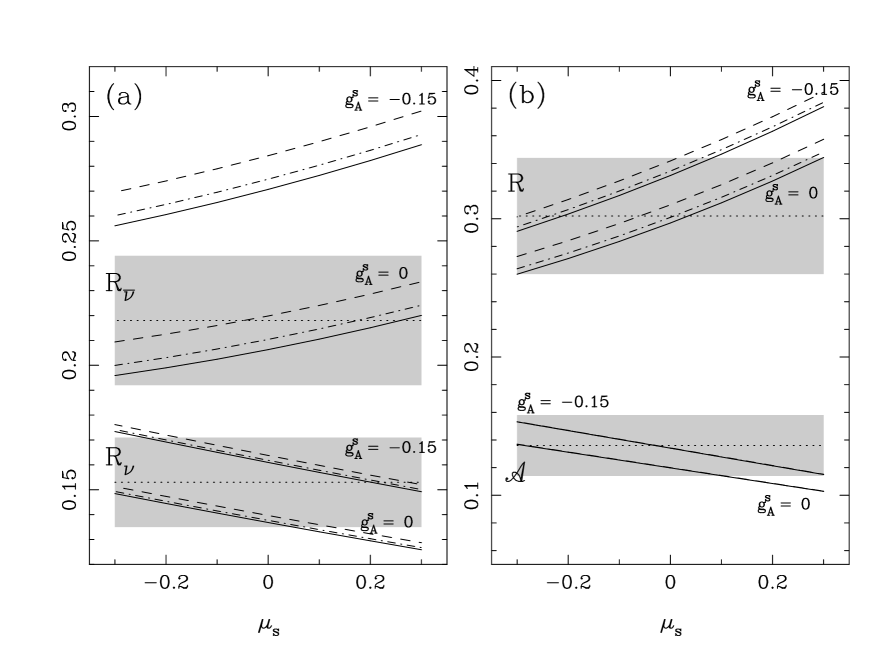
Figure 21: The ratios $R^{BNL}_{\nu}$, $R^{BNL}_{\overline{\nu}}$ and $R^{BNL}$, here indicated without the superscript $BNL$ and the folded asymmetry $\langle\mathcal{A}^{I}\rangle$ as functions of $\mu_{s}$. All curves correspond to $\nu(\overline{\nu})p$ elastic scattering in the kinematic conditions of Brookhaven. Results are shown for $g_{A}^{s}=0,\,-0.15$ and for $\rho_{s}=0$ (solid line), $\rho_{s}=-2$ (dot–dashed line) and $\rho_{s}=+2$ (dashed line). The shadowed regions correspond to the experimental data [Eqs. (9.25), (9.26), (9.27) and (12.23)] measured in the BNL–734 experiment. (Taken from Ref. [166])

Finally we notice that most of the studies of neutrino scattering QE processes we presented here consider the effects of negative values of $\mu_{s}$ only. This choice appeared to be favored by model calculations before the SAMPLE result relative to the proton data (see Section 6) was published. Instead, a positive $\mu_{s}$ would interfere with a negative $g_{A}^{s}$, reducing the effect of the latter, on both the p/n neutrino ratio and the $\nu-\overline{\nu}$ asymmetry, the size of this reduction being dependent on the actual value of $\mu_{s}$. However, as we have seen considering also the deuteron data, the SAMPLE result is still strongly affected by uncertainties due to radiative corrections and the error bands of the BNL–734 experiment do not allow to draw any definite conclusion. More stringent results have to be obtained before evaluating their quantitative impact on the neutrino cross sections and ratios.

13 Summary and Conclusions

The strange axial and vector form factors of the nucleon are an important issue which was under intensive experimental and theoretical investigations during the last decade. The first experimental evidence that the $Q^{2}=0$ value of the axial strange form factor of the nucleon, $g^{s}_{A}$, is unexpectedly large was obtained in 1989 in the famous EMC experiment (CERN) on the measurement of deep inelastic scattering of polarized muons on polarized protons. The EMC result triggered new DIS experiments at CERN, SLAC and DESY and hundreds of theoretical papers in which the connection of the constant $g^{s}_{A}$ with the strange quarks polarization and the polarization of gluons in the nucleon was elaborated in detail.

The EMC result also intensified the experimental and theoretical investigation of the problem of the strange form factors of the nucleon at relatively low values of $Q^{2}$ ($\leq 1$ GeV).

In order to obtain information on the strange form factors of the nucleon it is necessary to investigate Neutral Current induced processes. In the region of small $Q^{2}$ only the $u$, $d$ and $s$ parts of the NC should be taken into account. In the Standard Model there are three different components of the NC:

1. isovector (vector and axial) $u-d$ currents;

2. electromagnetic current;

3. strange (vector and axial) currents.

Thus, by using the available information on the electromagnetic and CC axial form factors of the nucleon, from the investigation of the NC induced lepton (electron and/or neutrino) nucleon processes we can obtain information on the strange axial and vector form factors of the nucleon.

This strategy can be realized by the investigation of:

• the P–odd asymmetry in the elastic scattering of polarized electrons on nucleons;

• neutrino(antineutrino) elastic scattering on nucleons;

In the case of electron–nucleon scattering in the region of small $Q^{2}$ the diagram with the exchange of a $\gamma$–quantum gives a much larger contribution to the matrix element of the process than the diagram with $Z^{0}$ exchange. Thus, the P-odd asymmetry, which arises from the interference between $\gamma$ and $Z^{0}$ exchanges, is very small ($\simeq 10^{-5}$ ). The measurement of such small asymmetries became possible only when very intense beams of highly polarized electrons and high resolution spectrometers were developed at MIT/Bates, Jefferson Lab and MAINZ . In Section 6 we have discussed the interesting results that were obtained in the latest experiments.

The P–odd asymmetry in the polarized electron–proton scattering is determined by the interference of the scalar electromagnetic and pseudoscalar $Z^{0}$–exchange parts of the amplitude, $aV^{NC}$ and $vA^{NC}$: the latter, however, occurs in the asymmetry multiplied by the small coefficient $g_{V}=-1/2+2\sin^{2}\theta_{W}$ (from the electron NC). Hence the P–odd asymmetry in $\vec{e}+p$ scattering is mainly sensitive to the strange vector form factors of the proton. On the other hand, the elastic and quasi–elastic scattering of polarized electrons on nuclei allows one to obtain complementary information: different choices of kinematics (e.g. backward versus forward scattering) and of nuclear targets can be used to select and eventually enhance the various hadronic NC components. At the moment this possibility has not been experimentally tested, but several experiments are under way or foreseen in the near future, which will measure the P-odd asymmetry in light nuclei (deuterium, ⁴He, etc.).

The NC neutrino (antineutrino) nucleon scattering allows one to obtain information both on the axial and vector strange form factors (see Section 9). Moreover, none of the contributions of the strange form factors to the cross sections of these processes is, in principle, suppressed. By investigating neutrino (antineutrino) nucleon scattering (as well as the P–odd asymmetry in electron–nucleon scattering) one can also hope to obtain information on the $Q^{2}$ behavior of the strange form factors. The most detailed investigation of neutrino (antineutrino) nucleon scattering was done in 1987 in the BNL–734 Brookhaven experiment, of which we discussed here in detail the results.

In order to obtain information on the strange form factors of the nucleon from the data of neutrino experiments it is necessary to know with good accuracy the $Q^{2}$ behavior of the CC axial form factor. There is no such information at present. Yet, we have discussed in Section 10 a method that allows one to obtain model independent information on the strange form factors of the nucleon. For this purpose it is necessary to measure the neutrino–antineutrino asymmetry. There is no doubt that with the many new neutrino experiments and the suggested new neutrino facility, the neutrino factory [167], the problem of the strange form factors of the nucleon will have new development.

It is worth mentioning that usually in neutrino experiments nuclear targets are used. A large part of this review is devoted to the detailed consideration of nuclear effects in the processes of neutrino (antineutrino) scattering on nuclei (see Sections 11 and 12). These effects are usually quite relevant on the single cross sections, but they can be drastically reduced when one considers ratios of cross sections. This fact has been widely underlined also in connection with the P–odd asymmetry in the (elastic or inelastic) scattering of polarized electrons on nuclei (see Sections 7 and 8).

Finally we mention that in the introductory parts (see Sections 1–4) many basic phenomenological relations are derived in sufficient detail, that they can easily be followed by the reader. We believe that this review will be useful for many physicists who are or will be interested in the problem of strangeness in the nucleon.

References

• [1] P. Vilain et al., CERN–EP/98–128 (1998).
• [2] S.A. Rabinowitz et al., Phys. Rev. Lett. 70 (1993) 134.
• [3] M. Abramowitz et al., Z. Phys. C 15 (1982) 19.
• [4] T. Adams et al. [NuTeV Collaboration], in: Bloomington 1999, Physics with a high luminosity polarized electron ion collider p. 337, hep–ex/9906038.
• [5] A.O. Bazarko et al., [CCFR Collaboration], Z. Phys. C 65 (1995) 189.
• [6] V. Barone, C. Pascaud and F. Zomer, Eur. Phys. J. C 12 (2000) 243.
• [7] M. Anselmino, A. Efremov and E. Leader, Phys. Rept. 261 (1995) 1.
• [8] B. Lampe and E. Reya, Phys. Rept. 332 (2000) 1.
• [9] B.W. Filippone and Xiangdong Ji, “The spin structure of the nucleon”, hep–ph/0101224
• [10] J. Ellis, “Strangeness and hadron structure”, hep–ph/0005322.
• [11] L.S. Brown, W.J. Pardee and R.D. Peccei, Phys. Rev. D 4 (1971) 2801.
• [12] T.P. Cheng and R.F. Dashen, Phys. Rev. Lett. 26 (1971) 594.
• [13] J. Gasser, M.E. Sainio and A. Svarc, Nucl. Phys. B 307 (1988) 779.
• [14] T.P. Cheng and L.F. Li, Gauge Theory of Elementary Particle Physics, Clarendon, Oxford, 1984.
• [15] J. Gasser, M. Leutwyler and M.E. Sainio, Phys. Lett. B 253 (1991) 252.
• [16] S. V. Wright, D. B. Leinweber and A. W. Thomas, Nucl. Phys. A 680 (2000) 137.
• [17] T.P. Cheng, Phys. Rev. D 38 (1988) 2896.
• [18] A. Bottino, F. Donato, N. Fornengo and S. Scopel, Astropart. Phys. 13 (2000) 215.
• [19] J. Ashman et al. [European Muon Collaboration], Nucl. Phys. B 328 (1989) 1.
• [20] B. Adeva et al. [Spin Muon Collaboration], Phys. Rev. D 58 (1998) 112002.
• [21] K. Abe et al. [E143 Collaboration], Phys. Rev. Lett. 74 (1995) 346.
• [22] K. Abe et al. [E143 Collaboration], Phys. Rev. Lett. 75 (1995) 25.
• [23] K. Abe et al. [E143 Collaboration], Phys. Rev. D 58 (1998) 12003.
• [24] P.L. Anthony et al. [E155 Collaboration], Phys. Lett. B 493 (2000) 19.
• [25] A. Airapetian et al. [HERMES Collaboration], Phys. Lett. B 442 (1998) 484.
• [26] K. Ackerstaff et al. [HERMES Collaboration], Phys. Lett. B 404 (1997) 383.
• [27] Hai–Yang Cheng, Chin. J. Phys. 38 (2000).
• [28] E.W. Hughes and R. Voss, Ann. Rev. Nucl. Part. Sci. 49 (1999) 303.
• [29] D.E. Groom et al. [Particle Data Group], Eur. Phys. J. C 15 (2000) 1.
• [30] G.M. Shore, “The proton spin crisis: Another ABJ anomaly?”, in Erice 1998, From the Planck length to the Hubble radius, p. 79, hep–ph/9812355.
• [31] C. H. Llewellyn Smith, hep-ph/9812301.
• [32] G. K. Mallot, in Proc. of the 19th Intl. Symp. on Photon and Lepton Interactions at High Energy LP99 ed. J.A. Jaros and M.E. Peskin, Int. J. Mod. Phys. A 15S1 (2000) 521.
• [33] K. Liu, J. Phys.G27 (2001) 511.
• [34] G. t’Hooft and M. Veltman, Nucl. Phys. B 44 (1972) 189.
• [35] R.D. Ball, S. Forte and G. Ridolfi, Phys. Lett. B 378 (1996) 255.
• [36] A. V. Efremov and O. V. Teryaev, “Spin Structure Of The Nucleon And Triangle Anomaly”, JINR-E2-88-287, Published in Czech. Hadron Symp. (1988) 302.
• [37] G. Altarelli and G.G. Ross, Phys. Lett B 212 (1988) 391.
• [38] see H.D. Politzer, Phys. Rept. 140 (1974) 129.
• [39] S. L. Glashow, Nucl. Phys. 22 (1961) 579.
• [40] S. Weinberg, Phys. Rev. Lett. 19 (1967) 1264.
• [41] A. Salam, in: Svartholm: Elementary Particle Theory, Proceedings Of The Nobel Symposium Held 1968 At Lerum, Sweden, Stockholm (1968) p. 367.
• [42] S. Weinberg, The quantum theory of fields, Vol. I and II (Cambridge Univ. Press, 1996).
• [43] M.E. Peskin and D.V. Schroeder, An introduction to Quantum Field Theory (Addison–Wesley Publ. Company, 1996).
• [44] C. Quigg, Gauge Theories of the Strong, Weak and Electromagnetic Interactions (Reading, Usa: Benjamin/Cummings, 1983) ( Frontiers In Physics, 56).
• [45] E. Leader and E. Predazzi, An Introduction to gauge theories and modern particle physics. (Cambridge, UK: Univ. Press, 1996) Vol.1
• [46] S.M. Bilenky, Introduction to Feynman Diagrams and Electroweak Interactions Physics, (Editions Frontieres, 1994).
• [47] C. Itzykson and J.B. Zuber, Quantum Field Theory (McGraw–Hill Book Co., 1988).
• [48] R.L. Jaffe, Phys. Lett. B 229 (1989) 275.
• [49] B.R. Holstein, in: Proceedings of the Caltech Workshop on Parity Violation in Electron Scattering, E.J. Beise and R.D. McKeown eds. (World Scientific, 1990) p. 27.
• [50] N.W. Park, J. Schechter and H. Weigel, Phys. Rev. D 43 (1991) 869.
• [51] N. W. Park and H. Weigel, Nucl. Phys. A 541 (1992) 453.
• [52] W. Koepf, E.M. Henley, and J.S. Pollock, Phys. Lett. B 288 (1992) 11.
• [53] S. Hong and B. Park, Nucl. Phys. A 561 (1993) 525.
• [54] T.D. Cohen, H. Forkel and M. Nielsen, Phys. Lett. B 316 (1993) 1.
• [55] S.C. Phatak and S. Sahu, Phys. Lett. B 321 (1994) 11.
• [56] M.J. Musolf and M. Burkardt, Z. Phys. C 61 (1994) 433.
• [57] W. Koepf and E.M. Henley, Phys. Rev. C 49 (1994) 2219.
• [58] H. Forkel et al., Phys. Rev. C 50 (1994) 3108.
• [59] H. Ito, Phys. Rev. C 52 (1995) R1750.
• [60] H. Weigel et al., Phys. Lett. B 353 (1995) 20.
• [61] H.W. Hammer, U. Meissner and D. Drechsel, Phys. Lett. B 367 (1996) 323.
• [62] D. Leinweber, Phys. Rev. D 53 (1996) 5115
• [63] H. Forkel, Prog. Part. Nucl. Phys. 36 (1996) 229.
• [64] Chr. V. Christov et al., Prog. Part. Nucl. Phys. 37 (1996) 91.
• [65] P. Geiger and N. Isgur, Phys. Rev. D 55 (1997) 299.
• [66] M.J. Ramsey–Musolf and H. Ito, Phys. Rev. C 55 (1997) 3066.
• [67] M.J. Musolf, H.W. Hammer and D. Drechsel, Phys. Rev. D 55 (1997) 2741.
• [68] W. Melnitchouk and M. Malheiro, Phys. Rev. C 55 (1997) 431.
• [69] S-T. Hong, B-Y. Park, and D-P. Min, Phys. Lett. B 414 (1997) 229.
• [70] U. Meissner, V. Mull, J. Speth, and J. W. Van Orden, Phys. Lett. B 408 (1997) 381.
• [71] B.-Q Ma, Phys. Lett. B 408 (1997) 387.
• [72] H.W. Hammer and M.J. Ramsey–Musolf, Phys. Lett. B 416 (1998) 5.
• [73] L.L. Barz et al., Nucl. Phys. A 640 (1998) 259.
• [74] S.J. Dong, K.F. Liu and A.G. Williams, Phys. Rev. D 58 (1998) 074504.
• [75] H.W. Hammer and M. J. Ramsey-Musolf, Phys. Rev. C 60 (1999) 045205.
• [76] T. Hemmert, B. Kubis and U. Meissner, Phys. Rev. C 60 (1999) 04550.
• [77] H. Forkel, F.S. Navarra and M. Nielsen, Phys. Rev. C 61 (2000) 055206.
• [78] D.B. Leinweber and A.W. Thomas, Phys. Rev. D 62 (2000) 074505.
• [79] L. Hannelius and D.O. Riska, Phys. Rev. C 62 (2000) 045204.
• [80] L. Hannelius, D.O. Riska and L.Y. Glozman, Nucl. Phys. A 665 (2000) 353.
• [81] S. Dubnicka, A. Z. Dubnickova and P. Weisenpacher, hep-ph/0102171.
• [82] M. J. Musolf, T. W. Donnelly, J. Dubach, S. J. Pollock, S. Kowalski and E. J. Beise, Phys. Rept. 239 (1994) 1.
• [83] see http://www.jlab.org/
and http://www.jlab.org/highlights/nuclear/Nuclear.html
• [84] K.A. Aniol et al. [HAPPEX Collaboration], nucl-ex/0006002, submitted to Phys. Rev. Lett..
• [85] M.J. Musolf and B.R. Holstein, Phys. Lett. B 242 (1990) 461.
• [86] S. Zhu, S. J. Puglia, B. R. Holstein and M. J. Ramsey-Musolf, Phys. Rev. D 62 (2000) 033008.
• [87] The numbers associated with the points in Fig. 2 correspond to the following reference numbers in the present work: [65]; [48]; [61]; [56]; [60]; [50]; [51]; [74]; [75]; [69]; [59]; [52]; [70]; [71].
• [88] H. Anklin et al., Phys. Lett. B 428 (1998) 248.
• [89] E.E.W. Bruins et al., Phys. Rev. Lett. 75 (1995) 21.
• [90] P.A. Souder, in: Bates 25 Symposium, Proceedings, Nov. 3–5, 1999, Cambridge, p. 291; JLab Experiment 99–115, K. Kumar and D. Lhuillier, spokespersons.
• [91] D.T. Spayde et al. [SAMPLE Collaboration], Phys. Rev. Lett. 84 (2000) 1106.
• [92] Ya.B. Zeldovich, Sov. Phys. JETP 12 (1961) 777.
• [93] C.S. Wood et al., Science 275 (1997) 759.
• [94] E.J. Beise, in: Bates 25 Symposium, Proceedings, Nov. 3–5, 1999, Cambridge, p. 305.
• [95] R. Hasty et al. [SAMPLE Collaboration], Science 290 (2000) 2117 [nucl-ex/0102001].
• [96] T. R. Hemmert, U. Meissner and S. Steininger, Phys. Lett. B 437 (1998) 184.
• [97] D. H. Beck and B. R. Holstein, hep-ph/0102053.
• [98] Opportunities for Nuclear Science at the MIT–Bates Accelerator Center, November 2000 (available at http://mitbates.mit.edu/news.stm).
• [99] MIT–Bates Experiment 00–04, T. Ito spokesperson.
• [100] F.E. Maas [A4 Collaboration], in: Parity Violation in Atoms and Polarized Electron Scattering, B. Frois and M.A. Bouchiai eds. (World Scientific Publ. Co., 1999) p. 491.
• [101] D.H. Beck, [G0 Collaboration], in: Parity Violation in Atoms and Polarized Electron Scattering, B. Frois and M.A. Bouchiai eds. (World Scientific Publ. Co., 1999) p. 502.
• [102] G. Feinberg, Phys. Rev. D 12 (1975) 3575.
• [103] J.D. Walecka, Nucl. Phys. A 285 (1977) 349.
• [104] T.W. Donnelly and R.D. Peccei, Phys. Rept. 50 (1979) 1.
• [105] D.H. Beck, Phys. Rev. D 39 (1989) 3248.
• [106] J. Bernabeu, S.M. Bilenky, J. Segura and S.K. Singh, Phys. Lett. B 282 (1992) 177.
• [107] CEBAF experiment 91–004, E.J. Beise spokesperson.
• [108] W. M. Alberico and A. Molinari, in: Parity Violation in Atoms and Polarized Electron Scattering, B. Frois and M.A. Bouchiai eds. (World Scientific Publ. Co., 1999), p. 389, nucl-th/9904026.
• [109] Jefferson Laboratory Experiment E–00–003, Spokespersons R. Michaels, P. A. Souder, G. M. Urciuoli.
• [110] C. J. Horowitz and J. Piekarewicz, astro-ph/0010227.
• [111] M. J. Musolf and T. W. Donnelly, Nucl. Phys. A546 (1992) 509.
• [112] W. Bertozzi, E. J. Moniz and R. W. Lourie, in: Frois, B. (ed.), Sick, I. (ed.): Modern topics in electron scattering (World Scientific, Singapore, 1991) 419.
• [113] M. J. Musolf and T. W. Donnelly, Z. Phys. C 57 (1993) 559.
• [114] T.W. Donnelly, M.J. Musolf, W.M. Alberico, M.B. Barbaro, A. De Pace and A. Molinari, Nucl. Phys. A 541 (1992) 525.
• [115] S. Galster, Nucl. Phys. B 32 (1971) 221.
• [116] S. Platchkov et al., Nucl. Phys. A 508 (1990) 343.
• [117] E. Hadjimichael, G.I Poulis and T.W. Donnelly, Phys. Rev. C 45 (1992) 2666.
• [118] L. Diaconescu, R. Schiavilla and U. van Kolck, nucl–th/0011034.
• [119] M. B. Barbaro, A. De Pace, T. W. Donnelly and A. Molinari, Nucl. Phys. A 569 (1994) 701.
• [120] M. B. Barbaro, A. De Pace, T. W. Donnelly and A. Molinari, Nucl. Phys. A 598 (1996) 503.
• [121] D.B. Kaplan and A. Manohar, Nucl. Phys. B 310 (1988) 527.
• [122] J. Ellis and M. Karliner, Phys. Lett. B 213 (1988) 73.
• [123] V. de Alfaro, S. Fubini, G. Furlan and C. Rossetti, Currents in hadron physics (North–Holland, Amsterdam, 1973).
• [124] L.A. Ahrens et al., Phys. Rev. D 35 (1987) 785.
• [125] G.T. Garvey, W.C. Louis and D.H. White, Phys. Rev. C 48 (1993) 761.
• [126] G.T. Garvey, S. Krewald, E. Kolbe and K. Langanke, Phys. Lett. B 289 (1992) 249.
• [127] G.T. Garvey, S. Krewald, E. Kolbe and K. Langanke, Phys. Rev. C 48 (1993) 1919.
• [128] E. Kolbe, S. Krewald and H. Weigel, Z. Phys. A 358 (1997) 445.
• [129] W.C. Louis, LSND Collaboration, LAMPF proposal 1173.
• [130] See P.E. Bosted, Phys. Rev. C 51 (1995) 509.
• [131] K. de Jager, in: Bates 25 Symposium, Proceedings, Nov. 3–5, 1999, Cambridge, p. 225 (hep–ex/0003034).
• [132] M.K. Jones et al. [Jefferson Lab Hall A Collaboration], Phys. Rev. Lett. 84 (2000) 1398.
• [133] W.M. Alberico, S.M. Bilenky, C. Giunti and C. Maieron, Z. Phys. C 70 (1996) 463.
• [134] L. Andivahis et al., Phys. Rev. D 50 (1994) 5491.
• [135] R.G. Arnold et al., Phys. Rev. Lett. 57 (1986) 174.
• [136] P.E. Bosted et al., Phys. Rev. C 42 (1990) 38.
• [137] P.N. Kirk et al., Phys. Rev. D 8 (1973) 63.
• [138] D. Krupa et al., J. Phys. G 10 (1984) 455.
• [139] W. Bartel et al., Nucl. Phys. B 58 (1973) 429.
• [140] A. Lung et al., Phys. Rev. Lett. 70 (1993) 718.
• [141] S. Rock et al., Phys. Rev. Lett. 49 (1982) 1139.
• [142] S.I. Bilen’kaya and Yu.M. Kazarinov, Sov. J. Nucl. Phys. 32 (1980) 382.
• [143] K. Watanabe and M. Takahashi, Phys. Rev. D 51 (1995) 1423.
• [144] S. J. Brodsky and B. T. Chertok, Phys. Rev. D 14 (1976) 3003.
• [145] S. J. Brodsky and J. F. Gunion, Phys. Rev. Lett. 37 (1976) 402.
• [146] T. Suzuki, T. Kohyama and K. Yazaki, Phys. Lett. B 252 (1990) 323.
• [147] E. M. Henley, G. Krein, S. J. Pollock and A. G. Williams, Phys. Lett. B 269 (1991) 31.
• [148] S. Fiarman and W.E. Meyerhoff, Nucl. Phys. A 206 (1973) 1.
• [149] F. Ajzenberg–Selove, Nucl. Phys. A 506 (1990) 1.
• [150] F. Ajzenberg–Selove, Nucl. Phys. A 460 (1986) 1.
• [151] J. Blomqvist and A. Molinari, Nucl. Phys. A 106 (1968) 545.
• [152] C.J. Horowitz, Hungchong Kim, D.P. Murdock and S. Pollock, Phys. Rev. C 48 (1993) 3078.
• [153] M.B. Barbaro, A. De Pace, T.W. Donnelly, A. Molinari and M.J. Musolf, Phys. Rev. C 54 (1996) 1954.
• [154] W.M. Alberico, M.B. Barbaro, S.M. Bilenky, J.A. Caballero, C. Giunti, C. Maieron, E. Moya de Guerra and J.M. Udías, Nucl. Phys. A 623 (1997) 471.
• [155] Y. Umino, J. M. Udías and P. J. Mulders, Phys. Rev. Lett. 74 (1995) 4993.
• [156] Y. Umino and J. M. Udías, Phys. Rev. C 52 (1995) 3399.
• [157] S. Schramm and C. J. Horowitz, Phys. Rev. C 49 (1994) 2777.
• [158] M. J. Musolf and T. W. Donnelly, Phys. Lett. B 318 (1993) 263.
• [159] M. J. Musolf, R. Schiavilla and T. W. Donnelly, Phys. Rev. C 50 (1994) 2173.
• [160] W.M. Alberico, M.B. Barbaro, S.M. Bilenky, J.A. Caballero, C. Giunti, C. Maieron, E. Moya de Guerra and J.M. Udías, Phys. Lett. B 438 (1998) 9.
• [161] J.M. Udías, P. Sarriguren, E. Moya de Guerra, E. Garrido, and J.A. Caballero, Phys. Rev. C 48 (1993) 2731.
• [162] J.M. Udías, P. Sarriguren, E. Moya de Guerra, E. Garrido, and J.A. Caballero, Phys. Rev. C 53 (1996) R1488.
• [163] J.M  Udías, Ph.D. Thesis, Universidad Autónoma de Madrid (1993).
• [164] for more details on the Relativistic Optical Potential used here see also S. Hama, B.C. Clark, E.D. Cooper, H.S. Sherif and R.L. Mercer, Phys. Rev. C 41 (1990) 2737; E.D. Cooper, S. Hama, B.C. Clark and R.L. Mercer, Phys. Rev. C 47 (1993) 297.
• [165] C. Giusti and F.D. Pacati, Nucl. Phys. A 473 (1987) 717.
• [166] W.M. Alberico, M.B. Barbaro, S.M. Bilenky, J.A. Caballero, C. Giunti, C. Maieron, E. Moya de Guerra and J.M. Udías, Nucl. Phys. A 651 (1999) 277.
• [167] see C. Albright et al., “Physics at a Neutrino Factory”, hep-ex/0008064.