BNL-HET-01/2 February 2001 hep-ph/0102266

Padé approximation to fixed order QCD calculations

Robert V. Harlander

HET, Physics Department
Brookhaven National Laboratory, Upton, NY 11973, U.S.A.
rharlan@bnl.gov

Padé approximations appear to be a powerful tool to extend the validity range of expansions around certain kinematical limits and to combine expansions of different limits to a single interpolating function. After a brief outline of the general method, we will review a number of recent applications and describe the modifications that have to be applied in each case. Among these applications are the $\overline{\mbox{\small MS}}$/on-shell conversion factor for quark masses and the top decay rate at NNLO in QCD.

Presented at the

5th International Symposium on Radiative Corrections
(RADCOR–2000)
Carmel CA, USA, 11–15 September, 2000

1 Introduction

The field of radiative corrections in quantum field theory has always been exciting and rapidly developing. At this conference various new methods were presented that allow us to keep up with the ever increasing complexity of the problems posed by modern particle physics. Some of these methods are concerned with the analytic evaluation of certain classes of Feynman diagrams (see, e.g., [1]). Equally important, however, is the development of systematic approximations for complex problems. As demonstrated in various physical applications, asymptotic expansions of Feynman diagrams prove to be a very efficient tool for this purpose: they provide recipes to reduce the number of dimensional scales (masses, momenta) that a diagram depends on (see, e.g., [2]). The result is a series (possibly asymptotic) in terms of ratios of these dimensional parameters.

However, the validity of an expansion is restricted to a certain – in general finite – region of convergence. As we will see, Padé approximations have been used to enlarge the validity range of these expansions. In some of the cases described below, expansions from different limits could be combined to construct an interpolating function which connects the individual, often non-overlapping regions of convergence.

The outline of this review is as follows: we will begin by describing the general method on the basis of the hadronic $R$ ratio. This quantity is extremely important in particle physics: not only is it directly measurable at $e^{+}e^{-}$ colliders, but it also influences other quantities, for example the running of the electro-magnetic coupling constant $\alpha_{\rm QED}(s)$ or the anomalous magnetic moment of the muon. The continuous efforts for an accurate evaluation of this quantity have presently reached an accuracy of order $\alpha_{s}^{3}$, even though only in the high energy limit. At order $\alpha_{s}^{2}$, due to the successful application of the Padé procedure described below, the full energy dependence is known. At first, the method was applied to non-singlet diagrams which clearly give the major contribution to $R$ (cf. Sect. 2). Sect. 3 will describe the generalizations that were necessary to evaluate the singlet contributions. Let us note that recently also non-diagonal currents have been taken into account. This opens a new field of applications related to charged current reactions, like single top production at hadron colliders.

The sections that follow are concerned with a different class of applications of the Padé procedure, namely the evaluation of on-shell quantities. First we describe a recent calculation of the conversion factor from the quark mass in the $\overline{\mbox{\small MS}}$ scheme to the on-shell scheme at order $\alpha_{s}^{3}$. Due to the progress in the field of heavy quark and top threshold physics, the evaluation of this factor was of utmost importance. The second application is the determination of NNLO QCD corrections to the top quark decay rate which is a necessary input for a precise experimental determination of the top quark properties at future colliders. Closely related is the evaluation of the muon decay rate at second order in QED, as well as $\Gamma(b\to ue\bar{\nu}_{e})$ to ${\cal O}(\alpha_{s}^{2})$. Each of the on-shell quantities above has been calculated by two independent groups with complementary methods. The agreement of the results once again confirms the validity and accuracy of the Padé method.

2 General procedure

We are not going to describe all the details of the procedure for constructing Padé approximants, because this has been done in the literature to a sufficient extent (see in particular [4, 5, 6, 7, 8, 9]). Nevertheless, for the sake of a closed presentation, let us give the main ideas by considering the by now “classic” example of the hadronic $R$ ratio:

$$\begin{split}R(s)={\sigma(e^{+}e^{-}\to\mbox{hadrons})\over\sigma(e^{+}e^{-}\to\mu^{+}\mu^{-})}\,.\end{split}$$ (1)

The leading two orders in $\alpha_{s}$ for $R(s)$ are known in analytic form. An analytic evaluation of the complete corrections at ${\cal O}(\alpha_{s}^{2})$ currently seems to be excluded. The exact answer is known only for certain contributions, in particular the terms involving a light fermion pair [10].

For the other contributions one has to rely on approximations. There are two obvious limiting cases for which this can be achieved: On the one hand, if the center-of-mass energy is very large, one may set the quark masses $m$ to zero. One may then use the equation

$$\begin{split}R(s)=12\pi\,{\rm Im}\Pi(s/(4m^{2})+i0_{+})\end{split}$$ (2)

which relates $R(s)$ to the imaginary part of the polarization function $\Pi(z)$ along the upper branch of the cut $z\in[1,\infty]$ in the complex plane. Sample diagrams for $\Pi(z)$ are shown in Fig. 1. For the moment we will restrict the discussion to diagrams where the external currents are connected by a single massive quark line (Fig. 1 (a) and (b)). Contributions where the external currents are connected by a massless quark line and where the massive quarks couple only to gluons (“gluon-splitting diagrams”) are numerically unimportant and shall not be addressed here. The modifications for diagrams where each of the external currents is connected to a separate Fermion line (“singlet diagrams”, Fig. 1 (c)) will be discussed in the next section.

Taking $m=0$ leads to massless propagator diagrams which can be calculated using the integration-by-parts algorithm [11] as implemented in the FORM program [12] MINCER [13]. One obtains

$$\begin{split}R(s)=3\bigg{\{}1+{\alpha_{s}\over\pi}+\left({\alpha_{s}\over\pi}\right)^{2}\left[{365\over 24}-11\zeta_{3}+n_{f}\left(-{11\over 12}+{2\over 3}\zeta_{3}\right)\right]\bigg{\}}+\ldots\,,\end{split}$$ (3)

where the ellipse indicates higher order terms in $\alpha_{s}$ and in $m^{2}/s$.

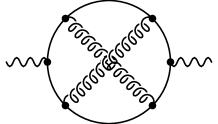
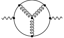
(a)	(b)	(c)

Figure 1: Diagrams contributing to the polarization function $\Pi(z)$. The solid lines are quarks, the springy ones are gluons. The wavy lines represent the external currents. (a) and (b) are non-singlet, (c) is a singlet diagram.

On the other hand, the leading behavior in the opposite limit, where the center-of-mass energy is close to threshold, i.e. $v\equiv\sqrt{1-4m^{2}/s}\ll 1$, can be deduced from the Sommerfeld-Sakharov formula and the two-loop result of the QCD potential (for details see [6, 7]). In general, these considerations allow one to deduce the terms that are singular for $v\to 0$ (cf. Coulomb singularity) as well as the constant term.

In both limits, however, one can do better. There are well-defined methods to obtain expansions around the exact limits $m=0$ and $s=4m^{2}$ (for reviews see [2, 14]). These methods reduce the original diagrams that depend on the two scales $m^{2}$ and $q^{2}$ to single-scale integrals which can be solved analytically. In this way one obtains approximations that are valid in certain ranges away from the actual limits. Fig. 2 shows the behavior of these expansions as dashed and dotted lines. It immediately becomes clear that their validity is restricted to a finite kinematical region. It is the purpose of this section to outline the procedure that leads to the solid lines in this figure, i.e. the construction of an approximation which is valid over the full $v$ range.

Figure 2: Threshold expansion up to terms of order $v\ln v$ [15] (dotted), high-energy expansion up to $m^{12}/s^{6}$ [16] (dashed), and Padé result [6] (solid). The singular and constant terms in $v$ have been subtracted and the renormalization scale is set to $\mu^{2}=m^{2}$. Left: $C_{\rm F}^{2}$-term; Right: $C_{\rm F}C_{\rm A}$-term ($C_{\rm F}=4/3$ and $C_{\rm A}=3$ are the Casimir operators of the fundamental and the adjoint representation of SU(3)).

The limits discussed above are the only two kinematically distinguished points for $R(s)$ at ${\cal O}(\alpha_{s}^{2})$ (we disregard the four-particle threshold at $s=16m^{2}$ here). Considering its connection to the polarization function $\Pi(z)$, however, (cf. Eq. (1)) there clearly is another interesting point, namely $z=0$. The coefficients of an expansion of $\Pi(z)$ around $z=0$ are called “moments”. Because of the cut at $z=1$, this expansion is expected to converge only for $|z|<1$, and at first it seems to be impossible to extract any information on $R(s)$ from it. However, one has to recall that $\Pi(z)$ is analytic everywhere in the complex plane, except along the cut. A mapping of the form

$$\begin{split}\omega={1-\sqrt{1-z}\over 1+\sqrt{1-z}}\end{split}$$ (4)

transforms the whole $z$-plane into the unit circle of the $\omega$-plane, such that the upper (lower) branch of the cut gets mapped to the upper (lower) semi-circle. The points at $|z|=\infty$ go to $\omega=-1$, while $z=0$ and $z=1$ correspond to $\omega=0$ and $\omega=1$, respectively.

In order to arrive at a smooth function that is easy to approximate, one subtracts the threshold singularities from $\Pi(z)$ (see above) as well as the logarithms of the asymptotic high-energy expansion (this has to be done in a suitable way in order not to generate logarithms for $z\to 0$). After some more manipulations one arrives at a function $P(\omega)$ whose value at $\omega=-1$ and whose first few Taylor coefficients around $\omega=0$ are in one-to-one correspondence to the expansion coefficients of $\Pi(z)$ around $z=0$ and $z=\infty$.

$P(\omega)$ is analytic within $|\omega|<1$ and thus its Taylor series around $\omega=0$ converges inside this region. However, we need the values of $\Pi(z)$ on the cut, or equivalently, $P(|\omega|=1)$. Thus one has to make sure that convergence of $P(\omega)$ is given not only for $|\omega|<1$, but also for $|\omega|=1$.

This is the point where Padé approximants come into play. The definition of an $[n/m]$-Padé approximant on a function $P(\omega)$ is

$$\begin{split}P_{[n/m]}(\omega)={a_{0}+a_{1}\omega+\cdots+a_{n}\omega^{n}\over 1+b_{1}\omega+\cdots+b_{m}\omega^{m}}\,.\end{split}$$ (5)

It has been demonstrated in [4, 5] that such an approximant extends the convergence region of the Taylor expansion to its border $|\omega|=1$. Performing the mapping back to the $z$-plane, and applying the inverse operations that led from $\Pi(z)$ to $P(\omega)$, we thus have constructed a function that approximates $\Pi(z)$ all over the complex plane, including the branches of the cut from $z=1$ to $z=\infty$. The imaginary part of this function gives rise to the solid lines in Fig. 2.

A nice feature of Padé approximation is that one has the freedom in varying the parameters $n$ and $m$ in Eq. (5). If convergence of the Padé approximants was not given, this would manifest itself in strong variations of the result for different values in $n$ and $m$. For $\Pi(z)$, for example, this dependence is so weak that different Padé approximants produce curves that would be hardly distinguishable from one another in Fig. 2 (see, e.g., [9]).

As it was mentioned above, this procedure was applied for the first time in [5] to the three-loop QED vacuum polarization. It was later on generalized to the QCD case [6] for various external currents [7] (vector, axial-vector, scalar, pseudo-scalar). In all of these papers, only the leading two terms in the asymptotic expansion around $z\to\infty$ were taken into account. After higher order terms in this limit became available [16], the method was extended to include them [8] and a further stabilization of the Padé predictions was observed [17, 9]. Recently [18] the method has been applied to non-diagonal currents in order to derive the dominant contributions to single top production at hadron colliders.

3 Padé approximation for singlet diagrams

Above we described in some sense the “optimal case”: information on both the limits $z\to 0$ and $z\to\infty$ was available, and the leading threshold behavior was known. Furthermore, the analytic structure of $\Pi(z)$ was such that the expansion around $z=0$ had the form of a plain Taylor expansion as opposed to an asymptotic series, i.e., it did not contain any logarithms of $z$. This is due to the fact that the discussion was restricted to the non-singlet contributions. The corresponding diagrams (cf. Fig. 1 (a) and (b)) do not have massless cuts: the external currents are connected by a single massive quark line, and cutting the diagram in halves always involves a cut through this line.

In the remaining part of this review we will be concerned with exceptions to this “optimal procedure.” The first case we will consider are the singlet contributions to $\Pi(z)$. They are distinguished from the non-singlet diagrams in the sense that the external currents are each connected to separate Fermion lines which in turn are connected to each other by gluons (cf. Fig. 1 (c)). If the external currents are vector-like, these diagrams vanish at ${\cal O}(\alpha_{s}^{2})$ due to Furry’s theorem. If, however, one is concerned with axial-vector, scalar, or pseudo-scalar currents, massless cuts occur.

These massless cuts spoil the analyticity of $P(\omega)$ (see Sect. 2) within $|\omega|<1$, and thus also the convergence of its expansion around $\omega=0$. Luckily, for the singlet diagrams the analytic expressions of the massless cuts are known. Thus, denoting these massless cuts as $R_{\rm ml}(s)$, we may employ the dispersion relation to write

$$\begin{split}&\Pi_{\rm S}(z)=\Pi_{\rm ml}(z)+\hat{\Pi}(z)\,,\quad\mbox{with}\quad\hat{\Pi}(z)=C^{-1}\int_{1}^{\infty}{\rm d}s{R_{\rm S}(s)\over s-4m^{2}z}\\ &\mbox{and}\quad\Pi_{\rm ml}(z)=C^{-1}\int_{0}^{1}{\rm d}s{R_{\rm S}(s)\over s-4m^{2}z}=C^{-1}\int_{0}^{1}{\rm d}s{R_{\rm ml}(s)\over s-4m^{2}z}\end{split}$$ (6)

($C=12\pi$ for external vector and axial-vector currents, $C=8\pi$ for scalar and pseudo-scalar currents). Here, $\Pi_{\rm S}(z)$ is the singlet contribution to the polarization function and

$$\begin{split}R_{\rm S}(s)=C\,{\rm Im}\Pi_{\rm S}(s/(4m^{2})+i0_{+})\,.\end{split}$$ (7)

$\hat{\Pi}(z)$ is analytic in the complex plane cut along $z\in[1,\infty]$. It can be obtained by evaluating $\Pi_{\rm ml}(z)$ through Eq. (6) and subtracting it from $\Pi_{\rm S}(z)$, i.e., the result for the singlet diagrams (see Fig. 1 (c)). One can then apply the Padé procedure outlined in Sect. 2 to $\hat{\Pi}(z)$.

For details on the evaluation of the integral for $\Pi_{\rm ml}(z)$ in Eq. (6) and the results we refer to [8]. At this point it shall be sufficient to mention that the combination of [7, 19] (non-singlet) and [8] (singlet) provides the current knowledge of $R(s)$ at ${\cal O}(\alpha_{s}^{2})$. Some contributions are known analytically, and the accuracy of the approximations in all the other cases is extremely good. Let us also remark that at ${\cal O}(\alpha_{s}^{3})$, $\Pi(z)$ is known in its high-energy expansion up to the terms $\propto m^{4}/s^{2}$ [20, 21, 22]. No moments for $z\to 0$ are available yet, and therefore a Padé approximation along the lines of the previous section is still out of reach.

As another application of the methods described above let us note that the results at ${\cal O}(\alpha_{s}^{2})$ were combined with the one-loop electro-weak corrections in order to predict the total cross section for $e^{+}e^{-}\to t\bar{t}$ at a linear collider [23].

4 Relation between $\overline{\rm MS}$ and on-shell quark mass

The $\overline{\mbox{\small MS}}$ scheme is a very convenient renormalization scheme, in particular from the technical point of view. Renormalization constants in the $\overline{\mbox{\small MS}}$ scheme do not depend on any masses or momenta, which means that their evaluation provides a certain freedom in choosing the particular set of diagrams to calculate. For example, the four-loop quark anomalous dimension was computed using two completely different approaches [24].

However, comparison of the theoretical results to experimental data often requires to express the involved quantities in terms of their on-shell values. This is why the conversion factor

$$\begin{split}z_{m}={M\over\bar{m}}\end{split}$$ (8)

that relates the on-shell to the $\overline{\mbox{\small MS}}$ quark mass is of great importance. In order to obtain this quantity, one has to evaluate the quark propagator

$$\begin{split}\Sigma(q)=q\!\!\!/\,\Sigma_{\rm V}(q^{2})+m\,\Sigma_{\rm S}(q^{2})\end{split}$$ (9)

at the on-shell point $q^{2}=m^{2}$, where $q$ is the external momentum and $m$ is the quark mass. A sample diagram that contributes to $\Sigma(q)$ at order $\alpha_{s}^{3}$ is shown in Fig. 3 (a).

(a)	(b)	(c)

Figure 3: Diagrams contributing to (a) $z_{m}$, (b) $\Gamma(t\to bW)$, and (c) $\Gamma(\mu\to e\bar{\nu}_{e}\nu_{\mu})$.

Technically, these diagrams carry only a single scale and should be accessible through the integration-by-parts algorithm [11]. However, it turns out that the level of complexity for $n$-loop on-shell diagrams is comparable to $(n+1)$-loop massive tadpole diagrams, for example. At the two-loop level, the problem of finding the recurrence relations was solved in [25].

The three-loop case seemed to be out of reach for quite some time. This is why the first calculation of the conversion factor was performed using a different, semi-analytic approach with the help of Padé approximants [26]. Looking at the Fermion propagator as a function of $z=q^{2}/m^{2}$ in the complex $z$ plane, we find a similar structure as for the polarization function $\Pi(z)$ in Sect. 2. $\Sigma_{\rm S,V}(q^{2})$ is analytic in the complex plane cut along $z\in[1,\infty]$. Thus, in principle one can follow the same strategy as for $\Pi(z)$: based on the expansions around $q^{2}=0$ and $q^{2}=\infty$ one constructs an approximation for $\Sigma_{\rm S,V}(q^{2})$ in the whole $q^{2}$ plane, including $q^{2}=m^{2}$ $(z=1)$, the point of interest.

A complication one has to face here is that the functions $\Sigma_{\rm S,V}(q^{2})$ depend on the strong gauge parameter $\xi$ in general. Only at the on-shell point $q^{2}=m^{2}$ are they gauge independent. Thus, the expansions around $z=0$ and $z=\infty$ explicitly contain $\xi$. If they could be re-summed exactly, $\xi$ would drop out in the limit $z\to 1$. But here the exact re-summation will be replaced by a Padé approximation and thus the result depends on $\xi$ even for $z=1$. However, the argumentation is that the dependence on $\xi$ is weak at $z=1$, in the sense that any “reasonable” choice of $\xi$ leads to valid predictions, with the spread among different choices being within the error of the Padé approximation. The question of what a “reasonable” choice is can be answered by making the natural assumption that a smooth curve gets better reproduced by Padé approximants than a strongly varying one. Looking at Fig. 4, it is not hard to decide that the favored values for $\xi$ are within a few units around $\xi=0$.

Figure 4: Gauge parameter dependence of $-g(z)$. ($g(z)$ is constructed from $\Sigma_{\rm S,V}(q^{2})$ in such a way that $g(1)=-z_{m}$ — for details see [26]). “F” denotes the ${\cal O}(\alpha_{s})$ contribution, “FF” the $C_{\rm F}^{2}$ term at ${\cal O}(\alpha_{s}^{2})$. The solid line corresponds to $\xi=-2$, the others to $\xi=-5,0,+2,+5$ (from short to long dashes) [Figures taken from [26]].

Following the outlined procedure, the authors of [26] were able to deduce the value of $z_{m}$ with an uncertainty of around $\pm 3\%$. Shortly after this result was presented, a second group published the analytical result for the conversion factor $z_{m}$ [27]. They managed to establish the recurrence relations for three-loop on-shell diagrams derived by integration-by-parts, which provides an extremely useful tool for various other applications (see also [28]).

5 Top decay to $\alpha_{s}^{2}$ and second order QED corrections to muon decay

The decay rate of the top quark is expected to be measured at future colliders with about 10% accuracy. This is roughly the size of the ${\cal O}(\alpha_{s})$ corrections to this quantity, which is why the evaluation of the $\alpha_{s}^{2}$ contribution was necessary. One option to evaluate this decay rate is to calculate the on-shell top quark propagator to the appropriate order and to take the imaginary part. A typical diagram whose imaginary part contributes to the rate $\Gamma(t\to bW)$ at order $\alpha_{s}^{2}$ is shown in Fig. 3 (b). In a first approximation, one may take the bottom quark and the $W$ boson to be massless. Then the lowest order diagram is a massless propagator. Starting from ${\cal O}(\alpha_{s})$, however, one is again faced with proper on-shell diagrams. In contrast to the problem of the $\overline{\mbox{\small MS}}$/on-shell conversion factor (see Sect. 4) the diagrams for $t\to bW$ contain massless cuts due to the presence of the $b$ and the $W$. The solution of [29] (see also [30]) to this problem was to evaluate the expansion around $q^{2}/m_{t}^{2}=0$ and to take the imaginary part before evaluating a Padé approximation. It is therefore not possible to take information from the limit $q^{2}\to\infty$ into account, because otherwise one receives contributions to the imaginary part coming from the cut starting at $q^{2}=m_{t}^{2}$.

Nevertheless, the Padé approximants constructed from the expansion around $q^{2}=0$ alone give a fairly accurate result (judging from the spread of the different approximants). In addition, it agrees well with an earlier result [31] which relied on an expansion around $1-m_{b}^{2}/m_{t}^{2}=0$. Considering the fact that these approaches are based on expansions around two completely different limits – which, in addition, are both far from the physical point – their agreement within very small error bars is a clear demonstration of the power of the applied methods.

Another example of this kind is the decay rate of the muon. Following a strategy closely related to the one described above for top decay, it was possible to evaluate the second order QED corrections to this quantity in a semi-analytical way [32]. Note, however, that the corresponding diagrams contain four closed loops here (cf. Fig. 3 (c)), even though one of them (made up by the neutrino lines) is always a massless self-energy insertion. Also in this case the Padé approximants agree nicely with the previously known analytical result [33] which provides an important check on the latter.

Along the same lines one can also obtain the corrections of order $\alpha_{s}^{2}$ to the decay rate $\Gamma(b\to ue\bar{\nu}_{e})$, the only technical difference being the presence of non-Abelian diagrams. Also here the semi-analytical result [32] approximates the analytical formula [34] to high accuracy.

6 Conclusions

We reviewed the method and recent applications of Padé approximation to fixed order calculations in QCD. Originally developed for the hadronic $e^{+}e^{-}$ cross section, the approach proved to be useful also for a completely different class of problems related to on-shell phenomena, for example in heavy quark physics. Let us conclude by pointing out that the continuously refining field of expansion techniques for Feynman diagrams (see [2]) should pave the way to numerous new applications for the Padé method.

Acknowledgments.

I would like to thank the organizers of the RADCOR-2000 symposium for the invitation, and all the participants for the pleasant and fruitful atmosphere during the conference. Travel support from the High Energy Group at BNL, DOE contract number DE-AC02-98CH10886, is acknowledged.

References

- [1] T. Gehrmann and E. Remiddi, these proceedings [hep-ph/0101147].
- [2] V.A. Smirnov, these proceedings [hep-ph/0101152].
-
[3]
M.A. Samuel, J. Ellis, and M. Karliner,
Phys. Rev. Lett. 74 (1995) 4380;
J. Ellis, M. Karliner, and M.A. Samuel, Phys. Lett. B 400 (1997) 176. -
[4]
D.J. Broadhurst,
J. Fleischer, and O.V. Tarasov, Z. Phys. C 60 (1993) 287;
J. Fleischer and O.V. Tarasov, Z. Phys. C 64 (1994) 413. - [5] P.A. Baikov and D.J. Broadhurst, Proc. of the 4th International Workshop on Software Engineering and Artificial Intelligence for High Energy and Nuclear Physics (AIHENP95), Pisa, Italy, 3-8 April 1995; [hep-ph/9504398].
- [6] K.G. Chetyrkin, J.H. Kühn, and M. Steinhauser, Phys. Lett. B 371 (1996) 93; Nucl. Phys. B 482 (1996) 213.
- [7] K.G. Chetyrkin, J.H. Kühn, and M. Steinhauser, Nucl. Phys. B 505 (1997) 40.
- [8] K.G. Chetyrkin, R. Harlander, and M. Steinhauser, Phys. Rev. D 58 (1998) 014012.
- [9] J.H. Kühn, Proc. of the 4th International Symposium on Radiative Corrections (RADCOR 98), Barcelona, Spain, 8-12 Sep 1998; [hep-ph/9901330].
-
[10]
A.H. Hoang, J.H. Kühn, and T. Teubner, Nucl. Phys. B 452 (1995) 173;
A.H. Hoang, M. Jeżabek, J.H. Kühn, and T. Teubner, Phys. Lett. B 338 (1994) 330. -
[11]
F.V. Tkachov, Phys. Lett. B 100 (1981) 65;
K.G. Chetyrkin and F.V. Tkachov, Nucl. Phys. B 192 (1981) 159. - [12] J.A.M. Vermaseren, [math-ph/0010025].
- [13] S.A. Larin, F.V. Tkachov,and J.A.M. Vermaseren, Rep. No. NIKHEF-H/91-18 (Amsterdam, 1991).
- [14] R. Harlander, Act. Phys. Pol. B 30 (1999) 3443.
- [15] A. Czarnecki and K. Melnikov, Phys. Rev. Lett. 80 (1998) 2531.
-
[16]
K.G. Chetyrkin, R. Harlander, J.H. Kühn, and
M. Steinhauser,
Nucl. Phys. B 503 (1997) 339;
R. Harlander and M. Steinhauser, Phys. Rev. D 56 (1997) 3980; Eur. Phys. J. C 2 (1998) 151. - [17] R. Harlander, PhD thesis, Karlsruhe University (Shaker Verlag, Aachen, 1998).
- [18] K.G. Chetyrkin and M. Steinhauser, [hep-ph/0012002].
- [19] A.H. Hoang, M. Jeżabek, J.H. Kühn, and T. Teubner, Phys. Lett. B 338 (1994) 330; A.H. Hoang, J.H. Kühn, and T. Teubner, Nucl. Phys. B 452 (1995) 173; A.H. Hoang and T. Teubner, Nucl. Phys. B 519 (1998) 285.
-
[20]
S.G. Gorishny, A.L. Kataev, and S.A. Larin,
Phys. Lett. B 259 (1991) 144;
L.R. Surguladze and M.A. Samuel, Phys. Rev. Lett. 66 (1991) 560; (E) ibid., 2416;
K.G. Chetyrkin, Phys. Lett. B 391 (1997) 402. - [21] K.G. Chetyrkin and J.H. Kühn, Phys. Lett. B 248 (1990) 359.
- [22] K.G. Chetyrkin, R.V. Harlander, and J.H. Kühn, Nucl. Phys. B 586 (2000) 56.
- [23] J. Kühn, T. Hahn, and R. Harlander, Proc. of the 4th International Workshop on Linear Colliders (LCWS 99), Sitges, Barcelona, Spain, 28 Apr-5 May 1999; [hep-ph/9912262].
-
[24]
K.G. Chetyrkin, Phys. Lett. B 404 (1997) 161;
J.A.M. Vermaseren, S.A. Larin, and T. van Ritbergen, Phys. Lett. B 405 (1997) 327. - [25] N. Gray, D.J. Broadhurst, W. Grafe, and K. Schilcher, Z. Phys. C 48 (1990) 673.
- [26] K.G. Chetyrkin and M. Steinhauser, Phys. Rev. Lett. 83 (1999) 4001; Nucl. Phys. B 573 (2000) 617.
- [27] K. Melnikov and T. van Ritbergen, Phys. Lett. B 482 (2000) 99.
- [28] A. Czarnecki, these proceedings.
- [29] K.G. Chetyrkin, R. Harlander, T. Seidensticker, M. Steinhauser, Phys. Rev. D 60 (1999) 114015.
- [30] A. Czarnecki and K. Melnikov, Proc. of the Lake Louise Winter Institute: Quantum Chromodynamics, Lake Louise, Alberta, Canada, 15-21 Feb 1998; [hep-ph/9806258].
- [31] A. Czarnecki and K. Melnikov, Nucl. Phys. B 544 (1999) 520.
- [32] T. Seidensticker and M. Steinhauser, Phys. Lett. B 467 (1999) 271.
- [33] T. van Ritbergen and R.G. Stuart, Phys. Rev. Lett. 82 (1999) 488.
- [34] T. van Ritbergen, Phys. Lett. B 454 (1999) 353.