May 2001

Vector and axial-vector correlators in a
chirally symmetric model
M. Urban, M. Buballa and J. Wambach

Institut für Kernphysik, TU Darmstadt, Schlossgartenstr. 9, 64289 Darmstadt, Germany

We present a chirally symmetric hadronic model for the vector and axial-vector correlators in vacuum. The dominant contributions to these correlators come from intermediate pions, $\rho$ and $a_{1}$ mesons which are calculated in one-loop approximation. The resulting spectral functions are compared with the data obtained by the ALEPH collaboration from $\tau$ decay. In the vector channel we find good agreement up to $q^{2}=1\;\mathrm{GeV}^{2}$, in the transverse axial-vector channel up to $q^{2}=2\;\mathrm{GeV}^{2}$, corresponding to the regimes dominated by two-pion or three-pion decay channels, respectively. The longitudinal axial correlator is in almost perfect agreement with the PCAC result.

1 Introduction

The investigation of matter under extreme conditions and the modifications of hadron properties with density or temperature is one of the main topics in intermediate and high-energy nuclear physics. Experimentally, the cleanest information is obtained from electromagnetic probes which penetrate the medium almost undisturbed. In the vector dominance model of Sakurai [1] electromagnetic processes are mediated by neutral vector mesons ($\rho^{0}$, $\omega$ and $\phi$). Therefore possible medium modifications of vector mesons attract particular interest. For example, the dilepton data measured by the CERES collaboration in ultra-relativistic nucleus-nucleus collisions [2] seem to give evidence for a change of the $\rho$-meson properties in hot or dense nuclear matter. The strong enhancement of dilepton production at low invariant masses ($\sim 0.3-0.6\;\mathrm{GeV}$), was interpreted by Li et al. [3] as a signature for a dropping $\rho$-meson mass, conjectured by Brown and Rho [4] as a consequence of scale invariance and partial restoration of chiral symmetry. On the other hand the CERES data could also be explained in an alternative way by a strong broadening of the $\rho$-meson in the medium due to resonance formation [5, 6] and medium modifications of the pion cloud [7, 8, 9]. (For a review see [10].)

Despite of the phenomenological success of this viewpoint, the role of chiral symmetry is not obvious. An important consequence of chiral symmetry restoration is that the vector and axial-vector (isovector) correlators, which differ in vacuum due to spontaneous chiral symmetry breaking, have to become identical in the restored phase, i.e. at high temperature or density. As a precursor, already at much lower temperatures the correlators start to mix, i.e. the in-medium vector correlator receives contributions proportional to the vacuum axial-vector correlator and vice versa [11].

Roughly speaking, the vector correlator is dominated by the $\rho$ meson, while the axial-vector correlator gets important contributions from the pion and from the $a_{1}$ meson. In this sense, in the above-mentioned phenomenological models the medium modification of the $\rho$-meson could be interpreted as some kind of mixing phenomenon, caused by thermal or nuclear pions [12, 13]. Certainly, it would be much more satisfactory, to start from a model which is manifestly chirally symmetric and to study both, the vector correlator and the axial-vector correlator simultaneously. Among other things this implies that we have to include the $a_{1}$-meson and to treat it on an equal footing with the $\rho$. Of course, to obtain a realistic description, it is not sufficient to stay at tree-level, where the $\rho$ and $a_{1}$ are stable particles without width, but we should also include the most important decay channels $\rho\rightarrow\pi\pi$ and $a_{1}\rightarrow\rho\pi$. This requires at least a one-loop calculation. The aim of the present paper is to construct such a model in vacuum, while the application to finite temperatures will be the topic of a later publication.

In the 1960s the gauged linear $\sigma$ model emerged as a combination of the Gell-Mann–Lévy $\sigma$ model, which exhibits the essential features of the spontaneously broken global $SU(2)_{L}\times SU(2)_{R}$ chiral symmetry [14], and Sakurai’s idea of vector meson dominance [1], in which a Yang-Mills gauge theory is constructed with the $SU(2)_{V}$ isospin group as a gauge group and the $\rho$ meson as the gauge boson. Analogously, Lee and Nieh [15] have built a Lagrangian with local $SU(2)_{L}\times SU(2)_{R}$ symmetry and $\rho$ and ${a_{1}}$ mesons as gauge bosons. The local (gauge) symmetry is explicitly broken only by the vector meson mass terms, leading to the current-field identities, and global chiral symmetry is spontaneously broken as in the ordinary $\sigma$ model, leading to the $\rho-{a_{1}}$ mass splitting. In order to render the theory renormalizable, ’t Hooft proposed to generate the vector meson mass by using the Higgs mechanism rather than by explicitly breaking the local symmetry [16].

However, from a modern point of view, there seems to be no reason why in an effective hadronic model chiral symmetry should be a local symmetry, while it is only a global symmetry in QCD, the underlying fundamental theory. In fact, the main advantage of this concept is that it allows only for a small number of free parameters since all couplings of gauge fields are determined by only one coupling constant $g$ [17]. Unfortunately, the “pure” gauged linear (or non-linear) $\sigma$ model as described above (including the vector-meson mass term) gives the wrong phenomenology of $\rho$ and ${a_{1}}$ mesons. In the literature one finds two strategies to cure this problem. The first one consists of adding terms of higher dimension (i.e. with more fields or derivatives) to the Lagrangian, which are still invariant under local transformations. One term of this kind was already considered in Ref. [18]. In Ref. [17] it was shown that this is not sufficient, and therefore one more term was added. In a more recent work [19] this strategy was combined with the second one, which consists of introducing further gauge-invariance breaking terms in addition to the mass term. Of course, these terms destroy the current field identity, but we do not believe that this is a severe objection against this strategy. One could even argue that the current-field identity cannot be valid in nature, since it is in contradiction to the large four and six pion continuum observed in the vector correlator above the $\rho$ resonance. In this article we will completely abandon the concept of local symmetry. We will show that in this way we can reproduce rather the experimentally measured spectral functions of the vector and the axial-vector correlators without adding terms of higher dimension.

The paper is organized as follows. In Sect. 2 we introduce the Lagrangian of our model. We begin with a brief review of the properties of the gauged linear $\sigma$ model in Sect. 2.1. Then, in Sect. 2.2, we relax the constraints imposed by the gauge symmetry, retaining only a global chiral symmetry. Our model is complete after including electroweak interactions in Sect. 2.3. In Sect. 3 we construct the propagators of the mesons ($\pi$, $\sigma$, $\rho$ and $a_{1}$) in a one-loop approximation. Here special care is taken, not to destroy the symmetries of the model by an unsuited regularization scheme. Since we give up the current-field identity, the vector and axial-vector currents are not just proportional to the fields, but involve additional terms. The corresponding correlation functions are derived in Sect. 4. In Sect. 5 we present numerical results for the vector and axial-vector correlator, and related observables, such as the electromagnetic form factor of the pion and the weak $\tau$ decay. Our results are compared with experimental data. Finally, in Sect. 6, we draw conclusions.

2 Linear $\sigma$ models with vector mesons

In this section we want to construct the chirally symmetric Lagrangian which will be the starting point for our analysis. In view of the phenomenological success of the vector dominance model [1] in the vector channel, the gauged linear $\sigma$ model [15], which is its generalization to $SU(2)_{L}\times SU(2)_{R}$ chiral symmetry, seems to be a natural candidate. In the literature, this model served e.g. as a toy model for the calculation of $\rho$ and $a_{1}$ meson properties in a hot meson gas [20]. However, as we will discuss, the gauged linear $\sigma$ model does not correctly reproduce the phenomenology of $\rho$ and $a_{1}$ mesons in vacuum, and we will have to modify it. It is nevertheless useful to begin with a brief review of the basics of this model because most of the definitions and formulas given here will remain valid after our modifications.

2.1 The gauged linear $\sigma$ model

Defining the four-component field

$$\Phi=\begin{pmatrix}\sigma\\ \vec{\pi}\end{pmatrix}\,,$$ (1)

we can write the Lagrangian of the mesonic part of the linear $\sigma$ model as

$${\mathcal{L}}_{\Phi}=\frac{1}{2}\,\partial_{\mu}\Phi\cdot\partial^{\mu}\Phi-\frac{\mu^{2}}{2}\,\Phi\cdot\Phi-\frac{\lambda^{2}}{4}\,(\Phi\cdot\Phi)^{2}\,.$$ (2)

For $\mu^{2}<0$ chiral symmetry is spontaneously broken, yielding massless pions. To obtain massive pions, we add a small explicit symmetry breaking term:

$${\mathcal{L}}_{\mathrm{SB}}=c\sigma\,.$$ (3)

Let $\vec{T}$ and $\vec{T}^{5}$ be $4\times 4$ matrices acting in the $(\sigma,\vec{\pi})$ space, with $T_{i}$ generating ordinary isospin rotation around the $\pi_{i}$ axis and $T_{i}^{5}$ inducing rotations in the $\sigma-\pi_{i}$ plane. They fulfill the commutation relations

$$[T_{i}\,,T_{j}]=i\varepsilon_{ijk}\,T_{k}\,,\qquad[T_{i}\,,T_{j}^{5}]=i\varepsilon_{ijk}\,T_{k}^{5}\,,\qquad[T_{i}^{5}\,,T_{j}^{5}]=i\varepsilon_{ijk}\,T_{k}\,,$$ (4)

and are normalized to

$$\mathrm{tr}\,T_{i}T_{j}=2\delta_{ij}\,,\qquad\mathrm{tr}\,T_{i}T_{j}^{5}=0\,,\qquad\mathrm{tr}\,T_{i}^{5}T_{j}^{5}=2\delta_{ij}\,.$$ (5)

One can easily see that these operators generate an $SU(2)_{L}\times SU(2)_{R}$ group by inspecting the commutation relations of the combinations

$$T^{L}_{i}=\frac{1}{2}\,(T_{i}-T^{5}_{i})\,,\qquad T^{R}_{i}=\frac{1}{2}\,(T_{i}+T^{5}_{i})\,.$$ (6)

The Lagrangian (2) is invariant under global $SU(2)_{L}\times SU(2)_{R}$ transformations $U$,

$$\Phi\rightarrow U\Phi\,,\qquad U=e^{i\vec{\alpha}\cdot\vec{T}+i\vec{\beta}\cdot\vec{T}^{5}}\,.$$ (7)

To make it invariant also under local transformations $U(x)$, we introduce gauge fields $Y_{\mu}$ ,

$$Y_{\mu}=\vec{\rho}_{\mu}\cdot\vec{T}+\vec{a}_{1\,\mu}\cdot\vec{T}^{5}\,,$$ (8)

and replace the ordinary derivatives in Eq. (2) by “covariant derivatives”,

$${\mathcal{D}}_{\mu}\Phi=(\partial_{\mu}-ig\,Y_{\mu})\Phi=\begin{pmatrix}\partial_{\mu}\sigma+g\,\vec{a}_{1\,\mu}\cdot\vec{\pi}\\ \partial_{\mu}\vec{\pi}+g\,\vec{\rho}_{\mu}\times\vec{\pi}-g\,\vec{a}_{1\,\mu}\sigma\end{pmatrix}\,.$$ (9)

${\mathcal{D}}_{\mu}\Phi$ behaves under local transformations in the same way as the field $\Phi$, provided the gauge fields $Y_{\mu}$ transform as

$$Y_{\mu}\rightarrow UY_{\mu}U^{\dagger}+\frac{i}{g}\,U\partial_{\mu}U^{\dagger}\,.$$ (10)

The field strength tensor of the gauge fields is defined in the usual way as

$$Y_{\mu\nu}=\partial_{\mu}Y_{\nu}-\partial_{\nu}Y_{\mu}+ig\,[Y_{\mu}\,,Y_{\nu}]=:\vec{\rho}_{\mu\nu}\cdot\vec{T}+\vec{a}_{1\,\mu\nu}\cdot\vec{T}^{5}\,,$$ (11)

with

$$\vec{\rho}_{\mu\nu} =\partial_{\mu}\vec{\rho}_{\nu}-\partial_{\nu}\vec{\rho}_{\mu}+g\,\vec{\rho}_{\mu}\times\vec{\rho}_{\nu}+g\,\vec{a}_{1\,\mu}\times\vec{a}_{1\,\nu}\,,$$

$$\vec{a}_{1\,\mu\nu} =\partial_{\mu}\vec{a}_{1\,\nu}-\partial_{\nu}\vec{a}_{1\,\mu}+g\,\vec{a}_{1\,\mu}\times\vec{\rho}_{\nu}+g\,\vec{\rho}_{\mu}\times\vec{a}_{1\,\nu}\,,$$ (12)

and transforms as $Y_{\mu\nu}\rightarrow UY_{\mu\nu}U^{\dagger}$. Therefore the Yang-Mills term

$${\mathcal{L}}_{Y}=-\frac{1}{8}\,\mathrm{tr}\,Y_{\mu\nu}Y^{\mu\nu}=-\frac{1}{4}\,(\vec{\rho}_{\mu\nu}\cdot\vec{\rho}^{\,\mu\nu}+\vec{a}_{1\,\mu\nu}\cdot\vec{a}_{1}^{\,\mu\nu})$$ (13)

is obviously gauge invariant.

Finally we add a mass term for the vector mesons, which is invariant under global transformations, but breaks gauge invariance:

$${\mathcal{L}}_{m_{0}}=\frac{m_{0}^{2}}{4}\,\mathrm{tr}\,Y_{\mu}Y^{\mu}=\frac{m_{0}^{2}}{2}\,(\vec{\rho}_{\mu}\cdot\vec{\rho}^{\,\mu}+\vec{a}_{1\,\mu}\cdot\vec{a}_{1}^{\,\mu})$$ (14)

Combining everything, we obtain the final Lagrangian:

$${\mathcal{L}}_{\mathrm{gauged}}=\,({\mathcal{L}}_{\Phi})_{\partial_{\mu}\Phi\rightarrow{\mathcal{D}}_{\mu}\Phi}+{\mathcal{L}}_{\mathrm{SB}}+{\mathcal{L}}_{Y}+{\mathcal{L}}_{m_{0}}$$ (15)

As a next step we will briefly describe how this Lagrangian is usually treated. Due to spontaneous symmetry breaking the $\sigma$ field has a non-vanishing expectation value, so that it is convenient to redefine the $\sigma$ field,

$$\sigma_{\mathrm{new}}=\sigma_{\mathrm{old}}-\sigma_{0}\,,\qquad\Phi_{\mathrm{new}}=\Phi_{\mathrm{old}}-\begin{pmatrix}\sigma_{0}\\ \vec{0}\end{pmatrix}=\Phi_{\mathrm{old}}-\Phi_{0}\,,$$ (16)

and to adjust $\sigma_{0}$ such that the expectation value of the new $\sigma$ field vanishes (i.e. $\sigma_{0}$ is the expectation value of the old $\sigma$ field). At tree level, this is achieved by minimizing the potential, i.e. by solving the equation

$$\lambda^{2}\sigma_{0}^{3}+\mu^{2}\sigma_{0}-c=0\,.$$ (17)

After the shift of the $\sigma$ field the masses of pion and $\sigma$ and the masses of $\rho$ and ${a_{1}}$ are no longer degenerate:

$$m_{\pi\,{0}}^{2}=\mu^{2}+\lambda^{2}\sigma_{0}^{2}\,,\quad m_{\sigma}^{2}=\mu^{2}+3\lambda^{2}\sigma_{0}^{2}\,,\quad m_{\rho}^{2}=m_{0}^{2}\,,\quad m_{a_{1}}^{2}=m_{0}^{2}+g^{2}\sigma_{0}^{2}\,.$$ (18)

Eq. (17) can now be written as $m_{\pi\,{0}}^{2}\,\sigma_{0}-c=0$, i.e. for $c=0$ the pions are massless, as required by the Goldstone theorem.

In addition to the mass splitting, the shift of the $\sigma$ field generates many new vertices, in particular a $\pi-{a_{1}}$ vertex generated by the interaction Lagrangian

$${\mathcal{L}}_{\pi{a_{1}}}=-ig\,Y_{\mu}\Phi_{0}\cdot\partial^{\mu}\Phi=-g\sigma_{0}\,\vec{a}_{1\,\mu}\cdot\partial^{\mu}\vec{\pi}\,.$$ (19)

This leads to the so-called $\pi-{a_{1}}$ mixing, which is usually eliminated by a redefinition of the ${a_{1}}$ field, $\vec{a}_{1\,\mu\,\mathrm{new}}=\vec{a}_{1\,\mu\,\mathrm{old}}+g\sigma_{0}/m_{a_{1}}^{2}\partial_{\mu}\vec{\pi}$ , followed by a wave-function renormalization of the pion field, $\vec{\pi}_{\mathrm{new}}=\vec{\pi}_{\mathrm{old}}/\sqrt{Z}$, with $Z=m_{a_{1}}^{2}/m_{\rho}^{2}$ . As a consequence, the physical pion mass is increased by $\sqrt{Z}$,

$$m_{\pi}=\frac{m_{a_{1}}}{m_{\rho}}\,m_{\pi\,{0}}\,,$$ (20)

whereas the pion decay constant is reduced by $1/\sqrt{Z}$,

$$f_{\pi}=\frac{m_{\rho}}{m_{a_{1}}}\,\sigma_{0}\,.$$ (21)

However, we will choose a different method to treat the $\pi-{a_{1}}$ mixing, namely summing the self-energy diagrams generated by the $\pi-{a_{1}}$ vertex to all orders, which gives the same results at tree level, but is more convenient if loop corrections are taken into account. In the next section this will be discussed in more detail.

The properties of the $\rho$ and the ${a_{1}}$ are dominated by the decay modes $\rho\rightarrow\pi\pi$ and ${a_{1}}\rightarrow\pi\rho$, respectively. The corresponding vertex functions within the present model are shown in Figs. 1 and 2.

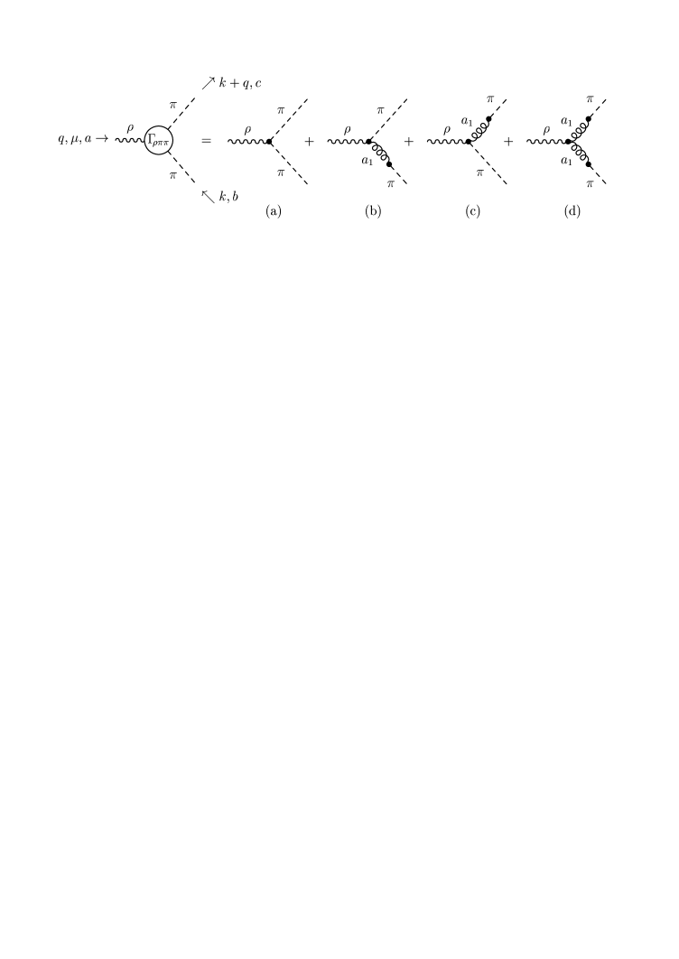
Figure 1: The $\rho\pi\pi$ vertex function of the gauged linear $\sigma$ model after symmetry breaking.

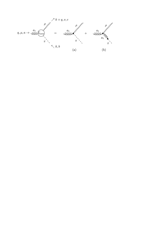
Figure 2: The ${a_{1}}\pi\rho$ vertex function of the gauged linear $\sigma$ model after symmetry breaking.

If the $\pi-{a_{1}}$ mixing is not eliminated, there are four contributions to the $\rho\pi\pi$ vertex. The corresponding vertex factors read:

$$\big{(}\Gamma_{\rho\pi\pi}^{\mathrm{(a)}}\big{)}_{abc}^{\mu} =-g\,\varepsilon_{abc}\,(2\,k^{\mu}+q^{\mu})\,,$$ (22)

$$\big{(}\Gamma_{\rho\pi\pi}^{\mathrm{(b+c)}}\big{)}_{abc}^{\mu} =\frac{g^{3}\sigma_{0}^{2}}{m_{a_{1}}^{2}}\,\varepsilon_{abc}\,(2\,k^{\mu}+q^{\mu})\,,$$ (23)

$$\big{(}\Gamma_{\rho\pi\pi}^{\mathrm{(d)}}\big{)}_{abc}^{\mu} =\frac{g^{3}\sigma_{0}^{2}}{m_{a_{1}}^{4}}\,\varepsilon_{abc}\,(q^{2}\,k^{\mu}-k\cdot q\,q^{\mu})\,.$$ (24)

The coupling constant $g$ can be determined from Eqs. (18) and (21) and the empirical values of $f_{\pi}$, $m_{\rho}$ and $m_{a_{1}}$. If we take e.g. $m_{\rho}=770\;\mathrm{MeV}$, $m_{a_{1}}\approx\sqrt{2}\,m_{\rho}=1090\;\mathrm{MeV}$ , and $f_{\pi}=93\;\mathrm{MeV}$, we find $g=5.9$ . This is more or less the value which is needed to obtain a good description of the $\rho$-meson width and the electromagnetic pion form factor in models without $a_{1}$-degrees of freedom, where the $\rho\pi\pi$ vertex function consists of diagram (a) only (see e.g. Ref. [8]). In the present model, the second contribution, (b+c), has the same structure as (a) and leads to a reduction of the $\rho\pi\pi$ coupling constant by a factor $1-g^{2}\sigma_{0}^{2}/m_{a_{1}}^{2}=m_{\rho}^{2}/m_{a_{1}}^{2}=1/Z$. However, this is exactly cancelled by the factors $\sqrt{Z}$ assigned to each external pion line if one calculates the decay $\rho\rightarrow\pi\pi$. Thus, the contributions (a) to (c) would give a quite good description of the decay $\rho\rightarrow\pi\pi$ with the value $g=5.9$ determined above. Unfortunately there is still contribution (d), which generates a strong $q^{2}$-dependence of the vertex function. This does not only result in a too small width for $\rho\rightarrow\pi\pi$, but also leads to a wrong shape of the pion electromagnetic form factor or the $\pi-\pi$ scattering phase shifts in the $J=1,I=1$ channel as a function of $q^{2}$, which can perfectly be reproduced without momentum dependence of the vertex.

A similar effect exists for the decay ${a_{1}}\rightarrow\pi\rho$. Due to $\pi-{a_{1}}$ mixing there are two contributions to the ${a_{1}}\pi\rho$ vertex function shown in Fig. 2:

$$\big{(}\Gamma_{{a_{1}}\pi\rho}^{(a)}\big{)}_{abc}^{\mu\nu} =ig^{2}\sigma_{0}\,\varepsilon_{abc}\,g^{\mu\nu}\,,$$ (25)

$$\big{(}\Gamma_{{a_{1}}\pi\rho}^{(b)}\big{)}_{abc}^{\mu\nu} =-i\frac{g^{2}\sigma_{0}}{m_{a_{1}}^{2}}\,\varepsilon_{abc}\,\big{(}k^{\mu}k^{\nu}+k^{\mu}q^{\nu}+q^{\mu}k^{\nu}-(k^{2}+2\,k\cdot q)\,g^{\mu\nu}\big{)}\,.$$ (26)

Again, the term arising from the non-abelian terms in the field strength tensors $Y_{\mu\nu}$,

$${\mathcal{L}}_{YYY}=-\frac{ig}{2}\,\mathrm{tr}\,\partial_{\mu}Y_{\nu}\,[Y^{\mu},Y^{\nu}]$$ (27)

causes an additional momentum dependence of the vertex. As a consequence, the amplitude for ${a_{1}}\rightarrow\rho\pi$ as a function of the invariant mass of the ${a_{1}}$ has a zero at $q^{2}=m_{a_{1}}^{2}+m_{\rho}^{2}$ . This lies well below the $\tau$ mass, i.e. within the range where the ${a_{1}}$ can experimentally be observed under clean conditions. The experimental data, however, show no minimum in the $\pi\rho$ invariant mass spectrum [21, 22].

2.2 Restriction to global chiral symmetry

The problems discussed in the end of the previous section force us to modify the Lagrangian, Eq. (15). To that end we relax the constraints imposed by the requirement that the Lagrangian (except for the mass term ${\cal L}_{m_{0}}$) should be invariant under a local $SU(2)_{L}\times SU(2)_{R}$ transformation and only insist on a global chiral symmetry. In fact, this has already been done in Ref. [19], but in a less radical way.

Two consequences of the gauge principle are incorporated in the Lagrangian (15): First, the same coupling constant $g$ appears in different interaction terms, and second, some chirally symmetric interaction terms are not allowed. For example, the most general interaction of two $\Phi$ fields with two $Y$ fields which is chirally symmetric and has dimension $\leq 4$ looks as follows:

$${\mathcal{L}}_{\Phi\Phi YY}=-\frac{h_{1}}{2}\,Y_{\mu}\Phi\cdot Y^{\mu}\Phi+\frac{h_{2}}{4}\,\Phi\cdot\Phi\,\mathrm{tr}\,Y_{\mu}Y^{\mu}\,.$$ (28)

The gauge principle would force us to choose $h_{1}=g^{2}$ and $h_{2}=0$, whereas in Ref. [19], $h_{1}$ and $h_{2}$ were chosen as independent parameters $h_{1}=g^{2}\,(1+2c)$ and $h_{2}=g^{2}\,(b-c)$ (with $b$ and $c$ as defined in Ref. [19]).

As we have shown in the previous section, the problems with the phenomenology of $\rho$ and ${a_{1}}$ mesons arise mainly from the vector meson self interaction. However, if we are interested only in global chiral symmetry, we can adjust the coupling constants independently:

$${\mathcal{L}}_{YYY}+{\mathcal{L}}_{YYYY}=-\frac{ig^{\prime}}{2}\,\mathrm{tr}\,\partial_{\mu}Y_{\nu}\,[Y^{\mu},Y^{\nu}]+\frac{g^{\prime\prime\,2}}{4}\,\mathrm{tr}\,Y_{\mu}Y_{\nu}\,[Y^{\mu},Y^{\nu}]\,.$$ (29)

We are allowed to choose the coupling constants $g^{\prime}$ and $g^{\prime\prime}$ smaller than $g$ or even to put them to zero. In fact, we perform our calculations with arbitrary values of these coupling constants, and find that the best description of the axial-vector correlator can be achieved with $g^{\prime}=0$, while our results are insensitive to $g^{\prime\prime}$. For simplicity, we will put both, $g^{\prime}$ and $g^{\prime\prime}$, to zero throughout this paper.

In addition to the $g^{\prime\prime}$ term, one could think of other chirally symmetric $YYYY$-interaction terms of dimension $4$. However, they are not important for our purposes, either. Higher-dimension terms, which are frequently used in the literature [18, 17, 19], are much more complicated and result in momentum dependent vertices. As we will see, the experimental data on $\rho$ and $a_{1}$ mesons can very well be explained without such terms. This indicates that in nature the momentum dependence of the vertices is small.

Besides the interaction terms, we also modify the kinetic term for the vector mesons contained in Eq. (13). With the original kinetic term, the longitudinal part of the vector meson propagator does not go to zero for $k^{2}\rightarrow\infty$, causing serious problems if one tries to calculate loop diagrams with vector meson lines. To avoid these problems, we take the Stückelberg Lagrangian [23]

$${\mathcal{L}}_{\mathrm{kin}\,Y}=-\frac{1}{8}\,\mathrm{tr}\,(\partial_{\mu}Y_{\nu}-\partial_{\nu}Y_{\mu})(\partial^{\mu}Y^{\nu}-\partial^{\nu}Y^{\mu})-\frac{\xi}{4}\,\mathrm{tr}\,(\partial_{\mu}Y^{\mu})^{2}\,.$$ (30)

From this one retrieves the kinetic term of the original Lagrangian (13) by taking the limit $\xi\rightarrow 0$ . The $\rho$ meson propagator now has the form

$$G^{\mu\nu}_{\rho}(k)=\frac{\frac{k^{\mu}k^{\nu}}{m_{\rho}^{2}}-g^{\mu\nu}}{k^{2}-m_{\rho}^{2}}-\frac{\frac{k^{\mu}k^{\nu}}{m_{\rho}^{2}}}{k^{2}-m_{\rho}^{2}/\xi}\,.$$ (31)

This form has the advantage that for $\xi>0$ the propagator behaves as $1/k^{2}$ for $k^{2}\rightarrow\infty$, which is not true for $\xi=0$. On the other hand, we have introduced unphysical scalar particles with mass $m_{\rho}/\sqrt{\xi}$. This can be interpreted as some form of regularization of the contributions from the longitudinal polarization states of the vector mesons. Therefore the parameter $\xi$ must be chosen small enough, such that all thresholds involving these unphysical particles lie above the energy range we are interested in.

Combining everything, we obtain our full Lagrangian:

$${\mathcal{L}}=\, \frac{1}{2}\,\partial_{\mu}\Phi\cdot\partial^{\mu}\Phi-\frac{\mu^{2}}{2}\,\Phi\cdot\Phi-ig\,Y_{\mu}\Phi\cdot\partial^{\mu}\Phi-\frac{h_{1}}{2}\,Y_{\mu}\Phi\cdot Y^{\mu}\Phi+\frac{h_{2}}{4}\,\Phi\cdot\Phi\,\mathrm{tr}\,Y_{\mu}Y^{\mu}$$

$$-\frac{\lambda^{2}}{4}\,(\Phi\cdot\Phi)^{2}+c\sigma-\frac{1}{8}\,\mathrm{tr}\,(\partial_{\mu}Y_{\nu}-\partial_{\nu}Y_{\mu})(\partial^{\mu}Y^{\nu}-\partial^{\nu}Y^{\mu})-\frac{\xi}{4}\,\mathrm{tr}\,(\partial_{\mu}Y^{\mu})^{2}$$

$$+\frac{m_{0}^{2}}{4}\,\mathrm{tr}\,Y_{\mu}Y^{\mu}\,.$$ (32)

Again, as in the previous section, we must shift the $\sigma$ field, and Eqs. (16) and (17) remain valid. But instead of Eq. (18) we find the following expressions for the meson masses:

$$m_{\pi\,{0}}^{2}=\mu^{2}+\lambda^{2}\sigma_{0}^{2}\,,\quad m_{\sigma}^{2}=\mu^{2}+3\lambda^{2}\sigma_{0}^{2}\,,\quad m_{\rho}^{2}=m_{0}^{2}+h_{2}\,\sigma_{0}^{2}\,,\quad m_{a_{1}}^{2}=m_{0}^{2}+(h_{1}+h_{2})\,\sigma_{0}^{2}\,.$$ (33)

This has the interesting consequence that with a special choice of parameters ($m_{0}=0$, $h_{2}=m_{\rho}^{2}/\sigma_{0}^{2}$) it is now possible to generate the vector meson masses from chiral symmetry breaking alone. In this case the masses of both $\rho$ and ${a_{1}}$ meson would drop in a nuclear medium where chiral symmetry is (partially) restored (“Brown–Rho scaling” [4]).

The $\pi-{a_{1}}$ mixing Lagrangian ${\mathcal{L}}_{\pi{a_{1}}}$ is still given by Eq. (19), but because of the Stückelberg ($\xi$-) term in the Lagrangian it cannot be eliminated by a simple field redefinition. Instead, self-energy contributions from ${\mathcal{L}}_{\pi{a_{1}}}$ must be iterated to all orders as shown in Fig. 3(a).

Figure 3: Propagators with $\pi-{a_{1}}$ mixing: (a) the pion propagator $iG_{\pi}(k)$, (b) the ${a_{1}}$ propagator $iG_{{a_{1}}}^{\mu\nu}(k)$, and (c) the mixed propagator $iG_{\pi{a_{1}}}^{\mu}(k)$.

Then the pion propagator can be written as

$$G_{\pi}(k)=\frac{1}{k^{2}-m_{\pi\,{0}}^{2}+\frac{g^{2}\sigma_{0}^{2}k^{2}}{\xi k^{2}-m_{a_{1}}^{2}}}=\sum_{i=1}^{2}\frac{Z_{\pi\,{i}}}{k^{2}-m_{\pi\,{i}}^{2}}\,.$$ (34)

The first pole at $m_{\pi\,{1}}=m_{\pi}$ corresponds to the physical pion, whereas the second one at $m_{\pi\,{2}}$ corresponds to the unphysical longitudinally polarized ${a_{1}}$ particle. In principle $m_{\pi\,{1}}$ and $m_{\pi\,{2}}$ are functions of $m_{\pi\,{0}}$ , but it is more convenient to quote the relations for these masses as functions of the physical pion mass:

$$m_{\pi\,{1}}^{2}=m_{\pi}^{2}\,,\quad m_{\pi\,{2}}^{2}=\frac{m_{a_{1}}^{2}(m_{a_{1}}^{2}-g^{2}\sigma_{0}^{2}-\xi m_{\pi}^{2})}{\xi(m_{a_{1}}^{2}-\xi m_{\pi}^{2})}\,,\quad m_{\pi\,{0}}^{2}=\frac{m_{\pi}^{2}(m_{a_{1}}^{2}-g^{2}\sigma_{0}^{2}-\xi m_{\pi}^{2})}{m_{a_{1}}^{2}-\xi m_{\pi}^{2}}\,.$$ (35)

The $Z_{\pi\,{i}}$ are given by

$$Z_{\pi\,{1}}=\frac{m_{a_{1}}^{2}-\xi m_{\pi\,{1}}^{2}}{\xi(m_{\pi\,{2}}^{2}-m_{\pi\,{1}}^{2})}\,,\qquad Z_{\pi\,{2}}=1-Z_{\pi\,{1}}\,.$$ (36)

Here $Z_{\pi\,{1}}$ corresponds to the $Z$ factor introduced in the previous section. In the limit $\xi\rightarrow 0$, $h_{1}\rightarrow g^{2}$ and $h_{2}\rightarrow 0$ we retrieve the relations for $m_{\pi}$, $m_{\pi\,{0}}$ and $Z$ in the gauged linear sigma model.

The ${a_{1}}$ and the mixed ($\pi-{a_{1}}$) propagator can be obtained from the pion propagator as shown in Figs. 3(b) and (c). For the ${a_{1}}$ propagator we find

$$G_{{a_{1}}}^{\mu\nu}(k)=\frac{\frac{k^{\mu}k^{\nu}}{m_{a_{1}}^{2}}-g^{\mu\nu}}{k^{2}-m_{a_{1}}^{2}}+k^{\mu}k^{\nu}\sum_{i=1}^{2}\frac{Z_{a_{1}\,{i}}}{k^{2}-m_{\pi\,{i}}^{2}}\,,$$ (37)

with

$$Z_{a_{1}\,{1}}=\frac{m_{\pi\,{1}}^{2}-m_{\pi\,{0}}^{2}}{\xi m_{\pi\,{1}}^{2}(m_{\pi\,{2}}^{2}-m_{\pi\,{1}}^{2})}\,,\qquad Z_{a_{1}\,{2}}=-\frac{1}{m_{a_{1}}^{2}}-Z_{a_{1}\,{1}}\,,$$ (38)

and for the mixed propagator

$$G_{\pi{a_{1}}}^{\mu}(k)=ik^{\mu}\sum_{i=1}^{2}\frac{Z_{\pi a_{1}\,{i}}}{k^{2}-m_{\pi\,{i}}^{2}}\,,$$ (39)

with

$$Z_{\pi a_{1}\,{1}}=-\frac{g\sigma_{0}}{\xi(m_{\pi\,{2}}^{2}-m_{\pi\,{1}}^{2})}\,,\qquad Z_{\pi a_{1}\,{2}}=-Z_{\pi a_{1}\,{1}}\,.$$ (40)

Since we have switched off the 3-vector interaction, for the $\rho\pi\pi$ vertex functions only the diagrams (a) to (c) of Fig. 1 are left. If the external pions are on-shell, i.e. $k^{2}=(k+q)^{2}=m_{\pi}^{2}$ , the total vertex function reads,

$$\big{(}\Gamma_{\rho\pi\pi}\big{)}_{abc}^{\mu}=-\Big{(}g-\frac{h_{1}\sigma_{0}^{2}}{m_{a_{1}}^{2}-\xi m_{\pi}^{2}}\Big{)}\,\varepsilon_{abc}\,(2\,k^{\mu}+q^{\mu})\,.$$ (41)

This can be used to define an effective $\rho\pi\pi$ coupling constant

$$g_{\rho\pi\pi}^{\mathrm{eff}}=\Big{(}g-\frac{h_{1}\sigma_{0}^{2}}{m_{a_{1}}^{2}-\xi m_{\pi}^{2}}\Big{)}Z_{\pi\,{1}}=g\frac{(m_{\rho}^{2}-\xi m_{\pi}^{2})(m_{a_{1}}^{2}-\xi m_{\pi}^{2})}{(m_{a_{1}}^{2}-\xi m_{\pi}^{2})^{2}-g^{2}\sigma_{0}^{2}m_{a_{1}}^{2}}\,.$$ (42)

2.3 Electroweak interactions

Until now we have completely neglected the electroweak interaction. However, the cleanest experimental information about $\rho$ and ${a_{1}}$ mesons can be obtained from electromagnetic reactions, $e^{+}e^{-}\rightarrow\rho$, and from the weak decay of the $\tau$ lepton, $\tau\rightarrow\nu_{\tau}\,\rho$ or $\tau\rightarrow\nu_{\tau}\,{a_{1}}$. Another reason why we want to include the electromagnetic interactions is of course our interest in dilepton production in heavy ion collisions.

At the quark level there is no ambiguity how the electromagnetic field and the $W$ bosons must be introduced: The ordinary derivative of the quark fields is replaced by a covariant derivative. If we consider only $u$ and $d$ quarks ($\psi=(u,d)$), this looks as follows (see e.g. [24]):

$$D_{\mu}\psi=\Big{(}\partial_{\mu}-ie\,A_{\mu}\,\frac{\tau_{3}}{2}-\frac{ie\cos\theta_{C}}{\sin\theta_{W}}\,\frac{1-\gamma_{5}}{2}\,\Big{(}W_{1\,\mu}\frac{\tau_{1}}{2}+W_{2\,\mu}\frac{\tau_{2}}{2}\Big{)}+\dots\Big{)}\psi\,\,.$$ (43)

Here we have omitted the isoscalar part of the electromagnetic interaction and the $Z$ boson coupling, since they are irrelevant for our purposes.

This can be generalized to the $(\sigma,\vec{\pi})$ meson sector. The isospin operator $\vec{\tau}/2$ corresponds to the $\vec{T}$ operator, whereas $\gamma_{5}\vec{\tau}/2$ can be identified with $\vec{T}^{5}$. Therefore all derivatives $\partial_{\mu}\Phi$ in the Lagrangian (32) have to be replaced by

$$D_{\mu}\Phi =\Big{(}\partial_{\mu}-ie\,A_{\mu}T_{3}-\frac{ie\cos\theta_{C}}{\sin\theta_{W}}\,(W_{1\,\mu}T^{L}_{1}+W_{2\,\mu}T^{L}_{2})\Big{)}\Phi$$

$$=\begin{pmatrix}\partial_{\mu}\,\sigma\\ \partial_{\mu}\,\vec{\pi}\end{pmatrix}+e\begin{pmatrix}0\\ \vec{A}_{\mu}\times\vec{\pi}\end{pmatrix}+\frac{e\cos\theta_{C}}{2\sin\theta_{W}}\begin{pmatrix}-\vec{W}_{\mu}\cdot\vec{\pi}\\ \vec{W_{\mu}}\times\vec{\pi}+\vec{W}_{\mu}\,\sigma\end{pmatrix}\,.$$ (44)

In the last line we have used the abbreviations

$$\vec{A}_{\mu}=\begin{pmatrix}0\\ 0\\ A_{\mu}\end{pmatrix}\,,\qquad\vec{W}_{\mu}=\begin{pmatrix}W_{1\,\mu}\\ W_{2\,\mu}\\ 0\end{pmatrix}\,.$$ (45)

To find the operators in the vector-meson space corresponding to the $\vec{T}$ and $\vec{T}^{5}$ operators in the $(\sigma,\vec{\pi})$-meson space, we can expand Eq. (10) for the case $\partial_{\mu}U=0$ to linear order in $\vec{\alpha}$ and $\vec{\beta}$. Then it becomes clear that the derivatives of the vector meson fields, $\partial_{\mu}Y_{\nu}$ , must be changed into

$$D_{\mu}Y_{\nu} =\partial_{\mu}Y_{\nu}-ie\,A_{\mu}\,[T_{3}\,,Y_{\nu}]-\frac{ie\cos\theta_{C}}{\sin\theta_{W}}\,(W_{1\,\mu}\,[T^{L}_{1}\,,Y_{\nu}]+W_{2\,\mu}\,[T^{L}_{2}\,,Y_{\nu}])$$

$$=:D_{\mu}\vec{\rho}_{\nu}\cdot\vec{T}+D_{\mu}\vec{a}_{1\,\nu}\cdot\vec{T}^{5}\,,$$ (46)

with

$$D_{\mu}\vec{\rho}_{\nu} =\partial_{\mu}\,\vec{\rho}_{\nu}+e\,\vec{A}_{\mu}\times\vec{\rho}_{\nu}+\frac{e\cos\theta_{C}}{2\sin\theta_{W}}\,\vec{W}_{\mu}\times(\vec{\rho}_{\nu}-\vec{a}_{1\,\nu})\,,$$

$$D_{\mu}\vec{a}_{1\,\nu} =\partial_{\mu}\,\vec{a}_{1\,\nu}+e\,\vec{A}_{\mu}\times\vec{a}_{1\,\nu}+\frac{e\cos\theta_{C}}{2\sin\theta_{W}}\,\vec{W}_{\mu}\times(\vec{a}_{1\,\nu}-\vec{\rho}_{\nu})\,.$$ (47)

One should mention that the replacements described above must be made before the redefinition of the $\sigma$ field, Eq. (16). When we now perform the shift of the $\sigma$ field, $W-\pi$ and $W-{a_{1}}$ couplings emerge. As a consequence there are two contributions to the pion decay, a direct one and a contribution with an intermediate longitudinal $a_{1}$:

$$f_{\pi}=\sqrt{Z_{\pi\,{1}}}\Big{(}\sigma_{0}-\frac{g^{2}\sigma_{0}^{3}}{m_{a_{1}}^{2}-\xi\,m_{\pi\,{1}}^{2}}\Big{)}=\frac{\sigma_{0}\,(m_{a_{1}}^{2}-\xi m_{\pi}^{2}-g^{2}\sigma_{0}^{2})}{\sqrt{(m_{a_{1}}^{2}-\xi m_{\pi}^{2})^{2}-g^{2}\sigma_{0}^{2}m_{a_{1}}^{2}}}\,.$$ (48)

Obviously we did not assume anything about vector meson dominance when we constructed the coupling of the $A$ and $W$ fields to the mesons, and in principle the vector mesons were not treated differently from the scalar mesons. Hence, the $A$ and $W$ fields simply couple to the Noether currents. In addition there are seagull terms involving two $A$ or $W$ fields. At this stage there is no direct $\gamma-\rho$ or $W-\rho$ coupling in our model. However, as we will see in Sect. 4.1, the $\gamma-\rho$ and $W-\rho$ coupling appears naturally at the one-loop level, where we will need a counterterm of the form

$${\mathcal{L}}_{\gamma Y}+{\mathcal{L}}_{WY}=-\frac{f}{4}\,\mathrm{tr}\,(\partial_{\mu}Y_{\nu}-\partial_{\nu}Y_{\mu})\,\partial^{\mu}\,\Big{(}eA^{\nu}T_{3}+\frac{e\cos\theta_{C}}{\sin\theta_{W}}\,(W_{1}^{\nu}T_{1}^{L}+W_{2}^{\nu}T_{2}^{L})\Big{)}\,.$$ (49)

The $\gamma-\rho$ part of this term has exactly the form of the $\gamma-\rho$ coupling of Kroll, Lee and Zumino [25],

$${\mathcal{L}}_{\gamma\rho}=-\frac{ef}{2}\,(\partial_{\mu}\rho_{3\,\nu}-\partial_{\nu}\rho_{3\,\mu})(\partial^{\mu}A^{\nu}-\partial^{\nu}A^{\mu})\,,$$ (50)

the only difference being that in Ref. [25] the coupling constant $f$ was fixed to $1/g$, whereas it is a free parameter in our model.

3 Meson propagators in one-loop approximation

Our aim is the chirally symmetric description of the vector isovector and axial-vector isovector correlation functions. This implies that we need a chirally symmetric description of $\rho$ and ${a_{1}}$ mesons. By construction, our Lagrangian is chirally symmetric, but most approximations beyond tree-level destroy the symmetry. For example, in the linear $\sigma$ model without vector mesons the mean field (Hartree-Fock) approximation violates the Goldstone theorem, which can be recovered only if one includes also the RPA corrections [26]. Then, of course, the self-consistency is lost, i.e. the final RPA mesons are different from the mean-field mesons propagating in the loops. In fact, a more general investigation of this problem shows that there seems to be no self-consistent approximation scheme which respects the symmetry at the correlator level [27].

A simple symmetry conserving approximation scheme is given by a loop expansion, which formally corresponds to an expansion in powers of $\hbar$. Here we will calculate the meson self energies to one-loop order. This approximation has the following properties:

1. The pion remains massless in the chiral limit (Goldstone theorem).

2. All differences of chiral partners ($\pi-\sigma$ and $\rho-{a_{1}}$) disappear when the chiral symmetry is restored ($\sigma_{0}=0$).

3. The dominant meson decay modes, such as $\rho\rightarrow\pi\pi$ or ${a_{1}}\rightarrow\pi\rho$, are contained in the scheme. Of course, due to the lack of self-consistency the final decay of the $\rho$ meson in ${a_{1}}\rightarrow\pi\rho\rightarrow\pi\pi\pi$ is not included.

Of course, in a strongly interacting theory the loop expansion does not converge. Therefore the model is not defined by its Lagrangian alone, but only by the Lagrangian together with the approximation scheme used. Hence the propagators and vertices obtained from the Lagrangian must not be interpreted as elementary, but rather as parametrizations of the full propagators and vertices, containing all non-perturbative effects which are not explicitly taken into account in the approximation scheme.

3.1 Subtraction of divergences

If one calculates diagrams with loops, one always finds divergent expressions which have to be regularized in some way. The above mentioned fact, that the vertices and propagators obtained from our Lagrangian are not elementary, justifies the introduction of form factors, which are frequently used in the literature in order to cut off high momenta [7, 9, 30], rendering the loop integrals finite. These form factors are independent parameters and cannot be computed from the Lagrangian. Unfortunately we cannot simply attach form factors to the vertices obtained from our Lagrangian, since this would destroy the symmetry properties of our model.

Other regularization prescriptions, which can be found in the literature, are the Pauli-Villars scheme with finite regulator mass [8] or subtracted dispersion relations. Using these prescriptions one can sometimes avoid the problems arising from form factors, although they give very similar results. As an example consider the self-energy $\Sigma_{\rho\rightarrow\pi\pi}$, describing the decay of the $\rho$ meson into two pions, with a three dimensional form factor $v(\vec{k})$ attached to each $\rho\pi\pi$ vertex, which cuts off pion momenta $\vec{k}$ (measured in the $\rho$-meson rest frame) at some value $|\vec{k}|_{\mathrm{max}}$ . For small $\rho$-meson energies, $q^{2}\lesssim 4(m_{\pi}^{2}+\vec{k}_{\mathrm{max}}^{2})$, the imaginary part of $\Sigma_{\rho\rightarrow\pi\pi}$ is not modified by the form factor. For the real part the situation is more complicated. Since it is related to the imaginary part via a dispersion integral, it receives already for low $q^{2}$ contributions from the imaginary part at high $q^{2}$. Therefore it depends strongly on $|\vec{k}|_{\mathrm{max}}$. However, using subtracted dispersion relations, one can easily convince oneself that for low energies the influence of the form factor on the real part can approximately be absorbed in the subtraction constants, while the remaining dispersion integral is almost independent of the form factor.

In this sense, subtracted dispersion relations can be interpreted as an approximate way of attaching form factors to the vertices. As the subtraction constants depend on the high-energy behavior of the form factors, they cannot be calculated from the Lagrangian, but they are free parameters. However, there are some contraints which follow from chiral symmetry. In order to preserve the symmetry, we must make equal subtractions from the self energies of chiral partners. Obviously this is mathematically ill-defined, since the subtractions are infinite. Therefore we need a more systematic method to ensure the consistency of the subtractions.

The subtractions can be regarded as (infinite) counterterms added to the original Lagrangian. Thus the subtractions are consistent with chiral symmetry if the counterterms are chirally invariant. The values of the counterterms are determined as follows [28]. First we calculate the self-energy diagrams with dimensional regularization, i.e. we calculate the loop integrals in $d$ space-time dimensions,

$$\int\frac{d^{4}{k}}{(2\pi)^{4}}\,\cdots\longrightarrow\int\frac{d^{d}{k}}{(2\pi)^{d}}\,\Big{(}\frac{\Lambda^{2}}{4\pi}\Big{)}^{\frac{4-d}{2}}\,\cdots\,.$$ (51)

If we expand the result in the vicinity of $d=4$, the divergences appear as poles $\propto 1/(4-d)$. The residues of these poles are mathematically well-defined, and the self energy can be written in the form

$$\Sigma=\overline{\Sigma}+\Sigma_{\infty}\,\Big{(}\frac{1}{4-d}-\frac{\gamma}{2}\Big{)}\,.$$ (52)

In this way we have split the self energy into a finite part $\overline{\Sigma}$, and an infinite part. ($\gamma=0.577\ldots=$ Euler’s constant is finite, but it is convenient to keep the infinite $1/(4-d)$ term and the $\gamma/2$ term together.) The counterterms are also split into finite and infinite parts, e.g. $\delta\mu^{2}=\overline{\delta\mu^{2}}+\delta\mu^{2}_{\infty}(1/(4-d)-\gamma/2)$. The infinite parts of the counterterms must be adjusted such that $\Sigma_{\infty}$ vanishes, while the finite parts are treated as free parameters. The crucial point is that each counterterm may be adjusted only once and not separately for different self energies.

The factor $(\Lambda^{2}/(4\pi))^{(4-d)/2}$ in Eq. (51) ensures that the dimension of the result does not depend on $d$. The finite parts of the integrals, of course, depend on the choice of $\Lambda$. However, the physical results are independent of $\Lambda$, if the finite parts of the counterterms are appropriately readjusted after a change of $\Lambda$. For example, if $\Lambda$ is changed to $\Lambda^{\prime}$, $\overline{\delta\mu^{2}}$ must be changed to $\overline{\delta\mu^{2}}+\delta\mu^{2}_{\infty}\ln(\Lambda^{\prime}/\Lambda)$.

3.2 The tadpole correction

At tree level, no $\sigma$ line can disappear into the vacuum, because all terms linear in $\sigma$ are eliminated by the shift of the $\sigma$ field, Eq. (16), as a consequence of Eq. (17), which can be illustrated diagrammatically as shown in Fig. 4(a).

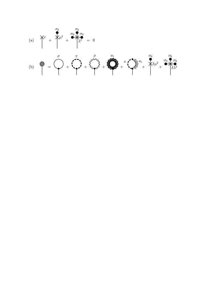
Figure 4: (a) Diagrammatic illustration of Eq. (17), which shows that there are no tadpole graphs at tree level. (b) Tadpole graphs $T$ at one-loop order. The meaning of thick and thin lines is the same as in Fig. 3.

This is no longer true at the one-loop level, where one has the additional tadpole graphs shown in Fig. 4(b). The last two contributions are generated by the chirally symmetric counterterms

$$\delta{\mathcal{L}}_{\mu^{2}}+\delta{\mathcal{L}}_{\lambda^{2}}=-\frac{\delta\mu^{2}}{2}\Phi\cdot\Phi-\frac{\delta\lambda^{2}}{4}(\Phi\cdot\Phi)^{2}\,.$$ (53)

Calculating the diagrams displayed in Fig. 4(b) and splitting the result into finite and infinite parts, $T=\overline{T}+T_{\infty}(1/(4-d)-\gamma/2)$, we find for the infinite part

$$T_{\infty}=\, \frac{3i\sigma_{0}}{8\pi^{2}}\Big{(}\frac{(h_{1}+2h_{2}-g^{2})m_{0}^{2}}{\xi^{2}}-\frac{g^{2}\mu^{2}}{\xi}+(3h_{1}+6h_{2})m_{0}^{2}+2\lambda^{2}\mu^{2}\Big{)}$$

$$+\frac{3i\sigma_{0}^{3}}{8\pi^{2}}\Big{(}\frac{(h_{1}+h_{2}-g^{2})^{2}+h_{2}^{2}}{\xi^{2}}-\frac{2g^{2}(h_{1}+h_{2})}{\xi}+3(h_{1}+h_{2})^{2}+3h_{2}^{2}+4\lambda^{2}\Big{)}$$

$$-i\sigma_{0}\delta\mu^{2}_{\infty}-i\sigma_{0}^{3}\delta\lambda^{2}_{\infty}\,.$$ (54)

From this one can immediately see that $T$ can be made finite (i.e. $T_{\infty}=0$) by a proper choice of $\delta\mu^{2}_{\infty}$ and $\delta\lambda^{2}_{\infty}$ . Furthermore, this choice does not depend on $c$ or $\sigma_{0}$, i.e. on the explicit or spontaneous symmetry breaking. In the following sections we will see that this is a general property of all counterterms, as shown by Lee [29] for the linear $\sigma$ model without vector mesons and by Ram Mohan [28] for the linear $\sigma$ model with nucleons at finite temperature and density. In this context we should remark that, in the limit $\xi\rightarrow 0$, it is impossible to find suitable counterterms independent of $\sigma_{0}$ . For example, the third contribution in Fig. 4(b) can be written as

$$-3h_{2}\,\sigma_{0}\,g_{\mu\nu}\int\frac{d^{4}{k}}{(2\pi)^{4}}\,G_{\rho}^{\mu\nu}(k) =3h_{2}\,\sigma_{0}\int\frac{d^{4}{k}}{(2\pi)^{4}}\,\Big{(}\frac{3}{k^{2}-m_{\rho}^{2}}+\frac{1}{\xi k^{2}-m_{\rho}^{2}}\Big{)}$$

$$=3\sum_{n=1}^{\infty}h_{2}^{n}\,\sigma_{0}^{2n-1}\int\frac{d^{4}{k}}{(2\pi)^{4}}\,\Big{(}\frac{3}{(k^{2}-m_{0}^{2})^{n}}+\frac{1}{(\xi k^{2}-m_{0}^{2})^{n}}\Big{)}\,.$$ (55)

For $\xi>0$ the $n=1$ and $n=2$ terms are quadratically and logarithmically divergent, respectively, while all terms with $n>2$ are finite. This is the reason why two counterterms independent of $\sigma_{0}$ are sufficient to cancel the divergences. In contrast, for $\xi=0$, all terms are quartically divergent, i.e. one needs either an infinite number of counterterms independent of $\sigma_{0}$ , or counterterms which depend on $\sigma_{0}$ .

3.3 The $\rho$-meson self energy

In Fig. 5 all one-loop diagrams for the $\rho$-meson self energy are displayed.

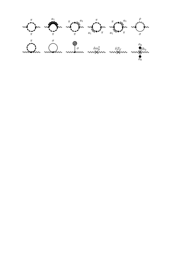
Figure 5: One-loop contributions to the $\rho$-meson self energy, $-i\Sigma_{\rho}$ .

The last three diagrams correspond to the contributions of the three counterterms which are needed to cancel the divergences:

$$\delta{\mathcal{L}}_{m_{0}^{2}}+\delta{\mathcal{L}}_{Z_{Y}}+\delta{\mathcal{L}}_{h_{2}}=\, \frac{\delta m_{0}^{2}}{4}\,\mathrm{tr}\,Y_{\mu}Y^{\mu}+\frac{\delta Z_{Y}}{8}\,\mathrm{tr}\,(\partial_{\mu}Y_{\nu}-\partial_{\nu}Y_{\mu})(\partial^{\mu}Y^{\nu}-\partial^{\nu}Y^{\mu})$$

$$+\frac{\delta h_{2}}{4}\,\Phi\cdot\Phi\,\mathrm{tr}\,Y_{\mu}Y^{\mu}$$ (56)

Again, the self energy is split into finite and infinite parts, $\Sigma_{\rho}^{\mu\nu}=\overline{\Sigma}_{\rho}^{\mu\nu}+\Sigma_{\rho\infty}^{\mu\nu}(1/(4-d)-\gamma/2)$, and the infinite parts of the counterterms are chosen such that $\Sigma_{\rho\infty}^{\mu\nu}$ vanishes .

Since in our model the $\rho$ meson is not a gauge boson, the $\rho$-meson self energy is not transverse. Instead, it can be decomposed into transverse and longitudinal components,

$$\Sigma_{\rho}^{\mu\nu}(q)=\Sigma_{\rho}^{t}(q^{2})\Big{(}\frac{q^{\mu}q^{\nu}}{q^{2}}-g^{\mu\nu}\Big{)}+\Sigma_{\rho}^{l}(q^{2})\frac{q^{\mu}q^{\nu}}{q^{2}}\,.$$ (58)

As we will see, the longitudinal part does not contribute to the vector current correlator as a consequence of current conservation.

3.4 The pion and ${a_{1}}$-meson self energies

Because of the $\pi-{a_{1}}$ mixing, the situation for the pion is a bit more complicated than for the $\rho$ meson. It is necessary to distinguish between the one-particle irreducible (1PI) self energy $\Sigma_{\pi\pi}$ , which cannot be cut into two parts by cutting any single line, and the proper self energy $\Sigma_{\pi}$ , which cannot be cut into two parts by cutting a single pion line, but which can possibly be cut into two parts by cutting a single ${a_{1}}$-meson line (see e.g. the last diagram in Fig. 3(a)).

For the ${a_{1}}$ meson the situation is similar. Here we have to distinguish between the 1PI self energy $\Sigma_{{a_{1}}{a_{1}}}$ , which cannot be cut into two parts by cutting any single line, and the proper self energy $\Sigma_{{a_{1}}}$ , which cannot be cut into two parts by cutting a single ${a_{1}}$-meson line, but which can possibly be cut into two parts by cutting a single pion line.

In Fig. 6 we display the one-loop contributions to the 1PI pion

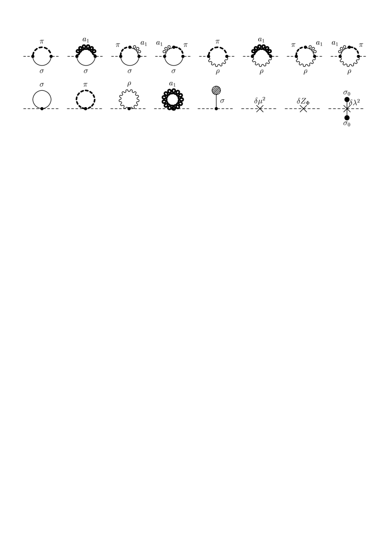
Figure 6: One-loop contributions to the 1PI pion self energy, $-i\Sigma_{\pi\pi}$ .

self energy $\Sigma_{\pi\pi}$ . The last three diagrams are generated by the counterterms given in Eq. (53) and the additional wave-function renormalization counterterm,

$$\delta{\mathcal{L}}_{Z_{\Phi}}=-\frac{\delta Z_{\Phi}}{2}\partial_{\mu}\Phi\cdot\partial^{\mu}\Phi\,.$$ (59)

One can explicitly show that this self energy fulfills the Goldstone theorem, i.e.

$$\Sigma_{\pi\pi}(0)=0\quad\mathrm{for}\quad c=0\,.$$ (60)

In particular, it is interesting to see that in the chiral limit the contributions from the $\delta\mu^{2}$ and $\delta\lambda^{2}$ counterterms ($14^{\mathrm{th}}$ and $16^{\mathrm{th}}$ diagram) exactly cancel the counterterm contributions contained in the tadpole correction ($13^{\mathrm{th}}$ diagram).

The one-loop diagrams for the 1PI ${a_{1}}$-meson self energy $\Sigma_{{a_{1}}{a_{1}}}^{\mu\nu}$ are displayed in Fig. 7.

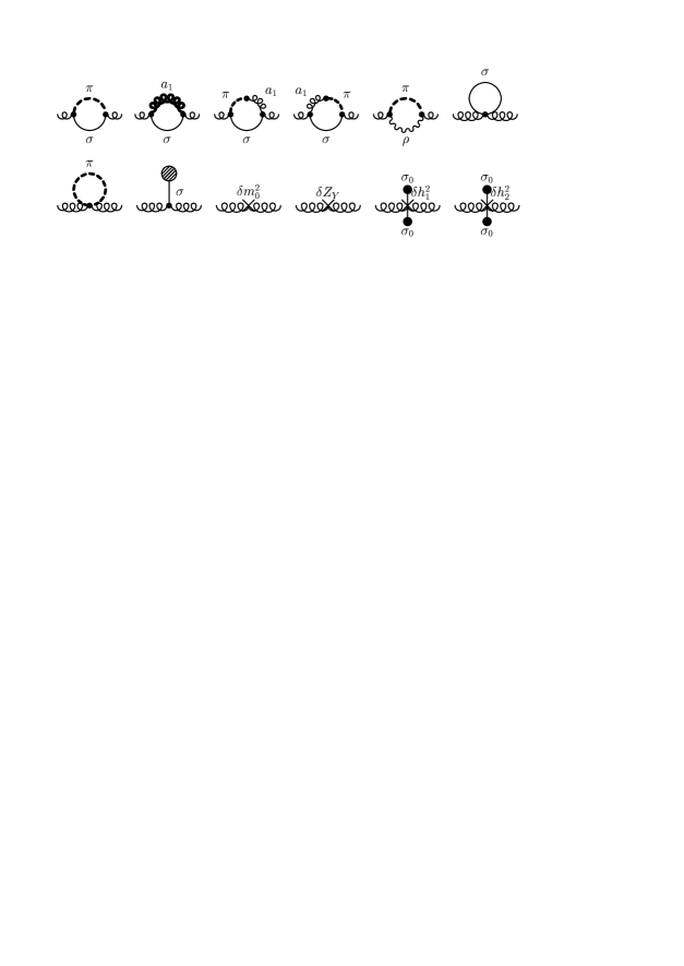
Figure 7: One-loop contributions to the 1PI ${a_{1}}$-meson self energy, $-i\Sigma_{{a_{1}}{a_{1}}}$ .

The diagrams 9, 10 and 12 are generated by the counterterms given in Eq. (56). In addition we need one more counterterm, namely

$$\delta{\mathcal{L}}_{h_{1}}=-\frac{\delta h_{1}}{2}\,Y_{\mu}\Phi\cdot Y^{\mu}\Phi\,,$$ (61)

which gives rise to the $11^{\mathrm{th}}$ diagram. In analogy to the $\rho$-meson self energy (cf. Eq. (58)), the ${a_{1}}$-meson self energy can be decomposed into transverse and longitudinal components, $\Sigma_{{a_{1}}{a_{1}}}^{t}$ and $\Sigma_{{a_{1}}{a_{1}}}^{l}$. The transverse part is not modified by $\pi-{a_{1}}$ mixing, and therefore the proper transverse ${a_{1}}$-meson self energy is equal to the 1PI transverse self energy,

$$\Sigma_{{a_{1}}}^{t}(q^{2})=\Sigma_{{a_{1}}{a_{1}}}^{t}(q^{2})\,.$$ (62)

To obtain the proper pion self energy, we have to consider also the 1PI mixed self energy $\Sigma_{\pi{a_{1}}}^{\mu}$, which is a correction to the $\pi-{a_{1}}$ vertex given by the Lagrangian (19). The corresponding one-loop diagrams are shown in Fig. 8.

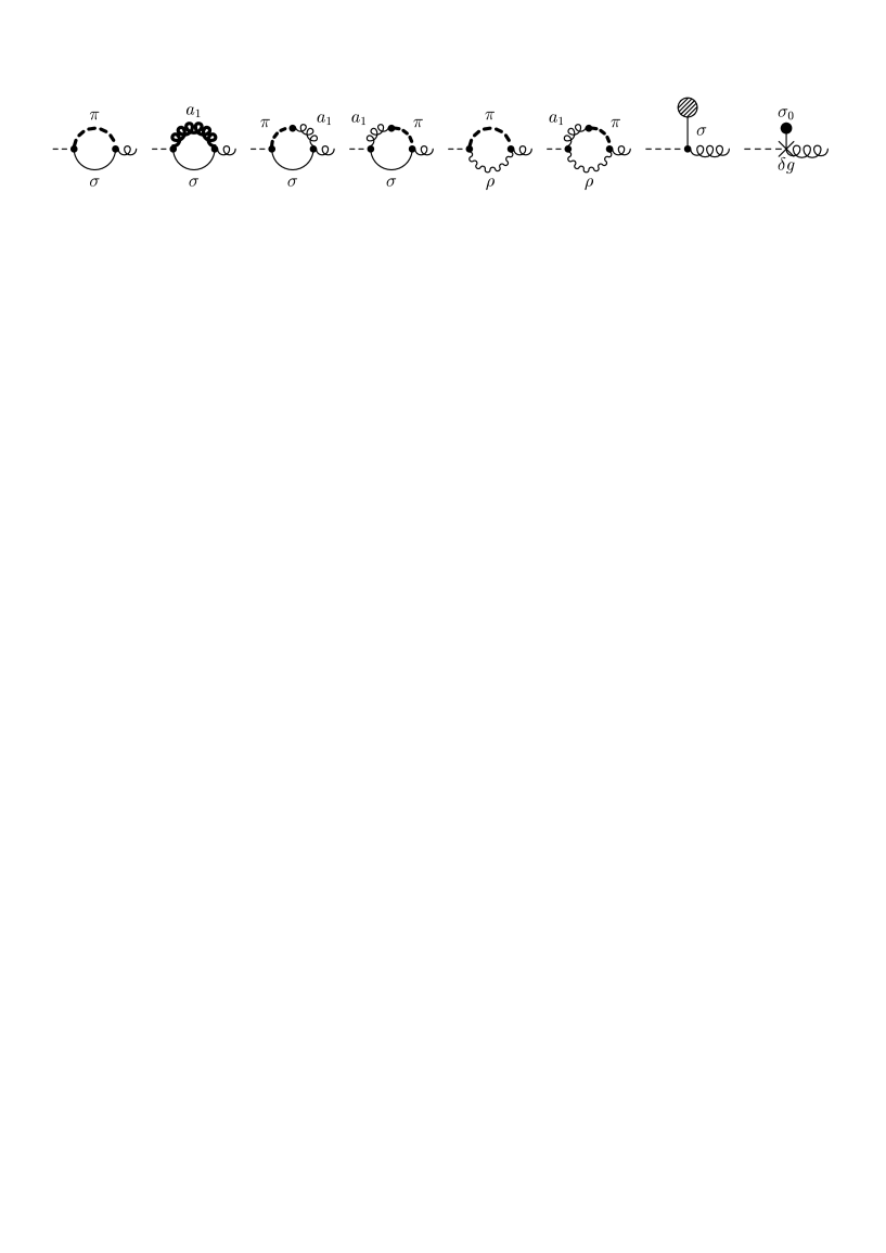
Figure 8: One-loop diagrams for the 1PI mixed $\pi-{a_{1}}$ self energy, $-i\Sigma_{\pi{a_{1}}}^{\mu}$.

The last diagram comes from the counterterm

$$\delta{\mathcal{L}}_{g}=-i\delta g\,Y_{\mu}\Phi\cdot\partial^{\mu}\Phi\,.$$ (63)

With this mixed self energy, the corrected $\pi-{a_{1}}$ mixing vertex is given by

$$\big{(}\Gamma_{\pi{a_{1}}}(q)\big{)}_{ab}^{\mu}=-\delta_{ab}\big{(}g\sigma_{0}\,q^{\mu}+i\Sigma_{\pi{a_{1}}}^{\mu}(q)\big{)}=:-q^{\mu}\delta_{ab}\,F_{\pi{a_{1}}}(q^{2})\,,$$ (64)

where $q$ is the incoming momentum of the pion. The proper pion self energy contains the tree-level self energy shown in Fig. 3(a) and the loop corrections, i.e.

$$\Sigma_{\pi}(q^{2})=\Sigma_{\pi\pi}(q^{2})+\frac{q^{2}\big{(}F_{\pi{a_{1}}}(q^{2})\big{)}^{2}}{m_{a_{1}}^{2}-\xi q^{2}-\Sigma_{{a_{1}}{a_{1}}}^{l}(q^{2})}\,.$$ (65)

The corrected pion propagator is given by $G_{\pi}^{(1)}=1/(q^{2}-m_{\pi\,{0}}^{2}-\Sigma_{\pi})$. It is obvious that $\Sigma_{\pi}$ fulfills the Goldstone theorem if $\Sigma_{\pi\pi}$ does, because the contributions due to $\pi-{a_{1}}$ mixing are proportional to $q^{2}$.

3.5 The $\sigma$-meson self energy

The self energy of the $\sigma$-meson, $\Sigma_{\sigma}$, is given by the diagrams shown in Fig. 9.

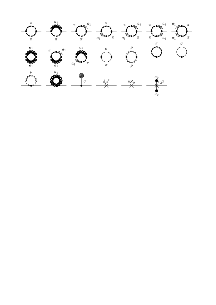
Figure 9: One-loop contributions to the $\sigma$-meson self energy, $-i\Sigma_{\sigma}$ .

To make it finite, the counterterms $\delta\mu^{2}$, $\delta\lambda^{2}$ and $\delta Z_{\Phi}$, introduced already in the previous sections, are sufficient.

4 Vector and axial-vector correlation functions

Let $\vec{j}_{\mu}$ and $\vec{j}^{5}_{\mu}$ be the hadronic vector isovector and axial-vector isovector currents, respectively. In terms of quark fields $\psi=(u,d)$ these currents read $\vec{j}_{\mu}=\overline{\psi}\gamma_{\mu}\vec{\tau}\psi/2$ and $\vec{j}^{5}_{\mu}=\overline{\psi}\gamma_{\mu}\gamma_{5}\vec{\tau}\psi/2$. The current-current correlation functions are defined by

$$\Pi_{V\,ab}^{\mu\nu}(q) =i\int d^{4}x\,e^{iq\cdot x}\langle 0|T\big{(}j_{a}^{\mu}(x)j_{b}^{\nu}(0)\big{)}|0\rangle\,,$$ (66)

$$\Pi_{A\,ab}^{\mu\nu}(q) =i\int d^{4}x\,e^{iq\cdot x}\langle 0|T\big{(}j_{a}^{5\,\mu}(x)j_{b}^{5\,\nu}(0)\big{)}|0\rangle\,.$$ (67)

Because of isospin symmetry we have $\Pi_{V/A\,ab}^{\mu\nu}=\Pi_{V/A}^{\mu\nu}\,\delta_{ab}$ . The correlation functions can be split into longitudinal and transverse components as described for the $\rho$- and ${a_{1}}$-meson self energies:

$$\Pi_{V/A}^{\mu\nu}(q)=\Pi_{V/A}^{t}(q^{2})\Big{(}\frac{q^{\mu}q^{\nu}}{q^{2}}-g^{\mu\nu}\Big{)}+\Pi_{V/A}^{l}(q^{2})\frac{q^{\mu}q^{\nu}}{q^{2}}\,.$$ (68)

Since the vector current is conserved, its longitudinal correlator vanishes, i.e. $\Pi_{V}^{l}=0$ . As usual, inserting a complete set of energy and momentum eigenstates into Eqs. (66) and (67), one can derive spectral representations for the correlation functions. Following the definitions of Ref. [22], the corresponding spectral functions $v_{1}$, $a_{1}$ and $a_{0}$ are given by

$$v_{1}(q^{2})=\frac{4\pi}{q^{2}}\mathrm{Im}\,\Pi_{V}^{t}(q^{2})\,,\quad a_{1}(q^{2})=\frac{4\pi}{q^{2}}\mathrm{Im}\,\Pi_{A}^{t}(q^{2})\,,\quad a_{0}(q^{2})=\frac{4\pi}{q^{2}}\mathrm{Im}\,\Pi_{A}^{l}(q^{2})\,.$$ (69)

To order $e^{2}$, the current-current correlation functions are directly related to the photon and $W$-boson self energies:

$$\Sigma_{\gamma}^{\mu\nu} =-e^{2}\Pi_{V}^{\mu\nu}+\mbox{isoscalar contributions}\,,$$ (70)

$$\Sigma_{W}^{\mu\nu} =-\Big{(}\frac{e\cos\theta_{C}}{2\sin\theta_{W}}\Big{)}^{2}(\Pi_{V}^{\mu\nu}+\Pi_{A}^{\mu\nu})\,.$$ (71)

Experimentally, $\Pi_{V}$ can be measured in the reaction $e^{+}+e^{-}\rightarrow$ hadrons. Up to $q^{2}=m_{\tau}^{2}$ , both $\Pi_{V}$ and $\Pi_{A}$ can be measured in the reaction $\tau\rightarrow\nu_{\tau}+$ hadrons.

4.1 Photon self energy and vector correlator

In this section we will calculate the spectral function $v_{1}$ of the vector correlator, which is proportional to the imaginary part of the (isovector) photon self energy $\Sigma_{\gamma}$. Similar to the pion and ${a_{1}}$-meson self energies, the proper photon self energy $\Sigma_{\gamma}$ has a one-particle irreducible (1PI) contribution, $\Sigma_{\gamma\gamma}$, and contributions which can be cut into two parts by cutting a single line, which in this case must be a $\rho$-meson line.

In Fig. 10 we display the one-loop diagrams for the 1PI photon self energy, $\Sigma_{\gamma\gamma}^{\mu\nu}$ .

Figure 10: One-loop diagrams for the 1PI photon self energy, $-i\Sigma_{\gamma\gamma}^{\mu\nu}$.

Here we do not introduce counterterms to cancel the divergences, because we are only interested in the imaginary part, which is finite. The last three diagrams are purely real and do not contribute to the spectral function $v_{1}$, but taking them into account one can explicitly show that within the dimensional regularization scheme the self energy is gauge invariant, i.e.

$$q_{\mu}\Sigma_{\gamma\gamma}^{\mu\nu}(q)=0\qquad\mathrm{and}\qquad\Sigma_{\gamma\gamma}^{\mu\nu}(0)=0\,.$$ (72)

For the remaining self energy contributions we must compute the $\gamma-\rho$ transition vertex. The corresponding mixed self energy, $\Sigma_{\gamma\rho}^{\mu\nu}(q)$, is given by the diagrams shown in Fig. 11.

Figure 11: One-loop diagrams for the mixed $\gamma-\rho$ self energy, $-i\Sigma_{\gamma\rho}^{\mu\nu}$.

Again, the conditions for gauge invariance,

$$q_{\mu}\Sigma_{\rho\gamma}^{\mu\nu}(q)=0\qquad\mathrm{and}\qquad\Sigma_{\rho\gamma}^{\mu\nu}(0)=0\,,$$ (73)

are fulfilled. This is the reason why only one counterterm is needed to cancel the remaining divergence, namely a counterterm of the same form as the direct gauge-boson $-$ vector-meson coupling, Eq. (49),

$$\delta{\mathcal{L}}_{f}=-\frac{\delta f}{4}\,\mathrm{tr}\,(\partial_{\mu}Y_{\nu}-\partial_{\nu}Y_{\mu})\,\partial^{\mu}\,\Big{(}eA^{\nu}T_{3}+\frac{e\cos\theta_{C}}{\sin\theta_{W}}\,(W_{1}^{\nu}T_{1}^{L}+W_{2}^{\nu}T_{2}^{L})\Big{)}\,.$$ (74)

In terms of the mixed self energy, the one-loop corrected $\gamma-\rho$ vertex function can be written as

$$\big{(}\Gamma_{\gamma\rho}(q)\big{)}_{a}^{\mu\nu}=i\delta_{3a}\big{(}ef(q^{\mu}q^{\nu}-q^{2}g^{\mu\nu})-\Sigma_{\gamma\rho}^{\mu\nu}(q)\big{)}=:ie\delta_{3a}(q^{\mu}q^{\nu}-q^{2}g^{\mu\nu})\,F_{\gamma\rho}(q^{2})\,.$$ (75)

Here $a$ is the isospin index of the $\rho$ meson.

Now we can write down the total photon self energy. Because of Eqs. (72) and (73) its longitudinal component vanishes. The transverse component reads

$$\Sigma_{\gamma}^{t}(q^{2})=\Sigma_{\gamma\gamma}^{t}(q^{2})+\frac{\big{(}eq^{2}F_{\gamma\rho}(q^{2})\big{)}^{2}}{q^{2}-m_{\rho}^{2}-\Sigma_{\rho}^{t}(q^{2})}\,.$$ (76)

Finally we obtain the vector spectral function $v_{1}(q^{2})$ by taking the imaginary part of $\Sigma_{\gamma}^{t}$, see Eqs. (69) and (70).

4.2 Transverse part of the axial-vector correlator

Similar to the vector correlator, the axial-vector correlator has one-particle irreducible contributions, and contributions which can be cut into two parts by cutting a single line, in this case either an ${a_{1}}$-meson or a pion line. Of course, the single-pion states can contribute only to the longitudinal component of the correlator, which will be postponed to the next section.

Due to the parity violation of weak interactions, the $W$-boson self energy has vector and axial-vector contributions, $\Sigma_{W}=\Sigma_{W}^{V}+\Sigma_{W}^{A}$ . In this section we are looking only at the axial-vector contribution, $\Sigma_{W}^{A}$. Its one-particle irreducible (1PI) part, $\Sigma_{WW}^{A}$, is given by the diagrams shown in Fig. 12 and some real seagull and tadpole contributions, which we have omitted since we are only interested in the imaginary part.

Figure 12: One-loop diagrams for the 1PI axial-vector $W$-boson self energy, $-i\Sigma_{WW}^{A\,\mu\nu}$ (seagull and tadpole graphs omitted).

As in the previous section, the imaginary part is finite. Since the axial current is not conserved, $\Sigma_{WW}^{A\,\mu\nu}$ is not transverse and can be split into transverse and longitudinal components, $\Sigma_{WW}^{A\,t}$ and $\Sigma_{WW}^{A\,l}$.

In Fig. 13 the mixed $W-{a_{1}}$ self energy, $\Sigma_{W{a_{1}}}^{\mu\nu}$, is shown.

Figure 13: One-loop diagrams for the mixed $W-{a_{1}}$ self energy, $-i\Sigma_{Wa1}^{\mu\nu}$ .

The missing current conservation does not only lead to a non-vanishing longitudinal component, $\Sigma_{W{a_{1}}}^{l}$, it also avoids the cancellation of divergences due to the condition $\Sigma_{W{a_{1}}}^{\mu\nu}(0)=0$, which would be valid if the current was conserved. Hence, the single $\delta f$ counterterm given in Eq. (74) is not sufficient to render $\Sigma_{W{a_{1}}}^{\mu\nu}$ finite. However, the minimal substitution, Eq. (44), must also be applied to the $\delta g$ counterterm introduced in Eq. (63). This finally leads to the last diagram in Fig. 13, and indeed, with this counterterm the remaining divergence in $\Sigma_{W{a_{1}}}^{\mu\nu}$ is cancelled. The total 1-loop corrected $W-{a_{1}}$ vertex can now be written as

$$\big{(}\Gamma_{W{a_{1}}}(q)\big{)}_{ab}^{\mu\nu} =-i\delta_{ab}\Big{(}\frac{e\cos\theta_{C}}{2\sin\theta_{W}}\big{(}f(q^{\mu}q^{\nu}-q^{2}g^{\mu\nu}\big{)}+g\sigma_{0}^{2}g^{\mu\nu}\big{)}+\Sigma_{W{a_{1}}}^{\mu\nu}\Big{)}$$

$$=:-i\delta_{ab}\frac{e\cos\theta_{C}}{2\sin\theta_{W}}\Big{(}\Big{(}\frac{q^{\mu}q^{\nu}}{q^{2}}-g^{\mu\nu}\Big{)}F_{W{a_{1}}}^{t}(q^{2})+\frac{q^{\mu}q^{\nu}}{q^{2}}F_{W{a_{1}}}^{l}(q^{2})\Big{)}\,.$$ (77)

Here $a$ is the index of the $W$ field (1 or 2) and $b$ is the isospin index of the ${a_{1}}$ meson.

The spectral function of the transverse axial correlator, $a_{1}(q^{2})$, is now obtained from

$$\Sigma_{W}^{A\,t}(q^{2})=\Sigma_{WW}^{A\,t}(q^{2})+\Big{(}\frac{e\cos\theta_{C}}{2\sin\theta_{W}}\Big{)}^{2}\frac{\big{(}F_{W{a_{1}}}^{t}(q^{2})\big{)}^{2}}{q^{2}-m_{a_{1}}^{2}-\Sigma_{{a_{1}}}^{t}}\,,$$ (78)

together with Eqs. (69) and (71).

4.3 Longitudinal part of the axial-vector correlator

For the longitudinal part of the axial-vector correlator, we must also consider contributions with single-pion intermediate states. To that end we need the $W-\pi$ transition vertex, which again consists of a one-particle irreducible (1PI) contribution and a contribution which can be cut into two parts by cutting a single ${a_{1}}$-meson line. The 1PI diagrams for the mixed $W-\pi$ self energy, $\Sigma_{W\pi}^{\mu}$, are displayed in Fig. 14.

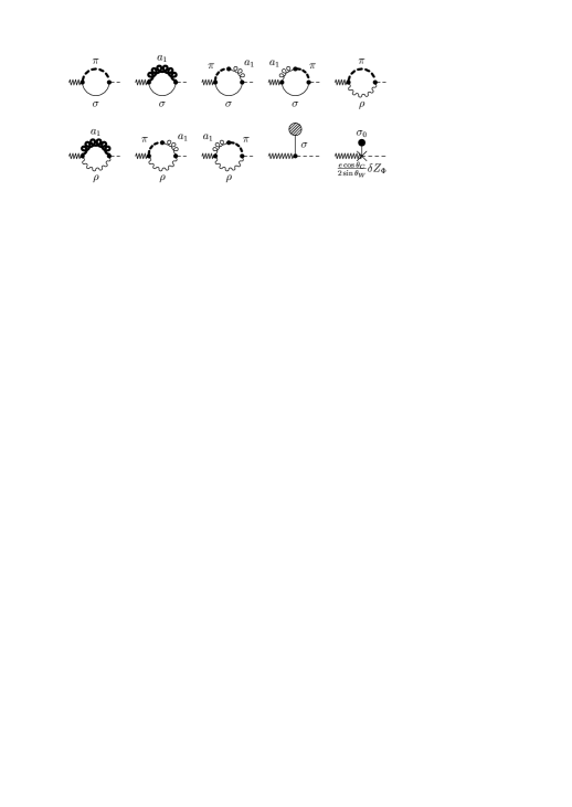
Figure 14: One-loop diagrams for the mixed $W-\pi$ self energy, $-i\Sigma_{W\pi}^{\mu}$ .

The last diagram is generated by the counterterm one obtains by performing the minimal substitution given by Eq. (44) in the wave-function renormalization counterterm, Eq. (59). The 1PI one-loop corrected $W-\pi$ vertex can now be written as

$$\big{(}\Gamma_{W\pi}(q)\big{)}_{ab}^{\mu}=-\delta_{ab}\Big{(}\frac{e\cos\theta_{C}}{2\sin\theta_{W}}\sigma_{0}\,q^{\mu}+i\Sigma_{W\pi}^{\mu}(q)\Big{)}=:-\frac{e\cos\theta_{C}}{2\sin\theta_{W}}q^{\mu}\delta_{ab}F_{W\pi}(q^{2})\,,$$ (79)

with $q$ being the incoming momentum of the $W$ boson. Then the full $W-\pi$ vertex reads

$$\big{(}\Gamma_{W\pi}^{\mathrm{tot}}(q)\big{)}_{ab}^{\mu} =-\frac{e\cos\theta_{C}}{2\sin\theta_{W}}q^{\mu}\delta_{ab}\Big{(}F_{W\pi}(q^{2})-\frac{F_{W{a_{1}}}^{l}(q^{2})F_{\pi{a_{1}}}(q^{2})}{m_{a_{1}}^{2}-\xi q^{2}-\Sigma_{{a_{1}}{a_{1}}}^{l}(q^{2})}\Big{)}$$

$$=:-\frac{e\cos\theta_{C}}{2\sin\theta_{W}}q^{\mu}\delta_{ab}F_{W\pi}^{\mathrm{tot}}(q^{2})\,.$$ (80)

The longitudinal $W$-boson self energy, which determines the spectral function $a_{0}(q^{2})$ according to Eqs. (69) and (71), is given by

$$\Sigma_{W}^{A\,l}(q^{2})=\Sigma_{WW}^{A\,l}(q^{2})+\Big{(}\frac{e\cos\theta_{C}}{2\sin\theta_{W}}\Big{)}^{2}\Big{(}\frac{\big{(}F_{W{a_{1}}}^{l}(q^{2})\big{)}^{2}}{m_{a_{1}}^{2}-\xi q^{2}-\Sigma_{{a_{1}}{a_{1}}}^{l}(q^{2})}+\frac{q^{2}\big{(}F_{W\pi}^{\mathrm{tot}}(q^{2})\big{)}^{2}}{q^{2}-m_{\pi\,{0}}^{2}-\Sigma_{\pi}(q^{2})}\Big{)}\,.$$ (81)

The full $W-\pi$ vertex can also be used to calculate the one-loop corrected pion decay constant,

$$f_{\pi}^{(1)}=F_{W\pi}^{\mathrm{tot}}(m_{\pi}^{(1)\,2})\;\sqrt{Z_{\pi}^{(1)}}\,,$$ (82)

with $m_{\pi}^{(1)}$ and $Z_{\pi}^{(1)}$ defined as

$$m_{\pi}^{(1)\,2}=m_{\pi\,{0}}^{2}+\Sigma_{\pi}(m_{\pi}^{(1)\,2})\,,$$ (83)

$$Z_{\pi}^{(1)}=\Big{(}1-\frac{d}{dq^{2}}\Sigma_{\pi}(q^{2})\Big{|}_{q^{2}=m_{\pi}^{(1)\,2}}\Big{)}^{-1}\,.$$ (84)

5 Results

5.1 Determination of model parameters

Our model has two groups of parameters, the bare parameters of the Lagrangian,

$$\mu^{2},\quad\lambda^{2},\quad c,\quad\xi,\quad m_{0}^{2}\,,\quad g,\quad h_{1}\,,\quad h_{2}\,,\quad f,$$

and the finite parts of the counterterms,

$$\overline{\delta Z}_{\Phi}\,,\quad\overline{\delta\mu^{2}},\quad\overline{\delta\lambda^{2}},\quad\overline{\delta Z}_{Y}\,,\quad\overline{\delta m_{0}^{2}}\,,\quad\overline{\delta g},\quad\overline{\delta h}_{1}\,,\quad\overline{\delta h}_{2}\,,\quad\overline{\delta f}\,.$$

However, not all of these parameters are independent of each other. Our final results do not separately depend on $f$ and $\overline{\delta f}$, but only on the combination $(f+\overline{\delta f})$, and the counterterms $\overline{\delta m_{0}^{2}}$ and $\overline{\delta h}_{2}$ always appear in the combination $(\overline{\delta m_{0}^{2}}+\overline{\delta h}_{2}\sigma_{0}^{2})$. Thus we have altogether 16 independent parameters.

In practice it is more convenient to employ Eqs. (17), (33), (35), (42), and (48) and to express the bare parameters $\mu^{2}$, $\lambda^{2}$, $c$, $g$, $h_{1}$ , and $h_{2}$ through the more physical quantities

$$m_{\pi}\,,\quad m_{\sigma}\,,\quad m_{\rho}\,,\quad m_{a_{1}}\,,\quad f_{\pi}\,,\quad\mathrm{and}\quad g_{\rho\pi\pi}^{\mathrm{eff}}\,.$$

For the parameter fixing one should keep in mind that our approximation is not self consistent. In particular, unstable particles calculated in one-loop approximation decay into tree-level particles. Hence one should not only fit the one-loop properties to the empirical values, but also the tree-level masses, in order to get the proper phenomenology. For instance, the decay ${a_{1}}\rightarrow\pi\pi\pi$ is modeled by the decay modes ${a_{1}}\rightarrow\pi\rho$ (dominant) and ${a_{1}}\rightarrow\pi\sigma$ (small), with stable $\rho$ and $\sigma$ mesons. As we shall see, for the $\pi\rho$ decay mode, this works rather well for invariant masses above $m_{\pi}+m_{\rho}$, if both, the pion and the $\rho$ meson, at tree level have already their physical masses, i.e. $m_{\pi}=m_{\pi}^{(1)}$ = 140 MeV and $m_{\rho}=m_{\rho}^{(1)}$. As a definition for the $\rho$-meson mass $m_{\rho}^{(1)}$ we choose the position where the $\rho$-meson spectral function has its maximum, $m_{\rho}^{(1)}=767\;\mathrm{MeV}$.

Besides the pion mass we also fit the pion decay constant to its empirical value, $f_{\pi}$ = 93 MeV. Again we demand that the tree-level value is equal to the corrected one, $f_{\pi}=f_{\pi}^{(1)}$. Among others, this will be important for later applications of the model at non-vanishing temperatures, where the effects will be dominated by thermally excited tree-level pions.

Similarly, we demand that $m_{a_{1}}$ and $m_{\sigma}$ at tree-level coincide with the corrected ${a_{1}}$- and $\sigma$-meson masses, i.e. $m_{a_{1}}^{(1)}=m_{a_{1}}$ and $m_{\sigma}^{(1)}=m_{\sigma}$. The corrected masses are again defined as the positions where the spectral functions have their maxima. As we will discuss below, one should not blindly fit the $a_{1}$-meson mass to any value given in the literature. Instead, we will use the ${a_{1}}$-meson mass to fit the peak position of the axial vector spectral function $a_{1}(q^{2})$. For the $\sigma$-meson, which is not a well established resonance, we will take two different values, namely 600 MeV and 800 MeV.

The width of the $\rho$ meson depends on two parameters, $g_{\rho\pi\pi}^{\mathrm{eff}}$ and $\overline{\delta Z}_{Y}$ . The latter has also influence on the ${a_{1}}$ meson width. Hence, both parameters can be fixed by fitting the widths of the vector and axial-vector spectral functions, $v_{1}(q^{2})$ and $a_{1}(q^{2})$.

The width of the vector spectral function $v_{1}(q^{2})$ being fixed, its height can be adjusted with the parameter $(f+\overline{\delta f})$. The height of the axial vector spectral function $a_{1}(q^{2})$ is then adjusted by changing $\overline{\delta g}$, which, in practice, is quite complicated, since this parameter changes also many other quantities because of $\pi-{a_{1}}$ mixing.

The parameter $\xi$ acts as a cutoff for the momenta of longitudinally polarized vector mesons. If we set arbitrarily $\xi=0.1$, the masses of the longitudinally polarized vector mesons are $\gtrsim 2\;\mathrm{GeV}$, which lies still in the range of hadronic scales, but is high enough to avoid unphysical thresholds in the energy range of interest. Since the masses of the longitudinally polarized vector mesons behave as $1/\sqrt{\xi}$, we can obtain reasonable fits also for smaller values of $\xi$, e.g. for $\xi=0.025$.

The remaining undetermined parameter is $m_{0}$, the vector-meson mass in the restored phase. This value is partially constrained by the upper limit of the ${a_{1}}\rightarrow\pi\sigma$ branching ratio. The relation between $m_{0}$ and the ${a_{1}}\pi\sigma$ vertex function $\Gamma_{{a_{1}}\pi\sigma}$ is the following. $\Gamma_{{a_{1}}\pi\sigma}$ has two contributions, corresponding to the diagrams (a) and (b) in Fig. 2, with the outgoing $\rho$-meson lines replaced by $\sigma$-meson lines. The sum of both terms yields

$$\big{(}\Gamma_{{a_{1}}\pi\sigma}^{\mathrm{(a+b)}}\big{)}^{\mu}_{ab}=-g\delta_{ab}\Big{(}\frac{m_{0}^{2}-\xi k^{2}}{m_{a_{1}}^{2}-\xi k^{2}}2k^{\mu}+q^{\mu}\Big{)}\,.$$ (85)

For transversely polarized ${a_{1}}$ mesons, the $q^{\mu}$ term does not contribute. Thus, for $\xi m_{\pi}^{2}\ll m_{a_{1}}^{2}$, the partial decay width ${a_{1}}\rightarrow\pi\sigma$ is proportional to $m_{0}^{4}$ . However, even for $m_{0}=0$ the axial-vector spectral function $a_{1}(q^{2})$ has small $\pi\sigma$ contributions from the direct $W-\pi-\sigma$ coupling (first four diagrams in Fig. 12).

It turns out that we can achieve reasonable fits for $m_{0}\lesssim 400\;\mathrm{MeV}$. Of course a particularly interesting case is $m_{0}=0$, which corresponds to a vanishing vector meson bare mass in the restored phase (“Brown-Rho scenario”). Therefore, in the following we will present fits with $m_{0}=0$ as well as with the maximum possible value $m_{0}=400\;\mathrm{MeV}$. Together with the two values for the $\sigma$-meson mass this leads to four different parameter sets, which are listed in Table 1. As explained in Sect. 3.1, the scale parameter $\Lambda$ can be chosen arbitrarily, since the dependence of the final results on $\Lambda$ can be absorbed in the finite parts of the counterterms. On the other hand, the numerical values of the finite parts of the counterterms are meaningful only if the value of $\Lambda$ is known, and this is the reason why it is listed in Table 1.

$$\begin{array}[]{|l|l|r|r|r|r|}\hline\cr&&\hfill\mbox{Fit A}\hfill&\hfill\mbox{Fit B}\hfill&\hfill\mbox{Fit C}\hfill&\hfill\mbox{Fit D}\hfill\\ \hline\cr\raisebox{0.0pt}[0.0pt][0.0pt]{\mbox{\parbox[t]{85.35826pt}{\raggedright Input\@add@raggedright}}}&m_{\pi}\,/\;\mathrm{MeV}&140&140&140&140\\ &m_{\sigma}\,/\;\mathrm{MeV}&600&600&800&800\\ &f_{\pi}\,/\;\mathrm{MeV}&93&93&93&93\\ &\xi&0.1&0.1&0.1&0.1\\ &m_{0}\,/\;\mathrm{MeV}&0&400&0&400\\ &\Lambda\,/\;\mathrm{MeV}&1000&1000&1000&1000\\ \hline\cr\raisebox{0.0pt}[0.0pt][0.0pt]{\mbox{\parbox[t]{85.35826pt}{\raggedright Obtained from fit of $v_{1}$ and $a_{1}$ and from conditions specified in the text of Sect.\@ \ref{Sectparamfit}\@add@raggedright}}}&m_{\rho}\,/\;\mathrm{MeV}&767&767&767&767\\ &m_{a_{1}}\,/\;\mathrm{MeV}&1064&1062&1056&1054\\ &g_{\rho\pi\pi}^{\mathrm{eff}}&7.63&7.77&7.92&7.97\\ &(f+\overline{\delta f})&0.076&0.078&0.083&0.084\\ &\overline{\delta Z}_{\Phi}&-9.36&-9.30&-8.48&-8.56\\ &\overline{\delta\mu^{2}}\,/\;\mathrm{MeV}^{2}&6666^{2}&3873^{2}&6211^{2}&3522^{2}\\ &\overline{\delta\lambda^{2}}&-3147&-1421&-2671&-1221\\ &\overline{\delta Z}_{Y}&0.260&0.064&0.069&-0.056\\ &(\overline{\delta m_{0}^{2}}+\overline{\delta h}_{2}\sigma_{0}^{2})\,/\;\mathrm{MeV}^{2}&2352^{2}&2197^{2}&2245^{2}&2128^{2}\\ &\overline{\delta h_{1}}&20.1&14.9&15.4&9.11\\ &\overline{\delta g}&33.7&32.5&29.3&29.0\\ \hline\cr\raisebox{0.0pt}[0.0pt][0.0pt]{\mbox{\parbox[t]{85.35826pt}{\raggedright Computed from parameters listed above\@add@raggedright}}}&\sigma_{0}\,/\;\mathrm{MeV}&150.9&152.5&153.7&154.1\\ &m_{\pi\,{0}}\,/\;\mathrm{MeV}&86.1&85.3&84.6&84.4\\ &\lambda^{2}&7.74&7.58&13.4&13.3\\ &c\,/\;\mathrm{MeV}^{3}&103.8^{3}&103.5^{3}&103.2&103.1\\ &g&5.55&5.52&5.47&5.45\\ &h_{1}&23.9&23.2&22.3&22.0\\ &h_{2}&25.8&18.4&24.9&18.0\\ &-i\overline{T}/m_{\sigma}^{2}\,/\;\mathrm{MeV}&9.80&14.40&7.65&10.82\\ \hline\cr\end{array}$$

Table 1: Model parameters and related quantities in four different fits.

5.2 The $\rho$ meson and the vector correlator

The real- and imaginary parts of the $\rho$-meson propagators $G_{\rho}(q^{2})=1/(q^{2}-m_{\rho}^{2}-\Sigma_{\rho}^{t}(q^{2}))$ obtained for parameter sets A and D of Table 1 are displayed in the left panel of Fig. 15. As a result of the fitting procedure described in the previous section the propagators look very similar for both sets. In fact, the curves for the two other parameter sets, B and C, lie in between.

Figure 15: Left panel: the Real- and imaginary part of the $\rho$-meson propagator as a function of $M=\sqrt{q^{2}}$ for the parameter sets A and D listed in Table 1. Right panel: the $\pi\pi$ scattering phase shifts in the $J=1,I=1$ channel for parameter set A (the three other parameter sets give the same result). The data are taken from Ref. [31].

In the right panel of Fig. 15 we show the $\pi\pi$ scattering phase shifts in the $J=1,I=1$ channel. Near the resonance, $s\approx m_{\rho}^{2}$, the $\pi\pi$ $T$-matrix in this channel is clearly dominated by the $s$-channel $\rho$-meson exchange. Thus the scattering phase shifts are given by $\tan\delta_{1}^{1}=\mathrm{Im}\,G_{\rho}/\mathrm{Re}\,G_{\rho}$. As can be seen in the figure, the phase shifts obtained in this way fit the data up to $1\;\mathrm{GeV}$. In this region the four parameter sets of Table 1 lead to practically identical results.

The electromagnetic form factor of the pion is not simply proportional to the $\rho$-meson propagator as in Sakurai’s vector dominance model, in which the photon can couple to the two pions only via the $\rho$ meson. Instead, we have to consider also the direct coupling of the photon to two pions. Thus the pion electromagnetic form factor is given by

$$F_{\pi}(q^{2})=1+\frac{q^{2}F_{\gamma\rho}(q^{2})g_{\rho\pi\pi}^{\mathrm{eff}}}{q^{2}-m_{\rho}^{2}-\Sigma_{\rho}^{t}(q^{2})}\,.$$ (86)

The result can be seen in the left panel of Fig. 16, together with the experimental data.

Figure 16: Left panel: the electromagnetic form factor of the pion for the parameter sets A and D listed in Table 1. The curves for the parameter sets B and C lie in between. The data are taken from Refs. [32, 33]. Right panel: the spectral function $v_{1}(q^{2})$, together with data obtained from $\tau$ decay by the ALEPH collaboration [22].

Except for the small structure at $q^{2}=0.61\;\mathrm{GeV}^{2}$ caused by $\rho-\omega$ mixing, the data are well reproduced up to $q^{2}\approx 1.5\;\mathrm{GeV}^{2}$ (fit D) or even higher (fit A).

In the right panel of Fig. 16 we display our results for the vector-isovector spectral function $v_{1}(q^{2})$. In the resonance region, the experimental data are perfectly reproduced, but in the continuum region, above $q^{2}\approx 1\;\mathrm{GeV}^{2}$, we get only a small fraction of the strength measured by the ALEPH collaboration. This is obviously related to the fact that above $1\;\mathrm{GeV}$ four-pion channels become important. In our model, these are partially contained as $\pi{a_{1}}$, $\sigma\rho$ and $\rho\rho$ channels. The threshold for the $\sigma\rho$ channel at $q^{2}=1.87\;\mathrm{GeV}^{2}$ for fit A and $q^{2}=2.46\;\mathrm{GeV}^{2}$ for fit D is clearly visible, and also the $\rho\rho$ channel gives a sizable contribution above $2.35\;\mathrm{GeV}^{2}$, whereas the $\pi{a_{1}}$ channel contributes almost nothing. At first sight this is surprising, since in the $\rho$-meson spectral function the $\pi{a_{1}}$ channel is relatively strong (in the left panel of Fig. 15 one can see the threshold as a small kink at $1.2\;\mathrm{GeV}$). However, in the vector spectral function two amplitudes interfere destructively, namely $(\gamma\rightarrow\pi{a_{1}})$ and $(\gamma\rightarrow\rho\rightarrow\pi{a_{1}})$. This interference is absent in the $\sigma\rho$ and $\rho\rho$ channels, because the $\sigma\rho$ channel can be reached only via the $\rho$ meson $(\gamma\rightarrow\rho\rightarrow\sigma\rho)$, while for the $\rho\rho$ channel only the direct coupling exists $(\gamma\rightarrow\rho\rho)$.

5.3 The ${a_{1}}$ meson and the axial-vector correlator

Before the precise $\tau$ decay measurements by the ALEPH collaboration [22], the knowledge about the axial vector correlator and the properties of the $a_{1}$ meson was more or less uncertain, and even in the latest particle data book [24], mass and width of the $a_{1}$ meson still have large uncertainties: $m_{a_{1}}=1230\pm 40\;\mathrm{MeV}$ and $\Gamma_{a_{1}}=250$ to $600\;\mathrm{MeV}$. However, as pointed out in Ref. [30], the discrepancy of different experiments to some extent stems from the use of different parametrizations of the ${a_{1}}$ propagator in the analyses. Therefore, one must be careful when taking over parameters from another model. We have decided to fit the axial-vector spectral function ourselves and not to restrict the parameters to the values listed in the particle data book.

The resulting ${a_{1}}$ propagator $G_{a_{1}}(q^{2})=1/(q^{2}-m_{a_{1}}^{2}-\Sigma_{a_{1}}^{t}(q^{2}))$ is shown in the left panel of Fig. 17.

Figure 17: Left panel: the real- and imaginary part of the ${a_{1}}$ propagator as a function of $M=\sqrt{q^{2}}$ for the parameter sets A and D listed in Table 1. The curves for the parameter sets B and C lie in between. Right panel: the transverse axial-vector spectral function $a_{1}$ as a function of $q^{2}$. The data are taken from Ref. [22].

The mass, defined as the position of the maximum of $-\mathrm{Im}\,G_{a_{1}}$, is rather low (see Table 1). However, if we adopt another usual convention, defining the mass as the position of the zero of $\mathrm{Re}\,G_{a_{1}}$, we obtain higher values between $m_{a_{1}}=1136\;\mathrm{MeV}$ (fit D) and $m_{a_{1}}=1159\;\mathrm{MeV}$ (fit A). The ${a_{1}}$ meson width is defined as the difference of the two masses where $-\mathrm{Im}\,G_{a_{1}}$ crosses one half of its maximum. We find $\Gamma_{a_{1}}=424\;\mathrm{MeV}$ for fit A and $\Gamma_{a_{1}}=393\;\mathrm{MeV}$ for fit D.

The spectral function of the transverse axial-vector correlator, $a_{1}(q^{2})$, is displayed in the right panel of Fig. 17. Between $0.9$ and $2\;\mathrm{GeV}^{2}$ we can fit the ALEPH data very well. In this range the spectral function is almost saturated by three-pion states [22], which in our model are approximated by $\pi\rho$ states with sharp $\rho$ mesons. Over a wide range of $q^{2}$ this seems to be adequate. Only in the region $q^{2}\lesssim(m_{\pi}+m_{\rho})^{2}$, of course, some strength is missed. Above $2\;\mathrm{GeV}^{2}$ the spectral function receives sizeable contributions from five-pion states [22]. These are partially contained in our model as $\sigma{a_{1}}$ and $\rho{a_{1}}$ states (for fit A, the $\sigma{a_{1}}$ threshold is visible at $2.77\;\mathrm{GeV}^{2}$), but this is obviously not sufficient in order to fit the data.

In Fig. 18 it is shown that up to the $\tau$ mass the exclusive three-pion final state can very well be approximated by a $\pi\rho$ final state with a sharp $\rho$ meson.

Figure 18: Left panel: the three-pion invariant mass distribution of $\tau^{-}\rightarrow\pi^{-}\pi^{-}\pi^{+}\nu_{\tau}$ for the parameter sets A and D listed in Table 1. Right panel: the invariant mass distributions of $\pi^{-}\pi^{-}$ (theoretical curves and crosses) and $\pi^{+}\pi^{-}$ pairs (dots) of $\tau^{-}\rightarrow\pi^{-}\pi^{-}\pi^{+}\nu_{\tau}$ . The data are taken from Refs. [21] and [34].

In the left panel we display the three-pion invariant mass distribution measured by the ARGUS collaboration [21] and obtained in our model as the sum of $1/2$ of the $\pi\rho$ and $2/3$ of the $\pi\sigma$ spectrum (see App. A). The $\pi\sigma$ channel contributes only between $1.3\,\%$ (fit C) and $5.4\,\%$ (fit B) to the integrated spectrum, which lies below the upper limit of $6\,\%$ given in Ref. [21].

In the right panel of Fig. 18 we display the $\pi^{-}\pi^{-}$ and $\pi^{+}\pi^{-}$ invariant mass distributions of the decay $\tau^{-}\rightarrow\pi^{-}\pi^{-}\pi^{+}\nu_{\tau}$. The experimental data show that the $\pi^{+}\pi^{-}$ distribution (dots) is the sum of the $\pi^{-}\pi^{-}$ distribution (crosses) and a distribution which is concentrated around the $\rho$-meson mass, indicating that the $\pi^{-}\pi^{-}\pi^{+}$ final state is indeed reached via a $\pi^{-}\rho^{0}$ intermediate state. The interference term, which is responsible for the fact that at low invariant masses the $\pi^{+}\pi^{-}$ distribution lies below the $\pi^{-}\pi^{-}$ distribution, is small. The $\pi^{-}\pi^{-}$ distribution which corresponds to our model (see App. B) is in good agreement with the data. Since we do not take into account the $\rho$-meson width and the interference term, the corresponding $\pi^{+}\pi^{-}$ distribution would be given by the $\pi^{-}\pi^{-}$ distribution plus a delta function at the $\rho$-meson mass (and a small delta function at the $\sigma$-meson mass).

5.4 The longitudinal axial-vector correlator

As one can see from Eqs. (81) to (84) the longitudinal axial-vector correlator has a pole at $q^{2}=m_{\pi}^{(1)\,2}\ (=m_{\pi}^{2})$ with residue $4\pi^{2}f_{\pi}^{(1)\,2}\ (=4\pi^{2}f_{\pi}^{2})$, i.e.

$$a_{0}(q^{2})=4\pi^{2}f_{\pi}^{2}\delta(q^{2}-m_{\pi}^{2})+\tilde{a}_{0}(q^{2})\,,$$ (87)

where $\tilde{a}_{0}(q^{2})$ denotes the contribution of multi-particle channels. According to Eq. (81), the longitudinal $W$-boson self energy consists of three terms. The corresponding contributions to $\tilde{a}_{0}(q^{2})$ are shown in Fig. 19.

Figure 19: The multi-particle contribution of the longitudinal axial-vector spectral function, $\tilde{a}_{0}(q^{2})$, calculated with the parameters from fit A in Table 1. For the meaning of the different terms see Eq. (81).

The first term gives a positive contribution to $\tilde{a}_{0}(q^{2})$, whereas the other terms contain interferences of several amplitudes and are negative. The sum of the three terms is of course positive, but almost zero. In fact, it is not visible in the figure since it is about a factor $10^{-4}$ smaller than the first contribution. To be more quantitative, we integrate the strength of $\tilde{a}_{0}(q^{2})$ up to $m_{\tau}=1777\;\mathrm{MeV}$. With the parameters of fit A we find $\int_{0}^{m_{\tau}^{2}}dq^{2}\,\tilde{a}_{0}(q^{2})=75\;\mathrm{MeV}^{2}$, which has to be compared with the strength $4\pi^{2}f_{\pi}^{2}=0.34\;\mathrm{GeV}^{2}$ of the single-pion contribution.

The smallness of $\tilde{a}_{0}(q^{2})$ is a manifestation of the PCAC hypothesis. Usually the PCAC hypothesis is formulated as $\partial^{\mu}\vec{j}_{\mu}^{5}=f_{\pi}m_{\pi}^{2}\vec{\pi}$ . However, beyond tree level this is almost meaningless, since the field operator $\pi_{a}$ has non-vanishing matrix elements $\langle f|\pi_{a}|0\rangle$ not only for single-pion states $|f\rangle$, but also for multi-particle states, e.g. in our model for $\pi\sigma$, $\pi\rho$, ${a_{1}}\sigma$ and ${a_{1}}\rho$ states. In fact, as pointed out by Weinberg [35], the PCAC assumption should be interpreted in a different way, namely that $\tilde{a}_{0}(q^{2})$, which is directly related to the multi-particle content of $\partial^{\mu}j_{\mu\,a}^{5}|0\rangle$, is negligible. Obviously this is fulfilled very well in our model.

5.5 The $\sigma$-meson propagator

A general problem of models with linearly realized chiral symmetry is that at tree level it predicts the existence of a sharp scalar isoscalar meson, which has not been found experimentally. However, in the latest particle data book [24] a meson with these quantum numbers is listed as “$f_{0}(400-1200)$ or $\sigma$”. This particle has a very large width (approximately as large as the mass) due to the decay into two pions. Since our calculation contains the $\sigma\rightarrow\pi\pi$ graph, one could expect that it should be possible to get a satisfactory description of the $\sigma$ meson. Unfortunately, this is not the case for the following reasons:

The $\sigma\pi\pi$ vertex has four contributions, analogous to the four contributions to the $\rho\pi\pi$ vertex of the gauged linear $\sigma$ model shown in Fig. 1. These amplitudes interfere destructively. If the outgoing pions are on the mass shell, the total vertex function has a zero at some value of the invariant mass $M$ of the $\sigma$ meson. For the parameter sets A and B listed in Table 1, this zero lies at $754\;\mathrm{MeV}$ and $705\;\mathrm{MeV}$, respectively. This is above the tree-level $\sigma$ mass, $m_{\sigma}=600\;\mathrm{MeV}$, but the amplitude is already very small for $M\approx m_{\sigma}$. The authors of Ref. [19] hoped that this effect could improve the description of the $\sigma$ meson, since they believed that the width obtained from the linear $\sigma$ model without vector mesons was too large. However, now the width is much too small, as can be seen in the left panel of Fig. 20, where we display the $\sigma$-meson propagator for the parameter sets A and B. The different normalization results from the fact that we adjust the wave-function renormalization constant $\overline{\delta Z}_{\Phi}$ for the pion propagator and not for the $\sigma$-meson propagator.

Another problem arises from the fact that, at the two-pion threshold, the $\sigma$-meson self energy usually becomes strongly attractive (i.e. negative). Since the $\sigma\pi\pi$ vertex function at low $q^{2}$ is dominated by the ordinary $\sigma$ model vertex $\propto\lambda^{2}\sigma_{0}$, with $\lambda^{2}\propto m_{\sigma}^{2}-m_{\pi\,{0}}^{2}$, this effect is stronger for higher $\sigma$-meson masses and has therefore more dramatic consequences for the parameter sets C and D. For parameter set C we find a two-pion bound state at $M=231\;\mathrm{MeV}$, while for parameter set D the $\sigma$-meson propagator has the wrong sign at low $M$ and a pole in the complex plane. For illustration, we have plotted the inverse $\sigma$-meson propagator in the right panel of Fig. 20.

Figure 20: Left panel: the real- and imaginary part of the $\sigma$-meson propagator for parameter sets A and B. Right panel: the real- and imaginary parts of the inverse $\sigma$-meson propagator for parameter sets C and D.

Obviously the $\sigma$-meson cannot be described in one-loop approximation. A good description of the $\sigma$-meson in the linear $\sigma$ model can be obtained by summing the $\pi\pi$ loops in the self energy to all orders (RPA) in the large-$N$ limit ($N$ = number of pions) [36]. Summing the $\pi\pi$ loops reduces the strong attraction in the real part at the two-pion threshold. However, the application of the RPA to our Lagrangian would be extremely difficult. On the other hand, for the vector mesons, in which we are interested, the one-loop calculation seems to be sufficient.

6 Conclusions

We have presented a chirally symmetric hadronic model for the vector and axial-vector correlators in vacuum. The starting point was the linear $\sigma$ model extended by $\rho$-meson and $a_{1}$ fields in a chirally symmetric way. Unlike the gauged linear $\sigma$ model, which leads to phenomenological difficulties (see Sect. 2.1), our Lagrangian is only symmetric under global, but not under local $SU(2)_{L}\times SU(2)_{R}$ transformations. After all, chiral symmetry is also only an (approximate) global symmetry in QCD.

For a realistic description of $\rho$ and $a_{1}$ we could not stay at tree-level, where all mesons are stable particles. In order to include the most important decay channels, $\rho\rightarrow\pi\pi$ and $a_{1}\rightarrow\rho\pi$, we performed a one-loop calculation. Here care had to be exercised, not to destroy the symmetries of the model by choosing an unsuited regularization scheme. We have decided to use dimensional regularization in order to isolate the divergences, which are then subtracted by chirally symmetric counterterms.

The price to pay for giving up the requirement of a local chiral symmetry is the loss of the so-called current-field identity which directly relates the vector and axial-vector currents to the meson fields. Therefore some additional work was needed to construct the correlators in a consistent way.

In the last part of the paper we have presented numerical results. We have fixed our parameters to reproduce the empirical values of $m_{\pi}$ and $f_{\pi}$ and the peak regions of the vector and axial vector spectral functions, which have been extracted by the ALEPH collaboration from the $\tau$ decay. Basically, this leaves two parameters undetermined, namely the mass of the $\sigma$-meson, which is not a well established resonance in nature, and the mass parameter $m_{0}$. The latter is the fraction of the bare $\rho$-meson mass which is not proportional to the vacuum expectation value of the $\sigma$ field, i.e. the fraction which would survive in the restored phase. From our fit we only found an upper limit of $400\;\mathrm{MeV}$ for $m_{0}$. On the other hand, a particularly interesting case is $m_{0}=0$, which corresponds to a vanishing bare vector meson mass in the restored phase (“Brown-Rho scenario”). Therefore, we have performed calculations with $m_{0}=0$ and with $m_{0}=400\;\mathrm{MeV}$, both for two different $\sigma$-meson masses, $m_{\sigma}=600\;\mathrm{MeV}$ and $m_{\sigma}=800\;\mathrm{MeV}$.

All fits describe the peak regions of the experimental spectral functions equally well and also give a satisfactory description of the pion electromagnetic form factor, the $\pi\pi$ phase shifts in the vector-isovector channel, and the $\pi^{-}\pi^{-}\pi^{+}$ and $\pi^{-}\pi^{-}$ mass distributions for the decay $\tau^{-}\rightarrow\pi^{-}\pi^{-}\pi^{+}\nu_{\tau}$ . At higher energies, $q^{2}\geq 1\;\mathrm{GeV}^{2}$ in the vector channel and $q^{2}\geq 2\;\mathrm{GeV}^{2}$ in the transverse axial-vector channel our fits underestimate the empirical spectral functions. In these regions four-pion (vector channel) or five-pion (axial-vector channel) final states become relevant, which are not properly contained in our one-loop calculation.

The longitudinal axial correlator is completely dominated by the pion pole, in agreement with the PCAC hypothesis. The remaining strength, which is due to the small explicit breaking of chiral symmetry in our Lagrangian, is the result of a delicate cancellation of three terms which are four orders of magnitude larger than their sum. This nicely demonstrates the consistency of our model with chiral symmetry as well as the stability of the numerics.

In the present paper we have restricted ourselves to vacuum properties. However, having the technology developed, it is now straightforward to calculate the correlators at finite temperatures. Work in this direction is in progress. The extension to finite baryon density in a chirally symmetric way is obviously more difficult.

Acknowledgements

One of us (M. U.) acknowledges support from the Studienstiftung des deutschen Volkes. This work was supported in part by the BMBF.

Appendix A The three-pion invariant mass distribution of $\tau^{-}\rightarrow\pi^{-}\pi^{-}\pi^{+}\nu_{\tau}$

The differential $\tau$ decay width has the form

$$\frac{d\Gamma_{\tau\rightarrow\pi^{-}\pi^{-}\pi^{+}\nu_{\tau}}}{dM_{3\pi}}=G_{F}^{2}\cos^{2}{\theta_{C}}\frac{(m_{\tau}^{2}-M_{3\pi}^{2})^{2}}{2\pi^{2}m_{\tau}^{3}M_{3\pi}}\big{(}m_{\tau}^{2}H_{\pi^{-}\pi^{-}\pi^{+}}^{l}+(m_{\tau}^{2}+2M_{3\pi}^{2})H_{\pi^{-}\pi^{-}\pi^{+}}^{t}\big{)}\,.$$ (88)

In this formula, $G_{F}=e^{2}/(4\sqrt{2}\sin^{2}\theta_{W}m_{W}^{2})$ denotes Fermi’s coupling constant and $H_{\pi^{-}\pi^{-}\pi^{+}}^{l}$ and $H_{\pi^{-}\pi^{-}\pi^{+}}^{t}$ are the longitudinal and transverse components of the so-called hadron tensor, respectively. Under the assumption of PCAC, the longitudinal component can be neglected.

In our model the $\pi^{-}\pi^{-}\pi^{+}$ spectrum consists of $1/2$ of the $\pi\rho$ plus $2/3$ of the $\pi\sigma$ spectrum, i.e.

$$H_{\pi^{-}\pi^{-}\pi^{+}}^{t}(M_{3\pi}^{2})=\frac{1}{2}H_{\pi\rho}^{t}(M_{3\pi}^{2})+\frac{2}{3}H_{\pi\sigma}^{t}(M_{3\pi}^{2})\,.$$ (89)

The $\pi\rho$ and $\pi\sigma$ hadron tensors are given by

$$H_{\pi\rho}^{t}(q^{2})= \frac{1}{3}\Big{(}\frac{q_{\mu}q_{\mu^{\prime}}}{q^{2}}-g_{\mu\mu^{\prime}}\Big{)}\int\frac{d^{3}{k_{\pi}}}{(2\pi)^{3}}\,\frac{1}{2k_{\pi}^{0}}\int\frac{d^{3}{k_{\rho}}}{(2\pi)^{3}}\,\frac{1}{2k_{\rho}^{0}}(2\pi)^{4}\delta(q-k_{\pi}-k_{\rho})$$

$$\times Z_{\pi\,{1}}\Big{(}\frac{k_{\rho\,\nu}k_{\rho\,\nu^{\prime}}}{m_{\rho}^{2}}-g_{\nu\nu^{\prime}}\Big{)}\big{(}A_{W\pi\rho}\big{)}_{1bc}^{\mu\nu}\big{(}A_{W\pi\rho}^{*}\big{)}_{1bc}^{\mu^{\prime}\nu^{\prime}}\,,$$ (90)

$$H_{\pi\sigma}^{t}(q^{2})= \frac{1}{3}\Big{(}\frac{q_{\mu}q_{\mu^{\prime}}}{q^{2}}-g_{\mu\mu^{\prime}}\Big{)}\int\frac{d^{3}{k_{\pi}}}{(2\pi)^{3}}\,\frac{1}{2k_{\pi}^{0}}\int\frac{d^{3}{k_{\sigma}}}{(2\pi)^{3}}\,\frac{1}{2k_{\sigma}^{0}}(2\pi)^{4}\delta(q-k_{\pi}-k_{\sigma})$$

$$\times Z_{\pi\,{1}}\big{(}A_{W\pi\sigma}\big{)}_{1b}^{\mu}\big{(}A_{W\pi\sigma}^{*}\big{)}_{1b}^{\mu^{\prime}}\,,$$ (91)

with $k_{\pi}^{0}=\sqrt{m_{\pi}^{2}+\vec{k}_{\pi}^{2}}$ , $k_{\rho}^{0}=\sqrt{m_{\rho}^{2}+\vec{k}_{\rho}^{2}}$ , $k_{\sigma}^{0}=\sqrt{m_{\sigma}^{2}+\vec{k}_{\sigma}^{2}}$ and

$$\big{(}A_{W\pi\rho}\big{)}_{abc}^{\mu\nu}= \frac{\sin\theta_{W}}{e\cos{\theta_{C}}}\Big{(}\big{(}\Gamma_{W\pi\rho}\big{)}_{abc}^{\mu\nu}+\big{(}\Gamma_{W{a_{1}}}\big{)}_{ad}^{\mu\kappa}i\big{(}G_{a_{1}}(q^{2})\big{)}_{\kappa\lambda}\big{(}\Gamma_{{a_{1}}\pi\rho}\big{)}_{dbc}^{\lambda\nu}\Big{)}\,,$$ (92)

$$\big{(}A_{W\pi\sigma}\big{)}_{ab}^{\mu}= \frac{\sin\theta_{W}}{e\cos{\theta_{C}}}\Big{(}\big{(}\Gamma_{W\pi\sigma}\big{)}_{ab}^{\mu}+\big{(}\Gamma_{W{a_{1}}}\big{)}_{ad}^{\mu\kappa}i\big{(}G_{a_{1}}(q^{2})\big{)}_{\kappa\lambda}\big{(}\Gamma_{{a_{1}}\pi\sigma}\big{)}_{db}^{\lambda}\Big{)}\,.$$ (93)

The vertex functions $\Gamma_{W\pi\rho}$ and $\Gamma_{W\pi\sigma}$ are defined analogously to Fig. 2.

The curves shown in the left panel of Fig. 18 are normalized as follows:

$$\frac{dN_{\pi^{-}\pi^{-}\pi^{+}}}{dM_{3\pi}}=N_{\tau^{-}}\tau_{\tau^{-}}\frac{d\Gamma_{\tau^{-}\rightarrow\pi^{-}\pi^{-}\pi^{+}\nu_{\tau}}}{dM_{3\pi}}=\frac{N_{\pi^{-}\pi^{-}\pi^{+}}\tau_{\tau^{-}}}{B(\tau^{-}\rightarrow\pi^{-}\pi^{-}\pi^{+}\nu_{\tau})}\,\frac{d\Gamma_{\tau^{-}\rightarrow\pi^{-}\pi^{-}\pi^{+}\nu_{\tau}}}{dM_{3\pi}}\,,$$ (94)

where $N_{\pi^{-}\pi^{-}\pi^{+}}=37170$ is the total number of $\pi^{-}\pi^{-}\pi^{+}$ events [21], $\tau_{\tau^{-}}=290.0\,\mathrm{fs}$ is the $\tau$ lifetime [22], and $B(\tau^{-}\rightarrow\pi^{-}\pi^{-}\pi^{+}\nu_{\tau})=9.15\,\%$ is the branching ratio [22].

Appendix B The $\pi^{-}\pi^{-}$ invariant mass distribution of $\tau^{-}\rightarrow\pi^{-}\pi^{-}\pi^{+}\nu_{\tau}$

Since our model does not contain the $\pi^{-}\pi^{-}\pi^{+}$ final state, but only $\pi^{-}\rho^{0}$ and $\pi^{-}\sigma$ final states, the $\pi^{-}\pi^{-}$ distribution cannot be computed directly. Instead we must interprete the $\rho^{0}$ or $\sigma$ meson in the final state, with momentum $k_{\rho}$ or $k_{\sigma}$ , respectively, as a $\pi^{+}\pi^{-}$ pair with momenta $p_{\pi^{+}}$ and $p_{\pi^{-}}$ (i.e. $p_{\pi^{+}}+p_{\pi^{-}}=k_{\rho}$ or $k_{\sigma}$ , respectively). For simplicity let us first look at the $\pi\sigma$ final state.

In the rest frame of the $\sigma$ meson the kinematics is given by

$$k_{\sigma} =(m_{\sigma},\vec{0})\,,$$

$$k_{\pi^{-}} =(q_{0}-m_{\sigma},\vec{q})\,,\quad q_{0}=\frac{q^{2}-m_{\sigma}^{2}-m_{\pi}^{2}}{2m_{\sigma}}\,,\quad|\vec{q}|=\frac{\sqrt{(q^{2}-m_{\pi}^{2}-m_{\sigma}^{2})^{2}-4m_{\pi}^{2}m_{\sigma}^{2}}}{2m_{\sigma}}\,,$$

$$p_{\pi^{\pm}} =\Big{(}\frac{m_{\sigma}}{2},\mp\vec{p}\Big{)}\,,\quad|\vec{p}|=\sqrt{\frac{m_{\sigma}^{2}}{4}-m_{\pi}^{2}}\,,\quad\vec{p}\cdot\vec{q}=|\vec{p}||\vec{q}|z\,.$$ (95)

Thus the $\pi^{-}\pi^{-}$ invariant mass depends only on $q^{2}$ and $z=\cos(\vec{p},\vec{q})$:

$$M_{2\pi}^{2}=\frac{q^{2}-m_{\sigma}^{2}+3m_{\pi}^{2}}{2}-2|\vec{p}||\vec{q}|z\,.$$ (96)

Let $P_{\sigma}(z)$ be the probability for a certain angle between $\vec{p}$ and $\vec{q}$. Since the $\sigma$ meson decays into a $\pi^{+}\pi^{-}$ pair in $s$ wave, the angular distribution in its rest frame is isotropic, i.e. $P_{\sigma}(z)=\mbox{const.}=1/2$. Now the $\pi\sigma$ contribution to the $\pi^{-}\pi^{-}$ invariant mass spectrum can be written as

$$\frac{dN_{\pi^{-}\pi^{-}}}{dM_{2\pi}^{2}} =\int_{9m_{\pi}^{2}}^{\infty}\!\!dq^{2}\,\Big{(}\frac{dN_{\pi^{-}\pi^{-}\pi^{+}}^{(\pi\sigma)}}{dM_{3\pi}^{2}}\Big{)}_{M_{3\pi}^{2}=q^{2}}$$

$$\phantom{=\int_{9m_{\pi}^{2}}^{\infty}\!\!dq^{2}\,}\times\int_{-1}^{1}\!\!dz\,P_{\sigma}(z)\delta\big{(}M_{2\pi}^{2}-(q^{2}-m_{\sigma}^{2}+3m_{\pi}^{2})/2+2|\vec{p}||\vec{q}|z\big{)}$$

$$=\int_{q^{2}_{-}}^{q^{2}_{+}}\!\!dq^{2}\,\Big{(}\frac{dN_{\pi^{-}\pi^{-}\pi^{+}}^{(\pi\sigma)}}{dM_{3\pi}^{2}}\Big{)}_{M_{3\pi}^{2}=q^{2}}\,\,\frac{1}{2|\vec{p}||\vec{q}|}P_{\sigma}\big{(}(q^{2}-m_{\sigma}^{2}+3m_{\pi}^{2}-2M_{2\pi}^{2})/(4|\vec{p}||\vec{q}|)\big{)}\,,$$ (97)

where $dN_{\pi^{-}\pi^{-}\pi^{+}}^{(\pi\sigma)}/dM_{3\pi}$ is the $\pi\sigma$ contribution to the three-pion spectrum discussed in App. A, and the integration boundaries $q^{2}_{\pm}$ in the last line are given by

$$q^{2}_{\pm}=\frac{2m_{\pi}^{4}+m_{\sigma}^{2}M_{2\pi}^{2}\pm 2|\vec{p}|m_{\sigma}M_{2\pi}\sqrt{M_{2\pi}^{2}-4m_{\pi}^{2}}}{2m_{\pi}^{2}}\,.$$ (98)

For the $\pi\rho$ contribution the situation is very similar if one replaces everywhere $m_{\sigma}$ by $m_{\rho}$. The only complication comes from the fact that the angular distribution cannot be assumed to be isotropic, since the $\rho$ meson decays into a $\pi^{+}\pi^{-}$ pair in $p$ wave. In order to obtain the angular distribution, we assume that the $\rho$ meson is measured by a fictitious detector, which forces it onto its mass shell without changing its spin, and the decay into two pions takes place after this measurement. Under these conditions the angular distribution is given by the square of the amplitude

$$B^{\mu}\varepsilon_{abc}=(A_{W\pi\rho})^{\mu\nu}_{abc}(p_{\pi^{-}\,\nu}-p_{\pi^{+}\,\nu})\,,$$ (99)

averaged over the three transverse $W$ polarizations, and evaluated for the kinematics given above (but with $m_{\sigma}$ replaced by $m_{\rho}$):

$$P_{\rho}(z)\propto\Big{(}\frac{q_{\mu}q_{\mu^{\prime}}}{q^{2}}-g_{\mu\mu^{\prime}}\Big{)}B^{\mu}B^{*\,\mu^{\prime}}=c_{0}+c_{2}z^{2}\,.$$ (100)

The normalized angular distribution is then given by

$$P_{\rho}(z)=\frac{c_{0}+c_{2}z^{2}}{2(c_{0}+c_{2}/3)}\,.$$ (101)

References

- [1] J.J. Sakurai, Ann. Phys. 11 (1960) 1.
-
[2]
G. Agakichiev et al., CERES collaboration,
Phys. Rev. Lett. 75 (1995) 1272;
P. Wurm for the CERES collaboration, Nucl. Phys. A 590 (1995) 103c. - [3] G.Q. Li, C.M. Ko and G.E. Brown, Phys. Rev. Lett. 75 (1995) 4007.
- [4] G.E. Brown and M. Rho, Phys. Rev. Lett. 66, (1991) 2720.
- [5] B. Friman and H.J. Pirner, Nucl.Phys. A 617 (1997) 496.
- [6] W. Peters, M. Post, H. Lenske, S. Leupold and U. Mosel, Nucl. Phys. 632 (1998) 109.
- [7] G. Chanfray and P. Schuck, Nucl. Phys. A 555 (1993) 329.
- [8] M. Herrmann, B. Friman and W. Nörenberg, Nucl. Phys. A 560 (1993) 411.
- [9] G. Chanfray, R. Rapp and J. Wambach, Phys. Rev. Lett. 76 (1996) 368.
- [10] R. Rapp and J. Wambach, Adv. Nucl. Phys. 25 (2000) 1.
-
[11]
M. Dey, V.L. Eletsky and B.L. Ioffe,
Phys. Lett. B 252 (1990) 620;
V.L. Eletsky and B.L. Ioffe, Phys. Rev. D 51 (1995) 2371. -
[12]
G. Chanfray, J. Delorme and M. Ericson,
Nucl. Phys. A 637 (1998) 421;
G. Chanfray, J. Delorme, M. Ericson and M. Rosa-Clot, nucl-th/9809007. - [13] B. Krippa, Phys. Lett. B 427 (1998) 13.
- [14] M. Gell-Mann and M. Lévy, Nuovo Cimento 16 (1960) 705.
- [15] B.W. Lee and H.T. Nieh, Phys. Rev. 166 (1968) 1507.
- [16] G.’t Hooft, Nucl. Phys. B 35 (1971) 167.
- [17] U.-G. Meißner, Phys. Rep. 161 (1988) 213.
- [18] S. Gasiorowicz and D.A. Geffen, Rev. Mod. Phys. 41 (1969) 531.
- [19] P. Ko and S. Rudaz, Phys. Rev. D 50 (1994) 6877.
- [20] R.D. Pisarski, hep-ph/9505257; Phys. Rev. D 52 (1995) R3773.
- [21] H. Albrecht et al. (ARGUS Collaboration), Z. Phys. C 58 (1993) 61.
- [22] R. Barate et al. (ALEPH Collaboration), Eur. Phys. J. C 4 (1998) 409.
- [23] C. Itzykson and J.-B. Zuber, Quantum Field Theory, McGraw-Hill (New York) 1980.
- [24] D.E. Groom et al. (Particle Data Group), Eur. Phys. J. C 15 (2000) 1.
- [25] N.M. Kroll, T.D. Lee and B. Zumino, Phys. Rev. 157 (1967) 1376.
- [26] Z. Aouissat, G. Chanfray, P. Schuck and J. Wambach, Nucl. Phys. A 603 (1996) 458.
- [27] H. van Hees, doctoral thesis, Darmstadt 2000.
- [28] L.R. Ram Mohan, Phys. Rev. D 14 (1976) 2670.
- [29] B.W. Lee, Nucl. Phys. B 9 (1969) 649.
- [30] N. Isgur, C. Morningstar and C. Reader, Phys. Rev. D 39 (1989) 1357.
- [31] C.D. Froggatt and J.L. Petersen, Nucl. Phys. B 129 (1977) 89.
- [32] S.R. Amendolia et al., Phys. Lett. B 138 (1984) 454; Phys. Lett. B 146 (1984) 116.
- [33] L.M. Barkov et al., Nucl. Phys. B 256 (1985) 365.
- [34] A. Walther, doctoral thesis, Dortmund 1991.
- [35] S. Weinberg, The Quantum Theory of Fields, Vol. II: Modern Applications, Cambridge University Press 1996.
- [36] Z. Aouissat, P. Schuck and J. Wambach, Nucl. Phys. A 618 (1997) 402.