BNL-HET-01/6, hep-ph/0102241 — 19 February 2001
Soft and virtual corrections to $pp\to H+X$ at next-to-next-to-leading order

Abstract

1 Introduction

In the past two decades the predictions of the standard model have been confirmed with remarkable precision. Still, the agent of electroweak symmetry breaking remains elusive. The simplest mechanism introduces a single complex scalar doublet. Three components of the doublet give mass to the $W$ and $Z$ bosons, leaving a single neutral particle, the Higgs boson, as the signature of the symmetry breaking sector. This scenario is called the minimal standard model (SM) and forms the benchmark for the investigation of electroweak symmetry breaking.

In their final run, the experiments at the CERN $e^{+}e^{-}$ collider LEP established a lower mass limit for a SM Higgs boson of $\sim 113$ GeV [1]. This value severely challenges the reach of the Fermilab Tevatron. Nonetheless, there are indications that the Higgs boson is not much heavier than this limit. Fits to precision electroweak data actually prefer a value of the Higgs boson mass that is well below the exclusion limit and place a $95\%$ confidence level upper limit near $200$ GeV [2]. Supersymmetric extensions to the SM, which have at least two Higgs doublets and therefore at least five observable Higgs bosons, prefer that the mass of the lightest Higgs be below approximately $135$ GeV [3]. Detailed studies indicate that, with sufficient luminosity, the Tevatron could be sensitive to Higgs bosons somewhat beyond the $W^{+}W^{-}$ threshold [4].

At hadron colliders, the dominant production mechanism for Higgs bosons of mass below $\sim 700$ GeV is gluon fusion. The Tevatron however will only be able to make limited use of this production channel. For Higgs boson masses well above the $W^{+}W^{-}$ threshold, the production rate is too small to be observed. For masses well below the $W^{+}W^{-}$ threshold, the dominant $b\bar{b}$ decay mode is overwhelmed by QCD background, and the production rate is insufficient to allow observation of rare decay modes like $H\to\gamma\gamma$. Thus except for a window around the $W^{+}W^{-}$ threshold where that decay mode may be observable, the Tevatron Higgs search will rely on associated production with a $W$ or $Z$ boson rather than gluon fusion [5].

At the CERN Large Hadron Collider (LHC) the gluon fusion production mechanism will be extremely important. For lighter Higgs boson masses, the $b\bar{b}$ decay mode will still be overwhelmed by QCD effects, but because of the high machine luminosity and the large gluon luminosity at relatively small parton energy fractions, the LHC will be able to measure the $H\to\gamma\gamma$ decay mode. This will be important not only as a discovery channel (if the Higgs boson has not yet been found) but also as a means of studying Higgs properties like its coupling to top quarks.

Unfortunately, the gluon fusion process is currently not fully under control. The next-to-leading order (NLO) corrections to the production rate were computed ten years ago and were found to be extremely large, of order $70-100\%$ [6, 7]. Such large corrections clearly ask for the evaluation of higher order terms in the perturbative series in order to arrive at a solid theoretical understanding of the process. In this paper, we present the soft plus virtual corrections to inclusive Higgs production at next-to-next-to-leading order (NNLO). For the relevant values of $M_{H}\sim 100$–$200$ GeV and the center-of-mass (c.m.s.) energies at Tevatron (2 GeV) and LHC (14 TeV), these terms are not expected to dominate the full result. Nevertheless, they represent a first step towards the complete answer, in the sense that they comprise a well-defined, ultraviolet and infrared finite, gauge and renormalization group invariant piece. By comparing to existing estimates on the NNLO corrections for $gg\to H$, we conclude that the evaluation of the full answer is necessary.

2 Higgs production through light parton scattering

2.1 Leading order

Assuming the standard model as the theory of particle interactions, the coupling of the Higgs boson to gluons is mediated by a quark loop. In the following we will neglect all quark masses except for the top mass. In this case only the top quark contributes, because the Yukawa couplings are proportional to the fermion masses. The lowest order diagram is then shown in Fig. 1 (a). It was computed some time ago [8] and leads to the cross section

$$\begin{split}\sigma_{\rm LO}(gg\to H)&={G_{\rm F}\alpha_{s}^{2}(\mu^{2})\over 128\sqrt{2}\pi}\tau^{2}\delta(1-x)\left|1+(1-\tau)f(\tau)\right|^{2}\,,\\ f(\tau)&=\left\{\begin{array}[]{ll}\arcsin^{2}{1\over\sqrt{\tau}}\,,&\tau\geq 1,\\ -{1\over 4}\left[\ln{1+\sqrt{1-\tau}\over 1-\sqrt{1-\tau}}-i\pi\right]^{2}\,,&\tau<1,\end{array}\right.\\ \tau&=4M_{t}^{2}/M_{H}^{2}\,,\qquad x=M_{H}^{2}/s\,,\end{split}$$ (1)

where $s$ is the partonic center-of-mass energy, $G_{\rm F}$ the Fermi coupling constant, $\alpha_{s}$ the strong coupling constant (which depends on the renormalization scale $\mu$), $M_{t}$ the pole mass of the top quark, and $M_{H}$ the Higgs boson mass.

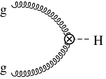
(a)	(b)

Figure 1: Leading order diagram to the process $gg\to H$: (a) in full QCD; (b) in the effective theory [Eq. (2)]. The straight solid lines represent the top quark, the symbol $\otimes$ denotes the effective vertex.

2.2 Effective Lagrangian

The lowest threshold of the diagram in Fig. 1 (a) is at $M_{H}=2M_{t}$. This means that an expansion in terms of $M_{H}/M_{t}$ is expected to converge for $M_{H}<2M_{t}$. In fact, it has been shown that the NLO K-factor for this process is excellently approximated up to much larger Higgs boson masses, even by keeping only the first term of such an expansion. With a top mass of around $M_{t}=175$ GeV and the experimental data favoring a relatively low Higgs boson mass between 100 to 200 GeV, we feel that keeping only the leading term in $M_{H}/M_{t}$ is also well justified at NNLO.

We therefore integrate out the top quark and compute amplitudes using QCD with five active flavors and the following effective Lagrangian [9] for the Higgs-gluon interaction:

$$\begin{split}{\cal L}_{\rm eff}&=-{H\over 4v}C_{1}\,{\cal O}_{1}=-{H\over 4v}C_{1}^{\rm B}\,{\cal O}_{1}^{\rm B},\qquad\qquad{\cal O}_{1}=G^{a}_{\mu\nu}G^{a\,\mu\nu}\,,\end{split}$$ (2)

where $G^{a}_{\mu\nu}$ is the gluon field strength tensor. In the approximation that all light flavors are massless, this effective Lagrangian is renormalization group invariant, but the coefficient function $C_{1}^{\rm B}$ and the operator ${\cal O}_{1}^{\rm B}$ must each be renormalized. Below, we give the renormalized value of $C_{1}$ while the renormalization of ${\cal O}_{1}^{\rm B}$ and its matrix elements is discussed in Sect. 3.1.

The coefficient function contains the residual logarithmic dependence on the top quark mass and has been computed up to ${\cal O}(\alpha_{s}^{4})$ [10]. For our purposes, we need it only up to ${\cal O}(\alpha_{s}^{3})$ [10, 11]. The coefficient function in the modified minimal subtraction scheme ($\overline{\mbox{\small MS}}$) is

$$\begin{split}C_{1}&=-{1\over 3}{\alpha_{s}\over\pi}\bigg{\{}1+{11\over 4}{\alpha_{s}\over\pi}+\left({\alpha_{s}\over\pi}\right)^{2}\left[{2777\over 288}+{19\over 16}l_{t}+n_{f}\left(-{67\over 96}+{1\over 3}l_{t}\right)\right]+\ldots\bigg{\}}\,,\end{split}$$ (3)

where $l_{t}=\ln(\mu^{2}/M_{t}^{2})$ and $M_{t}$ is the on-shell top quark mass. $\alpha_{s}\equiv\alpha_{s}^{(5)}(\mu^{2})$ is the $\overline{\mbox{\small MS}}$ renormalized QCD coupling constant for five active flavors, and $n_{f}$ is the number of massless flavors. In our numerical results, we always set $n_{f}=5$.

Using the effective Lagrangian of Eq. (2), the lowest order amplitude for the process $gg\to H$ reduces from the one-loop diagram in Fig. 1 (a) to the tree-level diagram in Fig. 1 (b).

2.3 Sub-Processes: virtual, single real, double real

For a complete treatment of the process $pp\to H$ in NNLO QCD one needs to compute the partonic processes which must then be convoluted with parton distribution functions.

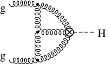
(a)	(b)	(c)

Figure 2: Sample two-loop diagrams contributing to the virtual corrections at NNLO.

(a)	(b)	(c)

Figure 3: Typical diagrams contributing to (a) single and (b) double real radiation of gluons and (c) double real radiation of quark-antiquark pairs at NNLO. The dashed line is the Higgs boson and “$\otimes$” denotes the effective Higgs-gluon vertex.

The partonic subprocesses are:

1. Virtual corrections to two loops:
   $gg\to H$.

2. Single real radiation to one loop:
   $gg\to Hg$ , $q\bar{q}\to Hg$ , $qg\to Hq$ , $\bar{q}g\to H\bar{q}$.

3. Double real radiation at the tree level:
   $gg\to Hgg$ , $gg\to Hq\bar{q}$ , $q\bar{q}\to Hgg$ , $q\bar{q}\to Hq\bar{q}$ , $qg\to Hqg$ , $\bar{q}g\to H\bar{q}g$.

2.4 The soft approximation

Radiative corrections to inclusive production fall into three categories: delta function terms $\propto\delta(1-x)$, large logarithms of the form $\ln^{n}(1-x)/(1-x)$, and hard scattering terms that have at most a logarithmic singularity as $x\to 1$, where $x$ is the ratio of the Higgs boson mass squared to the incoming parton c.m.s. energy squared [see Eq. (1)]. In the kinematically similar Drell-Yan process [12] and in inclusive Higgs production at NLO [6], it has been observed that the delta function and large log terms are important though not necessarily dominant parts of the radiative corrections.

Virtual corrections add only delta function contributions while real emission corrections contribute to all three categories. The soft approximation is obtained by taking the limit $x\to 1$. In doing so, one is left with only those terms that scale like $(1-x)^{-1-a\epsilon}$, where $\epsilon=(4-d)/2$, and $d$ is the number of space-time dimensions assumed for the regularization of divergent integrals. The term $(1-x)^{-1-a\epsilon}$ must be interpreted as a distribution,

$$\begin{split}f_{a\epsilon}(x)&\equiv-a\epsilon\,(1-x)^{-1-a\epsilon}=\delta(1-x)+\sum_{n=0}^{\infty}{(-a\epsilon)^{n+1}\over n!}{\cal D}_{n}(x)\,,\end{split}$$ (4)

where ${\cal D}_{n}(x)$ is a “plus” distribution,

$$\begin{split}{\cal D}_{n}(x)&=\left[{\ln^{n}(1-x)\over 1-x}\right]_{+},\\ \int_{0}^{1}\!dx\,h(x){\cal D}_{n}(x)&=\int_{0}^{1}\!dx\left[h(x)-h(1)\right]{\ln^{n}(1-x)\over 1-x}.\end{split}$$ (5)

Thus, towers of the large logarithm terms ${\cal D}_{n}(x)$ can be trivially obtained from knowledge of the $\delta(1-x)$ terms.

3 Results

3.1 Renormalization of matrix elements

We write the partonic cross section as follows:

$$\begin{split}\sigma&={\pi\over 64v^{2}}C_{1}^{2}(\alpha_{s})Z^{2}_{1}(\alpha_{s}){1\over(1-\epsilon)^{2}}\left[\rho_{A}+\rho_{B}+\rho_{C}\right]\,.\end{split}$$ (6)

$\rho_{A}$ is the contribution from virtual corrections, while $\rho_{B}$ and $\rho_{C}$ represent the contributions from single and double real emission, respectively. $Z_{1}(\alpha_{s})$ is the global renormalization factor for the composite operator in the effective Lagrangian [13]:

$$\begin{split}{\cal O}_{1}&=Z_{1}(\alpha_{s}){\cal O}_{1}^{\rm B}\,,\\ \mbox{with}\quad Z_{1}(\alpha_{s})&={1\over 1-\beta(\alpha_{s})/\epsilon}=1-{\alpha_{s}\over\pi}\,{\beta_{0}\over\epsilon}+\left({\alpha_{s}\over\pi}\right)^{2}\,\left[{\beta_{0}^{2}\over\epsilon^{2}}-{\beta_{1}\over\epsilon}\right]+{\cal O}(\alpha_{s}^{3})\,.\end{split}$$ (7)

Here, $\beta(\alpha_{s})$ is the QCD beta function:

$$\begin{split}\beta(\alpha_{s})&=-{\alpha_{s}\over\pi}\beta_{0}-\left({\alpha_{s}\over\pi}\right)^{2}\beta_{1}+{\cal O}(\alpha_{s}^{3})\,,\\ \beta_{0}&={1\over 4}\left(11-{2\over 3}n_{f}\right)\,,\qquad\beta_{1}={1\over 16}\left(102-{38\over 3}n_{f}\right)\,.\end{split}$$ (8)

In the following sections, we will list the results for $\rho_{A}$, $\rho_{B}$, and $\rho_{C}$ in terms of the bare coupling $\alpha_{s}^{\rm B}$ which is related to the $\overline{\mbox{\small MS}}$ renormalized coupling by

$$\begin{split}\alpha_{s}^{\rm B}&={\cal N}^{-1}Z_{\alpha}(\alpha_{s})\,\alpha_{s}\,,\\ \mbox{where}\qquad{\cal N}&\equiv\exp[\epsilon(-\gamma_{\rm E}+\ln 4\pi)]\,,\end{split}$$ (9)

and $\gamma_{\rm E}=0.577216\ldots$ is the Euler constant. The charge renormalization constant $Z_{\alpha}(\alpha_{s})$ is

$$\begin{split}Z_{\alpha}(\alpha_{s})&=1-{\alpha_{s}\over\pi}\,{\beta_{0}\over\epsilon}+\left({\alpha_{s}\over\pi}\right)^{2}\,\left({\beta_{0}^{2}\over\epsilon^{2}}-{\beta_{1}\over 2\epsilon}\right)+{\cal O}(\alpha_{s}^{3})\,.\end{split}$$ (10)

3.2 Two-loop virtual corrections

The two-loop virtual corrections have been calculated in [14]. Typical diagrams are shown in Fig. 2. Since gluons are massless, these diagrams depend on only a single scale $q^{2}=M_{H}^{2}$, where $q$ is the momentum of the Higgs boson. They were calculated using the method of ref. [15] which allows one to relate the integration-by-parts identities for the two-loop three-point functions of Fig. 2 to those for three-loop two-point functions [16]. The coding of the integration routines was done in FORM [17] and was based on the program MINCER [18]. It is worth mentioning that the resulting program is capable of dealing with much more general diagrams than the ones considered for this calculation. In particular it solves integrals with (in principle) arbitrary integer powers of the propagators. This may become useful in future applications where expansions have to be applied to the diagrams.

The expression for $\rho_{A}$ is given in ref. [14]:

$$\begin{split}\rho_{A}&=\rho_{A}^{(0)}+{\alpha_{s}^{\rm B}\over\pi}\,\rho_{A}^{(1)}+\left({\alpha_{s}^{\rm B}\over\pi}\right)^{2}\,\rho_{A}^{(2)}+{\cal O}(\alpha_{s}^{3})\,,\end{split}$$ (11)

$$\begin{split}\rho_{A}^{(0)}(x)&=(1-\epsilon)\,\delta(1-x)\,,\\ \rho_{A}^{(1)}(x)&={\cal N}\left({\mu^{2}\over M_{H}^{2}}\right)^{\epsilon}\,\delta(1-x)\,\left[-{3\over\epsilon^{2}}+{3\over\epsilon}+{21\over 2}\zeta_{2}+\epsilon\left(-3-{21\over 2}\zeta_{2}+7\zeta_{3}\right)\right]\,,\\ \rho_{A}^{(2)}(x)&={\cal N}^{2}\left({\mu^{2}\over M_{H}^{2}}\right)^{2\epsilon}\,\delta(1-x)\,\bigg{\{}{9\over 2\epsilon^{4}}+{1\over\epsilon^{3}}\left(-{105\over 16}+{1\over 8}n_{f}\right)\\ &\quad+{1\over\epsilon^{2}}\left(-{17\over 8}-{243\over 8}\zeta_{2}+{1\over 12}n_{f}\right)\\ &\quad+{1\over\epsilon}\bigg{[}{553\over 48}+{981\over 16}\zeta_{2}-{159\over 8}\zeta_{3}+n_{f}\left(-{53\over 72}-{15\over 8}\zeta_{2}\right)\bigg{]}\\ &\quad+{6749\over 144}+{255\over 8}\zeta_{2}+{85\over 4}\zeta_{3}+{1161\over 20}\zeta_{2}^{2}+n_{f}\left(-{137\over 27}-{5\over 4}\zeta_{2}-{7\over 4}\zeta_{3}\right)\bigg{\}}\,,\end{split}$$ (12)

where $\zeta_{n}\equiv\zeta(n)$ is Riemann’s $\zeta$ function which takes the particular values

$$\begin{split}\zeta_{2}&=\pi^{2}/6=1.64493\ldots\\ \zeta_{3}&=1.20206\ldots.\end{split}$$ (13)

3.3 Single real radiation

The one-loop amplitudes for the processes ($ii$) in Sect. 2.3 were computed in ref. [19] in the form of helicity amplitudes to order $\epsilon^{0}$. Unfortunately, these amplitudes are not sufficient for our purpose. The integration over two-particle phase space generates infrared singularities which take the form of single and double poles in $\epsilon$ which combine with the ${\cal O}(\epsilon)$ and ${\cal O}(\epsilon^{2})$ pieces of the amplitude to produce finite contributions to the cross section. If we were to work in the four dimensional helicity scheme [20], where gluons have two polarization states, helicity amplitudes extended to higher order in $\epsilon$ would suffice. However, since we work in the conventional dimensional regularization scheme, gluons have $d-2=2-2\epsilon$ polarizations. Thus, in addition to helicity amplitudes we also need amplitudes corresponding to the extra “$\epsilon$” polarizations. Both the additional pieces of the amplitudes and the integration over the two-particle phase space have been evaluated and will be presented elsewhere [21]. That calculation includes the full dependence on the center-of-mass energy. Here we are interested in the soft limit, to which we find that only the $gg\to Hg$ process contributes. The result is

$$\begin{split}\rho_{B}&={\alpha_{s}^{\rm B}\over\pi}\,\rho_{B}^{(1)}+\left({\alpha_{s}^{\rm B}\over\pi}\right)^{2}\,\rho_{B}^{(2)}+{\cal O}(\alpha_{s}^{3})\,,\\ \end{split}$$ (14)

$$\begin{split}\rho_{B}^{(1)}(x)&={\cal N}\left({\mu^{2}\over M_{H}^{2}}\right)^{\epsilon}f_{2\epsilon}(x)\,\left[{3\over\epsilon^{2}}-{3\over\epsilon}-{9\over 2}\zeta_{2}+\epsilon\left({9\over 2}\zeta_{2}-7\zeta_{3}\right)\right]\,,\\ \rho_{B}^{(2)}(x)&={\cal N}^{2}\left({\mu^{2}\over M_{H}^{2}}\right)^{2\epsilon}\bigg{\{}f_{2\epsilon}(x)\,\bigg{[}-{9\over\epsilon^{4}}+{9\over\epsilon^{3}}+{45\over\epsilon^{2}}\,\zeta_{2}\\ &\quad\quad+{1\over\epsilon}\left(-9-45\,\zeta_{2}+42\,\zeta_{3}\right)-18-42\,\zeta_{3}-{603\over 10}\,\zeta_{2}^{2}\bigg{]}\\ &\quad+f_{4\epsilon}(x)\left[-{9\over 8\epsilon^{4}}+{9\over 8\epsilon^{3}}+{63\over 8\epsilon^{2}}\,\zeta_{2}+{1\over\epsilon}\left(-{63\over 8}\,\zeta_{2}+21\,\zeta_{3}\right)-21\,\zeta_{3}+{189\over 80}\,\zeta_{2}^{2}\right]\bigg{\}}\,.\end{split}$$ (15)

Expanding $f_{a\epsilon}(x)$ (see Eq. (4)), Eq. (15) describes both delta function and large logarithm contributions to the radiative corrections.

3.4 Double real radiation

The tree-level amplitudes for the processes ($iii$) of Sect. 2.3 with two partons in the final state was evaluated in [22], though again only as helicity amplitudes to ${\cal O}(\epsilon^{0})$. We have evaluated the full $\epsilon$ dependence in the conventional dimensional regularization scheme by computing all of the Feynman diagrams, squaring the amplitude and integrating over phase space, dropping terms that do not contribute in the soft limit as described in Sect. 2.4. We find that only the $gg\to Hgg$ and $gg\to Hq\bar{q}$ processes contribute with the result

$$\begin{split}\rho_{C}(x)&={\cal N}^{2}\left({\alpha_{s}^{\rm B}\over\pi}\right)^{2}\left({\mu^{2}\over M_{H}^{2}}\right)^{2\epsilon}f_{4\epsilon}(x)\bigg{\{}{45\over 8\epsilon^{4}}-{57\over 16\epsilon^{3}}+{1\over\epsilon^{2}}\left({17\over 8}-{81\over 2}\zeta_{2}\right)\\ &\quad+{1\over\epsilon}\left({203\over 48}+{417\over 16}\zeta_{2}-{975\over 8}\zeta_{3}\right)+{76\over 9}-{119\over 8}\zeta_{2}+{317\over 4}\zeta_{3}-{333\over 80}\zeta_{2}^{2}\\ &\quad+n_{f}\bigg{[}-{1\over 8\epsilon^{3}}-{1\over 12\epsilon^{2}}+{1\over\epsilon}\left(-{13\over 72}+{7\over 8}\zeta_{2}\right)-{10\over 27}+{7\over 12}\zeta_{2}+{31\over 12}\zeta_{3}\bigg{]}\bigg{\}}+{\cal O}(\alpha_{s}^{3})\,.\end{split}$$ (16)

The terms proportional to $n_{f}$ come from the $gg\to Hq\bar{q}$ sub-process. (See Fig. 3.)

3.5 Mass factorization

After combining all processes and renormalizing, there are still infrared singularities left over. These are all associated with mass factorization and can be absorbed into process independent functions $\Gamma_{ij}(x)$ associated with the incoming partons. The (IR-finite) partonic cross section, $\hat{\sigma}$, is defined implicitly by the relation

$$\begin{split}\sigma_{ij}&=\sum_{\bar{\imath},\bar{\jmath}}\hat{\sigma}_{\bar{\imath}\bar{\jmath}}\otimes\Gamma_{\bar{\imath}{i}}\otimes\Gamma_{\bar{\jmath}{j}},\end{split}$$ (17)

where $\sigma$ is defined in Eq. (6). The symbol $\otimes$ indicates convolution over longitudinal momentum fractions,

$$\begin{split}\left(f\otimes g\right)(x)&=\int_{0}^{1}dy\int_{0}^{1}dz\,f(y)\,g(z)\,\delta(x-yz),\end{split}$$ (18)

and the subscripts $\bar{\imath}$, $i$, etc., indicate parton identities. The $\Gamma_{ij}(x)$’s are given by

$$\begin{split}\Gamma_{ij}(x)&=\delta_{ij}\delta(1-x)-{\alpha_{s}\over\pi}{P^{(0)}_{ij}(x)\over\epsilon}\\ &\quad+\left({\alpha_{s}\over\pi}\right)^{2}\left[{1\over 2\epsilon^{2}}\left(\left(P^{(0)}_{ik}\otimes P^{(0)}_{kj}\right)(x)+\beta_{0}P^{(0)}_{ij}(x)\right)-{1\over 2\epsilon}P^{(1)}_{ij}(x)\right]+{\cal O}(\alpha_{s}^{3}),\end{split}$$ (19)

where the $P_{ij}^{(n)}$ are the $n$th order splitting functions [23, 24]. In the soft limit, only $P^{(n)}_{ij}$ with $i=j=g$ contribute. They are given by

$$\begin{split}P^{(0)}_{gg}(x)\,{\buildrel\rm soft\over{\longrightarrow}}\,\ &\left({11\over 4}-{n_{f}\over 6}\right)\delta(1-x)+3\,{\cal D}_{0}(x)\,,\\ P^{(1)}_{gg}(x)\,{\buildrel\rm soft\over{\longrightarrow}}\,\ &\left(6+{27\over 4}\zeta_{3}-{2\over 3}n_{f}\right)\,\delta(1-x)+\left({67\over 4}-{9\over 2}\,\zeta_{2}-{5\over 6}\,n_{f}\right)\,{\cal D}_{0}(x)\,.\end{split}$$ (20)

Writing

$$\begin{split}\sigma_{gg}=\sigma_{gg}^{(0)}+{\alpha_{s}\over\pi}\sigma_{gg}^{(1)}+\left({\alpha_{s}\over\pi}\right)^{2}\sigma_{gg}^{(2)}+\ldots\,,\end{split}$$ (21)

and similarly for $\hat{\sigma}_{gg}$, Eq. (17) can be solved for $\hat{\sigma}_{gg}$ order by order to give

$$\begin{split}\hat{\sigma}_{gg}^{(0)}(x)&=\sigma_{gg}^{(0)}(x)\equiv\sigma_{0}\,\delta(1-x)\,,\\ \hat{\sigma}_{gg}^{(1)}(x)&=\sigma_{gg}^{(1)}(x)+2\,\sigma_{0}\,P^{(0)}_{gg}(x)\,{1\over\epsilon}\,,\\ \hat{\sigma}_{gg}^{(2)}(x)&=\sigma_{gg}^{(2)}(x)-{1\over\epsilon^{2}}\sigma_{0}\left(\beta_{0}\,P^{(0)}_{gg}(x)+2\,(P_{gg}^{(0)}\otimes P_{gg}^{(0)})(x)\right)\\ &\quad\quad+{1\over\epsilon}\left(\sigma_{0}P_{gg}^{(1)}(x)+2\,(P_{gg}^{(0)}\otimes\hat{\sigma}_{gg}^{(1)})(x)\right)\,,\end{split}$$ (22)

where

$$\begin{split}\sigma_{0}\equiv{\pi\over 576v^{2}}\,\left({\alpha_{s}\over\pi}\right)^{2}\,(1+\epsilon+\epsilon^{2})\,.\end{split}$$ (23)

The convolutions in Eq. (22) can be evaluated with the help of the following relations

$$\begin{split}({\cal D}_{0}\otimes{\cal D}_{0})(x)\,{\buildrel\rm soft\over{\longrightarrow}}\,&\ -\zeta_{2}\,\delta(1-x)+2\,{\cal D}_{1}(x)\,,\\ ({\cal D}_{0}\otimes{\cal D}_{1})(x)\,{\buildrel\rm soft\over{\longrightarrow}}\,&\ \zeta_{3}\,\delta(1-x)-\zeta_{2}\,{\cal D}_{0}(x)+{3\over 2}{\cal D}_{2}(x)\,,\\ ({\cal D}_{0}\otimes{\cal D}_{2})(x)\,{\buildrel\rm soft\over{\longrightarrow}}\,&\ -{4\over 5}\,\zeta_{2}^{2}\,\delta(1-x)+2\,\zeta_{3}\,{\cal D}_{0}(x)-2\,\zeta_{2}\,{\cal D}_{1}(x)+{4\over 3}{\cal D}_{3}(x)\,,\\ ({\cal D}_{1}\otimes{\cal D}_{1})(x)\,{\buildrel\rm soft\over{\longrightarrow}}\,&\ -{1\over 10}\zeta_{2}^{2}\,\delta(1-x)-2\zeta_{2}{\cal D}_{1}(x)+{\cal D}_{3}(x)\,.\end{split}$$ (24)

3.6 Partonic cross section

Putting things together, we finally arrive at

$$\begin{split}\hat{\sigma}^{(0)}_{gg}&={\pi\over 576v^{2}}\,\left({\alpha_{s}\over\pi}\right)^{2}\delta(1-x)\,,\\ \hat{\sigma}^{(1),{\rm soft}}_{gg}&={\pi\over 576v^{2}}\left({\alpha_{s}\over\pi}\right)^{2}\left\{\delta(1-x)\left[{11\over 2}+6\,\zeta_{2}\right]-6\,{\cal D}_{0}(x)\,l_{H}+12\,{\cal D}_{1}(x)\right\}\,,\\ \hat{\sigma}^{(2),{\rm soft}}_{gg}&={\pi\over 576v^{2}}\left({\alpha_{s}\over\pi}\right)^{2}\bigg{\{}\delta(1-x)\left[{11399\over 144}+{133\over 2}\zeta_{2}-{165\over 4}\zeta_{3}-{9\over 20}\zeta_{2}^{2}\right.\\ &\quad\mbox{}+\left({27\over 2}+{33\over 2}\zeta_{2}-{171\over 2}\zeta_{3}\right)l_{H}-18\zeta_{2}\,l_{H}^{2}+{19\over 8}l_{t}\\ &\quad\mbox{}+n_{f}\left(-{1189\over 144}-{5\over 3}\zeta_{2}+{5\over 6}\zeta_{3}+\left(-{11\over 6}-\zeta_{2}\right)l_{H}+{2\over 3}l_{t}\right)\bigg{]}\\ &+{\cal D}_{0}(x)\bigg{[}-{101\over 3}+33\,\zeta_{2}+{351\over 2}\zeta_{3}+\left(-{133\over 2}+45\zeta_{2}\right)l_{H}-{33\over 4}l_{H}^{2}\\ &\quad+\mbox{}n_{f}\left({14\over 9}-2\,\zeta_{2}+{5\over 3}l_{H}+{1\over 2}l_{H}^{2}\right)\bigg{]}\\ &+{\cal D}_{1}(x)\left[133-90\,\zeta_{2}+33\,l_{H}+36\,l_{H}^{2}+n_{f}\left(-{10\over 3}-2\,l_{H}\right)\right]\\ &+{\cal D}_{2}(x)\left[-33-108\,l_{H}+2n_{f}\right]+72\,{\cal D}_{3}(x)\bigg{\}}\,,\end{split}$$ (25)

with $l_{H}\equiv\ln(\mu^{2}/M_{H}^{2})$ and $l_{t}\equiv\ln(\mu^{2}/M_{t})$. As a numerical example, let us set $\mu^{2}=M_{H}^{2}$ and insert the values $M_{H}=130$ GeV, $M_{t}=175$ GeV, and $\alpha_{s}=0.112$:

$$\begin{split}\hat{\sigma}_{gg}={\pi\over 576v^{2}}\left({\alpha_{s}\over\pi}\right)^{2}&\bigg{\{}[1+0.548+0.107]\,\delta(1-x)+[0+0+0.283]\,{\cal D}_{0}(x)\\ &+[0+0.428-0.040]\,{\cal D}_{1}(x)+[0+0-0.029]\,{\cal D}_{2}(x)\\ &+[0+0+0.092]\,{\cal D}_{3}(x)\bigg{\}}+{\cal O}(\alpha_{s}^{5})\,,\end{split}$$ (26)

where the individual numbers in square brackets correspond to the $\hat{\sigma}_{gg}^{(0)}$, $\hat{\sigma}_{gg}^{(1)}$, and $\hat{\sigma}_{gg}^{(2)}$ contributions. We observe that the coefficient of the $\delta$ function exhibits satisfactory convergence behavior. The magnitude of its NNLO contribution agrees roughly with the estimate of ref. [14].

3.6.1 Checks on the result

There are several checks that can be performed on our result. The first check is to observe that all poles in $\epsilon$ cancel to give us a finite result for $\hat{\sigma}^{(2),{\rm soft}}_{gg}$. Since the ${\cal D}_{n}(x)$ terms at order $\epsilon^{0}$ are linked to the poles of the real emission contributions, this already gives us great confidence in these terms. Below we will discuss an even more stringent constraint on the ${\cal D}_{n}$ coefficients.

Another check is to compare the three leading poles of the virtual two-loop corrections to the general result of ref. [25], where they are expressed in terms of universal functions that depend only on the identity of the external partons. The poles of the diagrammatic result of [14] fully obey this observation [26].

One can now combine the universal (three leading) NNLO pole terms with the NLO results $\rho_{A}^{(0,1)}$ and $\rho_{B}^{(1)}$ to derive the coefficients of ${\cal D}_{n}(x)$ for $n=1,2,3$ in $\hat{\sigma}_{gg}^{(2),\rm soft}$. Note that this uses only one-loop results and the universal behavior of QCD amplitudes and is done without reference to any of the newly calculated NNLO terms (including those of [14]). The pole structure of the real radiation terms must take the form

$$\begin{split}\left(\rho_{B}^{(2)}+\rho_{C}^{(2)}\right)_{\rm pole}&=f_{2\epsilon}(x)\left({\mu^{2}\over M_{H}^{2}}\right)^{2\epsilon}\left[{a_{24}\over\epsilon^{4}}+{a_{23}\over\epsilon^{3}}+{a_{22}\over\epsilon^{2}}+{a_{21}\over\epsilon}\right]\\ &\quad+f_{4\epsilon}(x)\left({\mu^{2}\over M_{H}^{2}}\right)^{2\epsilon}\left[{a_{44}\over\epsilon^{4}}+{a_{43}\over\epsilon^{3}}+{a_{42}\over\epsilon^{2}}+{a_{41}\over\epsilon}\right]\,.\end{split}$$ (27)

Expanding the $f_{n\epsilon}(x)$ terms as in Eq. (4) and requiring that all poles vanish from $\hat{\sigma}^{(2)}_{gg}$, we can solve for $a_{n4}$, $a_{n3}$ and $a_{n2}$ ($n=2,4$), while $a_{21}$ and $a_{41}$ remain undetermined. This solution is sufficient to fix the coefficients of ${\cal D}_{1}(x)$, ${\cal D}_{2}(x)$ and ${\cal D}_{3}(x)$ in $\hat{\sigma}^{(2)}_{gg}$, though not the coefficient of ${\cal D}_{0}(x)$. We find complete agreement between the ${\cal D}_{\{3,2,1\}}$ terms determined in this way and those found in Eq. (25).

Let us note that the absence of terms $\propto f_{n\epsilon}$ with $n\neq 2,4$ in Eq. (27) can be understood from the following consideration. The index $n$ of the $f_{n\epsilon}$ terms has two sources: the phase space elements for single and double real radiation contribute factors of $(1-x)^{1-2\epsilon}$ and $(1-x)^{3-4\epsilon}$ respectively (see e.g. Appendix E of ref. [12]), while the one-loop corrections to single real radiation amplitudes squared can contribute factors of $(1-x)^{m}$, $(1-x)^{m-\epsilon}$ or $(1-x)^{m-2\epsilon}$, where $m$ is an integer [19, 21]. [Tree-level amplitudes squared contain only integer powers of $(1-x)$.] The $(1-x)^{-2-\epsilon}$ terms in the one-loop amplitude squared should generate an $f_{3\epsilon}(x)$ contribution. However, the universal functions describing the soft factorization properties of one-loop amplitudes only contain terms that scale like $(1-x)^{-1}$ and $(1-x)^{-1-2\epsilon}$ [27]. Thus, there are no terms in the squared amplitude that scale like $(1-x)^{-2-\epsilon}$ and that survive the soft limit.

Another way to derive the ${\cal D}_{\{1,2,3\}}(x)$ terms without using any process-specific NNLO results is to perform a threshold resummation analysis along the lines of [28, 11]. Again we find complete agreement with our result. As a by-product, we can use our result for the coefficient of ${\cal D}_{0}$ in order to derive additional input for the resummation formula. Of particular interest is the NNLO coefficient attributed to large-angle soft-gluon emissions which has been derived for the Drell-Yan and deep inelastic scattering processes in ref. [29] (where it is called $D_{2}^{P}$, $P={\rm DY},{\rm DIS},\ldots$). Following this analysis for $gg\to H$, one finds that the corresponding coefficient can be obtained from the one in the Drell-Yan process [Eq. (21) in [29]] simply by changing the color factor $C_{F}$ to $C_{A}$.

A further check concerns the terms proportional to $\ln\mu^{2}$ which can be derived from renormalization group and factorization scale invariance of the physical cross section:

$$\begin{split}\sigma_{pp}=\hat{\sigma}_{gg}\otimes g\otimes g\,,\end{split}$$ (28)

where $g$ is the gluon distribution function. This leads to

$$\begin{split}\mu^{2}{{\rm d}\over{\rm d}\mu^{2}}\,\hat{\sigma}_{gg}+2\left[{\alpha_{s}\over\pi}P^{(0)}_{gg}+\left({\alpha_{s}\over\pi}\right)^{2}P_{gg}^{(1)}\right]\otimes\hat{\sigma}_{gg}={\cal O}(\alpha_{s}^{5})\,.\end{split}$$ (29)

Equation (25) satisfies this relation.

4 Discussion

For a consistent discussion of the physical implications at NNLO, one has to convolute the partonic cross section at a given order with the corresponding parton distribution functions (PDFs) of the same order. Unfortunately, NNLO PDFs are not yet available. Thus, we will restrict ourselves to a semi-quantitative investigation of the NNLO effects by using NLO PDFs at NNLO. In all results we have used the CTEQ5 [30] family of parton distributions.

We define

$$\begin{split}K_{\rm NLO}={\sigma_{\rm NLO}\over\sigma_{\rm LO}}\,,\qquad K_{\rm NNLO}={\tilde{\sigma}_{\rm NNLO}\over\sigma_{\rm LO}}\,,\end{split}$$ (30)

where $\tilde{\sigma}_{\rm NNLO}$ is obtained by convoluting the partonic $\hat{\sigma}^{(2)}_{gg}$ with NLO PDFs and using NLO evolution of the strong coupling constant. $\sigma_{\rm LO}$ and $\sigma_{\rm NLO}$ are evaluated consistently with LO and NLO PDFs and $\alpha_{s}$ evolution, respectively. Of course the treatment for $K_{\rm NNLO}$ is inconsistent, but one may nevertheless get an idea on the magnitude of the effects.

(a)	(b)

Figure 4: $K$ factor as defined in Eq. (30), using the purely soft approximation of Eq. (25). Dashed and solid lines correspond to NLO and NNLO, respectively. The dotted line represents the approximate result $\bar{\sigma}_{gg}^{\rm soft}$ of [11].
(a): $\sqrt{S}=14$ TeV, (b): $\sqrt{S}=2$ TeV, where $\sqrt{S}$ is the c.m.s. energy of the proton-proton system.

Figure 5: Cross section $\sigma(pp\to H+X)$ in the purely soft approximation (cf. caption of Fig. 4). Dash-dotted, dashed, and solid line correspond to LO, NLO, and NNLO results obtained from Eq. (25). The dotted line is the soft part of the NNLO approximation of ref.  [11]. (a): $\sqrt{S}=14$ TeV, (b): $\sqrt{S}=2$ TeV.

Figure 4 shows the $K$-factors $K_{\rm NLO}$ and $K_{\rm NNLO}$ for a proton-proton c.m.s. energy of (a) 14 TeV and (b) 2 TeV, when only the purely soft terms [i.e. $\propto\delta(1-x)$ and $\propto{\cal D}_{n}(x)$] are kept. One finds a nicely convergent behavior when going from NLO to NNLO, both for LHC and Tevatron energies. Also shown are the approximate soft NNLO terms of [11] (see below).

Figure 5 shows the cross section $\sigma(pp\to H+X)$ obtained by weighting the terms in Eq. (25) by the ratio of the LO expression for $\hat{\sigma}$ including full top mass dependence given in Eq. (1) with the LO result in the heavy top limit. This procedure has been shown to be an excellent approximation of the full top mass dependence at NLO for Higgs boson masses up to and even beyond the top threshold. These curves again demonstrate the nice convergence of the soft contributions to the cross section.

Note that these numbers do not represent the full phenomenological result, because of the missing, non-negligible contributions coming from hard scattering. Rather, this consistent comparison of the soft limits at NLO and NNLO should give an indication of the magnitude of the total corrections.

4.1 Estimating the hard scattering contributions

At NLO one finds that the soft corrections, while significant, are by no means dominant. Comparison of the dashed lines in Fig. 4 to those of Fig. 6 (discussed below), shows that the soft terms account for no more than half (and often significantly less) of the total NLO correction. Thus, it will be necessary to compute the full NNLO correction, including the hard scattering terms, before one could conclude that the gluon fusion process is under control.

Until such time as the full calculation is available, we rely on the estimate of ref. [11] which points out that the hard scattering corrections at NLO are dominated by formally sub-leading terms of the form $\ln^{i}(1-x)$ and then estimates the NNLO correction including these sub-leading terms. We write their result as

$$\begin{split}\bar{\sigma}_{gg}=\bar{\sigma}_{gg}^{\rm soft}+\bar{\sigma}_{gg}^{\rm sl}\,.\end{split}$$ (31)

$\bar{\sigma}_{gg}$ is generated from an expansion of a one-loop resummation formula and naturally the analytic form of $\bar{\sigma}_{gg}^{\rm soft}$ differs from the actual NNLO result given in Eq. (25). Similarly, the (formally sub-leading, but numerically dominant) part $\bar{\sigma}_{gg}^{\rm sl}$ is only an approximation of the actual, as yet unknown expression. It is expected that the terms with the highest power of $\ln(1-x)$ [$\ln(1-x)$ at NLO, $\ln^{3}(1-x)$ at NNLO] obtained in this manner are correct but that terms with lower powers of $\ln(1-x)$ are not. In the case of Drell-Yan production, the result of ref. [11] including the corresponding sub-leading terms $\bar{\sigma}_{q\bar{q}}^{\rm sl}$ reproduces the full answer [31] to within less than $5$%. However, as can be seen in Fig. 4, the soft terms generated for Higgs productions do not agree with the true NNLO soft terms as precisely, especially at LHC energies.

With these caveats, we present an estimate of the full result by combining our result for the soft correction with the approximate, formally sub-leading logarithmic terms of ref. [11]. That is, we are going to add $\bar{\sigma}_{gg}^{\rm sl}$ of Eq. (31) to our Eq. (25) and write:

$$\begin{split}\check{\sigma}_{gg}^{(i),{\rm soft}+{\rm sl}}=\hat{\sigma}_{gg}^{(i),{\rm soft}}+\bar{\sigma}_{gg}^{(i),{\rm sl}}\,,\qquad i=1,2\,,\end{split}$$ (32)

where [11]

$$\begin{split}\bar{\sigma}_{gg}^{(1),{\rm sl}}&=-24\,\ln(1-x)\,,\\ \bar{\sigma}_{gg}^{(2),{\rm sl}}&=-144\,\ln^{3}(1-x)+\ln^{2}(1-x)\,(138-216\,l_{H}-4\,n_{f})\\ &\quad+\ln(1-x)\,(-132+138\,l_{H}-72\,l_{H}^{2}-4\,l_{H}\,n_{f}+144\,\zeta_{2})\,.\end{split}$$ (33)

Again, one must be very cautious about phenomenological interpretation of this result, because of the aforementioned approximate nature of $\bar{\sigma}_{gg}^{(2),{\rm sl}}$.

(a)	(b)

Figure 6: $K$ factor as defined in Eq. (30), including soft and “sub-leading” terms, i.e. using Eq. (32) for the dashed and solid curves, and Eq. (31) (with $\bar{\sigma}_{gg}^{\rm soft}$ extracted from [11]) for the dotted one.

Figure 7: Cross section $\sigma(pp\to H+X)$ including soft and “sub-leading” terms (cf. caption of Fig. 6). Dash-dotted, dashed, and solid line correspond to LO, NLO, and NNLO results obtained from Eq. (25). The dotted line is the NNLO result based on the approximation given in [11]. (a): $\sqrt{S}=14$ TeV, (b): $\sqrt{S}=2$ TeV.

In Fig. 6 we show the corresponding $K$-factors $K^{{\rm soft}+{\rm sl}}_{\rm NLO}$ and $K^{{\rm soft}+{\rm sl}}_{\rm NNLO}$ for a proton-proton CMS energy of (a) 14 TeV and (b) 2 TeV. By comparing to Fig. 4 one can see that the formally sub-leading terms clearly dominate the cross section. Figure 7 shows the effect of the approximate sub-leading terms on the total cross section. One should bear in mind that the agreement of the solid and dotted lines in these two figures is due to the dominance of $\bar{\sigma}_{gg}^{(2),\rm sl}$ which has been added both to our $\hat{\sigma}_{gg}^{(2),\rm soft}$ and the approximate $\bar{\sigma}_{gg}^{(2),\rm soft}$. The NNLO corrections shown in Figs. 6 and 7 are quite large and would indicate a very slow perturbative convergence of the total cross section. However, it is expected that the use of NNLO parton distributions, when they become available, will moderate the size of the NNLO terms.

5 Conclusions

The partonic cross section $gg\to H+X$ has been calculated to NNLO in the limit of soft emission. The resulting hadronic Higgs production rate exhibits well-behaved perturbative convergence properties. However, the effects of soft emission are expected to be significantly smaller than the formally non-leading contributions $\propto\ln^{i}(1-x)$, for which an approximate result has been obtained in ref. [11]. This makes the complete evaluation of the NNLO corrections even more imperative.

Acknowledgments

We would like to thank S. Dawson and W. Vogelsang for many helpful discussions. The work of R.V.H. is supported by Deutsche Forschungsgemeinschaft and that of W.B.K. by the United States Department of Energy under grant DE-AC02-98CH10886.

Note added

The subject of this paper has also been addressed by Catani, de Florian and Grazzini [32]. Their analytical results are in full agreement with ours. Note, however, that their definition of the soft limit differs from ours by a global factor of $x$ (cf. Eq.(6) of our paper to Eq.(2) of [32]). This means that in [32] some of the sub-leading terms (cf. Eqs.(32),(33)) are attributed to the soft contribution, so that the numerical result for our soft limit is not directly comparable to their “SV” approximation. Other numerical differences for the final results (our $\check{\sigma}_{gg}^{(i),{\rm soft}+{\rm sl}}$, their $\sigma^{SVC}$) are due to the different sets of parton distributions and the different treatment of unknown sub-leading terms proportional to $\ln^{2}(1-x)$ and $\ln(1-x)$.

References

• [1] P. Igo-Kemenes, talk given at LEPC meeting, 3 November, 2000;
ALEPH Collaboration, R. Barate, et al., Phys. Lett. B 495 (2000) 1;
L3 Collaboration, M. Acciarri, et al., Phys. Lett. B 495 (2000) 18;
DELPHI Collaboration, P. Abreu, et al., Phys. Lett. B 499 (2001) 23;
OPAL Collaboration, G. Abbiendi, et al.,Phys. Lett. B 499 (2001) 38.
• [2] A. Straessner, talk given at XXXVth Rencontres de Moriond, March 2000;
D. Strom, talk given at RADCOR-2000, September 2000.
• [3] S. Heinemeyer, W. Hollik and G. Weiglein, Eur. Phys. J. C 9 (1999) 343.
• [4] T. Han, A.S. Turcot and R.-J. Zhang, Phys. Rev. D 59 (1999) 093001.
• [5] M. Carena, et al., Report of the Tevatron Higgs Working Group, hep-ph/0010338.
• [6] S. Dawson, Nucl. Phys. B 359 (1991) 283;
A. Djouadi, M. Spira and P.M. Zerwas, Phys. Lett. B 264 (1991) 440.
• [7] D. Graudenz, M. Spira and P.M. Zerwas, Phys. Rev. Lett. 70 (1993) 1372;
M. Spira, A. Djouadi, D. Graudenz and P.M. Zerwas, Nucl. Phys. B 453 (1995) 17.
• [8] F. Wilczek, Phys. Rev. Lett. 39 (1977) 1304;
J. Ellis, M.K. Gaillard, D.V. Nanopoulos and C.T. Sachrajda, Phys. Lett. B 83 (1979) 339;
H. Georgi, S. Glashow, M. Machacek and D.V. Nanopoulos,Phys. Rev. Lett. 40 (1978) 692;
T. Rizzo, Phys. Rev. D 22 (1980) 178.
• [9] A. Vainshtein, M. Voloshin, V. Zakharov and M. Shifman, Yad. Fiz. 30 (1979) 1368 [Sov. J. Nucl. Phys. 30 (1979) 711];
A. Vainshtein, V. Zakharov and M. Shifman, Usp. Fiz. Nauk 146 (1985) 683 [Sov. Phys. Usp. 23 (1980) 429];
M. Voloshin, Yad. Fiz. 44 (1986) 738 [Sov. J. Nucl. Phys. 44 (1986) 478].
• [10] K.G. Chetyrkin, B.A. Kniehl and M. Steinhauser, Nucl. Phys. B 510 (1998) 61; Phys. Rev. Lett. 79 (1997) 353.
• [11] M. Krämer, E. Laenen and M. Spira, Nucl. Phys. B 511 (1998) 523.
• [12] T. Matsuura, S.C. van der Marck and W.L. van Neerven, Nucl. Phys. B 319 (1989) 570.
• [13] V.P. Spiridonov, Rep. No. INR P-0378 (Moscow, 1984);
V.P. Spiridonov and K.G. Chetyrkin , Yad. Fiz. 47 (1988) 818 [Sov. J. Nucl. Phys. 47 (1988) 522].
• [14] R.V. Harlander, Phys. Lett. B 492 (2000) 74.
• [15] P.A. Baikov and V.A. Smirnov, Phys. Lett. B 477 (2000) 367.
• [16] F.V. Tkachov, Phys. Lett. B 100 (1981) 65;
K.G. Chetyrkin and F.V. Tkachov, Nucl. Phys. B 192 (1981) 159.
• [17] J.A.M. Vermaseren, Rep. No. NIKHEF-00-0032, math-ph/0010025.
• [18] S.A. Larin, F.V. Tkachov and J.A.M. Vermaseren, Rep. No. NIKHEF-H/91-18 (Amsterdam, 1991).
• [19] C.R. Schmidt, Phys. Lett. B 413 (1997) 391; (private communication).
• [20] Z. Bern and D.A. Kosower, Nucl. Phys. B 379 (1992) 451.
• [21] W.B. Kilgore, (in preparation).
• [22] S. Dawson and R.P. Kauffman, Phys. Rev. Lett. 68 (1992) 2273;
R.P. Kauffman, S.V. Desai and D. Risal, Phys. Rev. D 55 (1997) 4005, Phys. Rev. D 58 (1998) 119901, Erratum.
• [23] G. Altarelli and G. Parisi, Nucl. Phys. B 126 (1977) 298;
G. Curci, W. Furmanski and R. Petronzio, Nucl. Phys. B 175 (1980) 27.
• [24] R.K. Ellis and W. Vogelsang, hep-ph/9602356.
• [25] S. Catani, Phys. Lett. B 427 (1998) 161.
• [26] R.V. Harlander and W.B. Kilgore, Proc. of the DPF2000 meeting, Columbus, Ohio, 9-12 Aug 2000; hep-ph/0012176.
• [27] Z. Bern, V. Del Duca, W.B. Kilgore and C.R. Schmidt, Phys. Rev. D 60 (1999) 116001.
• [28] G. Sterman, Nucl. Phys. B 281 (1987) 310;
D. Appell, P. Mackenzie and G. Sterman, Nucl. Phys. B 309 (1988) 259;
S. Catani and L. Trentadue, Nucl. Phys. B 327 (1989) 323; ibid. B353 (1991) 183;
S. Catani, G. Marchesini and B.R. Webber, Nucl. Phys. B 349 (1991) 635.
• [29] A. Vogt, Phys. Lett. B 497 (2001) 228.
• [30] CTEQ Collaboration, H.L. Lai, et al., Eur. Phys. J. C 12 (2000) 375.
• [31] R. Hamberg, T. Matsuura and W.L. van Neerven, Nucl. Phys. B 359 (1991) 343;
E. Zijlstra and W.L. van Neerven, Nucl. Phys. B 382 (1992) 11.
• [32] S. Catani, D. de Florian and M. Grazzini, J. High Energy Phys. 05 (2001) 025.