hep-ph/0102234 CERN–TH/2001–46 IFUP–TH/2001–6 SNS-PH/01–3

Frequentist analyses of solar neutrino data

(updated including the first CC data from SNO)

(updated including the NC and day/night data from SNO)

(updated including the first data from KamLAND)

(updated including SNO data with enhanced NC sensitivity)

(updated including final SNO ‘salt’ data and 2004 KamLAND data)

Paolo Creminelli, Giovanni Signorelli

Scuola Normale Superiore and INFN, Sezione di Pisa, Italy

Alessandro Strumia

CERN, Geneva, Switzerland and Dipartimento di Fisica dell’Università di Pisa and INFN

Abstract

The solar neutrino data are analysed in a frequentist framework, using the Crow–Gardner and Feldman–Cousins prescriptions for the construction of confidence regions. Including in the fit only the total rates measured by the various experiments, both methods give results similar to the commonly used $\Delta\chi^{2}$-cut approximation. When fitting the full data set, the $\Delta\chi^{2}$-cut still gives a good approximation of the Feldman–Cousins regions. However, a careful statistical analysis significantly reduces the goodness-of-fit of the SMA and LOW solutions.

In the addenda we discuss the implications of the latest KamLAND, SNO and SK data.

1 Introduction

The solar neutrino anomaly is an old but still controversial problem, in which many experimental data [1, 2, 3, 4] and theoretical ingredients [5, 6, 7, 8, 9] have to be merged to give predictions for the oscillation parameters and to rule out other non-standard explanation of the anomaly. A correct statistical treatment is a necessary step of the analysis. The starting point for interpreting the results of an experiment is the fact that one knows the probability distribution $p({\rm data}|{\rm theory})$ for obtaining a set of data under the assumption that a given theory is true. In the case of the solar neutrino anomaly (at least in its simplest version), we know $p(R_{i}|\Delta m^{2},\theta)$, where $R_{i}$ are the three neutrino rates measured in Chlorine, Gallium and SK experiments, which should be used to infer the values of the theoretical parameters $\Delta m^{2}$ and $\theta$.

This can be done according to two conceptually very different approaches [10], each one with unsatisfactory aspects.

• The Bayesian approach employs a probability distribution $p(\Delta m^{2},\theta)$ to summarize our knowledge of the parameters of the theory. According to elementary properties of probability, this probability gets updated by the inclusion of the results of a new experiment as $p(\Delta m^{2},\theta|R)\propto p(R|\Delta m^{2},\theta)p(\Delta m^{2},\theta)$. The drawback is that one needs to choose some ‘prior’ $p(\Delta m^{2},\theta)$ to start with, and the final result depends on this choice until experiments are sufficiently precise. At the moment, solar neutrino fits give multiple distinct solutions so that $p(\Delta m^{2},\theta|R)$ still contains arbitrary order 1 factors. The advantage is its extreme simplicity: the laws of probability dictate what to do in any situation.

• The frequentist approach refuses the concept of probability of theoretical parameters. The Neyman construction [11] allows us to build range of parameters for any possible outcome of an experiment with the property that $90\%$ (or whatever) of such ranges contain the true value. However this procedure is not univocal and the resulting regions can be quite different. For example the Crow–Gardner [12] procedure gives smaller regions in presence of unlikely statistical fluctuations in the measured outcome of the experiment, while the Feldman–Cousins [13] procedure gives ranges of roughly the same size for all possible outcomes.

In simple cases when $p({\rm data}|{\rm theory})$ is a Gaussian function of all its arguments (data and parameters, with no physical constraints on them), the Bayesian approach (using a flat prior $p$) and the frequentist approach (using the Feldman–Cousins method) are numerically equivalent to the commonly employed $\Delta\chi^{2}$-cut approximation.

When fitting solar neutrino data one has to be careful because:

• $p(R_{i}|\Delta m^{2},\theta)$ is a highly non-Gaussian function of $\Delta m^{2},\theta$: in fact one finds a few separate best-fit solutions (usually named ‘LMA’, ‘SMA’, ‘LOW’, ‘VO’) while a Gaussian would have only one peak. This is the problem that we will address in this paper.

• $p(R_{i}|\Delta m^{2},\theta)$ is not perfectly Gaussian as a function of $R_{i}$. Assuming a Gaussian uncertainty on the detection cross sections $\sigma$ and on the solar fluxes $\Phi$, one does not obtain a Gaussian uncertainty on the rates $R\sim\sigma\cdot\Phi$. In principle this is true; in practice the errors on $\sigma$ and $\Phi$ are sufficiently small that their product is also almost Gaussian, up to very good accuracy.

Such issues have been studied in [14], finding that (1) apparently has a dramatic effect (see fig. 3 of [14]: LMA and LOW merge in a single region), while (2) has a negligible effect (see table II of [14]). We will ignore (2) and we therefore write the probability density function (pdf) for all the $n$ solar neutrino data $x_{i}$ as

$$p(\mbox{\normalsize\boldmath$x$}|\Delta m^{2},\theta)=\frac{\exp[-\chi^{2}/2]}{(2\pi)^{n/2}\sqrt{\det\sigma^{2}}},\qquad\chi^{2}\equiv\sum_{i,j=1}^{n}(x_{i}^{\rm exp}-x_{i}^{\rm th})\frac{1}{\sigma^{2}_{ij}}(x_{j}^{\rm exp}-x_{j}^{\rm th}).$$ (1)

The predicted values $x^{\rm th}$ and the covariance matrix $\sigma^{2}$ depend on $\Delta m^{2}$ and $\theta$. The covariance matrix contains both theoretical and experimental errors, statistical and systematic, added in quadrature. This is the standard procedure, which can be justified by applying the Neyman construction in a Bayesian framework (i.e. by describing theoretical and systematic uncertainties using a probability distribution). A strict frequentist framework employs a definition of probability that makes it unclear how to deal with systematic and theoretical uncertainties.

Using the analytical properties of Gaussians enormously simplifies the computation: we will not need lengthy and obscure computer calculations. The probability $p$ is computed as described in the appendix. We will study oscillations among the three active neutrinos in a two flavour setup. We could study much more general cases, but experiments indicate that this seems to be the relevant case. $\Delta m^{2}\equiv m_{2}^{2}-m_{1}^{2}>0$ is the squared mass difference relevant to solar neutrinos, and $0\leq\theta\leq\pi/2$ is the corresponding mixing angle.

In section 2 we fit the data about the total rates using the Crow–Gardner and Feldman–Cousins constructions, which are compared with the commonly used $\Delta\chi^{2}$-cut approximation. We do not find dramatic differences (see fig. 1). A fit based on the $\Delta\chi^{2}$ approximation does not miss any relevant physical issue. In section 3 we include in the fit the SK spectral and day/night data. We now find more marked differences between the various methods for building Neyman’s confidence regions (see fig. 4). In section 4 we show that the well-known statement that LMA, LOW and SMA presently give a good fit is based on an inappropriate statistical test, and we recompute the goodness-of-fit of the various solutions (see table 1). Our conclusions are drawn in section 5.

2 Different frequentist analyses: rates only

We want to compare exact and approximate methods to compute confidence regions. To begin with, we consider only the total rates measured at Homestake, SuperKamiokande and the weighted sum of the two Gallium experiments: GALLEX-GNO and SAGE. All fits done so far (except [14]) use the approximated method based on the $\Delta\chi^{2}$-cut; this approximation will be compared with two frequentist constructions: the Crow–Gardner [12] and Feldman–Cousins  [13] methods.

The use of the $\Delta\chi^{2}$-cut is based on the well-known likelihood ratio theorem [20], which states: given a conditional pdf $p(\mbox{\normalsize\boldmath$x$}|\mbox{\normalsize\boldmath$m$})$ ($x$ is the data vector and $m$ are the parameters we want to estimate) with a range for $x$ independent from the value of $m$, the quantity

$$\lambda(\mbox{\normalsize\boldmath$x$};\mbox{\normalsize\boldmath$m$})=2\log\left(\frac{\max_{\mbox{\normalsize\boldmath$m$}}p(\mbox{\normalsize\boldmath$x$}|\mbox{\normalsize\boldmath$m$})}{p(\mbox{\normalsize\boldmath$x$}|\mbox{\normalsize\boldmath$m$})}\right)$$ (2)

is distributed as a $\chi^{2}$ with dim($m$) degrees of freedom (dof), independently from the value of $m$, in the limit $\dim(\mbox{\normalsize\boldmath$x$})\rightarrow\infty$. With the pdf of eq. (1) this leads to

$$\lambda(\mbox{\normalsize\boldmath$x$};\Delta m^{2},\theta)=\chi^{2}-\chi^{2}_{\rm best}+\log\det\sigma^{2}-\log\det\sigma^{2}_{\rm best},$$ (3)

where $\chi^{2}$ is the usual sum in the exponent of eq. (1), $\sigma^{2}$ is the covariance matrix and the subscript ‘best’ indicates that the corresponding quantity must be evaluated at the value of $\Delta m^{2},\theta$ that maximizes the probability for the given measured $x$. In the limit of infinite data, $\lambda$ is distributed as a $\chi^{2}$ with two degrees of freedom (the two parameters we are studying: $\Delta m^{2}$ and $\theta$. If $10^{-3}{\rm eV}^{2}\,\raise 1.29167pt\hbox{$<$\kern-7.5pt\lower 4.30554pt\hbox{$\sim$}}\,\Delta m^{2}\,\raise 1.29167pt\hbox{$<$\kern-7.5pt\lower 4.30554pt\hbox{$\sim$}}\,10^{-4}{\rm eV}^{2}$ one can obtain poor fits with energy independent survival probability. In this case the experimental results only depend on the single parameter $\theta$).

The simplest way to construct confidence regions using this asymptotic property is to include all values of $(\Delta m^{2},\theta)$ for which $\lambda$ is less than a critical value, which can be obtained from the $\chi^{2}$ distribution tables. Neglecting the $\ln\det\sigma^{2}$ term — which is not a constant — gives the well-known approximate rule

$$\Delta\chi^{2}<\beta,$$ (4)

where $\beta$ depends on the confidence level (CL) we want to quote. This is the method most analyses use to obtain the confidence regions. It is twofold approximate: it neglects the $\log\det\sigma^{2}$ dependence and, since the number of solar data is finite, does not ensure the correct CL.

90% CL                                                             99% CL

Figure 1: Confidence regions at 90% (left) and 99% (right) CL obtained from the measured solar rates using three different methods. The smallest regions (continuous line) are obtained with the $\Delta\chi^{2}$ approximation; they are surrounded by the Feldman–Cousins regions (dashed line). The largest regions (dotted line) are obtained with the Crow–Gardner procedure.

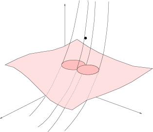
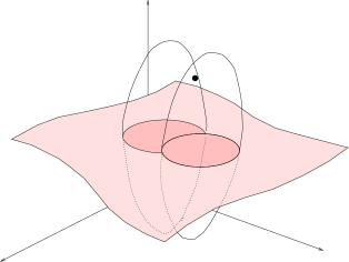
Figure 2: Approximate shapes of the acceptance regions for two near parameter points in the FC case (left) and in the CG case (right). In the first case the regions are stretched perpendicularly to the theoretical surface, while in the second they are ellipsoidal. A parameter point is accepted if the measured experimental point (black dot in the figures) lies inside its acceptance region.

The correct frequentist construction of the confidence regions is a well-known procedure: for any point $m$ in the parameter space ($\Delta m^{2}$ and $\theta$, in our case) one has to arbitrarily choose a region ${\cal{A}}(\mbox{\normalsize\boldmath$m$})$ in the space $\{\mbox{\normalsize\boldmath$x$}\}$ of the data (the three rates, in our case) which contains the CL% of the probability. The knowledge of the pdf (1) allows to do this. The confidence region ${\cal{B}}(\mbox{\normalsize\boldmath$x$})$ is given by all the points in the parameter space that contains the measured value of the experimental data in their acceptance region:

$${\cal{B}}(\mbox{\normalsize\boldmath$x$})=\{\mbox{\normalsize\boldmath$m$}|\mbox{\normalsize\boldmath$x$}\in{\cal{A}}(\mbox{\normalsize\boldmath$m$})\}.$$ (5)

It is easy to realize that, taken any true value for the parameters, the quoted region contains this true value in the CL% of the cases.

The arbitrariness in the choice of the acceptance region ${\cal{A}}(\mbox{\normalsize\boldmath$m$})$ can be fixed by choosing a particular ordering in the data space: the construction of ${\cal{A}}(\mbox{\normalsize\boldmath$m$})$ is made adding $x$-cells in that order until the requested probability (coverage) is reached. Crow and Gardner (CG) proposed [12] an ordering based on $p(\mbox{\normalsize\boldmath$x$}|\mbox{\normalsize\boldmath$m$})$, while Feldman and Cousins (FC) proposed [13] an ordering based on the likelihood ratio

$$p(\mbox{\normalsize\boldmath$x$}|\mbox{\normalsize\boldmath$m$})/p(\mbox{\normalsize\boldmath$x$}|\mbox{\normalsize\boldmath$m$}_{\rm best}(\mbox{\normalsize\boldmath$x$})).$$ (6)

This means that the ‘priority’ of a point $x$ for fixed $m$ is given by its probability relative to the probability obtained with the parameters set at the best-fit value $\mbox{\normalsize\boldmath$m$}_{\rm best}(\mbox{\normalsize\boldmath$x$})$ corresponding to $x$.

2.1 Feldman–Cousins fit

The FC ordering requires cumbersome numerical computations, but guarantees that the FC acceptance regions share the nice properties of the approximate $\Delta\chi^{2}$-cut method. The FC ordering disregards the statistical fluctuations with no information on the parameters. If the measured rates are unlikely for any value of the parameters, the FC procedure “renormalizes” the probability when determining the confidence regions. It is easy to see that the FC acceptance regions are never empty for any choice of the confidence level: every point in the data space belongs at least to the FC acceptance region of the parameter $\mbox{\normalsize\boldmath$m$}_{\rm best}$ that maximizes its probability.

The FC procedure has many points in common with the approximate $\Delta\chi^{2}$-cut method: looking at eq.s (2)–(4) at fixed $m$ we see that the inequality $\lambda<\beta$ chooses ${\cal{A}}(\mbox{\normalsize\boldmath$m$})$ with the same ordering as the FC method. The only difference is that the limit $\beta$ is chosen, using the asymptotic distribution of $\lambda$, independent of $m$, while the exact method gives a limit $\beta(\mbox{\normalsize\boldmath$m$})$ that depends on the oscillation parameters $m$.

It is easy to check that the $\Delta\chi^{2}$-cut is exactly equivalent to the FC construction if the pdf is Gaussian with constant covariance matrix and with theoretical rates that depend linearly on the parameters (by ‘theoretical rates’ we indicate the most likely value of the rates, for given values of $\Delta m^{2}$ and $\theta$). In the linear approximation the theoretical rates, obtained varying the two parameters $\Delta m^{2}$ and $\theta$, form a plane in the three dimensional space of the rates. The comparison with this linear approximation helps us to understand whether the $\Delta\chi^{2}$-cut is a good approximation. Two different behaviors are possible for a given $m$:

• The value of $\beta(\mbox{\normalsize\boldmath$m$})$ given by the FC procedure is smaller than the approximated one derived by the $\Delta\chi^{2}$-cut. This happens, for example, if we measure values of the parameters near the edges of the parameter space. The $\Delta\chi^{2}$ approximation assumes an infinite hyperplane of theoretical rates: the points of the data space that have maximal probability for ‘non-physical’ values of the parameters will be included in the acceptance regions of the points near the edge, reducing their limit $\beta$ to have a correct coverage.

• The value of $\beta(\mbox{\normalsize\boldmath$m$})$ is larger than the approximated one. This happens when different regions of the parameter space give similar predictions for the data. A data point that is included in the acceptance region of a given $m$ in the linear approximation may have a bigger $p(\mbox{\normalsize\boldmath$x$}|\mbox{\normalsize\boldmath$m$}_{\rm best})$ because of the folding of the hypersurface, which lowers its likelihood ratio. To reach the requested probability a bigger value for $\beta$ is needed.

Within the LMA, LOW and SMA regions the linear approximation is pretty good, as the curvature of the ‘theoretical surface’ is small with respect to the typical errors on the rates. The effects due to the edges of the theoretical surface can also be neglected. The main deviation from the $\Delta\chi^{2}$ approximation is due to the fact that SMA, LMA, LOW points give similar predictions: the surface of theoretical rates is folded. Constructing the acceptance region for an oscillation parameter $m$ in the SMA region, we find points with best-fit parameters in the LMA region, so that the $\Delta\chi^{2}$ approximation is expected to give some undercoverage. The FC acceptance regions at $90\%$ and $99\%$ CL are plotted in figure 1: we see that the regions obtained from the $\Delta\chi^{2}$-cut are smaller than the exact FC regions. For example, the approximated $\Delta\chi^{2}$ cut at 90% CL is $\Delta\chi^{2}<4.6$. The value of $\beta(\mbox{\normalsize\boldmath$m$})$ at 90% CL obtained with the FC construction is $\approx(4.6\div 5.5)$ for $m$ in the SMA region and $\approx(4.8\div 5.5)$ for $m$ in the LMA region. Furthermore, owing to the variation of $\log\det\sigma^{2}$ (neglected by the $\Delta\chi^{2}$ approximation), in the SMA and LOW regions the FC boundary intersects the $\Delta\chi^{2}$ boundary, instead of surrounding it. The difference between the approximate and rigorous methods is however small enough to justify the $\Delta\chi^{2}$ approximation.

2.2 Crow–Gardner fit

A second way to construct confidence regions is based on the CG ordering: the acceptance regions are built beginning from the points of highest probability. Such ordering is not invariant under a reparametrization of the experimental data (e.g. a CG fit of the rates is different from a CG fit of the squared rates). Such acceptance regions are the smallest with the given coverage. The difference between the FC and the CG procedures is essential for those points that are unlikely for any value of the parameters, i.e. all the points far from the surface of theoretical rates. We have seen that, with the FC ordering, every data point is included in the acceptance region of at least one point in the parameter space, but this is obviously not true for the CG method. Consider for example the linear approximation in which the theoretical rates describe a plane in the rate space. For a given $m$, in view of (1), the CG acceptance region will be an ellipsoid centered in the most likely value for the rates, which becomes larger and larger with growing CL. The FC acceptance regions will be very different and stretched to infinity in a cylindrical shape perpendicularly to the plane (see figure 2). This is clear if we consider that in this approximation the maximum likelihood point $\mbox{\normalsize\boldmath$m$}_{\rm best}$ is obtained by projecting a data point on the ‘theoretical plane’ (in the base where the covariance matrix is proportional to the identity): all the points lying on a line perpendicular to this plane and intersecting it in the point described by $m$ have likelihood ratio equal to 1 and are included in the acceptance region.

Figure 3: Comparison between the CG acceptance region (black) and the FC one (red) at 90% CL for a parameter point in the SMA region. Chlorine and Gallium rates are in SNU, while the SK rate is in $10^{6}\,{\rm cm}^{-2}{\rm s}^{-1}$. The presence of LMA points with comparable predictions makes the FC region asymmetric and disconnected.

In figure 3 we compare the FC and CG acceptance regions for one given SMA oscillation. We see that the CG region is ellipsoidal as expected, while the FC one is stretched, but in one direction only. This is due to the strong non-linearity of the ‘theoretical surface’: LMA and SMA have similar rate predictions even if they have very different parameters. The surface is folded and this causes the asymmetry in the FC region: the acceptance region is deformed and disconnected to get far from the LMA predictions.

The CG acceptance regions at $90\%$ and $99\%$ CL are plotted in figure 1. The differences between the FC and CG confidence regions are readily understood. If we fix the experimental data and begin from a very low CL, we expect an empty CG region (there is no ellipsoid that contains the data) while the FC region is small but non empty. As the CL increases, a CG region appears (roughly at 4% CL in our case) and all the regions grow. With a large CL we expect the CG regions to be larger than the FC ones as the ellipsoids have a larger projection on the ‘theoretical surface’ than the stretched FC acceptance regions (see fig. 2). All these features can be checked explicitly in figure 1.

In conclusion two points must be stressed: first of all we have checked that a correct frequentist approach gives results only slightly different from the naive analysis based on the $\Delta\chi^{2}$-cut. This is apparently in contrast to what is obtained in [14]. The main difference between that analysis and ours is that we use all three rates to construct confidence regions, while [14] finds, with a Monte Carlo simulation, the distribution of the maximum likelihood estimators $\Delta\hat{m}^{2}$ and $\hat{\theta}$ and construct from this the confidence regions, using the Crow–Gardner ordering. Since the two $\Delta\hat{m}^{2}$, $\hat{\theta}$ are not a sufficient statistics for the three rates, this procedure implies a certain loss of information, which leads to larger confidence regions.

A second point is the comparison between the two methods, CG and FC: the results are pretty similar. As we will see in the next section, this is no longer the case when the SK data on the angular and energy distribution are included in the fit. We have not shown ‘vacuum oscillation’ fits of the solar rates because they are strongly disfavoured by the SK data.

3 The inclusion of the whole data set

The SuperKamiokande collaboration has also measured the energy spectrum of the recoil electrons as a function of the zenith-angle position of the sun. The full data set usually employed in solar neutrino fits contains 38 independent dof (see the appendix). With such a number of data it is practically impossible to perform a complete numerical construction of the acceptance regions, without any approximation. For example, even if we divide every dimension of the data space in only 20 cells, we arrive to a 38-dimensional space divided into $\sim 10^{50}$ cells. For this reason we cannot construct the FC confidence regions with all the data set. However, for the same reasons described in the previous section, the approximated $\Delta\chi^{2}$-cut method is expected to be a reasonable approximation of the FC construction and to give confidence regions slightly smaller than the FC ones.

For the CG ordering the situation is better. Since we have approximated the pdf (1) as a Gaussian function of the data, the CG construction is equivalent to a cut on the $\chi^{2}$ with 38 dof (rather than on the $\Delta\chi^{2}$). Note that in this case the procedure is exact even if $\log\det\sigma^{2}$ is not constant. For any $m$ the $\chi^{2}$-cut defines an ellipsoidal acceptance region ${\cal{A}(\mbox{\normalsize\boldmath$m$})}$, and the confidence region is given by the set of parameters with $\chi^{2}$ smaller than a given value. The comparison between the CG ordering and the approximated $\Delta\chi^{2}$-cut can be done analytically: for any given value of CL

$$\begin{array}[]{lrl}{\rm FC}~{}\approx\Delta\chi^{2}{\rm-cut}:&\chi^{2}(\Delta m^{2};\theta)-\chi^{2}_{\rm best}&\leq{\rm Quantile}(\chi^{2}_{\rm\>2\>dof},{\rm CL})\\ {\rm CG}~{}=\chi^{2}{\rm-cut}:&\chi^{2}(\Delta m^{2};\theta)&\leq{\rm Quantile}(\chi^{2}_{\rm\>38\>dof},{\rm CL}).\end{array}$$ (7)

The comparison between the CG method and the $\Delta\chi^{2}$-cut, which we can consider an approximation of the FC ordering, is shown in figure 4 and presents all the features described in the previous section. The differences are now rather evident. The CG regions are empty until the $\approx$ 40% CL, while the $\Delta\chi^{2}$ regions are never empty (as the FC ones). The two methods give equal regions for $\sim$ 45% CL. With a larger CL the CG regions are bigger than the $\Delta\chi^{2}$ regions. Figure 4 shows that the arbitrariness in constructing frequentist acceptance regions can be quite significant. For example a CG fit accepts a large $\Delta m^{2}\approx 10^{-3}{\rm eV}^{2}$ at $\approx 75\%$ CL, while the $\Delta\chi^{2}$ approximation to the FC fit rules it out at $\approx 98\%$ CL. One should keep in mind the statistical assumptions behind this limit, when using it to demonstrate the necessity of a hierarchy between the squared-mass differences characteristic of the solar and atmospheric anomalies. We now explain the reason of this difference and argue that the FC fit is the relevant one.

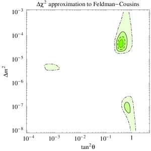
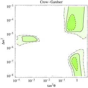
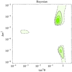
Figure 4: Comparison between the $\Delta\chi^{2}$-cut (left), the CG method (middle) and a Bayesian fit done assuming a flat prior in the plotted variables (right). We show the 35% (dotted lines), 68% (dashed), 90% (continuous) and 99% CL (dot-dashed) regions.

It could seem strange that, after including all data, the CG confidence regions with high CL are much larger than when fitting only the rates. This happens because the CG method does not use the information on the parameters contained in the data in the most efficient way. Statistical fluctuation leads to experimental results that do not lie on the theoretical surface. The CG ordering, treating in the same way the directions in the data space ‘perpendicular” and ‘parallel’ to the surface, does not use the information contained in the ‘distance’ from the theoretical surface to obtain further information on the parameters. This is why the CG ordering leads to strange results, though correct from the coverage point of view. The FC method uses the ‘distance’ from the theoretical surface to recognize and eliminate the statistical fluctuations that have nothing to do with the determination of the parameters. This difference between the two procedures is much more significant when fitting the full data set than when fitting the rates only. There are now many more data than unknown parameters: the theoretical surface is two-dimensional in a 38-dimensional data space.

In figure 4 we also show a Bayesian fit, done assuming a flat prior $dp(\Delta m^{2},\theta)=d\ln\Delta m^{2}\,d\ln\tan\theta$. Unlike the CG fit, this Bayesian fit should coincide with the $\Delta\chi^{2}$ approximation to the FC fit if the pdf were a Gaussian function of $\ln\Delta m^{2}$ and $\ln\tan\theta$. By comparing the two fits we can again see visible but not crucial corrections due to the non-Gaussianity in the theoretical parameters $\Delta m,\theta$. The arbitrariness in the prior distribution function $p(\Delta m^{2},\theta)$ gives an uncertainty comparable to the effect due to the non-Gaussianity.

4 The goodness of fit

A goodness-of-fit (GOF) test studies the probability of the experimental data $p({\rm data}|{\rm theory})$ under given theoretical hypotheses (a model of the sun, the assumption that neutrinos are oscillating rather than decaying…) leading to statements of the form: if all the hypotheses are true, the probability that the discrepancy between predictions and data is due to statistical fluctuations is less than a certain amount. The purpose is to understand if the theoretical hypotheses used to explain the data are plausible or not.

$$\begin{array}[]{c|ccc}\parbox[c]{56.9055pt}{\centering Goodness\\ of fit\@add@centering}&\hbox{($a$) Rates only}&\parbox[c]{113.81102pt}{($b$) Rates and spectra:\\ \phantom{(b) }naive result}&\parbox[c]{113.81102pt}{($c$) Rates and spectra:\\ \phantom{(c) }refined result}\\ \hline\cr\rm SMA&55\%(58\%\cite[cite]{[\@@bibref{}{recentfits1}{}{}]},50\%\cite[cite]{[\@@bibref{}{recentfits2}{}{}]},51.8\%\cite[cite]{[\@@bibref{}{giunti}{}{}]})&30\%~{}(34\%\cite[cite]{[\@@bibref{}{recentfits2}{}{}]})&\,\raise 1.29167pt\hbox{$<$\kern-7.5pt\lower 4.30554pt\hbox{$\sim$}}\,~{}2\,\%\\ \rm LMA&~{}6\%(10\%\cite[cite]{[\@@bibref{}{recentfits1}{}{}]},~{}8\%\cite[cite]{[\@@bibref{}{recentfits2}{}{}]},6.3\%\cite[cite]{[\@@bibref{}{giunti}{}{}]})&60\%~{}(59\%\cite[cite]{[\@@bibref{}{recentfits2}{}{}]})&\,\raise 1.29167pt\hbox{$<$\kern-7.5pt\lower 4.30554pt\hbox{$\sim$}}\,15\,\%\\ \rm LOW&0.7\%(1.6\%\cite[cite]{[\@@bibref{}{recentfits1}{}{}]},0.5\%\cite[cite]{[\@@bibref{}{recentfits2}{}{}]},1.1\%\cite[cite]{[\@@bibref{}{giunti}{}{}]})&50\%~{}(40\%\cite[cite]{[\@@bibref{}{recentfits2}{}{}]})&\,\raise 1.29167pt\hbox{$<$\kern-7.5pt\lower 4.30554pt\hbox{$\sim$}}\,~{}2\,\%\\ \rm\hbox{$P_{ee}={\rm cte}$}&0.3\%&28\%&\,\raise 1.29167pt\hbox{$<$\kern-7.5pt\lower 4.30554pt\hbox{$\sim$}}\,~{}1\,\%\end{array}$$

Table 1: GOF of the SMA, LMA, LOW and energy-independent solutions obtained by fitting (a) only the rates, (b) including all the data, (c) including only the ‘most significant’ data. The energy-independent solution contains only one free parameter, while SMA, LMA, LOW have two free parameters. Our results are compared with the corresponding ones in [22, 23, 14]. The symbol  $<$$\sim$  recalls that the GOF values could be slightly lower.

When analyzing the most recent data, one encounters the following paradoxical situation: the LOW solution gives a poor fit of the solar rates only (e.g. [23] finds a GOF of $0.5\%$). After including the full data set, LOW gives a good fit (e.g. [23] finds a GOF of $40\%$). The paradox is that we have added 35 zenith and energy bins, in which there is no signal for neutrino oscillations. It is clearly necessary to understand better the meaning of the GOF test before we can decide if LOW gives a decent fit or not. This important question also applies to the other alternative solutions. Such tests are based on Pearson’s $\chi^{2}$: the quantity [20]

$$\sum_{ij}(x_{i}^{\rm exp}-\hat{x}_{i}^{\rm th})\hat{\sigma}^{-2}_{ij}(x_{j}^{\rm exp}-\hat{x}_{j}^{\rm th})$$ (8)

is asymptotically distributed as a $\chi^{2}$ with $N_{\rm data}-N_{\rm param}$ dof. The hats indicate that the corresponding quantity must be evaluated at the maximum likelihood parameter point. The CG ordering is deeply linked to this GOF test: the absence of a confidence region until a given CL value is correlated to the goodness of the fit.

The paradoxical increase of the GOF of LOW is clearly due to the fact that the Pearson test does not recognize that there is a problem concentrated in the three solar rates that contain all the evidence for neutrino oscillations. It only sees that the total $\chi^{2}$ is roughly equal to the large total number of dof (38), so that the fit seems good. According to this procedure, even a global three neutrino fit of solar, atmospheric and LSND data would seem good. It is well known that the LSND anomaly requires a fourth neutrino, or something else.

We now explain why the Pearson’s test is not adequate for such a situation. Pearson’s test does a precise thing: it tests the validity of a certain solution with respect to a generic alternative hypothesis, which has a sufficient number of parameters to fit all the data with infinite precision. Therefore the inclusion of more data changes also the set of alternative hypotheses which we compare with. Describing the recoil electron spectrum in terms of 18 energy bins implies that we admit alternative theories with fuzzy energy spectra. No physical mechanism could generate an irregular spectrum, so that we do not want to test this aspect. The measured spectrum is of course regular, and Pearson test rewards the LOW solution for this reason. To better understand this point, suppose that we add as new data the direction of arrival of the interacting neutrinos. All solutions (including the no-oscillation hypothesis) would have a higher GOF. It is obvious that these solutions are much better than a generic one, because they at least ‘know’ where the Sun is. A meaningful $\chi^{2}$ test should include only those data that really test the hypothesis under consideration. On the contrary, the inclusion of irrelevant data does not affect the confidence regions built with the FC ordering, so that a naive application of the $\Delta\chi^{2}$-cut correctly approximates the best-fit regions.

We therefore conclude that testing the goodness of the fit using a lot of energy bins gives a formally correct answer to an irrelevant question. If a smaller set of data were used to describe the spectral and angular information, the set of alternative hypotheses would be more reasonable and one would conclude that there is a goodness-of-fit problem. Most of the information on the energy and zenith-angle spectra can be condensed into observables such as the mean recoil electron energy and the day/night asymmetry, as shown in fits presented by the SK collaboration [4].

Within our assumption of 2-neutrino oscillations, the main new information encoded in SK spectral and day/night data is that the survival probability $P_{ee}(E_{\nu})$ can only have a mild energy dependence around $E_{\nu}\sim 10\,{\rm MeV}$. This can be seen in a simple way by parameterizing $P_{ee}(E_{\nu})$ as

$$P_{ee}(E_{\nu})=P_{0}+P^{\prime}_{0}\cdot\bigg{(}\frac{E_{\nu}}{10\,{\rm MeV}}-1\bigg{)}+\frac{P^{\prime\prime}_{0}}{2}\bigg{(}\frac{E_{\nu}}{10\,{\rm MeV}}-1\bigg{)}^{\!\!2}+\cdots$$ (9)

The SK spectral data measure $P^{\prime}_{0}=-0.05\pm 0.1$ and disfavour the SMA solution because it prefers a larger slope $P^{\prime}_{0}$. Significant non-linearities in $P_{ee}(E_{\nu})$ are not predicted in SMA, LMA, LOW oscillations, nor could be recognized by SK (the present error on $P^{\prime\prime}_{0}$ is $\sim 1$).

In conclusion most of the information contained in the SK spectral data can be conveniently condensed into a single observable $f$, that measures the slope of $P_{ee}(E_{\nu})$. One possible choice is the ratio between the rate of ‘low energy’ (i.e. $T_{e}<9\,{\rm MeV}$) and ‘high energy’ (i.e. $9\,{\rm MeV}<T_{e}<13\,{\rm MeV}$) recoil electrons, as measured by SK. The upper bound on the recoil electron energy $T_{e}$ has been chosen in order to avoid potential problems due to an enhanced flux of h$e$p neutrinos. The measured value and the uncertainty on $f(\rho_{i})$ can be easily deduced from the SK data on the full energy spectrum: $\sigma^{2}_{f}=f_{i}\sigma_{ij}^{2}f_{j}$ (in Gaussian approximation), where $f_{i}\equiv\partial f/\partial\rho_{i}$, $\{\rho_{i}\}$ is the full set of SK bins and $\sigma^{2}_{ij}$ is the full error matrix.

By supplementing the fit of the total neutrino rates with a single observable $f$ we find the GOF values shown in table 1. The symbol  $<$$\sim$  recalls that, especially in the SMA case, it could be possible to obtain slightly lower GOF values by identifying another observable more sensitive to the energy dependence of the neutrino survival probability. However, a variation of the GOF between, say, $1\%$ and $4\%$, is within the uncertainty due to arbitrariness inherent in any statistical analysis. The important point is that the GOF values are significantly lower than the values based on a naive $\chi^{2}$ test, and motivate a non-standard analysis of the solar neutrino anomaly [24]. The SK collaboration [2] finds that SMA now gives a poor fit using another reasonable procedure: at 97% CL, the region favoured by total rates falls inside the region disfavoured by spectral and day/night data.

5 Conclusions

Fits of solar neutrino data are usually done using the $\Delta\chi^{2}$-cut valid in the Gaussian approximation and find few distinct best-fit solutions (LMA, SMA, LOW, …). Since a Gaussian would have only one peak, it is useful to check the validity of the $\Delta\chi^{2}$-cut approximation by comparing its results with the exact confidence regions built using the Neyman construction. This has been done using two different ordering prescriptions, proposed by Crow–Gardner (CG) and by Feldman–Cousins (FC). We find that the $\Delta\chi^{2}$ cut provides a good approximation to the Feldman–Cousins confidence regions.

When the full data set is used, there is some significant difference between the CG and FC regions. Even if the two methods give regions with the same statistical meaning, their conceptual significance is different. The FC regions are not influenced by statistical fluctuations with no information on the oscillation parameters, while the CG regions are composed by all the oscillation parameters that provide an acceptable fit of the data. The meaning of the results is deeply influenced by the assumptions involved in the statistical analysis. We finally show that a correct understanding of the meaning of Pearson ‘goodness-of-fit’ test invalidates the statement that all solutions (LMA, LOW and SMA) presently give a good fit.

We hope that our refined statistical analysis has been useful for clarifying some aspects of solar neutrino fits. Only refined experimental data will allow to identify the solution of the solar neutrino problem. We plan to update the electronic version of this paper, if new significant experimental data will soon be presented.

90% CL                                                             99% CL

Figure 5: The ‘rates only’ fit of fig. 1, updated including the SNO results. Confidence regions at 90% (left) and 99% (right) CL obtained from the four solar rates using three different methods: the $\Delta\chi^{2}$ approximation (continuous line), the Feldman–Cousins procedure (dashed line) and the Crow–Gardner procedure (dotted line).

Figure 6: The ‘global’ fit of fig. 4, updated including the SNO results. Comparison between the the CG method (left), the $\Delta\chi^{2}$-cut (middle), and a Bayesian fit done assuming a flat prior in the plotted variables (right). We show the 35% (dotted lines), 68% (dashed), 90% (continuous) and 99% CL (dot-dashed) regions.

6 Addendum: CC SNO results

In this addendum, we update our results by adding:

• the $\nu_{e}{\rm d}\to{\rm pp}e$ (CC) rate measured at SNO [29] above the energy threshold $T_{\rm eff}>6.75\,{\rm MeV}$: $R_{\rm SNO}^{\rm CC}=(1.75\pm 0.13)10^{6}\,{\rm cm}^{-2}{\rm s}^{-1}$.

• the latest SK results [30] (1258 days). The total flux now is $R_{\rm SK}=(2.32\pm 0.08)\cdot 10^{6}\,{\rm cm}^{-2}{\rm s}^{-1}$. The day/night energy spectrum contains a new bin with energy $5\,{\rm MeV}<E_{e}<5.5\,{\rm MeV}$.

• Furthermore, we explicitly include the CHOOZ data [15] in the global fit. CHOOZ data just disfavour values of $\Delta m^{2}$ above $0.7~{}10^{-3}{\rm eV}^{2}$ for large mixing $\theta\sim\pi/4$ and are irrelevant at smaller $\Delta m^{2},\theta$.

The updated fit of the four Chlorine, Gallium, SK and SNO rates (without including spectral data) is shown in fig. 5. The Feldman-Cousins SMA region is somewhat smaller than what obtained from the $\Delta\chi^{2}$ approximation: this is mainly due to the variation of the determinant of the covariance matrix in the SMA region (see section 2). Anyway there is no significant discrepancy between the frequentist fits and the $\Delta\chi^{2}$ Gaussian approximation.

Fig. 6 shows the results for the global fit, including all the rates and the day/night spectrum measured by SK. The Crow-Gardner (CG) confidence regions are composed by all oscillation parameters with a high goodness-of-fit, evaluated in a naïve way. As explained in section 3 the CG procedure gives very large confidence regions because it is an inefficient (although statistically correct) procedure. The Feldman-Cousins (FC) procedure gives smaller regions because it is more efficient: unlike the CG procedure it recognizes and eliminates the statistical fluctuations with no information on the oscillation parameters. In the Gaussian approximation, it should agree with the Bayesian fit with flat prior distribution: the differences between the $\Delta\chi^{2}$-approximation and the Bayesian are visible in fig. 6 but not significant.

How strongly is now the SMA solution disfavoured? Remembering that the difference in the best-fit ${\chi}^{2}$ is a powerful statistical indicator, the main results can be summarized as

$$\hat{\chi}^{2}({\rm SMA})=\hat{\chi}^{2}({\rm LMA})+\left\{\begin{array}[]{ll}14.0&\hbox{our fit}\cr 14.7&\cite[cite]{[\@@bibref{}{LisiSNO}{}{}]}\cr 10.1&\cite[cite]{[\@@bibref{}{BPGSNO}{}{}]}\cr 11.2&\cite[cite]{[\@@bibref{}{indiaSNO}{}{}]}\end{array}\right.,\qquad\hat{\chi}^{2}({\rm LOW})=\hat{\chi}^{2}({\rm LMA})+\left\{\begin{array}[]{ll}3.2&\hbox{our fit}\cr 4.5&\cite[cite]{[\@@bibref{}{LisiSNO}{}{}]}\cr 3.1&\cite[cite]{[\@@bibref{}{BPGSNO}{}{}]}\cr 4.4&\cite[cite]{[\@@bibref{}{indiaSNO}{}{}]}\end{array}\right.$$ (10)

where, for comparison, we also report the results of three other post-SNO analyses. Like in [32] and unlike in [31, 33] we improved the definition of the $\chi^{2}$ by using as data the SK flux in the $18+18$ energy day/night bins, rather than separating the SK data into total flux and un-normalized spectrum. This improved $\chi^{2}$ takes into account statistical correlations between the total SNO and SK rates and the SK spectral data. Due to the different energy thresholds in SK and SNO such kind of correlations are now non negligible: using the improved $\chi^{2}$ the difference $\Delta\hat{\chi}^{2}\equiv\hat{\chi}^{2}({\rm SMA})-\hat{\chi}^{2}({\rm LMA})$ is reduced by $\sim 3$. A MonteCarlo simulation would be necessary to determine precisely how $\Delta\hat{\chi}^{2}$ is distributed: presumably (10) implies that the evidence for LMA against SMA is now somewhere between “$3\sigma$” and “$4\sigma$”.

As discussed in section 4, the claims in [32, 33] that the SMA solution (and few other disfavoured solutions) still give a ‘good fit’ is based on an inefficient goodness-of-fit test on the value of some global $\chi^{2}$. In the case of parameter determination, the Crow-Gardner procedure is statistically correct (like the global $\chi^{2}$ test), but no one employs it just because it is inefficient (as clear in fig. 6). Using the more efficient goodness-of-fit test discussed in section 4, we get the updated post-SNO results

$$\hbox{GOF(LMA)}\sim 25\%,\qquad\hbox{GOF(LOW)}\sim 4\%,\qquad\hbox{GOF(EI)}\sim 1\%,\qquad\hbox{GOF(SMA)}\sim 0.4\%,$$

where EI denotes the ‘energy independent’ solution obtained for $\Delta m^{2}\,\raise 1.29167pt\hbox{$>$\kern-7.5pt\lower 4.30554pt\hbox{$\sim$}}\,2\cdot 10^{-4}{\rm eV}^{2}$. Unlike few years ago LMA, LOW or EI oscillations are now better than SMA not because new data gave new significant positive indications for them, but because new data (compatible with no spectral distortion) gave a strong evidence against SMA. The ‘worse’ solutions of few years ago are now the ‘better’ ones, but cannot give very good fits. Of course all results in this paper are based on the (sometimes questionable) assumption that all systematic and theoretical uncertainties involved in the game have been correctly estimated. The final results do not significantly change if the (not yet calibrated) Chlorine result is not included in the fit.

Figure 7: Regions ‘favoured’ (green) and ‘disfavoured’ (red) by the first SNO data.

In order to show in more detail the impact of SNO, in fig. 7 we plot the values of the variation in the $\chi^{2}$ due to the SNO data:

$$\Delta\chi^{2}=\chi^{2}(\hbox{post-SNO})-\chi^{2}(\hbox{pre-SNO}).$$

We see again that SNO results perfectly agree with LMA and LOW (for the value of the Boron flux predicted by solar models) and disfavour the SMA solution. Energy-independent solutions are also slightly disfavoured with respect to LMA and LOW: neglecting possible small corrections due to $\theta_{13}$, energy-independent oscillations can at most convert half of the initial $\nu_{e}$ into $\nu_{\mu},\nu_{\tau}$ (for maximal mixing), while SNO and SK indicate that the $\nu_{\mu},\nu_{\tau}$ flux is $\sim 1.5$ standard deviation higher than the $\nu_{e}$ flux.

Finally, it is useful to recall another important result: performing a global analysis including all experimental data (solar, atmospheric, reactor, short-baseline) in models with a fourth sterile neutrino, the best $\chi^{2}$ is obtained when the sterile neutrino is not used at all (so that atmospheric and solar data are explained by oscillations into active neutrinos, while the LSND data are not explained). This means that the present LSND evidence [16] for effects due to a sterile neutrino is weaker than the present evidence of other experiments against it.

7 Addendum: NC and day/night SNO results

In this addendum, we update our results by adding:

• The $\nu{\rm d}\to\nu{\rm pn}$ (NC) and the $\nu_{e}{\rm d}\to{\rm pp}e$ (CC) rate measured at SNO [34] during the initial pure D₂O phase using events with measured Čerenkov energy, $T_{\rm eff}$, larger than $5\,{\rm MeV}$. Assuming an energy-independent survival probability, $0\leq P_{ee}\leq 1$, SNO claims

  $$\halign to=0.0pt{\@eqnsel\hskip\@centering$\displaystyle{#}$&\global\@eqcnt\@ne\hskip 2\arraycolsep\hfil${#}$\hfil& \global\@eqcnt\tw@\hskip 2\arraycolsep$\displaystyle{#}$\hfil&\llap{#}\cr 0.0pt plus 1000.0pt$\displaystyle{R_{\rm SNO}^{\rm CC} &10.0pt\hfil${=&10.0pt$\displaystyle{1.76\pm 0.06\hbox{(stat)}\pm 0.09\hbox{(syst}) ~{}10^{6}\,{\rm cm}^{-2}{\rm s}^{-1} = \Phi_{{}^{8}{\rm B}} P_{ee},\\ R_{\rm SNO}^{\rm NC} &\hbox to0.0pt{\hss=&5.09\pm 0.44\hbox{(stat)}\pm 0.46\hbox{(syst})~{}10^{6}\,{\rm cm}^{-2}{\rm s}^{-1}=\Phi_{{}^{8}{\rm B}}(1-\eta_{\rm s}(1-P_{ee}))&(11)\cr}}}}}$$

  (with some mild anti-correlation; $0\leq\eta_{\rm s}\leq 1$ is the eventual sterile fraction involved in solar oscillations) giving a a $5.1\sigma$ direct evidence for neutrino conversion, $R_{\rm SNO}^{\rm CC}/R_{\rm SNO}^{\rm NC}<1$. If there are no sterile neutrinos ($\eta_{\rm s}=0$) $R_{\rm SNO}^{\rm NC}=\Phi_{{}^{8}{\rm B}}$, confirming the solar model prediction for the Boron flux. Without assuming that $P_{ee}(E_{\nu})$ is energy-independent, the error considerably increases [34]

  $$R_{\rm SNO}^{\rm NC}=6.4\pm 1.6\hbox{(stat)}\pm 0.6\hbox{(syst})~{}10^{6}\,{\rm cm}^{-2}{\rm s}^{-1}.$$

  In order to make an oscillation fit one needs to extract $R^{\rm NC}_{\rm SNO}$ from the SNO data, taking into account the energy distortion predicted by oscillations. We do this using the data reported in fig. 2c of [34].

• The day/night asymmetries measured at SNO. Assuming oscillations of only active neutrinos, SNO extracts the $\nu_{e}$ asymmetry to be $A_{e}=7.0\%\pm 5.1\%$ [35]. At $E_{\nu}\sim 10\,{\rm MeV}$ earth matter effects are too large for $\Delta m^{2}$ values between LMA and LOW (that are therefore excluded) and are still present in the lower $\Delta m^{2}$ range of LMA (here the regeneration effect is larger at high energy and for neutrinos that cross a sizable part of the earth) and in the upper $\Delta m^{2}$ range of LOW (here the regeneration effect is larger at low energy and has a characteristic oscillating zenith angle behavior) [37]. Both SK and SNO see a $\sim 1.5\sigma$ hint for a regeneration effect, but neither SK nor SNO data show a statistically significant energy or zenith-angle dependence of the effect, that would allow to discriminate LMA from LOW.

• The latest SK results [38] (1496 days): the full zenith angle and energy distributions have now been released, so that SK data now disfavour more strongly oscillations parameters that give rise to detectable earth matter effects at SK (the lower part of the LMA solution and the upper part of the LOW solution). We use as SK data the rates in the 44 bins, whose content and uncertainties are precisely described in tables 1 and 2 of [38].

• The latest SAGE result [39]. The averaged Gallex/SAGE/GNO rate is now $R_{\rm Ga}=(72.4\pm 4.7)\,{\rm SNU}$ (in place of the older value in eq. (A)), making the LOW solution less disfavoured.

• According to solar models, the total flux of ${}^{8}{\rm B}$ neutrinos is proportional to $S_{17}(0)$ (that parameterizes the ${}^{7}{\rm Be}\,{\rm p}\to{}^{8}{}{\rm B}\,\gamma$ cross section at zero energy). New recent measurements

  $$S_{17}(0)=17.8\pm 1.3\,\rm{eV~{}b}~{}\cite[cite]{[\@@bibref{}{Davids}{}{}]},\qquad S_{17}(0)=22.3\pm 0.9\,\rm{eV~{}b}~{}\cite[cite]{[\@@bibref{}{Jung}{}{}]},\qquad S_{17}(0)=22.7\pm 1.2\,\rm{eV~{}b}~{}\cite[cite]{[\@@bibref{}{ISOLDE}{}{}]}$$

  do not fully agree. Therefore we still use $S_{17}(0)=19^{+4}_{-2}\,\rm{eV~{}b}$, as in BP00 [5]. After the SNO NC measurement, this arbitrary choice is relevant almost only in fits with sterile neutrinos.

The result of our global fit is shown in fig. 8a (capabilities of SNO have been discussed in [43]). The best fit lies in the LMA region

$$\hat{\chi}^{2}\hbox{(47~{}dof)}=33.0\qquad\hbox{at}\qquad\Delta m^{2}=10^{-4.1}{\rm eV}^{2},\qquad\tan^{2}\theta=+0.35.$$

The LOW solution begins to be significantly disfavoured, because the precise SNO determination of the ${}^{8}{\rm B}$ flux makes more statistically evident that LOW oscillations give a poor fit of the other rates:

$$\hat{\chi}^{2}_{\rm LOW}=\hat{\chi}^{2}_{\rm LMA}+8.1$$

(a difference of $10.7$ is found in [35], where the full SK zenith-angle/energy spectra are not employed). If LMA is the true solution, KamLand could confirm it within few months.

Figure 8: Best fit regions at $90$, $99$, $99.73\%$ CL assuming $\nu_{e}\leftrightarrow\nu_{\mu,\tau}$ oscillations. In fig. 8a we fit the Cl, Ga rates, the SK day/night and zenith angle spectra, the SNO NC and CC rates and day/night asymmetries and the CHOOZ energy spectrum, assuming the BP00 [5] solar model. In fig. 8b we drop the BP00 prediction for the Boron and Beryllium solar fluxes.

Figure 9: Fig. 9a: best-fit regions of the Boron flux and of the fraction $\eta_{\rm s}$ of sterile neutrino involved in solar oscillations at $90$ and $99\%$ CL (2 dof). Fig. 9b: fraction of sterile neutrino (1 dof) allowed in solar (continuous lines) and atmospheric (dashed line) oscillations: in both cases data prefer no sterile neutrino.

Unlike in older fits, the upper part of the LMA region (that in the two-neutrino context we are considering gives rise to energy-independent oscillations with $P_{ee}\geq 1/2$) is now disfavoured also by solar data alone (the inclusion of the CHOOZ constraint now only has little effect), since SNO suggests $P_{ee}<1/2$. This can be considered as the first hint for MSW effects [6].

Vacuum oscillations predicted spectral distortions not seen by SK. Before SNO, the remaining marginally allowed vacuum oscillation solution was ‘JustSo²’ (with $\Delta m^{2}\,\raise 1.29167pt\hbox{$<$\kern-7.5pt\lower 4.30554pt\hbox{$\sim$}}\,10^{-11}{\rm eV}^{2}$) that predicted $P_{ee}\approx 1$ (i.e. approximately no oscillations) at energies probed by SK and SNO. Oscillations with $\Delta m^{2}\,\raise 1.29167pt\hbox{$<$\kern-7.5pt\lower 4.30554pt\hbox{$\sim$}}\,10^{-9}{\rm eV}^{2}$ now give the relatively better vacuum oscillation fit; their $\chi^{2}$ is larger than in the best LMA fit by about 14.

In fig. 8b we show the results of a fit where we do not include the BP00 [5] predictions for the Boron and Beryllium fluxes: the best-fit regions do not significantly change. From the point of view of oscillation analyses, the Beryllium flux is now the most relevant, not fully safe, solar model prediction (see [24] for a discussion): according to BP00 [5] the percentage error on the Beryllium flux is only two times smaller than the one on the Boron flux. Since Beryllium and Boron neutrinos are generated by different scattering processes of ${}^{7}{\rm Be}$, the agreement of the Boron flux with SNO data suggests (but does not imply) a Beryllium flux also in agreement with solar models.

We now explain in simple terms which data eliminate the other solutions allowed in older fits.

Autopsy of no oscillations

The NC and CC data from SNO alone exclude this case at $5.1\sigma$. The statistical significance of the solar neutrino anomaly increases to $8\sigma$, according to our global fit.

Autopsy of small mixing angle oscillations

For small mixing angle and in the SK and SNO energy range, $E_{\nu}\sim(5\div 15)\,{\rm MeV}$, the $\nu_{e}$ survival probability is well approximated by the Landau-Zener level-crossing probability, $P_{ee}\approx e^{-\bar{E}/E_{\nu}}$, where $\bar{E}$ is a constant (fixed by the oscillation parameters and by the solar density gradient). In order to get $P_{ee}\sim 1/2$ as demanded by SNO and SK one needs to choose $\bar{E}\sim 10\,{\rm MeV}$. This implies $dP_{ee}/d\ln E_{\nu}\sim 1$, in contrast with the undistorted energy spectrum observed by SK (see eq. (9)) and SNO. Performing a global fit we find

$$\hat{\chi}^{2}({\rm SMA})=\hat{\chi}^{2}({\rm LMA})+23$$

i.e. a $\,\raise 1.29167pt\hbox{$>$\kern-7.5pt\lower 4.30554pt\hbox{$\sim$}}\,4\sigma$ evidence for LMA versus SMA. As explained in section 4, the fact that $\chi^{2}/\hbox{dof}\approx 1.2$ for the SMA solution does not mean that SMA oscillations give a good fit: the Pearson’s $\chi^{2}$ test is not efficient in recognizing bad fits when there are many dof. A more efficient test (see sections 4 and 6) confirms that SMA has a low goodness-of-fit, as expected.

Autopsy of pure sterile oscillations

Assuming no distortion of the energy spectrum of Boron neutrinos, SNO sees a $5.1\sigma$ evidence for $\nu_{\mu,\tau}$ appearance. This evidence decreases down to $3\sigma$ allowing for generic spectral distortions, but significant spectral distortions are not allowed by SK. The sterile SMA solution (that gave the best sterile fit, before SNO) gives a spectral distortion that increases the SNO evidence for $\nu_{\mu,\tau}$ appearance, and is therefore excluded in two different ways. In our global fit we find

$$\hat{\chi}^{2}({\rm LMA~{}sterile})=\hat{\chi}^{2}({\rm LMA~{}active})+29.$$

SMA and LOW provide sterile fits slightly worse than LMA.

Autopsy of ‘2+2’ oscillations

The main motivation for adding a sterile neutrino, $\nu_{\rm s}$, is provided by the LSND anomaly. The extra neutrino can then be used to generate either the solar or atmospheric or LSND oscillations (so that active neutrinos can generate the remaining two anomalies). Only the last possibility is now not strongly disfavoured. In fact, taking into account that SK and MACRO atmospheric data give a $6\sigma$ evidence for $\nu_{\mu}\to\nu_{\tau}$ versus $\nu_{\mu}\to\nu_{\rm s}$ [45], it is no longer possible to fit the solar or atmospheric evidences (or one combination) with one sterile neutrino: ‘2+2’ schemes predict that the fraction of sterile involved in solar oscillations, plus the fraction of sterile involved in atmospheric oscillations, adds to one [44], but both solar and atmospheric data refuse sterile neutrinos. In fig. 9a we show how SK/SNO rates and solar model predictions for the Boron flux constrain the sterile fraction in solar oscillations. In fig. 9b we show how strongly data favor $\eta_{\rm s}\approx 0$ in both solar and atmospheric oscillations. The ‘number of standard deviations’ in fig. 9b is computed as $N_{\sigma}=[\chi^{2}(\eta_{\rm s})-\chi^{2}(\eta_{\rm s}=0)]^{1/2}$, where $\chi^{2}$ is minimized with respect to the Boron flux. Atmospheric bounds have been compiled from [45] (naïvely interpolating the few points given in [45]), where significant but unpublished data are employed. Solar bounds have been computed from SNO data alone (assuming an energy-independent $P_{ee}$), and from a global fit of all solar data. The result is not significantly different in the two cases, and depends on solar model uncertainties (e.g. the choice of $S_{17}$).

We remark that the bound on the sterile fraction holds in the case of active/sterile mixing at a $\Delta m^{2}\gg 10^{-3}{\rm eV}^{2}$, as suggested by the LSND anomaly. Active/sterile mixing with two small $\Delta m^{2}$ (e.g. one $\Delta m^{2}$ around $10^{-4}{\rm eV}^{2}$ and the other around $10^{-11}{\rm eV}^{2}$) could still give large effects at sub-MeV neutrino energies.

Acknowledgements

We thank Carlos Peña-Garay, Andrea Gambassi, Alberto Nicolis and Donato Nicolò for useful discussions. We thank Y. Suzuki for the unpublished SuperKamiokande data.

Appendix A Details of the computation

The energy spectra for the independent components of the solar neutrino flux have been obtained from [8]. The neutrino production has been averaged for each flux component over the position in the sun as predicted in [5, 8]. This averaging does not give significant corrections. MSW oscillations inside the sun have been taken into account in the following way. The $3\times 3$ density matrix $\rho_{S}$ for neutrinos exiting from the sun is computed using the Landau–Zener approximation with the level-crossing probability appropriate for an exponential density profile [6, 7]. The density profile has been taken from [8] and is quasi-exponential: small corrections to $\rho_{S}$ have been approximately included. Oscillation effects outside the sun are described by the evolution matrix $U$, so that at the detection point $\rho_{E}=U\rho_{S}U^{\dagger}$. In particular, earth regeneration effects have been computed numerically using the mantle-core approximation for the earth density profile. We have used the mean mantle density appropriate for each trajectory as predicted by the preliminary Earth model [25]. The detection cross sections in Gallium and Chlorine experiments have been taken from [8], performing appropriate interpolations. We have used the tree-level Standard Model expression for the neutrino/electron cross section at SK.

The total neutrino rates measured with the three kinds of experimental techniques are [1, 2, 3, 4]

$$\halign to=0.0pt{\@eqnsel\hskip\@centering$\displaystyle{#}$&\global\@eqcnt\@ne\hskip 2\arraycolsep\hfil${#}$\hfil& \global\@eqcnt\tw@\hskip 2\arraycolsep$\displaystyle{#}$\hfil&\llap{#}\cr 0.0pt plus 1000.0pt$\displaystyle{R_{\rm Cl}|_{\rm exp} &10.0pt\hfil${=&10.0pt$\displaystyle{(2.56\pm 0.22)\,{\rm SNU}\\ R_{\rm Ga}|_{\rm exp} &\hbox to0.0pt{\hss=&(74.7\pm 5)\,{\rm SNU}\\R_{\rm SK}|_{\rm exp}&=&(2.40\pm 0.08)\cdot 10^{6}\,{\rm cm}^{-2}{\rm s}^{-1}&(12)\cr}}}}}$$

where $\hbox{SNU}\equiv 10^{-36}\,\hbox{interactions per target atom and per second}$. We have combined systematic errors in quadrature with statistical errors. The probability distribution function $p({\rm data}|{\rm theory})$ is computed using the covariance matrix described in [9, 22]. Around the best-fits, it agrees well with the simpler pdf used in [24]. The experimental energy resolution at SK has been taken into account as suggested in [26, 27].

The solar-model-independent SK data included in the fit are the energy spectrum of the recoil electrons measured separately at SK during the day and during the night. Each energy spectrum [28] is composed of 17 energy bins between $5.5$ and $14\,{\rm MeV}$, plus one bin between $14$ and $20\,{\rm MeV}$. For these data we have used the pdf suggested by the SK collaboration [28], and described in [27] for a slightly different set of data.

The results presented in the addenda have been obtained using updated data and a slightly improved fitting procedure, as described in section 6 and 7.

8   Addendum: first KamLAND results

In this addendum, we update our results by adding the recently announced by KamLAND [1]. We also update our previous analysis including the most recent data from GNO and the full set of spectral and day/night SNO data. We here list the set of data included in our fit.

• Reactor anti-neutrino data (27 bins):

  • The KamLAND data, divided in 13 energy bins with prompt energy higher than $2.6\,{\rm MeV}$ [1].

  • The CHOOZ data, divided in 14 bins and fitted as in analysis “A” of [5].

• Solar neutrino data (80 bins):

  • The SNO data [6], divided in 34 bins (17 energy bins times 2 day/night bins).

  • The SuperKamiokande data [7], divided in 44 zenith-angle and energy bins.

  • The Gallium rate [8] $R_{\rm Ga}=(70.4\pm 4.4)\,{\rm SNU}$, obtained averaging the most recent SAGE, Gallex and GNO data.

  • The Chlorine rate [9] $R_{\rm Cl}=(2.56\pm 0.23)\,{\rm SNU}$.

• Solar model predictions. We assume the BP00 solar model [10] and its estimates of uncertainties.

• Earth matter effects are computed in the mantle/core approximation, improved by using the average density appropriate for each trajectory as predicted in [11].

We fit these data assuming $\nu_{e}\leftrightarrow\nu_{\mu,\tau}$ neutrino oscillations with a single $\Delta m^{2}$ and a mixing angle $\theta$. The total $\chi^{2}$ is obtained by summing the contribution from solar $\nu$ data, $\chi^{2}_{\nu}$, with the contribution from reactor $\bar{\nu}$ data, $\chi^{2}_{\bar{\nu}}=-2\ln{\cal L}$ (the likelihood ${\cal L}$ is computed employing when appropriate the Poissonian distribution). Best-fit regions are computed in Gaussian approximation, cutting the $\Delta\chi^{2}$ at the value appropriate for 2 degrees of freedom.

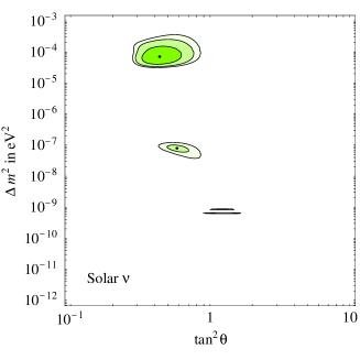
Figure 10: Best-fit regions at $90,~{}99$ and $99.73\%$ CL obtained fitting (a) solar $\nu$ data; (b) reactor $\bar{\nu}$ data (that do not distinguish $\theta$ from $\pi/2-\theta$); (c) all data (we find no other allowed regions at the considered CL outside the plotted range).

The result of our fit is shown in fig. 10. The best fit point (marked with a dot) and the $1\sigma$ ranges for the single parameters (1 dof) are

$$\Delta m^{2}_{12}=(7.0\pm 0.6)\,10^{-5}{\rm eV}^{2},\qquad\tan^{2}\theta_{12}=0.45\pm 0.06.$$

At the best fit point $\chi^{2}_{\nu}=72.9$ (80 bins) and $\chi^{2}_{\rm KamLAND}\approx 6$ (13 bins). The disfavoured local minimum at higher $\Delta m^{2}=1.53~{}10^{-4}{\rm eV}^{2}$ shown in fig. 10c (‘HLMA’ solution) has a $\chi^{2}$ 6.4 higher than in the best fit solution. According to our global fit, the combined evidence for a solar neutrino anomaly is almost $10\sigma$; the evidence for LMA versus SMA is about $6\sigma$; the QVO and LOW solutions are disfavoured at about $(4\div 5)\sigma$. According to a naïve Pearson $\chi^{2}$ test these excluded solutions still have an acceptable goodness-of-fit, around $20\%$ (this happens because the $\chi^{2}$ test has a limited statistical power when many data are fitted together, as we explained in section 4) while our more efficient test recognizes that their goodness-of-fit probability is $\sim 10^{-3}$. More importantly, present data are well described by LMA oscillations and do not contain hints for something more.

KamLAND data have an important impact also on various related issues:

• Maximal mixing? Fitting reactor data alone (fig. 10b), we find the best fit point at $\Delta m^{2}=6.9~{}10^{-5}{\rm eV}^{2}$, $\sin^{2}2\theta=0.99$ but also a larger uncertainty on the mixing angle $\theta$. Therefore maximal mixing remains disfavoured by solar data. In the global fit of fig. 10c, maximal mixing would enter the best-fit regions only at $99.96\%$ CL (2 dof). Before KamLAND, maximal mixing was allowed in Q(VO) solutions at a reasonable CL.

• Oscillations? If the present trend is confirmed by future KamLAND data, all proposed alternatives to oscillations will be excluded. If $\Delta m^{2}\,\raise 1.29167pt\hbox{$<$\kern-7.5pt\lower 4.30554pt\hbox{$\sim$}}\,2~{}10^{-4}{\rm eV}^{2}$, with more statistics KamLAND can see a clean oscillation pattern, giving a precise measurement of $\Delta m^{2}$ [12]. This will tell if earth-matter effects can be observed by a larger SK-like solar detector. At the best-fit point the total day/night asymmetry is predicted to be $2.7\%$ at SK and $4.5\%$ in CC events at SNO, comparable to present sensitivities.

• Future experiments. According to the present oscillation best-fit point, Borexino should observe no day/night asymmetry, no seasonal variation and a $65\%$ reduction of the ⁷Be flux. If this will happen, solar experiments alone will tell that LMA is the unique oscillation solution, confirming the CPT theorem. The impact of KamLAND data on our knowledge of solar neutrinos will be discussed in an update to [12]. Knowing that LMA oscillations are the solution to the solar neutrino anomaly allows to plan which experiment(s) will give the most precise measurement of $\Delta m^{2}$ and $\theta$ (see [14] and a future update).

• Three flavours. When analyzed in a three-neutrino context, solar and reactor experiments are also affected by atmospheric oscillations if $\theta_{13}\neq 0$. For the observed value of $\Delta m^{2}_{\rm atm}$, CHOOZ gives the dominant upper bound on $\theta_{13}$. Therefore setting $\theta_{13}=0$ is an excellent approximation for fitting solar data.

• Neutrino-less double-beta decay. Assuming hierarchical neutrinos $m_{1}\ll m_{2}\ll m_{3}$ the $ee$ element of the neutrino mass matrix probed by $0\nu 2\beta$ decay experiments can be written as $|m_{ee}|=|m_{ee}^{\rm sun}+e^{i\alpha}m_{ee}^{\rm atm}|$ where $\alpha$ is an unknown Majorana phase and the ‘solar’ and ‘atmospheric’ contributions can be predicted from oscillation data. Including KamLAND data, the solar contribution to $|m_{ee}|$ is $m_{ee}^{\rm sun}=(2.6\pm 0.4)~{}\,\hbox{meV}$. The CHOOZ bound on $\theta_{13}$ implies $m_{ee}^{\rm atm}<2\,\hbox{meV}$ at 99% CL.

• Sterile? Experimental bounds on a possible sterile neutrino component involved in solar oscillations are not yet significantly affected by KamLAND data, that instead have a strong impact on bounds from big-bang nucleosynthesis [13]. Such bounds cannot be avoided by modifying cosmology before neutrino decoupling and are usually presented in the $(\theta,\Delta m^{2})$ plane assuming pure sterile oscillations. It is now more interesting to know the bound on a possible subdominant sterile component involved in LMA solar oscillations. We estimate that this bound is competitive with the direct experimental bound.

• LSND. Solutions to the LSND anomaly based on extra sterile neutrinos are now disfavoured by other experiments [4]. The CPT-violating neutrino spectrum proposed in [16] allowed to fit all neutrino data, but predicted no effect in KamLAND. A slightly different CPT-violating solution mentioned in [4] can give a suppression in KamLAND at the price of an up/down asymmetry of atmospheric muon neutrinos $A\approx 20\%$, somewhat smaller than the measured value. This possibility is more disfavoured than ‘3+1 oscillations’ and less disfavoured than ‘2+2 oscillations’, as will be discussed in an update to [4].

Figure 11: Best-fit regions at $90,~{}99$ and $99.73\%$ CL obtained fitting (a) solar $\nu$ data; (b) reactor $\bar{\nu}$ data (that do not distinguish $\theta$ from $\pi/2-\theta$); (c) all data. These fits can be directly compared with the previous ones, shown in fig. 10.

9   Addendum: SNO data with enhanced NC sensitivity

SK detects solar $\nu$ using water as target. SNO now employs heavy salt water [1]. Heavy water allowed to study the NC reaction $\nu_{e,\mu,\tau}d\to\nu_{e,\mu,\tau}np$. Salt allows to tag the $n$ with higher efficiency (producing multiple $\gamma$ rays from neutron capture) and therefore a more accurate measurement of total solar $\nu_{e,\mu,\tau}$ flux. However, the enhanced NC signal makes more difficult to study the CC energy spectrum. As a consequence the recently released ‘salty’ SNO data [1] can be conveniently summarized as a measurement of the total CC, NC and electron scattering (ES) neutrino fluxes. Uncertainties on the Boron flux, its energy spectrum, and cross sections are correlated with other experiments. We fit latest SNO data as suggested by the SNO collaboration (this means that we are slightly less accurate than the SNO collaboration itself). We employ the most recent value of the Gallium rate [2].

The result of our fit is shown in fig. 11, where the best fit point is marked with a dot. The $1\sigma$ ranges for the single parameters (1 dof) are

$$\Delta m^{2}_{12}=(7.2\pm 0.7)\,10^{-5}{\rm eV}^{2},\qquad\tan^{2}\theta_{12}=0.44\pm 0.05.$$

At the best fit point $\chi^{2}_{\rm solar}=75.0$ (83 bins) and $\chi^{2}_{\rm KamLAND}\approx 6$. The total evidence for a solar anomaly is $12\sigma$ (dominated by solar experiments). We now discuss some consequences of latest SNO data:

• Oscillations? LMA solutions with larger $\Delta m^{2}$ (present in our previous fit of fig. 10c) have been disfavoured, because they predict a too large $\nu_{e}$ survival probability. This is important because only if $\Delta m^{2}\,\raise 1.29167pt\hbox{$<$\kern-7.5pt\lower 4.30554pt\hbox{$\sim$}}\,2~{}10^{-4}{\rm eV}^{2}$ KamLAND should be able, with more statistics, to see in the $\bar{\nu}_{e}$ energy spectrum the typical spectral distortion produced by oscillations and to measure $\Delta m^{2}$ accurately [3]. So far no experiment has been able of seeing such a direct signal of neutrino oscillations.

• Maximal mixing is disfavoured at $5.7\sigma$ (i.e. its $\chi^{2}$ is $5.7^{2}$ higher than the best LMA fit).

• Symmetry? $\tan^{2}\theta=1/2$ (which together with maximal $\nu_{\mu}\to\nu_{\tau}$ atmospheric oscillations gives a highly symmetric neutrino flavour composition, with $|\langle\nu_{e,\mu,\tau}|\nu_{2}\rangle|^{2}=1/3$) is $\sim 1.2\sigma$ above the best fit value. Hopefully, future data will test this special value.

• LMA. Omitting KamLAND $\bar{\nu}$ data and fitting only solar $\nu$ experiments, the LOW solution is now disfavoured at $3.3\sigma$: $0.5\sigma$ more than without SNO salt data. Other non-LMA oscillation solutions have now been excluded by solar data only.

• MSW effect. SNO gives a $5\sigma$ evidence for a $\nu_{e}$ survival probability less than $1/2$. This can be explained by MSW enhancement of neutrino oscillations [8], while averaged vacuum oscillations of two-neutrinos can only give $P_{ee}=1-\frac{1}{2}\sin^{2}2\theta\geq 1/2$ (see also [4]). Three-neutrino mixing can only marginally reduce $P_{ee}$, since SK and SNO imply that $\theta_{13}$ is small.

• Three flavours. When analyzed in a three-neutrino context, solar and reactor experiments are also affected by atmospheric oscillations if $\theta_{13}\neq 0$. For the observed value of $\Delta m^{2}_{\rm atm}$, CHOOZ gives the dominant upper bound on $\theta_{13}$. $\theta_{13}=0$ remains an excellent approximation for fitting solar data even taking into account that a recent SK analysis slightly reduces $\Delta m^{2}_{\rm atm}$, thereby enlarging the combined CHOOZ and SK range of $\theta_{13}$ from $\sin^{2}2\theta_{13}=0\pm 0.065$ [6] to $0\pm 0.085$. (See also [5]).

• Neutrino-less double-beta decay experiments probe the $ee$ element of the neutrino mass matrix. Newer SNO data (and the revised bounds on $\theta_{13}$) slightly shift the range of $|m_{ee}|$ compatible with oscillations [6]. Assuming hierarchical neutrinos $m_{1}\ll m_{2}\ll m_{3}$ and proceeding as in [6] we get

  $$|m_{ee}|=(0.8\div 4.2)\,{\rm meV}\hbox{ at $90\%$ CL}\qquad\hbox{ and }\qquad|m_{ee}|=(0\div 5.3)\,{\rm meV}\hbox{ at $99\%$ CL.}$$

  In the case of inverted hierarchy (i.e. $m_{3}\ll m_{1}\approx m_{2}$, or $\Delta m^{2}_{23}<0$) the updated range is

  $$|m_{ee}|=(15\div 57)\,{\rm meV}\hbox{ at $90\%$ CL}\qquad\hbox{ and }\qquad|m_{ee}|=(12\div 61)\,{\rm meV}\hbox{ at $99\%$ CL.}$$

  Latest SNO data imply a slightly stronger bound on the mass $m_{\nu}$ of quasi-degenerate neutrinos [6]:

  $$m_{\nu}<0.9~{}(1.2)\,h\,{\rm eV}\qquad\hbox{ at 90 ($99\%$) CL.}$$

  This bound is based on the fact that a large $m_{\nu}$ is compatible with the Heidelberg-Moscow upper bound on $|m_{ee}|$ [7] only if $\theta_{12}\approx\pi/4$. The factor $h\approx 1$, precisely defined in [6], parameterizes the uncertainty in the $0\nu 2\beta$ ⁷⁶Ge nuclear matrix element.

• Robustness. A few years ago global analyses were the only way of extracting the main features of the solar neutrino anomaly from the data. These analyses required a lot of work: a careful simulation of the sun, of the neutrino flavour evolution in the sun, in vacuum and in the earth, a careful estimation of all possible sources of systematic and theorethical errors. Global fits favoured the LMA solution before KamLAND confirmed it.

  Present fits are dominated by recent data. Their interpretation is based on few key inputs: 1) the energy spectrum of Boron neutrinos, which essentially follows from kinematics. 2) matter corrections to neutrino propagation in the sun, which reduce the $\nu_{e}$ survival probability by a ${\cal O}(1)$ factor: from $P_{ee}=1-\frac{1}{2}\sin^{2}2\theta$ at $E_{\nu}\,\raise 1.29167pt\hbox{$<$\kern-7.5pt\lower 4.30554pt\hbox{$\sim$}}\,\,{\rm MeV}$ (as in averaged vacuum oscillations) to $P_{ee}\approx\sin^{2}\theta$ (adiabatic MSW resonance) at energies probed by SK and SNO. Our results are obtained by running a precise code, but a good approximation could be obtained using a simplified code.

                  

Figure 12: Best-fit regions at $90,~{}99$ and $99.73\%$ CL. Fig. 12a assumes CPT invariance and combines solar $\nu$ data (dashed red contours) with reactor $\bar{\nu}$ data (dotted blue contours). The result can be directly compared with the previous one, shown in fig. 11. Fig. 12b shows the separate fit for $\Delta m^{2}$ in neutrinos and $\Delta\bar{m}^{2}$ in anti-neutrinos, marginalized with respect to mixing angles.

10   Addendum: final SNO ‘salt’ data and KamLAND

We update our previous results including: the final SNO ‘salt’ phase results [1]; KamLAND data after 766.3 ton$\cdot$yr exposure [2]; the final Gallex result and the latest SAGE result [3]. The result of our oscillation fit is shown in fig. 12, where the best fit point is marked with a dot. The $1\sigma$ ranges for the single parameters (1 dof) are

$$\Delta m^{2}_{12}=(8.0\pm 0.3)\,10^{-5}{\rm eV}^{2},\qquad\tan^{2}\theta_{12}=0.45\pm 0.05.$$ (13)

The total evidence for an effect is now about 12$\sigma$ in solar data and about 6$\sigma$ in KamLAND data.

We remark that our results are based on a careful global fit, that was necessary to interpret the data available a few years ago. But present data speak by themselves, and a simple approximate analysis is sufficient to get results practically equivalent to the full ones in eq. (13). Indeed $\Delta m^{2}_{12}$ is directly determined by the position of the oscillation dip at KamLAND, with negligible contribution from all other experiments. The mixing angle is directly determined by the SNO measurements

$$\langle P_{ee}\rangle\equiv{\Phi(\nu_{e})}/{\Phi(\nu_{e,\mu,\tau})}=0.35\pm 0.03.$$

In the adiabatic limit LMA predicts $\langle P_{ee}\rangle\simeq\sin^{2}\theta$. Well known analytic formulæ allow to take non-adiabaticity into account, obtaining in the energy range explored by SNO:

$$\langle P_{ee}\rangle\approx 1.15\sin^{2}\theta_{12}\qquad\hbox{so that}\qquad\tan^{2}\theta_{12}=0.44\pm 0.06$$

which agrees with the results of the global analysis in eq. (13), both in the central value and in its uncertainty. Global fits remain still useful for testing if the pieces of data not included in our simplified analysis contain statistically significant indications for new physics beyond LMA oscillations. At the moment the answer is no. E.g. fig. 12b shows the update of the CPT-violating solar fit of [4]. To really conclude, the experimental results auspicated in the conclusions of our first version have been achieved, removing the motivation for our analyses.

References

- [1] The results of the Homestake experiment are reported in B.T. Cleveland et al., Astrophys. J. 496 (1998) 505.
- [2] The SuperKamiokande collaboration, Phys. Rev. Lett. 82 (1999) 2430, Nucl. Phys. Proc. Suppl. 77 (1999) 35, Nucl. Phys. Proc. Suppl. 81 (2000) 133. New data recently presented in hep-ex/0103033 (after 1258 days of data taking) do not present significant differences with respect to the ones employed in our fit (1117 days).
- [3] Gallex collaboration, Phys. Lett. B447 (1999) 127; SAGE collaboration, Phys. Rev. C60 (1999) 055801;
- [4] Talks by E. Bellotti, V. Gavrin and Y. Suzuki at the conference ‘Neutrino 2000’, Sudbury, Canada, June 2000.
- [5] J.N. Bahcall, S. Basu and M.H. Pinsonneault, Phys. Lett. B433 (1998) 1 (astro-ph/9805135 and astro-ph/0010346) and ref.s therein.
- [6] L. Wolfenstein, Phys. Rev. D17 (1978) 2369; S.P. Mikheyev, A. Yu Smirnov, Sovietic Journal Nucl. Phys. 42 (1986) 913.
- [7] S. Parke, Phys. Rev. Lett. 57 (1986) 1275; P. Pizzochero, Phys. Rev. D36 (1987) 2293; S.T. Petcov, Phys. Lett. B200 (1998) 373; for a review see T.K. Kuo, J. Pantaleone, Rev. Mod. Phys. 61 (1989) 937.
- [8] J.N. Bahcall, www.sns.ias.edu/~jnb.
- [9] G.L. Fogli, E. Lisi, Astropart. Phys. 3 (1995) 185.
- [10] There is an enormous amount of literature, much of it written by people who are fervent advocates of one or the other approach. For a reasonably balanced discussion, see e.g. G. D’Agostini, CERN ‘yellow’ report 99-03, available at www.cern.ch (for a presentation of the Bayesian approach) and recent editions of the Particle Data Group, available at pdg.lbl.gov (for a presentation of the frequentist approach).
- [11] J. Neyman, Philos. Trans. R. Soc. London A236 (1937) 333.
- [12] E.L. Crow, R.S. Gardner, Biometrika 46 (1959) 441.
- [13] G.J. Feldman, R.D. Cousins, Phys. Rev. D57 (1998) 3873. The Feldman-Cousins ordering was implicit in A. Stuart and J.K. Ord, Kendall’s Advanced Theory of Statistics, Vol. 2, Classical Inference and Relationship 5th Ed. (Oxford University Press, New York, 1991); see also earlier editions by Kendall and Stuart, sec. 23.1.
- [14] M.V. Garzelli, C. Giunti, hep-ph/0007155.
- [15] The CHOOZ collaboration, Phys. Lett. B466 (1999) 415 (hep-ex/9907037); see also the Palo Verde collaboration, Phys. Rev. Lett. 84 (2000) 3764 (hep-ex/9912050).
- [16] The LSND collaboration, hep-ex/0104049.
- [17] The Bugey collaboration, Nucl. Phys. B434 (1995) 503.
- [18] The Karmen collaboration, Nucl. Phys. Proc. Suppl. 91 (2000) 191 (hep-ex/0008002).
- [19] The SuperKamiokande collaboration, Phys. Rev. Lett. 85 (2000) 3999 (hep-ex/0009001).
- [20] W.T. Eadie et al., Statistical Methods in Experimental Physics, Amsterdam, 1971.
- [21] G. Punzi, hep-ex/9912048.
- [22] G.L. Fogli, E. Lisi, D. Montanino, A. Palazzo, Phys. Rev. D62 (2000) 113003 (hep-ph/0008012).
- [23] M.C. Gonzales-Garcia, C. Peña-Garay, hep-ph/0009041.
- [24] R. Barbieri, A. Strumia, JHEP 0012 (016) 2000 (hep-ph/0011307).
- [25] A.M. Dziewonski and D.L. Anderson, Phys. Earth Planet. Interior 25 (1981) 207.
- [26] J.N. Bahcall and E. Lisi, Phys. Rev. D54 (1996) 5417.
- [27] M.C. Gonzales-Garcia et al., Phys. Rev. D63 (2001) 033005 (hep-ph/0009350).
- [28] The SuperKamiokande collaboration, private communication.
- [29] The SNO collaboration, nucl-ex/0106015.
- [30] The SuperKamiokande collaboration, hep-ex/0103032.
- [31] G.L. Fogli, E. Lisi, D. Montanino, A. Palazzo, hep-ph/0106247.
- [32] J.N. Bahcall, M.C. Gonzalez-Garcia, C. Peña-Garay, hep-ph/0106258, version 4.
- [33] A. Bandyopadhyay, S. Choubey, S. Goswami, K. Kar, hep-ph/0106264, version 2.
- [34] The SNO collaboration, nucl-ex/0204008.
- [35] The SNO collaboration, nucl-ex/0204009.
- [36] S. Nakamura et al., nucl-th/0201062.
- [37] See e.g. M. Maris, S.T. Petcov, hep-ph/0201087.
- [38] M.B. Smy, hep-ex/0202020.
- [39] The SAGE collaboration, astro-ph/0204245.
- [40] B. Davids et al., Phys. Rev. Lett. 86 (2001) 2750 (nucl-ex/0101010).
- [41] A.R. Junghans et al., Phys. Rev. Lett. 88 (2002) 041101 (nucl-ex/0111014).
- [42] ISOLDE collaboration et al., Phys. Lett. B462 (1999) 237.
- [43] A. Bandyopadhyay, S. Choubey, S. Goswami and D. P. Roy, Mod. Phys. Lett. A17 (2002) 1455 (hep-ph/0203169); M. Maris and S. T. Petcov, Phys. Lett. B534 (2002) 17 (hep-ph/0201087).
- [44] See e.g. O.L.G. Peres, A.Yu. Smirnov, Nucl. Phys. B599 (2001) 3 (hep-ph/0011054), where the parameter that we employ is precisely defined.
- [45] A. Habig, for the SK collaboration, hep-ex/0106025. The MACRO collaboration, Phys. Lett. B517 (2001) 59 (hep-ex/0106049); G. Giacomelli and M. Giorgini, for the MACRO collaboration, hep-ex/0110021.
- [46] J.N. Bahcall, M.C. Gonzalez-Garcia, C. Peña-Garay, hep-ph/0204194.

References

- [1] The KamLAND collaboration, “First results from KamLAND: evidence for reactor anti-neutrino disappearance”, submitted to Phys. Rev. Lett. See also the talk by A. Suzuki at the PANIC02 conference (Osaka, Japan, 2002) and the KamLAND home-page (www.awa.tohoku.ac.jp/KamLAND, results announced in japanese only).
- [2] P. Vogel and J. Engel, Phys. Rev. D39 (1989) 3378.
- [3] C. H. Llewellyn Smith, Phys. Rep. 3 (1972) 261; P. Vogel et al., hep-ph/9903554.
- [4] C. Bemporad et al., hep-ph/0107277; S.T. Petcov and M. Piai, hep-ph/0112074; G.L. Fogli et al., hep-ph/0206162; P. Aliani et al., hep-ph/0207348; P.C. de Holanda et al., hep-ph/0211264; A. Bandyopadhyay et al., hep-ph/0211266.
- [5] The CHOOZ collaboration, Phys. Lett. B466 (1999) 415 (hep-ex/9907037).
- [6] The SNO collaboration, nucl-ex/0204008 and nucl-ex/0204009. See also “HOWTO use the SNO solar neutrino spectral data”, www.sno.phy.queensu.ca/sno.
- [7] The Super-Kamiokande collaboration, hep-ex/0205075.
- [8] The Gallex collaboration, Phys. Lett. B447 (1999) 127. The SAGE collaboration, astro-ph/0204245. GNO data have been reported by T. Kirsten, talk at the Neutrino 2002 conference, transparencies available at the internet address neutrino2002.ph.tum.de.
- [9] The results of the Homestake experiment are reported in B.T. Cleveland et al., Astrophys. J. 496 (1998) 505.
- [10] J.N. Bahcall et al., astro-ph/0010346.
- [11] A.M. Dziewonski and D.L. Anderson, Phys. Earth Planet. Interior 25 (1981) 297.
- [12] R. Barbieri et al., hep-ph/0011307. See also the recent papers in [4] and ref.s therein.
- [13] See e.g. K. Enqvist et al., Nucl. Phys. B373 (1992) 498; D. Kirilova et al., astro-ph/0108341 and ref.s therein.
- [14] A. Strumia, F. Vissani, hep-ph/0109172.
- [15] A. Strumia, hep-ph/0201134. See also M. Maltoni et al., hep-ph/0207157.
- [16] H. Murayama et al., hep-ph/0010178; see also G. Barenboim et al., hep-ph/0108199.

References

- [1] The SNO collaboration, nucl-ex/0309004. See also “HOWTO use the SNO salt flux results” available at the SNO web site www.sno.phy.queensu.ca.
- [2] talks by E. Bellotti and V. Gavrin at VIIIth international conference on topics in astroparticle and underground physics (TAUP03), Seattle, (Sep. 5–9, 2003).
- [3] R. Barbieri, A. Strumia, JHEP 0012 (016) 2000 (hep-ph/0011307).
- [4] G.L. Fogli et al., hep-ph/0309100.
- [5] G.L. Fogli et al., hep-ph/0308055.
- [6] F. Feruglio, A. Strumia and F. Vissani, Nucl. Phys. B637 (2002) 345 (hep-ph/0201291) (see also the addendum about KamLAND, ibidem B659 (2003) 359).
- [7] The Heidelberg–Moscow collaboration, H.V. Klapdor-Kleingrothaus et al., Eur. Phys. J. A12 (2001) 147 (hep-ph/0103062).
- [8] L. Wolfenstein, Phys. Rev. D17 (1978) 2369; S.P. Mikheyev, A. Yu Smirnov, Sovietic Journal Nucl. Phys. 42 (1986) 913.

References

- [1] SNO collaboration, nucl-ex/0502021.
- [2] KamLAND collaboration, hep-ex/0406035.
- [3] Talk by C. Cattadori at the Neutrino 2004 conference, available at the web site neutrino2004.in2p3.fr.
- [4] A. Strumia, hep-ph/0201134. The solar CPT-violating fit has been re-emphasized in H. Murayama, hep-ph/0307127 and in A. de Gouvea, C. Peña-Garay, hep-ph/0406301.