BI-TP 2001/01
The generalized vector dominance/colour-dipole picture of deep-inelastic scattering at low x

Abstract

1 Introduction

Two important observations [1] on deep inelastic scattering (DIS) at low values of the Bjorken scaling variable, $x_{bj}\cong Q^{2}/W^{2}\ll 1$, were made since HERA started running in 1992:

i) Diffractive production of high-mass states of masses $M_{X}\raise 1.29167pt\hbox{$<$\kern-7.5pt\raise-4.73611pt\hbox{$\sim$}}30$GeV at an appreciable rate relative to the total virtual-photon-proton cross section, $\sigma_{\gamma^{*}p}(W^{2},Q^{2})$. The sphericity and thrust analysis of the diffractively produced states revealed [1] (approximate) agreement in shape with the final state produced in $e^{+}e^{-}$ annihilation at the energy $\sqrt{s}=M_{X}$. This observation of high-mass diffraction confirmed the conceptual basis of generalized vector dominance (GVD) [2] that generalizes the role of the low-lying vector mesons in photoproduction [3] to DIS at low $x$ via the inclusion of high-mass contributions.

ii) An increase of $\sigma_{\gamma^{*}p}(W^{2},Q^{2})$ with increasing energy at fixed $Q^{2}$ and low $x$ considerably stronger than the smooth “soft-pomeron” behaviour known from photoproduction and hadron-hadron scattering.

In a brief communication [7], we recently reported the empirical validity of a scaling law for the $Q^{2}$ dependence and the $W$ dependence of the virtual-photon-proton cross section,

$$\sigma_{\gamma^{*}p}(W^{2},Q^{2})=\sigma_{\gamma^{*}p}\Big{(}\eta\Big{)},$$ (1.1)

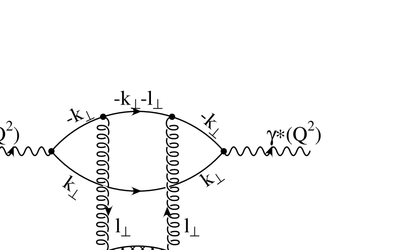
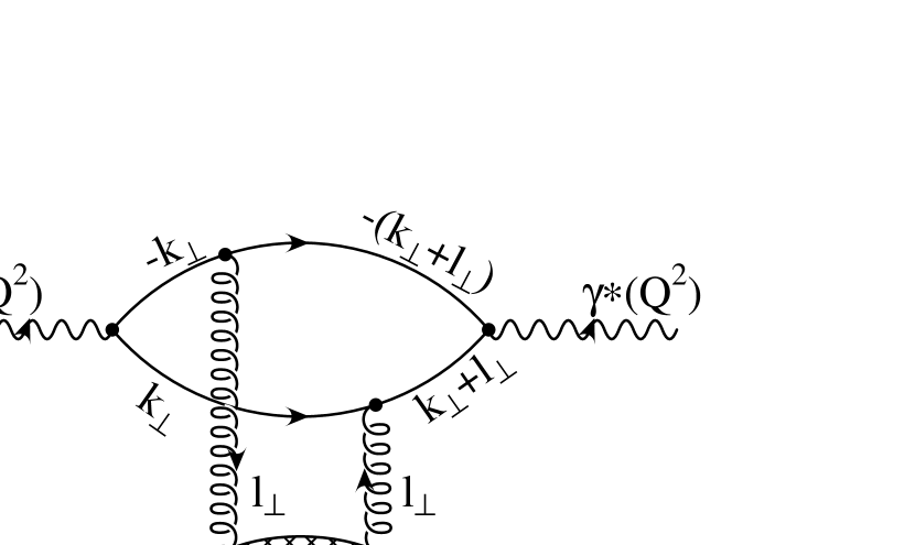
and, moreover, we noted that the scaling law (1.1) follows from the generalized vector dominance/colour-dipole picture (GVD/CDP). This picture of DIS at low $x$ rests [8] on $\gamma^{*}(q\bar{q})$ transitions, propagation of the $q\bar{q}$ state and its forward scattering from the proton via the generic structure of two-gluon exchange [9]. Accordingly, the GVD/CDP supplements the traditional (off-diagonal) GVD approach [2, 10] by taking into account the $q\bar{q}$ configuration in the $\gamma^{*}(q\bar{q})$ transition, as well as the generic structure of the two-gluon-exchange interaction, the $q\bar{q}$ colour dipole is subject to [11], when transversing the proton. The dimensionless low-$x$ scaling variable $\eta$ in (1.1) is given by $\eta(\Lambda^{2}(W^{2}),Q^{2})=(Q^{2}+m_{0}^{2})/\Lambda^{2}(W^{2})$, where $\Lambda^{2}(W^{2})$ is an increasing function of $W^{2}$ and $m_{0}^{2}$ denotes a threshold mass.

In the present paper, we provide a detailed account of our recent findings. In Section 2, we will give an explicit analytic representation of $\sigma_{\gamma^{*}p}(W^{2},Q^{2})$ in the GVD/CDP. We will derive the scaling law (1.1), and we will discuss the photoproduction limit and the relation of the present approach to the pre-QCD formulation of off-diagonal GVD. In Section 3, we will present the model-independent analysis of the experimental data that establishes the empirical validity of the scaling law (1.1). Subsequently, we will show that the observed $\eta$ dependence of the data coincides with the one predicted by the GVD/CDP. Final conclusions will be given in Section 4.

2 The generalized vector dominance/colour-dipole picture (GVD/CDP).

2.1 Generalities

We follow custom [12, 13] and as a starting point adopt a representation of the virtual-photon-proton cross section, $\sigma_{\gamma^{*}_{T,L}p}(W^{2},Q^{2})$, in transverse position space. Subsequently, we transform to momentum space, rather than proceeding in historical order [11, 8] from momentum space to transverse position space.

In transverse position space, accordingly, we represent $\sigma_{\gamma^{*}_{T,L}p}(W^{2},Q^{2})$ as an integral over the variables $\vec{r}_{\perp}$ and $z$ determining the $(q\bar{q})$ configuration in the $\gamma^{*}(q\bar{q})$ transition [8],

$$\sigma_{\gamma^{*}_{T,L}p}(W^{2},Q^{2})=\sum_{\lambda,\lambda^{\prime}=\pm 1}\int dz\int d^{2}r_{\perp}|\psi^{(\lambda,\lambda^{\prime})}_{T,L}(\vec{r}_{\perp},z,Q^{2})|^{2}\sigma_{(q\bar{q})p}(\vec{r}^{~{}2}_{\perp},z,W^{2}).$$ (2.1)

The $\gamma^{*}(q\bar{q})$ transition amplitude, known as the photon wave function, for transverse $(T)$ and longitudinal $(L)$ photons is described by $\psi^{(\lambda,\lambda^{\prime})}_{T,L}(r_{\perp},z,Q^{2})$. Implicitly, (2.1) contains the assumption that the configuration variable $z$ remains unchanged during the $(q\bar{q})p$ scattering process. The representation (2.1) must be read in conjunction with [8]

$$\sigma_{(q\bar{q})p}(\vec{r}^{~{}2}_{\perp},z,W^{2})=\int d^{2}l_{\perp}\tilde{\sigma}_{(q\bar{q})p}(\vec{l}^{~{}2}_{\perp},z,W^{2})(1-e^{-i\vec{l}_{\perp}\cdot\vec{r}_{\perp}}),$$ (2.2)

that implies

$$\sigma_{(q\bar{q})p}(\vec{r}^{~{}2}_{\perp},z,W^{2})\to\left\{\begin{array}[]{c@{\quad, \quad}l}\vec{r}^{~{}2}_{\perp}\cdot\frac{\pi}{4}\int d\vec{l}^{~{}2}_{\perp}\cdot\vec{l}^{~{}2}_{\perp}\ \tilde{\sigma}_{(q\bar{q})p}(\vec{l}^{~{}2}_{\perp},z,W^{2})&{\rm for}~{}r_{\perp}\to 0,\\ \int d^{2}l_{\perp}\tilde{\sigma}_{(q\bar{q})p}(\vec{l}^{~{}2}_{\perp},z,W^{2})&{\rm for}~{}r_{\perp}\to\infty.\end{array}\right.$$ (2.3)

The two-dimensional vector $\vec{l}_{\perp}$ is to be identified with the transverse (gluon) momentum absorbed or emitted by the quark (compare fig.1). The vanishing of the colour-dipole cross section, $\sigma_{(q\bar{q})p}(\vec{r}^{~{}2}_{\perp},z,W^{2})$, for vanishing transverse interquark separation is known as “colour transparency” [11].

The generic two-gluon-exchange structure (compare fig.1) contained in (2.2) becomes explicit when inserting (2.2) into (2.1) in conjunction with the Fourier representation of the photon wave function,

$$\psi^{(\lambda,\lambda^{\prime})}_{T,L}(\vec{r}_{\perp},z,Q^{2})={{\sqrt{4\pi}}\over{16\pi^{3}}}\int_{k_{\perp 0}}d^{2}k_{\perp}exp(i\vec{k}_{\perp}\cdot\vec{r}_{\perp}){\cal M}^{(\lambda,\lambda^{\prime})}_{T,L}(\vec{k}_{\perp},z;Q^{2}).$$ (2.4)

One obtains (cf. [8])

$$\sigma_{\gamma^{*}_{T,L}p}(W^{2},Q^{2})$$

$$={N_{c}\over{16\pi^{3}}}\sum_{\lambda,\lambda^{\prime}=\pm 1}\int dz\int d^{2}l_{\perp}\tilde{\sigma}_{(q\bar{q})p}(\vec{l}^{~{}2}_{\perp},z,W^{2})$$

$$\times \int_{|\vec{k}_{\perp}|\geq k_{\perp 0}}d^{2}k_{\perp}\int_{|\vec{k}^{~{}\prime}_{\perp}|\geq k_{\perp 0}}d^{2}k^{\prime}_{\perp}$$

$$\times {\cal M}^{(\lambda,\lambda^{\prime})}_{T,L}(\vec{k}^{\prime}_{\perp},z;Q^{2})^{*}{\cal M}^{(\lambda,\lambda^{\prime})}_{T,L}(\vec{k}_{\perp},z;Q^{2})$$

$$\times \left[\delta(\vec{k}^{\prime}_{\perp}-\vec{k}_{\perp})-\delta(\vec{k}^{\prime}_{\perp}-\vec{k}_{\perp}-\vec{l}_{\perp})\right],$$ (2.5)

where $N_{c}=3$ denotes the number of quark colours. The amplitudes ${\cal M}_{T,L}^{(\lambda,\lambda^{\prime})}(\vec{k}_{\perp},z;Q^{2})$ in (2.4) and (2.1) contain [8] the couplings of the photon to the $q\bar{q}$ pair as well as the propagators of the $q\bar{q}$ pair of mass $M_{q\bar{q}}$, where in terms of the quark (antiquark) transverse momentum, $|\vec{k}_{\perp}|$,

$$M^{2}_{q\bar{q}}={{\vec{k}^{~{}2}_{\perp}}\over{z(1-z)}}.$$ (2.6)

Transitions diagonal and off-diagonal in the masses of the initial and final $q\bar{q}$ states, $M_{q\bar{q}}$ from (2.6), and $M^{\prime}_{q\bar{q}}$ according to

$$M^{\prime 2}_{q\bar{q}}={{(\vec{k}_{\perp}+\vec{l}_{\perp})^{2}}\over{z(1-z)}},$$ (2.7)

contribute with equal weight to (2.1), but opposite in sign, as required by the generic two-gluon-exchange structure.

Conversely, it is precisely the generic two-gluon-exchange structure of the forward-virtual-Compton-scattering amplitude that justifies (2.1) as a starting point for low-x DIS.

According to (2.3), $\tilde{\sigma}_{(q\bar{q})p}(\vec{l}^{~{}2}_{\perp},z,W^{2})$ should vanish sufficiently rapidly to yield a convergent integral. It may be suggestive to assume a Gaussian in $\vec{l}^{~{}2}_{\perp}$ for $\tilde{\sigma}_{(q\bar{q})p}(\vec{l}^{~{}2}_{\perp},z,W^{2}).$ Actually, explicit calculations become much simpler if, without much loss of generality, instead of a Gaussian a $\delta$-function, located at a finite value of $\vec{l}^{~{}2}_{\perp}$, is used as an effective description of $\tilde{\sigma}_{(q\bar{q}p)}(\vec{l}^{~{}2}_{\perp},z,W^{2})$.

Accordingly, we adopt the simple ansatz[7],

$$\tilde{\sigma}_{(q\bar{q}p)}(\vec{l}^{~{}2}_{\perp},z,W^{2})=\sigma^{(\infty)}(W^{2}){1\over\pi}\delta(\vec{l}^{~{}2}_{\perp}-z(1-z)\Lambda^{2}(W^{2})).$$ (2.8)

This ansatz associates with any given energy, $W$, an (effective) fixed value of the two-dimensional (gluon) momentum transfer, $|\vec{l}_{\perp}|$, determined by the so far unspecified function $\Lambda(W^{2})$. The ansatz (2.8) also incorporates the assumption that ‘aligned’, $z\to 0$, configurations[14] of the $q\bar{q}$ pair absorb vanishing, $\vec{l}^{~{}2}_{\perp}\to 0$, gluon momentum.

For the subsequent interpretation of our results, we note the explicit form of the transverse-position-space colour-dipole cross section, obtained by substituting (2.8) into (2.2),

$$\sigma_{(q\bar{q})p}(\vec{r}^{~{}2}_{\perp},z,W^{2})=\sigma^{(\infty)}(W^{2})(1-J_{0}(r_{\perp}\cdot\sqrt{z(1-z)}\Lambda(W^{2})))$$

$$\simeq \sigma^{(\infty)}(W^{2})\cdot\left\{\begin{array}[]{l@{\quad~\quad}l}{1\over 4}z(1-z)\Lambda^{2}(W^{2})\vec{r}^{~{}2}_{\perp},\hfil\quad~{}&{\rm for}~{}{1\over 4}z(1-z)\Lambda^{2}(W^{2})\vec{r}^{~{}2}_{\perp}\to 0,\\[8.53581pt] 1,\hfil\quad~{}&{\rm for}~{}{1\over 4}z(1-z)\Lambda^{2}(W^{2})\vec{r}^{~{}2}_{\perp}\to\infty.\end{array}\right.$$ (2.11)

The limit of $\sigma^{(\infty)}(W^{2})$ in the second line of the approximate equality in (2.1) stands for an oscillating behaviour with decreasing amplitudes of the Bessel function, $J_{0}(r_{\perp}\sqrt{z(1-z)}\Lambda(W^{2}))$, around $\sigma^{(\infty)}(W^{2})$, when its argument tends towards infinity. Apart from these oscillations, the behaviour of $\sigma_{(q\bar{q})p}(\vec{r}^{~{}2}_{\perp},z,W^{2})$ in (2.1) is identical to the one obtained, if the $\delta$-function in (2.8) were replaced by a Gaussian. Concerning the high-energy behaviour of $\sigma_{(q\bar{q})p}(\vec{r}^{~{}2}_{\perp},z,W^{2})$, we note that it is consistent with unitarity restrictions, provided a decent high-energy behaviour is imposed on $\sigma^{(\infty)}(W^{2})$.

The ansatz (2.8) is to be seen as an effective realization, without much loss of generality, of the underlying requirements of colour transparency, (2.2), (2.3), and hadronic unitarity for the colour-dipole cross section. The unitarity requirement enters via the aforementioned decent high-energy behaviour of $\sigma^{(\infty)}(W^{2})$.

With (2.8), the virtual-photon-proton cross section (2.5) may be simplified considerably (cf. [8] as well as Appendix A). The right-hand side becomes reduced to essentially the product of $\sigma^{(\infty)}(W^{2})$ from (2.8) with a dimensionless integral over the masses $dM^{2}\equiv dM^{2}_{q\bar{q}}$ and $dM^{\prime 2}\equiv dM^{\prime 2}_{q\bar{q}}$ from (2.6) and (2.7). The dimensionless integral depends on the ratios of the available parameters, namely $Q^{2}/\Lambda^{2}(W^{2})$ and $m^{2}_{0}/\Lambda^{2}(W^{2})$, where $m^{2}_{0}$ stems from the lower limit of the integral in (2.1), where $k^{2}_{\perp 0}=z(1-z)m^{2}_{0}$. This threshold mass corresponds to the fact that the masses of hadronic vector states lie above a flavour-dependent lower limit. For non-strange quarks, we have $m^{2}_{0}\raise 1.29167pt\hbox{$<$\kern-7.5pt\raise-4.73611pt\hbox{$\sim$}}m^{2}_{\rho}$, i.e. $m^{2}_{0}$ is identified as the mass scale at which $e^{+}e^{-}\to~{}{\rm hadrons}$ reaches appreciable strength.

Instead of $Q^{2}/\Lambda^{2}(W^{2})$ and $m^{2}_{0}/\Lambda^{2}(W^{2})$, it will turn out to be preferable to use the low-x scaling variable[7]

$$\eta\Big{(}\Lambda^{2}(W^{2}),Q^{2}\Big{)}={{Q^{2}+m^{2}_{0}}\over{\Lambda^{2}(W^{2})}}$$ (2.12)

in conjunction with $m^{2}_{0}/\Lambda^{2}(W^{2})$. The virtual-photon-proton cross section (2.1) then becomes (compare Appendix A)

$$\sigma_{\gamma^{*}_{T,L}p}(W^{2},Q^{2})={{\alpha R_{e^{+}e^{-}}}\over{3\pi}}\sigma^{(\infty)}(W^{2})I_{T,L}(\eta,{{m^{2}_{0}}\over{\Lambda^{2}(W^{2})}}).$$ (2.13)

The quark charges $Q_{i}$ in units of the positron charge enter (2.13) via

$$R_{e^{+}e^{-}}=3\sum Q^{2}_{i},$$ (2.14)

that is the ratio of hadron production to $\mu^{+}\mu^{-}$ pair production in $e^{+}e^{-}$ annihilation. When specifying (2.13) to photoproduction, $Q^{2}=0$, only the light quark flavours ($u,\ d,\ s$) contribute appreciably, and, accordingly, $R_{e^{+}e^{-}}=2$ is to be inserted.

The function $I_{T,L}(\eta,m^{2}_{0}/\Lambda^{2}(W^{2}))$ in (2.13) is conveniently split into two additive contributions, a dominant term, $I^{(1)}_{T,L}$, and a correction term, $I_{T,L}^{(2)}$. This splitting will allow us to derive exact analytical expressions for one of the terms, the dominant one, while for the correction term, we will be content with an approximation in analytical form.

The integral representations for the transverse and longitudinal dominant parts, $I^{(1)}_{T}$ and $I^{(1)}_{L}$ read,

$$I^{(1)}_{T}\left(\eta,{{m^{2}_{0}}\over{\Lambda^{2}(W^{2})}}\right) ={1\over\pi}\int^{\infty}_{m^{2}_{0}}dM^{2}\int^{(M+\Lambda(W^{2}))^{2}}_{(M-\Lambda(W^{2}))^{2}}dM^{\prime 2}\omega(M^{2},M^{\prime 2},\Lambda^{2}(W^{2}))$$ (2.15)

$$\times\left[\frac{M^{2}}{(Q^{2}+M^{2})^{2}}-\frac{M^{\prime 2}+M^{2}-\Lambda^{2}(W^{2})}{2(Q^{2}+M^{2})(Q^{2}+M^{\prime 2})}\right],$$

and

$$I^{(1)}_{L}\left(\eta,{{m^{2}_{0}}\over{\Lambda^{2}(W^{2})}}\right) ={1\over\pi}\int^{\infty}_{m^{2}_{0}}dM^{2}\int^{(M+\Lambda(W^{2}))^{2}}_{(M-\Lambda(W^{2}))^{2}}dM^{\prime 2}\omega(M^{2},M^{\prime 2},\Lambda^{2}(W^{2}))$$ (2.16)

$$\times\left[\frac{Q^{2}}{(Q^{2}+M^{2})^{2}}-\frac{Q^{2}}{(Q^{2}+M^{2})(Q^{2}+M^{\prime 2})}\right].$$

The correction terms take the form

$$I^{(2)}_{T}\left(\eta,{{m^{2}_{0}}\over{\Lambda^{2}(W^{2})}}\right) ={1\over\pi}\int^{\infty}_{m^{2}_{0}}dM^{2}\Theta\left(m^{2}_{0}-(M-\Lambda(W^{2}))^{2}\right)\int^{m^{2}_{0}}_{(M-\Lambda(W^{2}))^{2}}dM^{\prime 2}$$ (2.17)

$$\times\omega(M^{2},M^{\prime 2},\Lambda^{2}(W^{2})){{M^{\prime 2}+M^{2}-\Lambda^{2}(W^{2})}\over{2(Q^{2}+M^{2})(Q^{2}+M^{\prime 2})}},$$

and

$$I^{(2)}_{L}\left(\eta,{{m^{2}_{0}}\over{\Lambda^{2}(W^{2})}}\right) ={1\over\pi}\int^{\infty}_{m^{2}_{0}}dM^{2}\Theta\left(m^{2}_{0}-(M-\Lambda(W^{2}))^{2}\right)\int^{m^{2}_{0}}_{(M-\Lambda(W^{2}))^{2}}dM^{\prime 2}$$ (2.18)

$$\times\omega(M^{2},M^{\prime 2},\Lambda^{2}(W^{2})){{Q^{2}}\over{(Q^{2}+M^{2})(Q^{2}+M^{\prime 2})}}.$$

Replacing the $\Theta$ function in (2.17) and in (2.18) by the integration limits in the integration over $dM^{2}$, we have

$$\int^{\infty}_{m^{2}_{0}}dM^{2}\Theta\left(m^{2}_{0}-(M-\Lambda(W^{2}))^{2}\right)\int^{m^{2}_{0}}_{(M-\Lambda(W^{2}))^{2}}dM^{\prime 2}...$$

$$=\left\{\begin{array}[]{ll}\int^{(m_{0}+\Lambda(W^{2}))^{2}}_{m_{0}^{2}}dM^{2}\int^{m_{0}^{2}}_{(M-\Lambda(W^{2}))^{2}}dM^{\prime 2}...&\mbox{, for }\Lambda(W^{2})<2m_{0},\\[8.53581pt] \int^{(\Lambda(W^{2})+m_{0})^{2}}_{(\Lambda(W^{2})-m_{0})^{2}}dM^{2}\int^{m_{0}^{2}}_{(M-\Lambda(W^{2}))^{2}}dM^{\prime 2}...&\mbox{, for }\Lambda(W^{2})>2m_{0},\end{array}\right.$$

i.e. the terms (2.17) and (2.18), when added to the dominant terms (2.15) and (2.16), respectively, assure that the lower limit of the integration over $dM^{\prime 2}$ is given by $M^{\prime 2}=m_{0}^{2}$, and coincides with the lower limit of the integration over $dM^{2}$, as required by symmetry in the incoming and outgoing $q\bar{q}$ masses. Actually it turns out that the transverse correction term, $I^{(2)}_{T}$, is negligible, while the longitudinal one is of some importance.

For the explicit expression for the integration measure $\omega(M^{2},M^{\prime 2},\Lambda^{2}(W^{2}))$ appearing in (2.15) to (2.18) we refer to Appendix A. For convenient reference, we note the integral relations [8]

$${1\over\pi}\int^{(M+\Lambda(W^{2}))^{2}}_{(M-\Lambda(W^{2}))^{2}}dM^{\prime 2}\omega(M^{2},M^{\prime 2},\Lambda^{2}(W^{2}))=1,$$ (2.22)

and

$${1\over\pi}\int^{(M+\Lambda(W^{2}))^{2}}_{(M-\Lambda(W^{2}))^{2}}dM^{\prime 2}\omega(M^{2},M^{\prime 2},\Lambda^{2}(W^{2}))M^{\prime 2}=M^{2}+\Lambda^{2}(W^{2}),$$ (2.23)

however.

2.2 Analytic evaluation of $\sigma_{\gamma^{*}p}(W^{2},Q^{2})$

We concentrate on the unpolarized cross section,

$$\sigma_{\gamma^{*}p}(W^{2},Q^{2})=\sigma_{\gamma^{*}_{T}p}+\sigma_{\gamma^{*}_{L}p},$$ (2.24)

and refer to Appendix B for a separate treatment of the longitudinal and transverse parts.

In terms of the sums of the transverse and longitudinal contributions in (2.15) and (2.16),

$$I^{(1)}=I^{(1)}_{T}+I^{(1)}_{L},$$ (2.25)

and in (2.17) and (2.18),

$$I^{(2)}=I^{(2)}_{T}+I^{(2)}_{L},$$ (2.26)

and upon taking the sum of the dominant and the correction part,

$$I\left(\eta,{{m^{2}_{0}}\over{\Lambda^{2}(W^{2})}}\right)=I^{(1)}\cdot\left(1+{{I^{(2)}}\over{I^{(1)}}}\right),$$ (2.27)

with (2.13), the unpolarized cross section (2.24) becomes

$$\sigma_{\gamma^{*}p}(W^{2},Q^{2})={{\alpha R_{e^{+}e^{-}}}\over{3\pi}}\sigma^{(\infty)}(W^{2})I\left(\eta,{{m^{2}_{0}}\over{\Lambda^{2}(W^{2})}}\right).$$ (2.28)

As mentioned, the integral representations for the dominant transverse and longitudinal contributions (2.15) and (2.16) may be analytically evaluated in a straight-forward manner. Accordingly, $I^{(1)}$ in (2.25) and (2.27) is explicitly given by

$$I^{(1)}\left(\eta,\mu\equiv\frac{m_{0}^{2}}{\Lambda^{2}(W^{2})}\right)$$

$$=\frac{1}{2} \ln\frac{\eta-1+\sqrt{(1+\eta)^{2}-4\mu}}{2\eta}$$

$$+\frac{1}{2\sqrt{1+4(\eta-\mu)}}\times \ln\frac{\eta\left(1+\sqrt{1+4(\eta-\mu)}\right)}{4\mu-1-3\eta+\sqrt{\Big{(}1+4(\eta-\mu)\Big{)}\Big{(}(1+\eta)^{2}-4\mu\Big{)}}}.$$ (2.29)

The correction term $I^{(2)}$ in (2.26), containing the sum of the integrals in (2.17) and (2.18), was evaluated by numerical integration for various sets of values of $\eta$ and $\mu$. Guided by these numerical results, we found a simple analytic approximation formula for the ratio in (2.27) that reads

$$1+\frac{I^{(2)}}{I^{(1)}}=1+2\frac{m_{0}^{2}}{\Lambda^{2}}\sqrt{\frac{1}{2}+\frac{1}{\pi}{\rm arctg}\left(\frac{1}{\pi}\left(\eta-\frac{m_{0}^{2}}{\Lambda^{2}}\right)-\frac{1}{2\left(\eta-\frac{m_{0}^{2}}{\Lambda^{2}}\right)}\right)}.$$ (2.30)

A comparison of the results of the numerical integration and the results of the analytic approximation (2.30) is shown in fig.2. In the range of the parameters $\eta$ and $m_{0}^{2}/\Lambda^{2}(W^{2})$ relevant in connection with the experimental data (compare Section 3), the error induced by employing the approximation formula (2.30) in (2.27) and (2.28) is less than 0.3 %. Accordingly, the expression (2.28) for $\sigma_{\gamma^{*}p}(W^{2},Q^{2})$ together with (2.27) and the analytical results (2.2) and (2.30) will form the basis for the analysis of the experimental data.

We briefly discuss the function $I(\eta,m^{2}_{0}/\Lambda^{2}(W^{2}))$, in (2.27) and (2.28) for various limits of the parameter space that will be relevant for the data analysis. First of all, for small values of $m^{2}_{0}/\Lambda^{2}(W^{2})$, one may expand the expression for $I^{(1)}(\eta,m^{2}_{0}/\Lambda^{2}(W^{2}))$ in (2.2) to yield

$$I^{(1)}\left(\eta,\frac{m_{0}^{2}}{\Lambda^{2}(W^{2})}\right)={\cal I}_{0}(\eta)+{\cal I}_{1}(\eta){{m^{2}_{0}}\over{\Lambda^{2}(W^{2})}}+{\rm O}\left({{m^{4}_{0}}\over{\Lambda^{4}(W^{2})}}\right),$$ (2.31)

where

$${\cal I}_{0}(\eta) = \frac{1}{2\sqrt{1+4\eta}}\ln\frac{\eta(1+\sqrt{1+4\eta})}{-1-3\eta+(1+\eta)\sqrt{1+4\eta}},$$

$${\cal I}_{1}(\eta) = \frac{1}{1+4\eta}\left(\frac{-3}{1+\eta}+2{\cal I}_{0}(\eta)\right).$$ (2.32)

A numerical evaluation shows that the term linear in $m^{2}_{0}/\Lambda^{2}(W^{2})$ becomes negligible as long as $m^{2}_{0}/\Lambda^{2}(W^{2})\raise 1.29167pt\hbox{$<$\kern-7.5pt\raise-4.73611pt\hbox{$\sim$}}1$. For $m^{2}_{0}/\Lambda^{2}(W^{2})<1$, also the correction term (2.30) does not deviate much from unity, and accordingly, $I(\eta,m^{2}_{0}/\Lambda^{2}(W^{2}))$ in (2.28), in good approximation, only depends on $\eta$,

$$I(\eta,m^{2}_{0}/\Lambda^{2}(W^{2}))\simeq{\cal I}_{0}(\eta).$$ (2.33)

For a sufficiently smooth $W$ dependence of $\sigma^{(\infty)}(W^{2})$ in (2.28), we have approximate scaling of the virtual-photon proton cross section,

$$\sigma_{\gamma^{*}p}(W^{2},Q^{2})\cong{{\alpha R_{e^{+}e^{-}}}\over{3\pi}}\sigma^{(\infty)}(W^{2}){\cal I}_{0}(\eta),$$ (2.34)

i.e. in good approximation, the $\gamma^{*}p$ total cross section only depends on the scaling variable $\eta=(Q^{2}+m_{0})/\Lambda^{2}(W^{2})$.

It is instructive to consider the limiting cases of small $\eta$ and large $\eta$ in ${\cal I}_{0}(\eta)$. From (2.2), one finds

$${\cal I}_{0}(\eta)=\left\{\begin{array}[]{ll}\ln(1/\eta)+{\rm O}(\eta\ln\eta),&\mbox{for }\eta\to\eta_{min}=m_{0}^{2}/\Lambda^{2}(W^{2}),\\[5.69054pt] 1/(2\eta)+{\rm O}(1/\eta^{2}),&\mbox{for }\eta\to\infty.\end{array}\right.$$ (2.35)

The behaviour of $\sigma_{\gamma^{*}p}(\eta)$ thus changes dramatically, from a logarithmic one for small $\eta$ to a powerlike one for large $\eta$. Note that the small-$\eta$ limit besides photoproduction $(Q^{2}=0)$ also includes the limit of fixed $Q^{2}$, but $\Lambda^{2}(W^{2})$ sufficiently large. As $\Lambda^{2}(W^{2})$ will turn out to increase as a power of $W^{2}$, one will be led to the conclusion that at any value of $Q^{2}$ the virtual-photon-proton cross section will at sufficiently high energy, that is for small $\eta$, exhibit the same smooth energy dependence that is observed in photoproduction.

2.3 The photoproduction limit and the significance of $\sigma^{(\infty)}(W^{2})$.

Evaluating the unpolarized cross section $\sigma_{\gamma^{*}p}(W^{2},Q^{2})$ in (2.28) for $Q^{2}=0$, or, equivalently, the transverse cross section (2.13), we obtain our result for the cross section of photoproduction,

$$\sigma_{\gamma p}(W^{2})={{\alpha R_{e^{+}e^{-}}}\over{3\pi}}\sigma^{(\infty)}(W^{2})I\left(\eta(\Lambda^{2}(W^{2}),Q^{2}=0),{{m^{2}_{0}}\over{\Lambda^{2}(W^{2})}}\right),$$ (2.36)

where, according to (2.12),

$$\eta(\Lambda^{2}(W^{2}),Q^{2}=0)={{m^{2}_{0}}\over{\Lambda^{2}(W^{2})}},$$ (2.37)

and $R_{e^{+}e^{-}}=2$ is to be inserted. To proceed, it is suggestive to require duality between the generic two-gluon-exchange structure of the GVD/CDP contained in (2.36) and the Regge behaviour experimentally verified for photoproduction. This duality assumption is meant with respect to Pomeron exchange that dominates photoproduction in the high-energy limit. Accordingly, we require

$$\sigma_{\gamma p}(W^{2})^{Regge}={{\alpha R_{e^{+}e^{-}}}\over{3\pi}}\sigma^{(\infty)}(W^{2})I\left({{m^{2}_{0}}\over{\Lambda^{2}(W^{2})}},{{m^{2}_{0}}\over{\Lambda^{2}(W^{2})}}\right),$$ (2.38)

where the notation $\sigma_{\gamma p}(W^{2})^{Regge}$ explicitly displays the duality hypothesis mentioned above. Solving (2.38) for $\sigma^{(\infty)}(W^{2})$,

$$\sigma^{(\infty)}(W^{2})={{\sigma_{\gamma p}(W^{2})^{Regge}}\over{{{\alpha R_{e^{+}e^{-}}}\over{3\pi}}I\left({{m^{2}_{0}}\over{\Lambda^{2}(W^{2})}},{{m^{2}_{0}}\over{\Lambda^{2}(W^{2})}}\right)}},$$ (2.39)

allows us to express the virtual-photon-proton cross section (2.13) explicitly in terms of$\sigma_{\gamma p}(W^{2})^{Regge}$,

$$\sigma_{\gamma^{*}_{T,L}p}(W^{2},Q^{2})=\sigma_{\gamma p}(W^{2})^{Regge}{{I_{T,L}\left(\eta(\Lambda^{2}(W^{2}),Q^{2}),{{m^{2}_{0}}\over{\Lambda^{2}(W^{2})}}\right)}\over{I\left({{m^{2}_{0}}\over{\Lambda^{2}(W^{2})}},{{m^{2}_{0}}\over{\Lambda^{2}(W^{2})}}\right)}}.$$ (2.40)

Concerning the relation (2.39), it seems appropriate to remind ourselves of the meaning of $\sigma^{(\infty)}(W^{2})$. According to (2.1), $\sigma^{(\infty)}(W^{2})$ denotes the limiting behaviour of the colour-dipole cross section, $\sigma_{(q\bar{q})p}(\vec{r}^{~{}2}_{\perp},z,W^{2})$, both for $r_{\perp}\to\infty$ with $\Lambda^{2}(W^{2})$ fixed, and for $\Lambda^{2}(W^{2})\to\infty$ with $r_{\perp}$ fixed. The $W$ dependence of $\sigma^{(\infty)}(W^{2})$, as a consequence of the (logarithmic) increase with energy of the denominator in (2.39), in general will deviate from the one of $\sigma_{\gamma p}(W^{2})^{Regge}$. This is not unexpected; the energy dependence of the colour-dipole cross section a priori need not coincide with the energy dependence characteristic for ordinary hadron-hadron interactions.

In connection with the energy dependence and the conceptual meaning of $\sigma^{(\infty)}(W^{2})$, a brief discussion of the $\rho^{0},\omega,\phi$-dominance [15] approximation for the virtual-photon-proton and, in particular, the photoproduction cross section will be helpful. Returning to (2.13), and ignoring the off-diagonal transitions in (2.13), we approximate the integral (2.15) by its integrand to obtain

$$\sigma_{\gamma^{*}_{T}p}(W^{2},Q^{2})={{\alpha R_{e^{+}e^{-}}}\over{3\pi}}{{\Delta M^{2}_{\rho}}\over{M^{2}_{\rho}}}{{M^{4}_{\rho}}\over{(Q^{2}+M^{2}_{\rho})^{2}}}\sigma^{(\infty)}(W^{2}).$$ (2.41)

In (2.41), we made the simplifying assumption of flavour-independent equal masses, $M^{2}\equiv M^{2}_{\rho}$, and equal level spacings, $\Delta M^{2}\equiv\Delta M^{2}_{\rho}$, for the dominant vector mesons, $\rho^{0},\omega$ and $\phi$. Moreover, by assuming $R_{e^{+}e^{-}}=2$, we ignore more massive vector-meson flavours, such as $J/\psi$, etc. The connection of (2.41) with $\rho^{0},\omega,\phi$-dominance for (virtual-) photon-hadron interactions becomes explicit by introducing the photon-vector-meson coupling strengths via quark-hadron duality [16],

$${{\alpha R_{e^{+}e^{-}}}\over{3\pi}}{{\Delta M^{2}_{\rho}}\over{M^{2}_{\rho}}}=\sum_{V=\rho^{0},\omega,\phi}{{\alpha\pi}\over{\gamma^{2}_{V}}},$$ (2.42)

as well as the identification of $\sigma^{(\infty)}(W^{2})$ with the total cross section of vector-meson-proton scattering,

$$\sigma^{(\infty)}(W^{2})=\sigma_{Vp}(W^{2}).$$ (2.43)

As a consequence of the simplification of flavour independence, $\sigma_{Vp}(W^{2})$ denotes a weighted average of the $(\rho^{0}p),(\omega p)$ and $(\phi p)$ cross sections. As the $(\rho^{0}p)$ and $(\omega p)$ cross sections agree with each other, and the $\phi$ contribution is suppressed by the smaller coupling to the photon and by the smaller $(\phi p)$ cross section [2], the weighted average in (2.43) may approximately be identified with the $(\rho^{0}p)$ cross section,

$$\sigma^{(\infty)}(W^{2})\cong\sigma_{\rho p}(W^{2}).$$ (2.44)

The couplings in (2.42), by definition, denote the coupling strengths of the photon to the vector mesons, $V=\rho^{0},\omega,\phi$, as measured in $e^{+}e^{-}$ annihilation by the integrals over the corresponding vector-meson peaks,

$${{\alpha\pi}\over{\gamma^{2}_{V}}}={1\over{4\pi^{2}\alpha}}\sum_{F}\int\sigma_{e^{+}e^{-}\to V\to F}(s)ds,$$ (2.45)

or equivalently, by the vector-meson widths,

$$\Gamma_{V\to e^{+}e^{-}}={{\alpha^{2}M^{2}_{V}}\over{12(\gamma^{2}_{V}/4\pi)}}.$$ (2.46)

Upon inserting the quark-hadron-duality relation (2.42) and the hadronic vector-meson-proton cross section (2.44) into (2.41), we obtain the $\rho^{0},\omega,\phi$-dominance prediction for the transverse virtual-photon-proton cross section. It exhibits the well-known violent disagreement with experiment for $Q^{2}>0$, even though $\rho^{0},\omega,\phi$-dominance yields a reasonable approximation for photoproduction [3]. Dropping the above simplification of flavour independence, it reads [3]

$$\sigma_{\gamma p}(W^{2})=\sum_{V=\rho^{0},\omega,\phi}{{\alpha\pi}\over{\gamma^{2}_{V}}}\sigma_{Vp}(W^{2})={{\alpha\pi}\over{\gamma^{2}_{\rho}}}\sigma_{\rho p}\left(1+{1\over 9}+{2\over 9}\cdot{1\over 2}\right),$$ (2.47)

where the relative weight of the $w$ and $\phi$ contributions is determined by the quark content of their wave functions, and $\sigma_{\phi p}\cong(1/2)\sigma_{\rho p}$ is used. Numerically, from (2.46), by inserting $\Gamma_{V\to e^{+}e^{-}}\cong 6.5{\rm keV}$, one finds $\gamma^{2}_{\rho}/4\pi\cong 0.53$, and accordingly (2.47) yields

$$\sigma_{\gamma p}(W^{2})=(1/240)\sigma_{\rho p}(W^{2}).$$ (2.48)

This relation will be used in Section 3.3. It is of approximate validity. A careful analysis at energies around $W\cong 3{\rm GeV}$ revealed that the right-hand side in (2.48) yields 78 % of $\sigma_{\gamma p}$ [2].

Even though the above exposition of how the $\rho^{0},\omega,\phi$-dominance approximation is contained in the GVD/CDP may be useful in its own right, it has been our main concern in this section to illuminate the meaning of $\sigma^{(\infty)}(W^{2})$. In general, $\sigma^{(\infty)}(W^{2})$ in (2.39) differs conceptually, and in its energy dependence, from a vector-meson-proton cross section. It is in the $\rho^{0},\omega,\phi$-dominance approximation (2.41) that an identification of $\sigma^{(\infty)}(W^{2})$ with the hadronic cross section, $\sigma_{\rho p}(W^{2})$ in (2.44), becomes justified. A strict validity of (2.44), however, when inserted into (2.36), requires $\Lambda^{2}(W^{2})$ to be an energy-independent constant. Such a requirement, in turn, implies the energy dependence of $\sigma_{\gamma^{*}p}(W^{2},Q^{2})$ to be identical for all $Q^{2}$, in gross disagreement with the experimental results from HERA [17, 18].

2.4 A reference to pre-QCD off-diagonal generalized vector dominance

As strongly emphasized before [8], and explicitly displayed in (2.1), in the GVD/CDP, it is the generic two-gluon-exchange structure of the $(q\bar{q})p$ interaction that leads to the characteristic difference in sign between, and the necessary cancellation of diagonal and off-diagonal contributions to the virtual-forward-Compton-scattering amplitude. The difference in sign corresponds to destructive interference between hadron-production amplitudes induced by different masses of the $q\bar{q}$ states the incoming photon dissociates into. The destructive interference is a necessity [10] for the convergence of the mass dispersion relations (2.15) to (2.18), or, in other words, the consistency of scaling in $e^{+}e^{-}$ annihilation into hadrons with the GVD picture of DIS at low x. Off-diagonal transitions in the mass dispersion relation, in order to simplify the formalism, were frequently ignored [2, 19] in the past, at the expense of introducing an ad hoc effective $1/M^{2}$ decrease of the $(q\bar{q})p$ strong-interaction cross section. This approximation is confronted with consistency problems [10], and an approach that does not rely on the diagonal approximation is preferable right from the outset.

The necessary cancellation in the virtual-forward-Compton amplitude between diagonal and off-diagonal transitions was anticipated [10] during the pre-QCD era. We indicate how an approximate evaluation of the GVD/CDP indeed coincides with the pre-QCD formulation of off-diagonal GVD.

We concentrate on the transverse part of the virtual-photon-proton cross section in (2.13) and consider the off-diagonal term in the mass dispersion relation (2.15). In order to find an approximate evaluation of the off-diagonal contribution to the integral in (2.15), we start by tentatively putting $M^{\prime 2}=M^{2}$ in the denominator of (2.15). Under this assumption, the integration over $dM^{\prime 2}$ can be easily carried out by employing the integral relations for $\omega(M^{2},M^{\prime 2},\Lambda^{2}(W^{2}))$ in (2.22) and (2.23). One notes that the result of this integration is identically reproduced by replacing $M^{\prime 2}$ by $M^{\prime 2}=M^{2}+\Lambda^{2}(W^{2})$ in the multiplicative factor in front of $\omega(M^{2},M^{\prime 2},\Lambda^{2}(W^{2}))$ in (2.15) prior to integrating over $dM^{\prime 2}$. Returning to the correct off-diagonal term in (2.15) by dropping the simplifying assumption of $M^{\prime 2}=M^{2}$ in the denominator in (2.15), we now replace $M^{\prime 2}$ in the factor multiplying $\omega(M^{2},M^{\prime 2},\Lambda^{2}(W^{2}))$ by the more general mean value

$$M^{\prime 2}=M^{2}+{{\Lambda^{2}(W^{2})}\over{1+2\delta_{T}}},$$ (2.49)

that contains the parameter $\delta_{T}$. The parameter $\delta_{T}$ is to be chosen such that the off-diagonal integral is properly reproduced in the sense of a mean-value evaluation of this integral. With the substitution (2.49), as specified, and upon integration over $dM^{\prime 2}$, using (2.22), the integral (2.15) becomes

$$I_{T}\left(\eta,{{m^{2}_{0}}\over{\Lambda^{2}(W^{2})}}\right)\simeq\int^{\infty}_{m^{2}_{0}}dM^{2}\left[{{M^{2}}\over{(Q^{2}+M^{2})^{2}}}-{{M^{2}-\delta_{T}{{\Lambda^{2}(W^{2})}\over{1+2\delta_{T}}}}\over{(Q^{2}+M^{2})(Q^{2}+M^{2}+{{\Lambda^{2}(W^{2})}\over{1+2\delta_{T}}}}}\right].$$ (2.50)

With (2.50), and using the quark-hadron-duality relation (2.42), as well as the identification (2.44), the cross section resulting from (2.13),

$$\sigma_{\gamma^{*}_{T}p}(W^{2},Q^{2}) =\sum_{V=\rho^{0},\omega,\phi}{{\alpha\pi}\over{\gamma^{2}_{V}}}\sigma_{Vp}(W^{2}){{m^{2}_{\rho}}\over{\Delta m^{2}_{\rho}}}$$ (2.51)

$$\times\int^{\infty}_{m^{2}_{0}}dM^{2}\left[{{M^{2}}\over{(Q^{2}+M^{2})^{2}}}-{{M^{2}-\delta_{T}{{\Lambda^{2}(W^{2})}\over{1+2\delta_{T}}}}\over{(Q^{2}+M^{2})(Q^{2}+M^{2}+{{\Lambda^{2}(W^{2})}\over{1+2\delta_{T}}}}}\right],$$

coincides with the one in ref. [10] in the approximation that $\Lambda^{2}$ and $\delta_{T}$ are treated as appropriately chosen constants.

The original derivation [10] that led to (2.51) was based on an infinite series of discrete vector-meson states. The opposite signs of diagonal and off-diagonal transitions were located at the $\gamma^{*}(q\bar{q})$-transition vertices, as, e.g., had been suggested by bound-state quark-model calculations [21]. It is amusing to note that the anticipated structure, in the framework of QCD, now finds an entirely different justification: the origin of the sign difference has shifted from the $\gamma^{*}(q\bar{q})$ vertices to the generic structure of the two-gluon-exchange amplitude in the purely hadronic $(q\bar{q})p$ interaction.

3 The generalized vector dominance/colour-dipole picture confronting the experimental data on $\sigma_{\gamma^{*}p}(W^{2},Q^{2})$.

In confronting the theoretical results from Section 2 with the experimental data, we will follow the strategy employed in our recent communication [7]. In Section 3.1, accordingly, the prediction (2.34) of scaling for the $\gamma^{*}p$ total cross section,

$$\sigma_{\gamma^{*}p}(W^{2},Q^{2})\simeq\sigma_{\gamma^{*}p}(\eta)$$ (3.1)

will be tested in a model-independent approach. In Section 3.2, the empirical validity of the functional dependence of $\sigma_{\gamma^{*}p}(\eta)$ on $\eta$ in the GVD/CDP given in (2.27) to (2.30) will be investigated.

3.1 Low-$x$ scaling in $\gamma^{*}p$ total cross sections

The scaling variable $\eta$ was defined by (2.12) as the ratio of $Q^{2}+m^{2}_{0}$ over $\Lambda^{2}(W^{2})$. According to (2.8), $\Lambda(W^{2})$ determines the magnitude of the (two-dimensional) momentum transfer $|\vec{l}_{\bot}|$ to the quark and antiquark. As a consequence, $\Lambda(W^{2})$ also determines the magnitude of the final-state $q\bar{q}$ masses, $M^{\prime}$, that can be reached from a given $q\bar{q}$ mass, $M$, in the initial state. This interpretation suggests that $\Lambda^{2}(W^{2})$ be an increasing function of the energy, $W$. We will adopt a power-law ansatz,

$$\Lambda^{2}(W^{2})=C_{1}(W^{2}+W^{2}_{0})^{C_{2}},$$ (3.2)

and, alternatively, a logarithmic one,

$$\Lambda^{2}(W^{2})=C^{\prime}_{1}\ln\left(\frac{W^{2}}{W^{\prime 2}_{0}}+C^{\prime}_{2}\right).$$ (3.3)

Altogether, the scaling variable $\eta$ depends on $m^{2}_{0}$ and the constants $C_{1},W^{2}_{0},C_{2}$ (or, alternatively, $C^{\prime}_{1},W^{\prime 2}_{0},C^{\prime}_{2}$) to be determined by a fit to the data based on the scaling conjecture (3.1). In the model-independent test of scaling, no specific functional dependence of the total cross section (3.1) on $\eta$ is assumed. Accordingly, in the model-independent analysis, the parameter $C_{1}$ (or, alternatively, the parameter $C^{\prime}_{1}$) remains undetermined. A change of $C_{1}$ (or $C^{\prime}_{1}$) amounts to a rescaling of $\eta$ to $C^{-1}_{1}\eta$ (or $C^{\prime-1}_{1}\eta$), and, accordingly, the absolute value of $C_{1}$ (or $C^{\prime}_{1}$) is irrelevant for the existence of a scaling behaviour for the $\gamma^{*}p$ total cross section. For the analysis and the representation of the data, we will use a value of $C_{1}$ (or $C^{\prime}_{1}$) that coincides with, or is in the vicinity of the value to be determined in the fit to the data based on the GVD/CDP in Section 3.2.

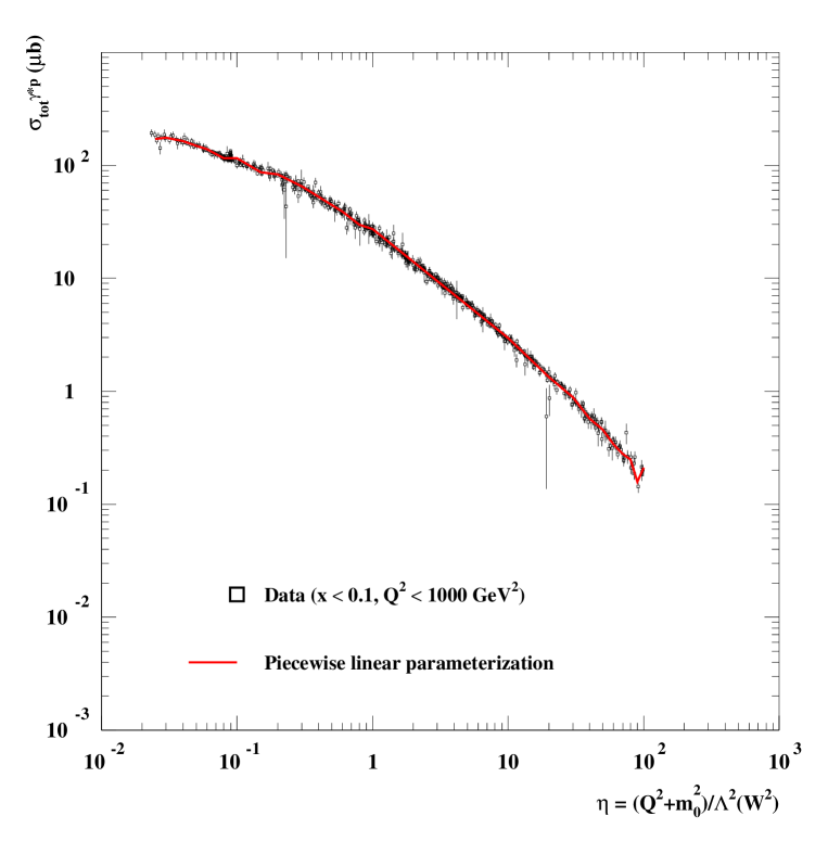
Technically, the empirical test of the scaling law (3.1) is carried out as follows. Without loss of generality, we assume that the conjectured scaling curve for $\sigma_{\gamma^{*}p}(\eta)$ may be represented by a piecewise linear function of $\eta$. This assumption allows us to perform a fit to the data that determines the parameters $m^{2}_{0},W^{2}_{0},C_{2}$ simultaneously with the values of the piecewise linear function $\sigma_{\gamma^{*}p}(\eta)$ at a number of points $\eta_{i}(i=1,...,N)$ of the variable $\eta$.

In fig.3, we show the result of the model-independent analysis. For $C_{1}(C^{\prime}_{1})$ the numerical value of $C_{1}=0.34$ ($C^{\prime}_{1}=1.64\ {\rm GeV}^{2}$) was chosen. As seen in fig.3, upon imposing the kinematic restriction of $x\leq 0.1$ and $Q^{2}\leq 1000{\rm GeV}^{2}$, all available experimental data [17, 18, 22, 23, 24] on photo- and electroproduction are indeed seen to lie on a smooth curve that, for technical reasons, is approximated by the piecewise linear fit function. The parameters obtained from the fit, using the power-law ansatz (3.2), are given by

$$m^{2}_{0} = 0.125\pm 0.027{\rm GeV}^{2},$$

$$C_{2} = 0.28\pm 0.06,$$ (3.4)

$$W^{2}_{0} = 439\pm 94{\rm GeV}^{2},$$

with $\chi^{2}$ per degree of freedom, $\chi^{2}$/ndf=1.15. For the logarithmic ansatz, we obtained

$$m^{2}_{0} = 0.12\pm 0.04{\rm GeV}^{2},$$

$$C^{\prime}_{2} = 3.5\pm 0.6,$$ (3.5)

$$W^{\prime 2}_{0} = 1535\pm 582{\rm GeV}^{2},$$

with $\chi^{2}$/ndf=1.18.

We note that an analogous procedure, applied to the experimental data without a restriction on $x$, does not lead to a universal curve. Likewise, restricting oneself to only those data points that belong to $x>0.1$, no universal curve is obtained either; the fitting procedure leads to entirely unacceptable results on the quality of the fit as quantified by the value of $\chi^{2}$ per degree of freedom.

The model-independent phenomenological analysis thus reveals that the scaling behaviour of the virtual-photon-proton cross section derived from the GVD/CDP is indeed borne out by the experimental data. This result by itself does not allow one to conclude that also the specific functional dependence on $\eta$ of the GVD/CDP, or on $W^{2}$ and $Q^{2}$ as given in Section 2.2, holds for the data on the $\gamma^{*}p$ total cross section. To investigate this question, we turn to Section 3.2.

3.2 Testing the $\eta$ dependence of $\sigma_{\gamma^{*}p}$ in the GVD/CDP

Upon replacing $\sigma^{(\infty)}(W^{2})$ in (2.28) by the Regge-parameterization of the total photoproduction cross section according to (2.39), we have

$$\sigma_{\gamma^{*}p}(W^{2},Q^{2})=\sigma_{\gamma p}(W^{2})^{Regge}\frac{I(\eta(\Lambda^{2}(W^{2}),Q^{2}),\frac{m^{2}_{0}}{\Lambda^{2}(W^{2})})}{I(\frac{m^{2}_{0}}{\Lambda^{2}(W^{2})},\frac{m^{2}_{0}}{\Lambda^{2}(W^{2})})}.$$ (3.6)

The analytical results for $I(\eta,\frac{m^{2}_{0}}{\Lambda^{2}(W^{2})})$ to be employed in the fits are given in (2.27) with (2.2) and (2.30). For $m_{0}^{2}/\Lambda^{2}(W^{2})\ll 1$, we have (approximate) scaling, compare (2.33) and (2.35).

In (3.6), for the photoproduction cross section, we use the parameterization

$$\sigma_{\gamma p}(W^{2})^{Regge}=A_{R}(W^{2})^{\alpha_{R}-1}+A_{P}(W^{2})^{\alpha_{P}-1},$$ (3.7)

where $W^{2}$ is to be inserted in units of $\rm GeV^{2}$ and [25]

$$A_{R} = 145.0\pm 2.0\;{\rm\mu b},$$

$$\alpha_{R} = 0.5,$$ (3.8)

$$A_{P} = 63.5\pm 0.9\;{\rm\mu b},$$

$$\alpha_{P} = 1.097\pm 0.002.$$

For a test of the empirical validity of the GVD/CDP formula (3.6), one may evaluate (3.6) for the power-law ansatz for $\Lambda^{2}(W^{2})$ in (3.2), or the logarithmic one in (3.3), using the parameters (3.1) and (3.1) from the model-independent fit, and determine $C_{1}(C_{1}^{\prime})$ by a fit of (3.6) to the experimental data for $\sigma_{\gamma^{*}p}(W^{2},Q^{2})$.

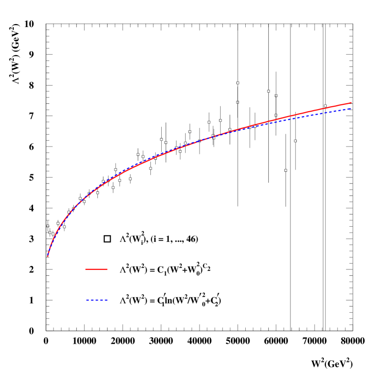
The alternative approach, actually employed in our analysis, is as follows. Rather than relying on the functional form of, and the values of the parameters in $\Lambda^{2}(W^{2})$ from the model-independent analysis, we only assume that $\Lambda^{2}(W^{2})$ can be described by a smooth piecewise linear function of $W^{2}$. The fit of (3.6) to the data for $\sigma_{\gamma^{*}p}(W^{2},Q^{2})$ then is to determine $m_{0}^{2}$, as well as the values of $\Lambda^{2}(W^{2})$ at a set of chosen values, $W^{2}_{i}$, for $i=1,{\ldots},N$. The values of $\Lambda^{2}(W^{2}_{i})$ obtained in our fit (for $i=1,{\ldots},46$) under the restriction of $x\leq 0.01$ and $Q^{2}\leq 100GeV^{2}$ are shown in fig.4. This fitting procedure, with an acceptable $\chi^{2}/ndf=1.15$, provides the most direct empirical verification of the $Q^{2}$ dependence of the GVD/CDP. At any energy, $W_{i}$, the $Q^{2}$ dependence, by our fit, is indeed verified to be described by (2.15) to (2.18), or rather (2.2) and (2.30), upon inserting the appropriate value of $\Lambda^{2}(W^{2}_{i})$ from fig.4.

It is in a second step that we now assume the powerlike and the logarithmic analytical form, respectively, for $\Lambda^{2}(W^{2})$ in (3.2) and (3.3), in order to fit (3.6) to the experimental data for the $\gamma^{*}p$ interaction again. The resulting curves for $\Lambda^{2}(W^{2})$ are also displayed in fig.4, and are seen to provide a good representation of the results for $\Lambda^{2}(W^{2}_{i})$. The fit parameters, in distinction to (3.1) and (3.1), now include the absolute normalization $C_{1}$ $(C_{1}^{\prime})$ of the scaling variable $\eta$. The fitted parameters are given by

$$m_{0}^{2} = 0.16\pm 0.01\;{\rm GeV^{2}},$$

$$C_{1} = 0.34\pm 0.05,$$ (3.9)

$$C_{2} = 0.27\pm 0.01,$$

$$W_{0}^{2} = 882\pm 246\;{\rm GeV^{2}},$$

with $\chi^{2}/ndf=1.15$ for the power-law ansatz, and by

$$m_{0}^{2} = 0.157\pm 0.009\;{\rm GeV^{2}},$$

$$C_{1}^{\prime} = 1.64\pm 0.14{\rm GeV^{2}},$$ (3.10)

$$C_{2}^{\prime} = 4.1\pm 0.4,$$

$${W^{\prime}}^{2}_{0} = 1015\pm 334\;{\rm GeV^{2}},$$

with $\chi^{2}/ndf=1.19$ for the logarithmic one. Since both, the model-independent fit and the one based on the GVD/CDP, describe the experimental data, the parameters in $\eta\Big{(}\Lambda^{2}(W^{2}),Q^{2}\Big{)}$ resulting from the different fit procedures must be consistent with each other. This is the case, compare (3.2) and (3.2) with (3.1) and (3.1), respectively.

It is worth stressing at this point that $\Lambda^{2}(W^{2})$, shown in fig.4, not only yields the denominator of the scaling variable $\eta$. According to (2.1), $\Lambda^{2}(W^{2})$ directly determines the energy dependence of the colour-dipole cross section in the limit of $\Lambda^{2}(W^{2})\vec{r}^{~{}2}_{\perp}\to 0$, that is the limit of sufficiently small interquark separation in the colour dipole and for non-asymptotic energies.

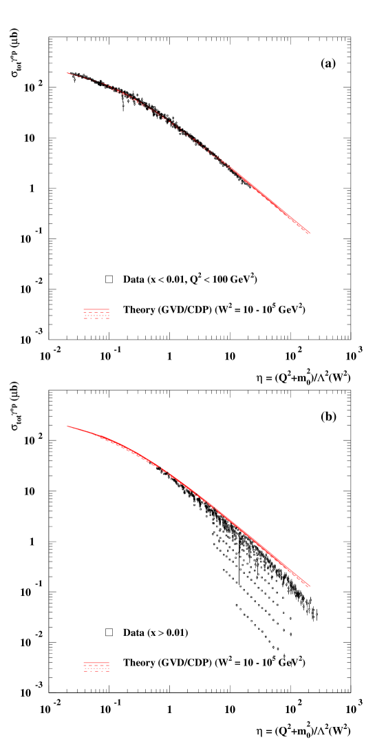
In fig.5, we show the explicit comparison of the experimental data for $\sigma_{\gamma^{*}p}(W^{2},Q^{2})$ as a function of $\eta$ with the theoretical results of the GVD/CDP. The (approximate) coincidence of the theoretical predictions over a wide range of $W^{2}$, from $W^{2}\approx 10\mbox{GeV}^{2}$ to $W^{2}\approx 10^{5}\mbox{GeV}^{2}$, demonstrates the scaling property of the theory. As shown in fig.5a, with the restrictions $x<0.01$ and $Q^{2}<100GeV^{2}$ imposed on the data (as in the above fit), there is good agreement between theory and experiment. In fig.5b, we show the deviations between theory and experiment, occurring when data for $x\geq 0.01$ are taken into account exclusively.

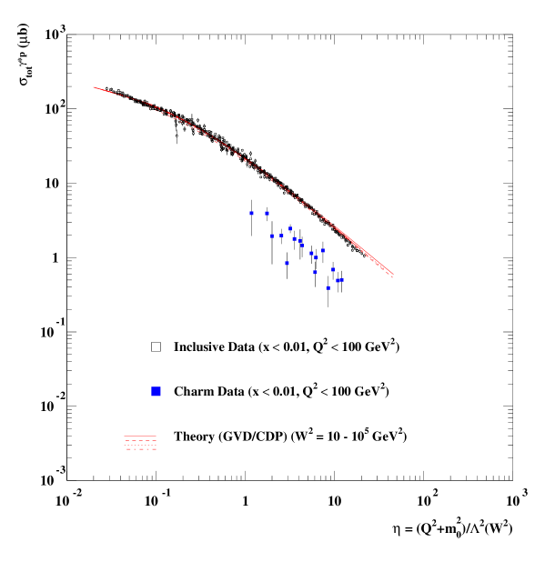
One may wonder about the influence of the charm contribution on the total cross section with respect to the scaling behaviour in $\eta$. A priori, one may expect charm production, when analysed by itself, to lead to a different mass scale, $m^{2}_{charm}>m^{2}_{0}$, in $\eta$. In fig.6, we have plotted the experimental data [26] for $\sigma_{\gamma^{*}p}^{charm}(W^{2},Q^{2})$ against $\eta$, in addition to the total cross section, $\sigma_{\gamma^{*}p}(W^{2},Q^{2})$. The charm-production data contribute roughly 30 % to $\sigma_{\gamma^{*}p}(\eta)$, but otherwise show approximately the same dependence on $\eta$ as observed for $\sigma_{\gamma^{*}p}(\eta)$. Note that for the charm data, $Q^{2}\raise 1.29167pt\hbox{$>$\kern-7.5pt\raise-4.73611pt\hbox{$\sim$}}10\mbox{GeV}^{2}$, such that it is fairly irrelevant whether $\eta=(Q^{2}+m_{0}^{2})/\Lambda^{2}(W^{2})$ or $\eta=(Q^{2}+m_{charm}^{2})/\Lambda^{2}(W^{2})$ is used as a scaling variable. Clearly, if precise data on charm production will be analysed with respect to their scaling properties, one expects to arrive at $m^{2}_{charm}$ replacing $m_{0}^{2}$ in $\eta$. This is irrelevant for the total cross section, however, since with smaller values of $Q^{2}$, charm production soon becomes a minor contribution to $\sigma_{\gamma^{*}p}(W^{2},Q^{2})$.

As noted, the theoretical prediction (3.6) is based on the replacement of the asymptotic colour-dipole cross section, $\sigma^{(\infty)}(W^{2})$, in (2.28) in terms of photoproduction according to the duality relation (2.39). In fig.7, we represent $\sigma^{(\infty)}(W^{2})$ as a function of $W^{2}$, calculated according to (2.39) by inserting the Regge fit (3.7) for $\sigma_{\gamma p}(W^{2})^{Regge}$ and $\Lambda^{2}(W^{2})$ from (3.2) with the parameters (3.2). We also show the cross section of photoproduction scaled by the factor 240 according to the $\rho^{0},\omega,\phi$-dominance prediction (2.48). At low energies, $\sigma^{(\infty)}(W^{2})$ is well approximated by the scaled photoproduction cross section. The energy dependence at low energies is dominated by the Regge term in (3.7) proportional to $(W^{2})^{\alpha_{R}-1}$. The absolute magnitude of $\sigma^{(\infty)}(W^{2})$ turned out to be somewhat larger than $\sigma_{\rho p}(W^{2})$, such that, with $\sigma^{(\infty)}(W^{2})$ replacing $\sigma_{\rho p}(W^{2})$, relation (2.48) is fulfilled at low energies. At high energies, $\sigma^{(\infty)}(W^{2})$ is weakly dependent on energy, and it may even be approximated by a constant of about 30 mb at 10% accuracy. It is worth noting that, within the limits of this approximation, the energy dependence of photoproduction according to (2.36) is entirely determined by the generic two-gluon-exchange structure entering (2.36) via $I\left(m_{0}^{2}/\Lambda^{2}(W^{2}),m_{0}^{2}/\Lambda^{2}(W^{2})\right)$. Since photoproduction at high energies is well represented by both, (2.36) and (3.7), the generic two-gluon-exchange structure and Pomeron exchange are indeed seen to be dual representation of the same phenomenon.

3.3 Comparing $\sigma_{\gamma^{*}p}(W^{2},Q^{2})$ in the GVD/CDP with experiment for fixed $Q^{2}$ as a function of $W^{2}$.

With $\sigma^{(\infty)}(W^{2})\cong{\rm const}$ in the energy range relevant at HERA, according to (2.1), the energy dependence of the colour-dipole cross section for fixed and sufficiently small interquark separation, $r_{\perp}$, is determined by $\Lambda(W^{2})$.

According to (2.28), with (2.33) and (2.35), the limiting behaviour of $\sigma_{\gamma^{*}p}(W^{2},Q^{2})$, i.e.

$$\frac{6\pi}{\alpha R_{e^{+}e^{-}}}(Q^{2}+m_{0}^{2})\frac{\sigma_{\gamma^{*}p}(W^{2},Q^{2})}{\sigma^{(\infty)}}=\left\{\begin{array}[]{ll}2(Q^{2}+m_{0}^{2})\ln\frac{\Lambda^{2}(W^{2})}{m_{0}^{2}},&\mbox{ for}Q^{2}\to 0\\ \Lambda^{2}(W^{2}),&\mbox{ for}Q^{2}\to\infty,\end{array}\right.$$ (3.11)

allows one to directly deduce $\Lambda^{2}(W^{2})$ from the experimental data by plotting the left-hand side of (3.11) against $W^{2}$ at fixed $Q^{2}$ or, alternatively, against $Q^{2}$ at fixed $W^{2}$ (and $x\leq 0.01$). Figure 8 shows that the left-hand side of (3.11) approaches $\Lambda^{2}(W^{2})$ for $10{\rm GeV}^{2}\raise 1.29167pt\hbox{$<$\kern-7.5pt\raise-4.73611pt\hbox{$\sim$}}Q^{2}\raise 1.29167pt\hbox{$<$\kern-7.5pt\raise-4.73611pt\hbox{$\sim$}}100{\rm GeV}^{2}$. The upper limit on $Q^{2}$ corresponds to the upper limit employed in fig 5a and used in the GVD/CDP fit to the data. For fig.8, we use the value of $m_{0}^{2}=0.16{\rm GeV}^{2}$ from (3.2), as well as $\sigma^{(\infty)}=80{\rm GeV}^{-2}\cong 31\mbox{mb}$ according to fig.7.

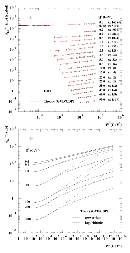
Finally, in fig.9a, we show the GVD/CDP prediction in comparison with the experimental data in the conventional representation of $\sigma_{\gamma^{*}p}(W^{2},Q^{2})$ against $W^{2}$ for fixed $Q^{2}$. A subset of all data used in the fits is presented for illustration.

The explicit analytical form of the theoretical expression for the cross section, $\sigma_{\gamma^{*}p}(W^{2},Q^{2})$, allows us to investigate its behaviour at energies far beyond the ones being explored at HERA. According to (3.6), with (2.33) and (2.35), at any sufficiently large $Q^{2}\raise 1.29167pt\hbox{$>$\kern-7.5pt\raise-4.73611pt\hbox{$\sim$}}\Lambda^{2}(W^{2})$ (i.e. large $\eta$), the cross section increases strongly with energy, as $\Lambda^{2}(W^{2})$, while finally, for sufficiently large energy (i.e. small $\eta$), the hadronlike dependence on energy of photoproduction, will be reached. Explicitly this is demonstrated in fig.9b. While the power-law ansatz and the logarithmic one for $\Lambda^{2}(W^{2})$ coincide at present energies, they differ strongly in how asymptotics will be reached. Unfortunately, the approach to the asymptotic behaviour is slow and can hardly be verified experimentally in the foreseeable future, except, possibly, by the energy dependence of precision data at small values of $Q^{2}\raise 1.29167pt\hbox{$<$\kern-7.5pt\raise-4.73611pt\hbox{$\sim$}}1\mbox{GeV}^{2}$.

Intuitively, a representation of the experimental data on DIS in the low-$x$ diffraction regime in terms of the virtual-photon-proton cross section seems most appropriate and, in particular, reveals the scaling in $\eta$. Nevertheless, for completeness, in fig.10, we show the data for the structure function $F_{2}(x,Q^{2})$ together with the theoretical results of the GVD/CDP.

3.4 A reference to related work

The closest in spirit to the present investigation is the work by Forshaw, Kerley and Shaw [12] and by Golec-Biernat and Wüsthoff [13]. While we agree with the general picture of low-x DIS drawn by these authors, there are numerous essential differences though. In our treatment, the dependence of the colour-dipole cross section on the configuration variable $z$ is taken into account in contrast to refs.[12] and [13]. Our dipole cross section does not depend on $Q^{2}$, in agreement with the mass-dispersion relations (2.15) to (2.18), but in distinction from the $Q^{2}$ (or rather $x$) dependence in ref.[13]. Decent high-energy behaviour at any $Q^{2}$ (“saturation”) follows from the underlying assumptions of colour transparency (the generic two-gluon-exchange structure) and hadronic unitarity in distinction from the two-pomeron ansatz in ref.[12] and in ref.[27] that needs modification at energies beyond the ones explored at HERA.

4 Conclusion

In conclusion, a unique picture, the GVD/CDP, emerges for DIS in the low-x diffraction region. In terms of the (virtual) Compton-forward-scattering amplitude, the photon virtually dissociates into $(q\bar{q})$ vector states that propagate and undergo diffraction scattering from the proton as conjectured in GVD a long time ago. Our knowledge on the photon-$(q\bar{q})$ transition from $e^{+}e^{-}$ annihilation together with the gluon-exchange dynamics from QCD allows for a much more detailed theoretical description of $\sigma_{\gamma^{*}p}(W^{2},Q^{2})$ than available at the time when the GVD approach was formulated. In terms of the GVD/CDP, experiments on DIS at low x measure the energy dependence of the $(q\bar{q})$/colour-dipole-proton cross section, $\sigma_{(q\bar{q})p}(r^{2}_{\bot},z,W^{2})$. A strong energy dependence of this cross section for small interquark separation (not entirely unexpected within the GVD/CDP) is extracted from the data at large $Q^{2}$. The combination of colour transparency (generic two-gluon-exchange structure) with hadronic unitarity then implies that for any interquark separation the strong increase of the colour-dipole cross section with energy, at sufficiently high energy, will settle down to the smooth increase of purely hadronic interactions. The experimental data establish scaling in $\eta$ of $\sigma_{\gamma^{*}p}$. As a consequence, at any fixed value of $Q^{2}$ (at low $x$), $\sigma_{\gamma^{*}p}$ will eventually, at sufficiently high energy, reach the hadronlike behaviour of photoproduction.

Appendix

Appendix A Appendix A

In this Appendix we describe the steps leading from expression (2.1) to (2.15)–(2.18). The Fourier transform of the photon wavefunction as given, for example, in Ref. [8], is in the limit of massless quarks

$${\cal M}_{L}^{(\lambda,\lambda^{\prime})}({\vec{k}}_{\perp},z;Q^{2}) = -\frac{e_{q}z(1\!-\!z)}{(z(1\!-\!z)Q^{2}\!+\!k_{\perp}^{2})}\sqrt{Q^{2}}2\delta_{\lambda,-\lambda^{\prime}}\ ,$$ (A.1)

$${\cal M}_{T,\pm 1}^{(\lambda,\lambda^{\prime})}({\vec{k}}_{\perp},z;Q^{2}) = -\frac{e_{q}}{(z(1\!-\!z)Q^{2}\!+\!k_{\perp}^{2})\sqrt{2}}k_{\perp}{\rm e}^{\pm{\rm i}\varphi}(2z\!-\!1\pm\lambda)\delta_{\lambda,-\lambda^{\prime}}\ ,$$ (A.2)

where $e_{q}$ is the electric charge of quark $q$, $\varphi$ is the azimuthal angle of ${\vec{k}}_{\perp}$ in the plane perpendicular to the proton–photon axis of motion, $\lambda$ and $\lambda^{\prime}$ denote twice the helicities of the quarks $q$ and ${\bar{q}}$, and the signs $\pm$ correspond to the two transverse helicity state polarizations $\epsilon^{\mu}(\pm)=(0,1/\sqrt{2},\pm{\rm i}/\sqrt{2},0)$ of the massive photon in its rest frame. To obtain the total cross section in (2.1), the sum over the helicities $\lambda$ and $\lambda^{\prime}$ is taken, and in the case of the transversely (T) polarized photon $\gamma^{\ast}$ the average over the polarizations $P=\pm 1$

$$\langle|{\cal M}_{L}({\vec{k}}_{\perp},z;Q^{2})|^{2}\rangle \equiv \sum_{\lambda,{\lambda}^{\prime}=\pm 1}|{\cal M}_{L}^{(\lambda,{\lambda}^{\prime})}({\vec{k}}_{\perp},z;Q^{2})|^{2}=\frac{e_{q}^{2}8Q^{2}z^{2}(1\!-\!z)^{2}}{\left[z(1\!-\!z)Q^{2}+{\vec{k}}^{2}_{\perp}\right]^{2}}\ ;$$ (A.3)

$$\langle{\cal M}_{L}({\vec{k}}_{\perp}\!+\!{\vec{l}}_{\perp},z;Q^{2})^{\ast}{\cal M}_{L}({\vec{k}}_{\perp},z;Q^{2})\rangle=\frac{e_{q}^{2}8Q^{2}z^{2}(1\!-\!z)^{2}}{\left[z(1\!-\!z)Q^{2}+{\vec{k}}^{2}_{\perp}\right]\left[z(1\!-\!z)Q^{2}+({\vec{k}}_{\perp}\!+\!{\vec{l}}_{\perp})^{2}\right]}\ ,$$ (A.4)

$$\langle|{\cal M}_{T}({\vec{k}}_{\perp},z;Q^{2})|^{2}\rangle\equiv\frac{1}{2}\!\sum_{P=\pm 1}\sum_{\lambda,{\lambda}^{\prime}=\pm 1}|{\cal M}_{T,P}^{(\lambda,{\lambda}^{\prime})}({\vec{k}}_{\perp},z;Q^{2})|^{2}=2e_{q}^{2}\frac{\left[{\vec{k}}^{2}_{\perp}\left(z^{2}\!+\!(1\!-\!z)^{2}\right)\right]}{\left[z(1\!-\!z)Q^{2}+{\vec{k}}^{2}_{\perp}\right]^{2}}\ ,$$ (A.5)

$$\langle{\cal M}_{T}({\vec{k}}_{\perp}\!+\!{\vec{l}}_{\perp},z;Q^{2})^{\ast}{\cal M}_{T}({\vec{k}}_{\perp},z;Q^{2})\rangle=2e_{q}^{2}\frac{\left[{\vec{k}}_{\perp}\!\cdot\!({\vec{k}}_{\perp}\!+\!{\vec{l}}_{\perp})\left(z^{2}\!+\!(1\!-\!z)^{2}\right)\right]}{\left[z(1\!-\!z)Q^{2}\!+\!{\vec{k}}^{2}_{\perp}\right]\left[z(1\!-\!z)Q^{2}\!+\!({\vec{k}}_{\perp}\!+\!{\vec{l}}_{\perp})^{2}\right]}\ .$$ (A.6)

In (2.1), the integration over ${\vec{k}}^{\prime}_{\perp}$ can be done trivially, resulting in

$$\sigma_{\gamma^{*}_{T,L}p}(W^{2},Q^{2}) = {N_{\rm c}\over{16\pi^{3}}}\int dz\int d^{2}l_{\perp}\tilde{\sigma}_{(q\bar{q})p}(\vec{l}^{~{}2}_{\perp},z,W^{2})$$ (A.7)

$$\times {\Bigg{\{}}\int_{|\vec{k}_{\perp}|\geq k_{\perp 0}}d^{2}k_{\perp}\langle|{\cal M}_{T,L}(\vec{k}_{\perp},z;Q^{2})|^{2}\rangle$$

$$- \int_{|\vec{k}_{\perp}|\geq k_{\perp 0},|{\vec{k}}_{\perp}\!+\!{\vec{l}}_{\perp}|\geq k_{\perp 0}}d^{2}k_{\perp}\langle{\cal M}_{T,L}({\vec{k}}_{\perp}\!+\!{\vec{l}}_{\perp},z;Q^{2})^{\ast}{\cal M}_{T,L}({\vec{k}}_{\perp},z;Q^{2})\rangle{\Bigg{\}}}\ .$$

The multiple integrations in the above expression can be rewritten in the following way. First we rename in all the previous expressions the transfer momentum ${\vec{l}}_{\perp}$ to ${\vec{l}}^{\prime}_{\perp}$. Then we rewrite in the above integrals the Fourier transform ${\tilde{\sigma}}_{(q{\bar{q}})p}(l^{\prime 2}_{\perp},z,W^{2})$ of the colour–dipole cross section as

$${\tilde{\sigma}}_{(q{\bar{q}})p}(l^{\prime 2}_{\perp},z)=\int_{0}^{\infty}dl^{2}_{\perp}{\tilde{\sigma}}_{(q{\bar{q}})p}(l^{2}_{\perp},z)\delta(l^{2}_{\perp}\!-\!l^{\prime 2}_{\perp})\ .$$ (A.8)

The integration over $d^{2}l^{\prime}_{\perp}$ is then to be carried out first. We denote the angle between ${\vec{k}}_{\perp}$ and ${\vec{k}}_{\perp}\!+\!{\vec{l}}^{\prime}_{\perp}$ as $\phi$. We replace $d^{2}l^{\prime}_{\perp}$ by $d^{2}k^{\prime}_{\perp}$ where we identify ${\vec{k}}^{\prime}_{\perp}\equiv{\vec{l}}^{\prime}_{\perp}\!+\!{\vec{k}}_{\perp}$

$$\int_{0}^{1}dz\int d^{2}l^{\prime}_{\perp}{\tilde{\sigma}}_{(q{\bar{q}})p}(l^{\prime 2}_{\perp},z)\int d^{2}k_{\perp}f(k_{\perp},|{\vec{k}}_{\perp}\!+\!{\vec{l}}^{\prime}_{\perp}|,\phi,z)$$ (A.9)

$$= \int_{0}^{1}dz\int dl^{2}_{\perp}{\tilde{\sigma}}_{(q{\bar{q}})p}(l^{2}_{\perp},z)\int d^{2}k_{\perp}\int d^{2}k^{\prime}_{\perp}\delta\left(l^{2}_{\perp}\!-\!({\vec{k}}^{\prime}_{\perp}\!-\!{\vec{k}}_{\perp})^{2}\right)f(k_{\perp},k^{\prime}_{\perp},\phi,z)\ .$$

We now replace $d^{2}k^{\prime}_{\perp}\!\equiv\!(1/2)dk^{\prime 2}_{\perp}d\varphi_{k^{\prime}}$ by $(1/2)dk^{\prime 2}_{\perp}d\phi$, because $\phi=\varphi_{k^{\prime}}\!-\!\varphi_{k}$. The subsequent integration over $d\varphi_{k}$ gives $2\pi$. The above expression reduces to

$$\frac{\pi}{2}\int_{0}^{1}dz\int dl^{2}_{\perp}{\tilde{\sigma}}_{(q{\bar{q}})p}(l^{2}_{\perp},z)\int dk^{2}_{\perp}\int dk^{\prime 2}_{\perp}\int_{0}^{2\pi}d\phi\;\delta(2k_{\perp}k^{\prime}_{\perp}\cos\phi\!-\!k^{2}_{\perp}\!-\!k^{\prime 2}_{\perp}\!+\!l^{2}_{\perp})f(k_{\perp},k^{\prime}_{\perp},\phi,z)\ .$$ (A.10)

The integration over $d\phi$ can now be easily performed, it fixes the value of $\cos\phi$ to a fixed value $\cos\Phi$, and gives

$$\pi\int_{0}^{1}dz\int dl^{2}_{\perp}{\tilde{\sigma}}_{(q{\bar{q}})p}(l^{2}_{\perp},z)\int dk^{2}_{\perp}\int_{(k_{\perp}\!-\!l_{\perp})^{2}}^{(k_{\perp}\!+\!l_{\perp})^{2}}dk^{\prime 2}_{\perp}{\tilde{\omega}}(k_{\perp},k^{\prime}_{\perp},l_{\perp})f(k_{\perp},k^{\prime}_{\perp},\Phi,z)\ ,$$ (A.11)

where

$${\tilde{\omega}}(k_{\perp},k^{\prime}_{\perp},l_{\perp})=\frac{1}{2k_{\perp}k^{\prime}_{\perp}}\frac{1}{\sqrt{1-\cos^{2}\Phi}}\ ,\quad\cos\Phi=\left(\frac{k^{2}_{\perp}\!+\!k^{\prime 2}_{\perp}\!-\!l^{2}_{\perp}}{2k_{\perp}k^{\prime}_{\perp}}\right)\ .$$ (A.12)

The integration limits for $k^{\prime 2}_{\perp}$ in (A.11) are determined by the triangle condition $\cos^{2}\Phi\leq 1$. The fixed angle $\phi=\Phi$ is the angle between the vectors ${\vec{k}}_{\perp}$ and ${\vec{k}}^{\prime}_{\perp}$ and, at the same time, the angle between the vectors ${\vec{k}}_{\perp}$ and ${\vec{k}}_{\perp}\!+\!{\vec{l}}_{\perp}$.

When we trade the variables $k^{2}_{\perp}$ and $k^{\prime 2}_{\perp}$ for $M^{2}\!=\!k^{2}_{\perp}/(z(1\!-\!z))$ (2.6) and $M^{\prime 2}\!=\!k^{\prime 2}/(z(1\!-\!z))$ (2.7), respectively, taking into account the expressions (A.3)–(A.6) in (A.7) and the transformed multiple integration form (A.11), we obtain for the transverse case

$$\sigma_{\gamma^{*}_{T,p}(W^{2},Q^{2})} = {N_{\rm c}\over{16\pi^{3}}}\;2e_{q}^{2}\;\pi\int_{0}^{1}dz\left[z^{2}\!+\!(1\!-\!z)^{2}\right]\int dl^{2}_{\perp}{\tilde{\sigma}}_{(q{\bar{q}})p}(l^{2}_{\perp},z,W^{2})$$ (A.13)

$$\times{\Bigg{\{}}\int_{m_{0}^{2}}^{\infty}dM^{2}\int_{(M\!-\!L_{\perp}(z))^{2}}^{(M\!+\!L_{\perp}(z))^{2}}dM^{\prime 2}\frac{M^{2}}{(Q^{2}\!+\!M^{2})^{2}}\omega(M^{2},M^{\prime 2},L^{2}_{\perp}(z))$$

$$-\int_{m_{0}^{2}}^{\infty}dM^{2}\int_{{\rm max}[m_{0}^{2},(M\!-\!L_{\perp}(z))^{2}]}^{(M\!+\!L_{\perp}(z))^{2}}dM^{\prime 2}\frac{(M^{2}\!+\!M^{\prime 2}\!-\!L^{2}_{\perp}(z))}{2(Q^{2}\!+\!M^{2})(Q^{2}\!+\!M^{\prime 2})}{\Bigg{\}}}\ ,$$

where $L_{\perp}(z)\!\equiv\!l_{\perp}/\sqrt{z(1\!-\!z)}$, the lower cutoff is $m_{0}^{2}\!\equiv\!k^{2}_{\perp 0}/(z(1\!-\!z))$, and $\omega\!=\!z(1\!-\!z){\tilde{\omega}}$

$$\omega(M^{2},M^{\prime 2},L^{2}_{\perp}(z))=\frac{1}{2MM^{\prime}}\frac{1}{\sqrt{1-\cos^{2}\Phi}}\ ,\quad\cos\Phi=\frac{(M^{2}\!+\!M^{\prime 2}\!-\!L^{2}_{\perp}(z))}{2MM^{\prime}}\ .$$ (A.14)

Using the ansatz (2.8) for ${\tilde{\sigma}}_{(q{\bar{q}})p}(l^{2}_{\perp},z,W^{2})$ allows for trivial integration over $l^{2}_{\perp}$, resulting in the additional factor $\sigma^{({\infty})}/\pi$ and the replacement $L_{\perp}(z)\mapsto\Lambda(W^{2})$. Further, if we assume that $m_{0}^{2}$ is $z$–independent, then the integration over $z$ can be done, giving a factor $2/3$. This then gives exactly the result (2.13)–(2.15) and (2.17). The square of the electric charge $e^{2}_{q}$ of the quark $q$ is replaced in general by the sum of the active quark flavours $\sum e_{i}^{2}\!\equiv\!e_{0}^{2}\sum Q_{i}^{2}$ (2.14), and the number of quark colours is $N_{\rm c}=3$.

Formulae (2.16) and (2.18) for the longitudinal polarization can be derived in a completely analogous way.

Appendix B Appendix B

We restrict ourselves to giving the explicit expression for $I^{(1)}_{T}\left(\eta,{{m^{2}_{0}}\over{\Lambda^{2}(W^{2})}}\right)$ and $I^{(1)}_{L}\left(\eta,{{m^{2}_{0}}\over{\Lambda^{2}(W^{2})}}\right)$. Evaluation of the integrals in (2.15) and (2.16) yields

$$I^{(1)}_{T}\left(\eta,\mu\equiv{{m^{2}_{0}}\over{\Lambda^{2}(W^{2})}}\right)$$

$$=\frac{1}{2} \ln\frac{\eta-1+\sqrt{(1+\eta)^{2}-4\mu}}{2\eta}$$ (B.1)

$$+\frac{1+2(\eta-\mu)}{2\sqrt{1+4(\eta-\mu)}}\times \ln\frac{\eta\left(1+\sqrt{1+4(\eta-\mu)}\right)}{4\mu-1-3\eta+\sqrt{\Big{(}1+4(\eta-\mu)\Big{)}\Big{(}(1+\eta)^{2}-4\mu\Big{)}}}$$

$$+\frac{\mu}{\eta}-1$$

and

$$I^{(1)}_{L}\left(\eta,\mu\equiv{{m^{2}_{0}}\over{\Lambda^{2}(W^{2})}}\right)$$

$$=\frac{\eta-\mu}{\sqrt{1+4(\eta-\mu)}}\times \ln\frac{4\mu-1-3\eta+\sqrt{\Big{(}1+4(\eta-\mu)\Big{)}\Big{(}(1+\eta)^{2}-4\mu\Big{)}}}{\eta\left(1+\sqrt{1+4(\eta-\mu)}\right)}$$

$$+ \left(1-\frac{\mu}{\eta}\right).$$

One easily checks that $I^{(1)}_{L}\left(\eta,\mu\equiv{{m^{2}_{0}}\over{\Lambda^{2}(W^{2})}}\right)\to 0$ for $\eta\to\mu$.

Summing $I^{(1)}_{L}$ and $I^{(1)}_{T}$ yields (2.2).

Figure 1: The two-gluon exchange. The arrows relate to the transverse-momentum flow.

Figure 2: Comparision of the result for the correction factor $(1+I^{(2)}/I^{(1)})$ obtained by numerical integration with the result from the analytic approximation (2.30).

Figure 3: The experimental data for $\sigma_{\gamma^{*}p}(W^{2},Q^{2})$ for $x\simeq Q^{2}/W^{2}<0.1$ vs. the low-x scaling variable $\eta=(Q^{2}+m^{2}_{0})/\Lambda^{2}(W^{2})$.

Figure 4: The dependence of $\Lambda^{2}$ on $W^{2}$, as determined by a fit of the GVD/CDP predictions for $\sigma_{\gamma^{*}p}$ to the experimental data.

Figure 5: The GVD/CDP scaling curve for $\sigma_{\gamma^{*}p}$ compared with the experimental data a) for $x<0.01$, b) for $x>0.01$.

Figure 6: The cross section for charm production, $\sigma_{\gamma^{*}p}^{charm}$, in addition to the total cross section, $\sigma_{\gamma^{*}p}$, as a function of $\eta$.

Figure 7: The asymptotic value $\sigma^{(\infty)}(W^{2})$ of the colour-dipole-proton cross section. For comparision, also the photoproduction cross section, multiplied by the factor 240 from $\rho^{0},\omega,\phi$ dominance (2.48), is shown.

Figure 8: The quantity ${\rm P}\cdot\sigma_{\gamma^{*}p}(W^{2},Q^{2})\equiv\frac{6\pi(q^{2}+m_{0}^{2})}{\alpha R_{e^{+}e^{-}}\sigma^{(\infty)}}\sigma_{\gamma^{*}p}(W^{2},Q^{2})$ defined in (3.11) is shown as a function of $W^{2}$ at fixed $Q^{2}$ (a) and as a function of $Q^{2}$ at fixed $W^{2}$ (b). The figure demonstrates that the data for $Q^{2}\raise 1.29167pt\hbox{$>$\kern-7.5pt\raise-4.73611pt\hbox{$\sim$}}10{\rm GeV}^{2}$ yield $\Lambda^{2}(W^{2})$, where $\Lambda^{2}(W^{2})$ determines the energy dependence of the colour-dipole cross section at sufficiently small interquark separation $r_{\perp}$.

Figure 9: The GVD/CDP predictions for $\sigma_{\gamma^{*}p}(W^{2},Q^{2})$ vs. $W^{2}$ at fixed $Q^{2}$  a) in the presently accessible energy range compared with experimental data for $x\leq 0.01$,   b) for asymptotic energies.

Figure 10: The GVD/CDP prediction for the structure function $F_{2}(x,Q^{2})$ in comparision with the experimental data.

References

-
[1]
H1 Collaboration, T. Ahmed et al., Nucl. Phys. B429 (1994) 477;
ZEUS Collaboration, M. Derrick et al., Phys. Lett. B315 (1993) 481;
R. Wichmann, on behalf of the ZEUS and H1 collaborations, Nucl. Phys. B(Proc.Suppl.)82 (2000 )268. -
[2]
J.J. Sakurai and D. Schildknecht, Phys. Lett. 40B (1972) 121;
B. Gorczyca and D. Schildknecht, Phys. Lett. 47B (1973) 71. -
[3]
L. Stodolsky, Phys. Rev. Lett. 18 (1967) 135;
H. Joos, Phys. Lett. B24 (1967) 103. - [4] EM Collab., J. Achman et al., Phys. Lett. B202 (1988) 603.
[5]
D. Schildknecht, Nucl. Phys. B66 (1973) 398;
C.L. Bilchak, D. Schildknecht, J.D. Stroughair, Phys. Lett. B214 (1988) 441; Phys. Lett. B233 (1989) 461. - [6] L. Stodolsky, Phys. Lett. B325 (1994) 505.
- [7] D. Schildknecht, B. Surrow and M. Tentyukov, hep-ph/0010030, Phys. Lett. B499 (2001) 116; D. Schildknecht, contribution to Diffraction 2000, Cetraro, Italy, September 2-7, 2000, hep-ph/0010305, to appear in Nucl. Phys. B, Proceedings Supplements.
- [8] G. Cvetič, D. Schildknecht, A. Shoshi, Eur. Phys. J. C 13 (2000) 301; Acta Physica Polonica B30 (1999) 3265; D. Schildknecht, Contribution to DIS 2000 (Liverpool, April 2000), hep-ph/0006153.
- [9] J. Gunion and D. Soper, Phys. Rev. D15, 2617 (1977).
[10]
H. Fraas, B. Read and D. Schildknecht, Nucl. Phys. B86, (1975) 346;
R. Devenish, D. Schildknecht Phys. Rev. D14 (1976) 93. - [11] N.N. Nikolaev and B.G. Zakharov,Z. Phys. C49 (1991) 607.
[12]
J. Forshaw, G. Kerley and G. Shaw, Phys. Rev. D60
(1999) 074012, hep-ph/9903341;
Contribution to DIS2000 (Liverpool, April 2000), hep-ph/0007257. -
[13]
K. Golec-Biernat and M. Wüsthoff, Phys. Rev. D59
(1999) 014017; Phys. Rev. D60 (1999) 114023;
A.M. Stasto, K. Golec-Biernat and J. Kwiecinski, hep-ph 0007192. - [14] J.D. Bjorken, hep-ph/9601363.
[15]
J.J. Sakurai, Currents and Mesons, The University of Chicago Press,
Chicago, 1969;
D. Schildknecht, Springer Tracts in Modern Physics, vol.63 (1972) p. 57;
A. Donnachie and G. Shaw, in: A. Donnachie, G. Shaw (Eds.), Electromagnetic Interactions of Hadrons, vol. 2, Plenum Press, New York 1978, p. 169;
G. Grammar, Jr., Jeremiah D. Sullivan, ibid. p. 195. - [16] D. Schildknecht and F. Steiner, Phys. Lett. 56B (1975) 36
[17]
ZEUS 94: ZEUS Collab., M. Derrick et al., Z. f. Physik C72 (1996) 399.
ZEUS SVTX 95: ZEUS Collab., J. Breitweg et al., Eur. Phys. J. C7 (1999) 609.
ZEUS BPC 95: ZEUS Collab., J. Breitweg et al., Phys. Lett. B407 (1997) 432.
ZEUS BPT 97: ZEUS Collab., J. Breitweg et al., Phys. Lett. B487 (2000) 1-2, 53. -
[18]
H1 SVTX 95: H1 Collab., C. Adloff et al., Nucl. Phys. B497 (1997) 3.
H1 94: H1 Collab., S. Aid et al., Nucl. Phys. B470 (1996) 3.
H1 97: H1 Collab., C. Adloff et al., Eur. Phys. J. C13 (2000) 609. -
[19]
D. Schildknecht,
H. Spiesberger, hep-ph/9707447; D. Schildknecht, Acta Phys. Pol. B28,
2453 (1997);
D. Schildknecht, in Proc. of the XXXIIIrd Recontres de Moriond, ‘98 QCD and High Energy Hadronic Interactions, ed. by J. Trân Thanh Vân (Edition Frontières 1998), p. 461; hep-ph/9806353. - [20] L. Frankfurt, V. Guzey, M. Strikman, Phys. Rev. D58 (1998) 094039; hep-ph/9712339
- [21] M. Böhm, H. Joos and M. Krammer, Acta Phys. Austriaca 38 (1973) 123.
- [22] E665 Collab., Adams et al., Phys. Rev. D54 (1996) 3006.
- [23] NMC Collab., Arneodo et al., Nucl. Phys. B483 (1997) 3.
- [24] BCDMS Collab., Benvenuti et al., Phys. Lett. B223 (1989) 485.
[25]
ZEUS Collab., J. Breitweg et al., Eur. Phys. J. C7
(1999) 609,
B. Surrow, Eur. Phys. J. direct C 2 (1999), 1. -
[26]
H1 Collab., C. Adloff et al., Zeit.Phys. C72 (1996) 503;
ZEUS Collab., J. Breitweg et al., Phys.Lett. B407 (1997) 402. - [27] A. Donnachie and P.V. Landshoff, Phys. Lett. B437 (1998) 408.
- [28] M.F. McDermott, DESY00-126, hep-ph/0008260.