The anomalous process $\gamma\pi\rightarrow\pi\pi$ to two loops

Abstract

The amplitude for the anomalous process $\gamma\pi\rightarrow\pi\pi$ is evaluated to two loops in the chiral expansion by means of a dispersive method. The two new coupling constants that enter at this order are estimated via sum rules derived from a non-perturbative chiral approach. With these coupling constants fixed, the numerical results are given and compared with the available experimental information.

1 Introduction

At low energies, the strong interaction between pions can be described by the effective field theory of QCD called chiral perturbation theory (ChPT) [1, 2, 3, 4]. In this effective field theory the interaction between pions is analyzed in terms of a systematic expansion in powers of the low external momenta and the small pion mass. This chiral expansion is equivalent to an expansion in the number of loops and works very well for processes involving pions [5].

In the normal intrinsic parity sector, the chiral expansion starts at $O(p^{2})$ and is obtained from the leading order chiral Lagrangian. In this sector the one-loop or $O(p^{4})$ corrections were extensively treated in the works by Gasser and Leutwyler [2, 3], and many processes have now been calculated to this order. The further extension to two loops of $O(p^{6})$ has also been undertaken with several two-flavour calculations already published in the normal sector [6, 7, 8, 9, 10].

For the abnormal intrinsic parity sector, the chiral expansion starts at $O(p^{4})$ and is obtained from the Wess-Zumino-Witten effective action [11]. In this sector the one-loop corrections of $O(p^{6})$ have also been analyzed [12], and some anomalous processes have been calculated to this order [13]. However, contrary to the case in the normal sector, no two-loop calculations of $O(p^{8})$ have been published for processes in the anomalous sector.

In this paper the anomalous process $\gamma\pi\rightarrow\pi\pi$ is calculated to two loops using a dispersive method. This process is important for the theory of chiral anomalies and has previously been calculated to both leading [14] and one-loop [15] order in the chiral expansion. However, both of these results are somewhat below the present experimental data [16]. This has motivated new and more precise experiments, which will be performed at different facilities such as CERN [17], FNAL [18], and CEBAF [19].

It is therefore important to evaluate the two-loop corrections and compare the result with the experimental information. This is the purpose of the present paper, which is organized as follows. In Sect. 2, the notation and kinematics of the process $\gamma\pi\rightarrow\pi\pi$ are given, whereas previous ChPT results are reviewed in Sect. 3. The general dispersive formula is derived in Sect. 4, together with the explicit calculation of the two-loop corrections. In Sect. 5, this two-loop result is used in a non-perturbative chiral approach in order to estimate the two new coupling constants from sum rules. The numerical results are given in Sect. 6, including the comparison with experiments, and Sect. 7 consists of a short conclusion.

2 Kinematics

The amplitude for the anomalous process

$$\gamma(q)\pi^{-}(p_{1})\rightarrow\pi^{-}(p_{2})\pi^{0}(p_{0})$$ (1)

is given in terms of the scalar function $F_{3\pi}(s,t,u)$ as

$$A=iF_{3\pi}(s,t,u)\epsilon^{\mu\nu\alpha\beta}\epsilon_{\mu}p_{1\nu}p_{2\alpha}p_{0\beta},$$ (2)

where $s=(p_{1}+q)^{2}$, $t=(p_{1}-p_{2})^{2}$, and $u=(p_{1}-p_{0})^{2}$ are the Mandelstam variables. In the following it is assumed that all particles are real. In this case $s+t+u=3M^{2}_{\pi}$, so that in the center of mass system one has

$$t = \frac{1}{2}\left[3M^{2}_{\pi}-s+(s-M^{2}_{\pi})\sqrt{1-4M^{2}_{\pi}/s}\cos\theta\right],$$

$$u = \frac{1}{2}\left[3M^{2}_{\pi}-s-(s-M^{2}_{\pi})\sqrt{1-4M^{2}_{\pi}/s}\cos\theta\right]$$ (3)

with $\theta$ the center of mass scattering angle. Because of isospin symmetry, the other $\gamma\pi\rightarrow\pi\pi$ reactions are given by the same scalar function $F_{3\pi}(s,t,u)$, which is fully symmetrical in its arguments. The total cross section is obtained from the expression

$$\sigma(s)=\frac{1}{1024\pi}\frac{(s-4M_{\pi}^{2})^{3/2}}{s^{1/2}}(s-M_{\pi}^{2})\int_{0}^{\pi}d\theta\sin^{3}\theta|F_{3\pi}(s,t,u)|^{2},$$ (4)

and the partial wave expansion of the scalar function $F_{3\pi}(s,t,u)$ is of the form

$$F_{3\pi}(s,t,u)=\sum_{odd\;l}f_{l}(s)P_{l}^{\prime}(\cos\theta).$$ (5)

The projection onto the lowest $P$ partial wave is given by

$$f_{1}(s)=\frac{3}{8\pi}\int d\Omega\sin^{2}\theta F_{3\pi}(s,t,u),$$ (6)

and the higher partial waves can be projected out in similar ways. This partial wave expansion contains only odd $l$ since the pions in the final state have the total isospin $I=1$. In the unitarity relation, the complete set of intermediate states are the same as for $\pi\pi$ scattering. Within the elastic approximation containing only the two-pion intermediate state, the unitarity relation is

$${\rm Im}f_{l}(s)=\sigma(s)f_{l}^{\ast}(s)t^{1}_{l}(s)$$ (7)

with $\sigma(s)=\sqrt{(s-4M_{\pi}^{2})/s}$ the phase-space factor and $t^{1}_{l}$ the $\pi\pi$ partial wave with isospin $I=1$ and angular momentum $l$. This unitarity relation implies that the phase of $f_{l}$ will coincide with the $\pi\pi$ phase shift $\delta^{1}_{l}$ in accordance with Watson’s final-state theorem [20]. Inelasticities due to other intermediate states such as the four-pion or the $K\bar{K}$ states remain very small below 1 GeV and are completely negligible at low energies.

3 Chiral expansion

Anomalous processes start at $O(p^{4})$ in the chiral expansion and are obtained from the Wess-Zumino-Witten effective action at tree level. With only the electromagnetic interaction as external fields, these anomalous processes contain exclusively an odd number of pseudoscalars, i.e., they have abnormal or odd intrinsic parity. For the process $\gamma\pi\rightarrow\pi\pi$, the leading order chiral result for the scalar function $F_{3\pi}(s,t,u)$ is given by [11, 14]

$$F_{3\pi}(s,t,u)=F_{3\pi}^{(0)}=\frac{eN_{c}}{12\pi^{2}F_{\pi}^{3}},$$ (8)

where $N_{c}=3$ is the number of colors and $F_{\pi}=92.4$ MeV is the pion decay constant. Another related anomalous process is the decay $\pi^{0}\rightarrow\gamma\gamma$, where the $F_{\pi\gamma\gamma}$ coupling obtained at leading order is of the form [11, 21]

$$F^{(0)}_{\pi\gamma\gamma}=\frac{\alpha N_{c}}{3\pi F_{\pi}}.$$ (9)

These two results are exact in the soft pion and soft photon limit where they are related to each other by the low-energy theorem $F_{3\pi}=F_{\pi\gamma\gamma}/eF_{\pi}^{2}$. For the decay $\pi^{0}\rightarrow\gamma\gamma$, the prediction from Eq. (9) is in excellent agreement with the experimental information, thus providing important evidence for the three-color nature of the strong interaction. However, for the process $\gamma\pi\rightarrow\pi\pi$, the corresponding prediction $F_{3\pi}=9.7$ ${\rm GeV}^{-3}$ is somewhat lower than the experimental measurement $F_{3\pi}=12.9\pm 0.9\pm 0.5$ ${\rm GeV}^{-3}$ [16], which could even be said to favor the value $N_{c}=4$.

It is therefore of importance to calculate the corrections to the soft pion and soft photon limit. Within ChPT these corrections can indeed be calculated in a systematic manner. The first correction is the one-loop contribution of $O(p^{6})$, which has previously been calculated for both processes. In the case of the decay $\pi^{0}\rightarrow\gamma\gamma$, these one-loop corrections turn out to be very small [22], i.e., they do not spoil the excellent agreement with the experimental information. On the other hand, for the process $\gamma\pi\rightarrow\pi\pi$, the one-loop contributions are larger and they will therefore be of importance when comparing with the experimental measurement. The expression for the scalar function $F_{3\pi}(s,t,u)$ to this order in the chiral expansion is [15]

$$F_{3\pi}(s,t,u)=F_{3\pi}^{(0)}\left[1-\frac{64\pi^{2}}{3e}C_{2}^{r}(\mu)(s+t+u)+C_{l}^{\pi}\right],$$ (10)

where the term $C_{l}^{\pi}$ contains the contributions from the loops and is given by

$$C_{l}^{\pi} = \frac{1}{96\pi^{2}F_{\pi}^{2}}\left[-(s+t+u)\log\frac{M_{\pi}^{2}}{\mu^{2}}+\frac{5}{3}(s+t+u)\right]$$ (11)

$$+\frac{1}{24\pi^{2}F_{\pi}^{2}}\left[F(s)+F(t)+F(u)\right]$$

with $F(x)$ expressed in terms of the standard one-loop function $\bar{J}(x)$ as

$$F(x)=4\pi^{2}(x-4M_{\pi}^{2})\bar{J}(x)-\mbox{$\frac{1}{2}$}x.$$ (12)

The expression (10) converges to the chiral anomaly $F_{3\pi}^{(0)}$ in the soft pion and soft photon limit and is given in terms of the renormalized low-energy constant $C_{2}^{r}$ from the $O(p^{6})$ anomalous chiral Lagrangian [12]. This low-energy constant depends on the renormalization scale $\mu$ and is needed to absorb divergences in the one-loop calculation. In principle, $C_{2}^{r}$ should be determined phenomenologically, preferably from other observables, but at present this appears to be rather out of reach. Therefore, this low-energy constant has been estimated using the assumption of vector resonance saturation, which is known to work well for the $O(p^{4})$ non-anomalous low-energy constants [23]. Assuming that the same is the case for the $O(p^{6})$ anomalous low-energy constants, one has [15]

$$C_{2}^{r}(\mu)=-\frac{3e}{128\pi^{2}M_{\rho}^{2}}$$ (13)

with the renormalization scale typical chosen at the resonance scale $\mu=M_{\rho}=770$ MeV. Having fixed the value of this low-energy constant, it is possible to obtain the prediction for the one-loop expression (10). This improves the agreement with the experimental measurement [16]. However, the prediction is still on the lower side of the data [15, 17, 18].

Therefore, it is important with both theoretical and experimental improvements. Indeed, significant improvements on the experimental side are expected from several new experiments [17, 18, 19]. A similar improvement on the theoretical side would involve the calculation of the two-loop corrections. This could be done by a full field theory calculation to two loops. However, these two-loop corrections can also be calculated by a dispersive method, which will be the subject of the next section.

4 Dispersive representation

4.1 Derivation of the dispersive formula

The anomalous process $\gamma\pi\rightarrow\pi\pi$ is in many ways similar to the $\pi^{0}\pi^{0}\rightarrow\pi^{0}\pi^{0}$ scattering process. They are both described in terms of a single scalar function, which is fully symmetrical in the $s$, $t$, and $u$ variables. The $\pi\pi$ scattering process can be described by Roy equations [24] derived from the fundamental principles of analyticity, crossing, and unitarity. When these Roy equations are combined with the chiral expansion, the general structure of the $\pi\pi$ scattering amplitude can be obtained from a dispersive representation to two loops in the chiral expansion [8, 25].

The same is also the case for the process $\gamma\pi\rightarrow\pi\pi$. In order to show this, one starts with a fixed-t dispersion relation for the scalar function $F_{3\pi}(s,t,u)$. Fixed-t dispersion relations with two subtractions are known to exist for $\pi\pi$ scattering due to the Froissart bound. Assuming that the same is also the case for the process $\gamma\pi\rightarrow\pi\pi$, one has the fixed-t dispersion relation

$$F_{3\pi}(s,t)=C(t)+\frac{1}{\pi}\int_{4M_{\pi}^{2}}^{\infty}ds^{\prime}\frac{{\rm Im}F_{3\pi}(s^{\prime},t)}{s^{\prime 2}}\left(\frac{s^{2}}{s^{\prime}-s}+\frac{u^{2}}{s^{\prime}-u}\right),$$ (14)

where $u=3M_{\pi}^{2}-s-t$. The $s\leftrightarrow u$ symmetry of $F_{3\pi}(s,t,u)$ implies that there is no subtraction constant linear in $s$. Therefore, the only subtraction constant is $C(t)$, where the $t$ dependence can be obtained from the $s\leftrightarrow t$ symmetry $F_{3\pi}(0,t)=F_{3\pi}(t,0)$. This implies that $C(t)$ can be written as

$$C(t) = C(0)+\frac{1}{\pi}\int_{4M_{\pi}^{2}}^{\infty}ds^{\prime}\frac{{\rm Im}F_{3\pi}(s^{\prime},0)}{s^{\prime 2}}\left(\frac{t^{2}}{s^{\prime}-t}+\frac{(3M_{\pi}^{2}-t)^{2}}{s^{\prime}-3M_{\pi}^{2}+t}\right)$$ (15)

$$-\frac{1}{\pi}\int_{4M_{\pi}^{2}}^{\infty}ds^{\prime}\frac{{\rm Im}F_{3\pi}(s^{\prime},t)}{s^{\prime 2}}\frac{(3M_{\pi}^{2}-t)^{2}}{s^{\prime}-3M_{\pi}^{2}+t},$$

which can be inserted in Eq. (14). By construction, the resulting dispersion relation exhibits $s\leftrightarrow u$ symmetry for fixed $t$, whereas $s\leftrightarrow t$ symmetry for fixed $u$ is not manifest. In order to impose this latter symmetry one can expand the absorptive part of $F_{3\pi}(s^{\prime},t)$ in partial waves using Eq. (5). Writing this expansion in the form

$${\rm Im}F_{3\pi}(s^{\prime},t)={\rm Im}f_{1}(s^{\prime})+{\rm Im}\Phi(s^{\prime},t),$$ (16)

the higher partial waves with $l\geq 3$ are contained in the function ${\rm Im}\Phi(s^{\prime},t)$, which is given by

$${\rm Im}\Phi(s^{\prime},t)=\sum_{l\geq 3}{\rm Im}f_{l}(s^{\prime})P_{l}^{\prime}(\cos\theta).$$ (17)

With this decomposition of the partial waves, it is possible to rewrite Eq. (14) with $C(t)$ given by Eq. (15) as

$$F_{3\pi}(s,t,u)=\hat{F}_{3\pi}(s,t,u)+\Phi_{3\pi}(s,t,u),$$ (18)

where $\hat{F}_{3\pi}(s,t,u)$ and $\Phi_{3\pi}(s,t,u)$ are given by

$$\hat{F}_{3\pi}(s,t,u) = C(0)+\frac{1}{\pi}\int_{4M_{\pi}^{2}}^{\infty}ds^{\prime}\frac{{\rm Im}f_{1}(s^{\prime})}{s^{\prime 2}}\left(\frac{s^{2}}{s^{\prime}-s}+\frac{t^{2}}{s^{\prime}-t}+\frac{u^{2}}{s^{\prime}-u}\right),$$

$$\Phi_{3\pi}(s,t,u) = \frac{1}{\pi}\int_{4M_{\pi}^{2}}^{\infty}ds^{\prime}\frac{{\rm Im}\Phi(s^{\prime},t)}{s^{\prime 2}}\left(\frac{s^{2}}{s^{\prime}-s}+\frac{u^{2}}{s^{\prime}-u}-\frac{(3M_{\pi}^{2}-t)^{2}}{s^{\prime}-3M_{\pi}^{2}+t}\right)$$ (19)

$$+\frac{1}{\pi}\int_{4M_{\pi}^{2}}^{\infty}ds^{\prime}\frac{{\rm Im}\Phi(s^{\prime},0)}{s^{\prime 2}}\left(\frac{t^{2}}{s^{\prime}-t}+\frac{(3M_{\pi}^{2}-t)^{2}}{s^{\prime}-3M_{\pi}^{2}+t}\right).$$

This is the Roy equation for the anomalous process $\gamma\pi\rightarrow\pi\pi$. One observes that $\hat{F}_{3\pi}(s,t,u)$ is now fully symmetrical in $s$, $t$, and $u$, whereas this symmetry is not manifest in $\Phi_{3\pi}(s,t,u)$. However, at low energies, the absorptive part of the higher partial waves with $l\geq 3$ is negligible. This implies that in practice $\Phi_{3\pi}(s,t,u)$ can be treated in a simple way as a small, real correction at low energies. This fact makes the corresponding Roy equations for $\pi\pi$ scattering very useful.

In ChPT the absorptive part of the higher partial waves is indeed suppressed. Within this methodology, these higher partial waves only start at $O(p^{6})$ in the chiral expansion. Since the corresponding $\pi\pi$ partial waves start at $O(p^{4})$, perturbative unitarity implies that the absorptive part of the higher partial waves with $l\geq 3$ is of $O(p^{10})$ or higher in the chiral expansion. Thus, up to this order, the term $\Phi_{3\pi}(s,t,u)$ in Eq. (18) vanishes, and the full amplitude is given entirely by the function $\hat{F}_{3\pi}(s,t,u)$. In order for the full amplitude to formally satisfy the chiral anomaly in the soft pion and soft photon limit, one may write the subtraction constant as $C(0)=F_{3\pi}^{(0)}[1+\bar{C}(s+t+u)]$, where $s+t+u=3M_{\pi}^{2}$. Thus, assuming for the moment that two subtractions are indeed sufficient, the full amplitude to $O(p^{8})$ in the chiral expansion may be written as

$$F_{3\pi}(s,t,u) = F_{3\pi}^{(0)}\left[1+\bar{C}(s+t+u)\right]$$ (20)

$$+\frac{1}{\pi}\int_{4M_{\pi}^{2}}^{\infty}ds^{\prime}\frac{{\rm Im}f_{1}(s^{\prime})}{s^{\prime 2}}\left(\frac{s^{2}}{s^{\prime}-s}+\frac{t^{2}}{s^{\prime}-t}+\frac{u^{2}}{s^{\prime}-u}\right).$$

In this dispersive representation, the absorptive part of the lowest partial wave can be determined from unitarity. In the general unitarity relation, the $2n$-pion invariant phase space is of $O(p^{4n-4})$, the amplitude for multi-pion scattering is dominantly of $O(p^{2})$, and the amplitude for multi-pion photo-production is at least of $O(p^{4})$. Consequently, intermediate states containing more than two pions are suppressed at least up to $O(p^{10})$ in the chiral expansion. Therefore, within SU(2) ChPT, the absorptive part of the lowest partial wave is given by elastic unitarity to $O(p^{8})$ as

$${\rm Im}f_{1}^{(0)}(s) = 0,$$

$${\rm Im}f_{1}^{(1)}(s) = \sigma(s)f_{1}^{(0)}(s)t^{1(0)}_{1}(s),$$

$${\rm Im}f_{1}^{(2)}(s) = \sigma(s)\left[f_{1}^{(0)}(s){\rm Re}t^{1(1)}_{1}(s)+{\rm Re}f_{1}^{(1)}(s)t^{1(0)}_{1}(s)\right],$$ (21)

where $f_{1}^{(n)}$ is the $P$ partial wave of $O(p^{2n+4})$ and $t_{1}^{1(n)}$ the corresponding $\pi\pi$ partial wave of $O(p^{2n+2})$ [2]. In SU(3) ChPT, one must also include the inelasticity from the $K\bar{K}$ intermediate state. However, since this inelasticity is completely negligible at low energies, only SU(2) ChPT will be considered in the following.

4.2 The amplitude to two loops

From the dispersive representation (20), one obtains straightforwardly the one-loop ChPT formula (10) by setting ${\rm Im}f_{1}={\rm Im}f_{1}^{(1)}$. In this case the subtraction constant $\bar{C}$ can be expressed in terms of the low-energy constant $C_{2}^{r}$ and chiral logarithms. However, in order to calculate the amplitude to two loops, it is necessary to use one subtraction more in the dispersive representation. This is due to the fact that the absorptive part of $f_{1}^{(2)}$ behaves as $s^{2}$ modulo log factors. Thus, the amplitude to two loops can be obtained from the following dispersion relation:

$$F_{3\pi}(s,t,u) = F_{3\pi}^{(0)}\left[1+\bar{C}(s+t+u)+\bar{D}(s^{2}+t^{2}+u^{2})\right]$$ (22)

$$+\frac{1}{\pi}\int_{4M_{\pi}^{2}}^{\infty}ds^{\prime}\frac{{\rm Im}f_{1}(s^{\prime})}{s^{\prime 3}}\left(\frac{s^{3}}{s^{\prime}-s}+\frac{t^{3}}{s^{\prime}-t}+\frac{u^{3}}{s^{\prime}-u}\right),$$

where $\bar{C}$ and $\bar{D}$ are the two subtraction constants and ${\rm Im}f_{1}$ is given by ${\rm Im}f_{1}={\rm Im}f_{1}^{(1)}+{\rm Im}f_{1}^{(2)}$ with ${\rm Im}f_{1}^{(1)}$ and ${\rm Im}f_{1}^{(2)}$ determined from Eq. (4.1). This dispersion relation can be evaluated with the same methodology as has been applied in the calculation of the $\pi\pi$ scattering amplitude [8] and the pion form factors [6] to two loops. With the use of this methodology, the result can be written as

$$F_{3\pi}(s,t,u) = F_{3\pi}^{(0)}\left[1+\bar{C}(s+t+u)+\bar{D}(s^{2}+t^{2}+u^{2})\right.$$ (23)

$$\left.+U^{A}(s)+U^{A}(t)+U^{A}(u)+U^{\Delta}(s)+U^{\Delta}(t)+U^{\Delta}(u)\right],$$

where the $U^{A}$ term can be expressed in the compact analytic form:

$$U^{A}(x) = \frac{M_{\pi}^{2}}{16\pi^{2}F_{\pi}^{2}}\left\{\frac{x}{9M_{\pi}^{2}}\left[1+24\pi^{2}\sigma^{2}(x)\bar{J}(x)\right]-\frac{x^{2}}{60M_{\pi}^{4}}\right\}+\left(\frac{M_{\pi}^{2}}{16\pi^{2}F_{\pi}^{2}}\right)^{2}$$ (24)

$$\times\left\{\left[\bar{l}_{2}-\bar{l}_{1}+\frac{6M_{\pi}^{2}\bar{l}_{4}}{x}+\frac{9M_{\pi}^{2}\bar{c}_{1}}{x}\right]\frac{x^{2}}{27M_{\pi}^{4}}\left[1+24\pi^{2}\sigma^{2}(x)\bar{J}(x)\right]\right.$$

$$-\frac{x^{2}}{30M_{\pi}^{4}}\bar{l}_{4}-\frac{x^{2}}{20M_{\pi}^{4}}\bar{c}_{1}+\frac{3191}{6480}\frac{x^{2}}{M_{\pi}^{4}}+\frac{223}{216}\frac{x}{M_{\pi}^{2}}-\frac{16}{9}$$

$$-\frac{\pi^{2}x}{540M_{\pi}^{2}}\left(37\frac{x}{M_{\pi}^{2}}+15\right)+\frac{4\pi^{2}}{27}\left(7\frac{x^{2}}{M_{\pi}^{4}}-151\frac{x}{M_{\pi}^{2}}+99\right)\bar{J}(x)$$

$$+\frac{2\pi^{2}M_{\pi}^{2}}{9x}\left(\frac{x^{3}}{M_{\pi}^{6}}-30\frac{x^{2}}{M_{\pi}^{4}}+78\frac{x}{M_{\pi}^{2}}-128\right)\bar{K}_{1}(x)$$

$$\left.+8\pi^{2}\left(\frac{x^{2}}{M_{\pi}^{4}}-\frac{13}{3}\frac{x}{M_{\pi}^{2}}-2\right)\bar{K}_{4}(x)\right\}.$$

The explicit expressions for the functions $\bar{K}_{1}(x)$ and $\bar{K}_{4}(x)$ are given in Ref. [8], where these functions were introduced in the evaluation of the $\pi\pi$ scattering amplitude to two loops. They are analytic functions with cuts starting at the $\pi\pi$ threshold and can be expressed in terms of the standard one-loop function $\bar{J}(x)$. As for the other term $U^{\Delta}$, this part does not have a compact analytic representation in terms of elementary functions. However, it can be obtained numerically from the dispersive representation:

$$U^{\Delta}(x)=\frac{x^{3}}{\pi}\int_{4M_{\pi}^{2}}^{\infty}ds^{\prime}\frac{\sigma(s^{\prime}){\rm Re}f_{1}^{\Delta}(s^{\prime})t_{1}^{1(0)}(s^{\prime})}{s^{\prime 3}(s^{\prime}-x)}.$$ (25)

In this dispersive formula $t_{1}^{1(0)}$ is the lowest order $\pi\pi$ $P$ partial wave and $f_{1}^{\Delta}$ is given by

$$f_{1}^{\Delta}(s)=\frac{3}{8\pi}\int d\Omega\sin^{2}\theta\frac{1}{96\pi^{2}F_{\pi}^{2}}\left\{\frac{5}{3}(t+u)+4[F(t)+F(u)]\right\}$$ (26)

with $t$ and $u$ determined from Eq. (2) and $F(x)$ given by Eq. (12). The size of the corrections from $U^{\Delta}$ are very small at low energies and they can therefore in practice be neglected at these energies.

In the dispersive representation, Eq. (23), the full amplitude to two loops is determined up to the subtraction constants $\bar{C}$ and $\bar{D}$. These subtraction constants may be parameterized in terms of the coupling constants $\bar{c}_{1}$, $\bar{c}_{2}$, and $\bar{d}_{2}$ as

$$\bar{C} = \frac{1}{16\pi^{2}F_{\pi}^{2}}\left[(\bar{c}_{1}-\mbox{$\frac{1}{6}$})+\frac{M_{\pi}^{2}}{16\pi^{2}F_{\pi}^{2}}\bar{c}_{2}\right],$$

$$\bar{D} = \frac{1}{16\pi^{2}F_{\pi}^{2}}\left[\frac{1}{60M_{\pi}^{2}}+\frac{1}{16\pi^{2}F_{\pi}^{2}}\bar{d}_{2}\right],$$ (27)

where the coupling constant $\bar{c}_{1}$ can be expressed in terms of the $O(p^{6})$ anomalous low-energy constant $C_{2}^{r}$ and chiral logarithms:

$$\bar{c}_{1}=16\pi^{2}F_{\pi}^{2}\left[-\frac{64\pi^{2}}{3e}C_{2}^{r}(\mu)-\frac{1}{96\pi^{2}F_{\pi}^{2}}\log\frac{M_{\pi}^{2}}{\mu^{2}}\right].$$ (28)

The coupling constants $\bar{c}_{2}$ and $\bar{d}_{2}$ enter at two-loop order in the chiral expansion and contain contributions both from two-loop diagrams and from the unknown renormalized low-energy constants, which parameterize the $O(p^{8})$ anomalous chiral Lagrangian.

5 Non-perturbative chiral approach

5.1 The lowest partial wave

From the two-loop expression for the amplitude, Eq. (23), one may project out the lowest $P$ partial wave with the use of Eq. (6). This gives the expansion

$$f_{1}(s)=f_{1}^{(0)}(s)+f_{1}^{(1)}(s)+f_{1}^{(2)}(s),$$ (29)

which will satisfy the perturbative unitarity relations (4.1). These relations work very well at low energies, whereas the deviation from exact unitarity, Eq. (7), becomes more pronounced as the energy is increased. At these energies, still higher order unitarity corrections will start to be of importance in the chiral expansion. This is particularly the case in the $\rho$(770) resonance region, where unitarity corrections are essential.

In the presence of the $\rho$(770) resonance, unitarity will therefore be of the utmost importance. There are different ways to combine exact unitarity and the chiral expansion in order to try to account for this resonance. One such method, which has been successfully applied to many different processes, is the so-called non-perturbative inverse amplitude method (IAM) [26, 27, 28, 29]. Since this is a rather general method, it can also be straightforwardly applied to the present case. The starting point for the IAM is to write down a dispersion relation for the inverse of the partial wave $f_{1}$. In this dispersion relation, exact unitarity and the chiral expansion are used to compute the important right cut, whereas the left cut and the subtraction constants are approximated by ChPT. If one writes down a similar dispersion relation for the chiral expansion using perturbative unitarity on the right cut, it is possible to express the result of the IAM in a simple way in terms of the chiral partial waves. With the two-loop ChPT expansion (29), the result of the IAM can be written as

$$f_{1}(s)=\frac{{f_{1}^{(0)}}^{2}(s)}{f_{1}^{(0)}(s)-f_{1}^{(1)}(s)+{f_{1}^{(1)}}^{2}(s)/f_{1}^{(0)}(s)-f_{1}^{(2)}(s)}.$$ (30)

This is formally equivalent to the [0,2] Padé approximant applied to ChPT and will therefore coincide with the chiral expansion up to two loops. However, since exact unitarity was used in the derivation of the IAM, it is expected that this result will improve ChPT at higher energies. The IAM applied to two-loop ChPT has been extensively discussed in Ref. [28], where the detailed derivation of the general result can also be found.

The result of the IAM, Eq. (30), depends on the pion mass and pion decay constant, which will be set equal to $M_{\pi}=139.6$ MeV and $F_{\pi}=92.4$ MeV, respectively. Furthermore, the IAM is also given in terms of the low-energy constants $\bar{l}_{2}-\bar{l}_{1}$ and $\bar{l}_{4}$. These low-energy constants appear in the ChPT $\pi\pi$ $P$ partial wave to one loop order and can been determined phenomenologically from other sources. However, since the IAM contains higher order unitarity corrections, the phenomenological values of these low-energy constants in the IAM do not necessarily coincide precisely with the values obtained in ChPT. For the combination $\bar{l}_{2}-\bar{l}_{1}$, this has been determined by applying the IAM to one-loop ChPT in the case of $\pi\pi$ scattering with the result $\bar{l}_{2}-\bar{l}_{1}=5.8$ [28]. The other low-energy constant $\bar{l}_{4}$ has been determined in ChPT from the pion scalar form factor with the central value $\bar{l}_{4}=4.4$ [7]. Since the IAM (30) does not depend much on the precise value of this low-energy constant, the same value can also be applied in the IAM. Finally, this result also depends on the one-loop coupling constant $\bar{c}_{1}$. This coupling constant is related to the low-energy constant $C_{2}^{r}$, which has been estimated from the assumption of vector resonance saturation, Eq. (13) [15]. With the value of $C_{2}^{r}$ chosen at the renormalization scale $\mu=M_{\rho}$, one finds $\bar{c}_{1}=1.71$. Therefore, in the IAM (30), the values

$$\bar{l}_{2}-\bar{l}_{1}=5.8\;\;\;\;,\;\;\;\;\bar{l}_{4}=4.4\;\;\;\;,\;\;\;\;\bar{c}_{1}=1.71$$ (31)

will be used throughout. Having fixed these constants, it is possible to determine the remaining two-loop coupling constants $\bar{c}_{2}$ and $\bar{d}_{2}$ in the IAM from the mass and width of the $\rho$(770) resonance. The mass of this resonance can be defined as the energy where the phase passed $90^{\circ}$ and the width can be determined from the slope of the phase at the resonance. With $M_{\rho}=770.0$ MeV and $\Gamma_{\rho}=150.7$ MeV [30], this gives the values

$$\bar{c}_{2}=-27\;\;\;\;,\;\;\;\;\bar{d}_{2}=3.477,$$ (32)

where the IAM depends rather strongly on $\bar{d}_{2}$ and to a lesser extent on $\bar{c}_{2}$. With these values the IAM gives the phase shown in Fig. 1. It is observed that the result agrees very well with the experimental phase shifts all the way up to 1 GeV. Therefore, the IAM satisfies unitarity at least up to this energy. In Fig. 2, the normalized absolute square of the IAM partial wave is shown. In this case there is no experimental data to be compared with. However, assuming that the full amplitude is completely dominated by the lowest partial wave in the resonance region, the cross section (4) can be expressed in terms of $|f_{1}|^{2}$. This cross section is usually parameterized in the resonance region in terms of the $\rho\rightarrow\pi\gamma$ partial width $\Gamma_{\pi\gamma}$ by using the Breit-Wigner form

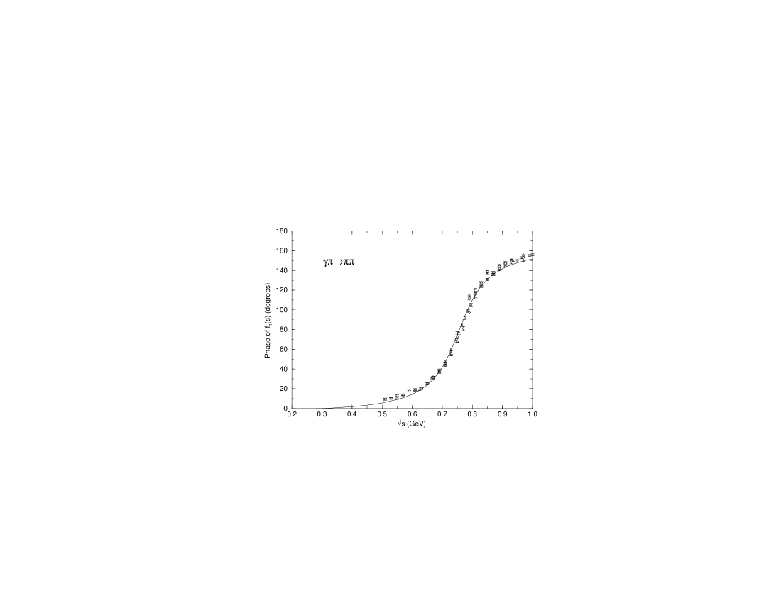
Figure 1: The phase of the lowest partial wave $f_{1}$ obtained from the IAM, Eq. (30), compared to the experimental $\pi\pi$ phase shift $\delta_{1}^{1}$ from Ref. [31] (circles), Ref. [32] (squares), and Ref. [33] (diamonds).

Figure 2: The lowest partial wave $|f_{1}/f_{1}^{(0)}|^{2}$ obtained from the IAM, Eq. (30).

$$\sigma(s)=\frac{24\pi s}{(s-M_{\pi}^{2})^{2}}\frac{M_{\rho}^{2}\Gamma_{\rho}\Gamma_{\pi\gamma}}{(s-M_{\rho}^{2})^{2}+M_{\rho}^{2}\Gamma_{\rho}^{2}}.$$ (33)

Equating the two expressions for the cross section at the resonance energy, the value $\Gamma_{\pi\gamma}=96$ KeV is obtained from the IAM. Experimentally, the value of $\Gamma_{\pi\gamma}$ has been extracted from the production of $\rho$ via the Primakoff effect by incident pion on nuclear targets. The present experimental data are, however, not very consistent with each other [30]. The latest experiment gave the value $\Gamma_{\pi\gamma}=81\pm 4\pm 4$ KeV [34], whereas two earlier experiments gave somewhat lower values for $\Gamma_{\pi\gamma}$ [35]. From the process $e^{+}e^{-}\rightarrow\pi\gamma$, this partial width has also been obtained giving the value $\Gamma_{\pi\gamma}=121\pm 31$ KeV [36]. Therefore, at present it can only be concluded that the value for $\Gamma_{\pi\gamma}$ obtained from the IAM is not in conflict with the experimental situation, but new experiments in the resonance region are definitely needed.

5.2 The full amplitude

If the absorptive part of the higher partial waves with $l\geq 3$ is neglected, it was shown in Sect. 4.1 that the full amplitude could be constructed from the absorptive part of the lowest partial wave. Since the IAM gives a good description of this partial wave up to a least 1 GeV, one may use the absorptive part of this partial wave in the Roy equation for $\gamma\pi\rightarrow\pi\pi$, Eq. (20). With the lowest partial wave approximated by the IAM, the Roy equation may be written with only one subtraction, which is fully determined by the chiral anomaly result. Therefore, the non-perturbative chiral result for the full amplitude can be written as

$$F_{3\pi}(s,t,u)=F_{3\pi}^{(0)}+\frac{1}{\pi}\int_{4M_{\pi}^{2}}^{\infty}ds^{\prime}\frac{{\rm Im}f_{1}(s^{\prime})}{s^{\prime}}\left(\frac{s}{s^{\prime}-s}+\frac{t}{s^{\prime}-t}+\frac{u}{s^{\prime}-u}\right),$$ (34)

where ${\rm Im}f_{1}$ is given by the absorptive part of the IAM result (30). The full amplitude is by construction fully symmetrical in $s$, $t$, and $u$. However, if the lowest partial wave $f_{1}$ is projected out from Eq. (34), the result does not agree exactly with the IAM result (30). This is due to the fact that the left cut is now fully determined from crossing symmetry instead of being approximated by the chiral expansion. In the elastic region below 1 GeV, the difference is, however, negligible. From the full amplitude, Eq. (34), it is also found that the higher partial waves are very small below 1 GeV. Therefore, the cross section can indeed be expressed in terms of $|f_{1}|^{2}$ to a very good approximation. For a somewhat different evaluation of the Roy equation for $\gamma\pi\rightarrow\pi\pi$, see Ref. [37].

As the IAM was derived using elastic unitarity, it is expected that this result is only applicable in the elastic region. The high energy part of the dispersion relation (34) is therefore not expected to be very well approximated by the IAM. Still, at low and moderate energies the dispersion relation should be almost completely saturated by the $\rho$(770) contribution. Therefore, at these energies the high energy part of the dispersion relation should not be very important. Furthermore, at these energies it is also expected that the contribution from the higher partial waves to the Roy equation should be negligible. Therefore, the non-perturbative chiral result (34) should give a rather accurate description of the full amplitude at low and moderate energies. From this result, it is possible to determine the subtraction constants $\bar{C}$ and $\bar{D}$ in the two-loop ChPT result (23) via the sum rules

$$\bar{C}=\frac{1}{F_{3\pi}^{(0)}}\frac{1}{\pi}\int_{4M_{\pi}^{2}}^{\infty}ds^{\prime}\frac{{\rm Im}f_{1}(s^{\prime})}{s^{\prime 2}}\;\;\;\;,\;\;\;\;\bar{D}=\frac{1}{F_{3\pi}^{(0)}}\frac{1}{\pi}\int_{4M_{\pi}^{2}}^{\infty}ds^{\prime}\frac{{\rm Im}f_{1}(s^{\prime})}{s^{\prime 3}}.$$ (35)

Evaluating these sum rules, one obtains the values $\bar{C}=0.93$ ${\rm GeV}^{-2}$ and $\bar{D}=2.12$ ${\rm GeV}^{-4}$, respectively. These sum rules are indeed almost completely saturated by the dispersion relation up to 1 GeV, as the higher energy part only contributes by approximately 2% for $\bar{C}$ and approximately 1% for $\bar{D}$. With the one-loop coupling constant $\bar{c}_{1}$ determined from the assumption of vector resonance saturation, Eq. (31), this gives the following values for the two-loop coupling constants

$$\bar{c}_{2}=-20\;\;\;\;,\;\;\;\;\bar{d}_{2}=2.7.$$ (36)

These values are slightly different from the values determined directly from the IAM (32). As it has already been stated, this is indeed to be expected since the IAM contains higher order unitarity effects, which will effect the determination of these coupling constants.

Another way to combine unitarity and the chiral expansion has been proposed by Holstein [38]. In this model, vector meson dominance is combined with one-loop ChPT in order to account for rescattering effects. Projecting out the lowest partial wave, it is found that unitarity is approximately satisfied and that the $\rho\rightarrow\pi\gamma$ partial width is given by $\Gamma_{\pi\gamma}=84$ KeV. Within this model, one obtains the values

$$\bar{c}_{2}=-19\;\;\;\;,\;\;\;\;\bar{d}_{2}=2.9,$$ (37)

which agree very well with the determination given in (36). However, from the model proposed by Holstein, all higher partial waves have the same phase as the lowest partial wave, which is in contradiction with the experimental facts. In order to remedy this, the lowest partial wave obtained in this model may be inserted in the dispersion relation (34). The resulting amplitude still agrees well with the experimental information, but now implies that all the higher partial waves are real. This gives the values $\bar{c}_{2}=-16$ and $\bar{d}_{2}=2.8$ from the sum rules (35), which is also fully consistent with the values given in (36). Therefore, it seems that the solution of the sum rules is rather robust against small variations of the input.

In the numerical results for two-loop ChPT (23), the values of $\bar{c}_{2}$ and $\bar{d}_{2}$ determined in (36) will be used together with the value of $\bar{c}_{1}$ given in (31). For the low-energy constants $\bar{l}_{1}$ and $\bar{l}_{2}$, these have been determined in ChPT. With the use of the two-loop result for the $\pi\pi$ scattering amplitude and fitting the $D$ partial wave scattering lengths, the value $\bar{l}_{2}-\bar{l}_{1}=6.0$ has been obtained [9]. Similar values have also recently been obtained from a two-loop calculation of the $K_{l4}$ form factors [39]. These values are rather consistent with the value given in (31) but are somewhat lower than the value $\bar{l}_{2}-\bar{l}_{1}=7.8$ obtained from a dispersive improved one-loop calculation of the $K_{l4}$ form factors [40]. However, the numerical result only depends very slightly on the exact value of $\bar{l}_{2}-\bar{l}_{1}$. Therefore, the values given in Eq. (31) for both $\bar{l}_{2}-\bar{l}_{1}$ and $\bar{l}_{4}$ will also be used for ChPT.

6 Numerical results

6.1 Amplitude and cross section

Fig. 3 shows the absolute square of the amplitude normalized to the chiral anomaly. In the sub-threshold region, the two-loop result is rather close to the one-loop result, whereas the corrections start to be of importance slightly above threshold. As for the one-loop result, this gives an almost constant correction to the leading order chiral anomaly result. This is due to the fact that the only variation comes from the $s$, $t$, and $u$ dependency of the function $F$ in the one-loop expression (10). The contribution from the subtraction constants is also shown in the figure, where this contribution is obtained from the expression $F_{3\pi}(s,t,u)=F_{3\pi}^{(0)}[1+\bar{C}(s+t+u)+\bar{D}(s^{2}+t^{2}+u^{2})]$. It is observed that this part gives the main contribution to the two-loop result, which is due to the presence of the $\rho$(770) resonance. However, the unitarity corrections coming from the $U(x)$ terms are also of some importance in the numerical result. In fact, these unitarity corrections are essential in the non-perturbative chiral result, Eq. (34), which is also shown in the figure. The deviation between this result and the two-loop chiral result gives an estimate of the range of validity of the truncated chiral expansion. From this deviation, it is observed that still higher order chiral corrections should begin to be of some importance somewhat around $s=10M_{\pi}^{2}$, which is also observed in other two-loop calculations.

Figure 3: The amplitude $|F_{3\pi}/F_{3\pi}^{(0)}|^{2}$ evaluated at $t=u$ as a function of $s/M_{\pi}^{2}$. The solid line is the two-loop result, Eq. (23), the dashed line the one-loop result, Eq. (10), and the dotted line the leading order chiral anomaly result, Eq. (8). Finally, the long-dashed line is the non-perturbative chiral result, Eq. (34), and the dash-dotted line is the contribution from the subtraction constants.

In Fig. 4, the total cross section is shown as a function of $s/M_{\pi}^{2}$, where the total cross section is given by Eq. (4). Since the one-loop expression for $F_{3\pi}(s,t,u)$ is more or less constant in the whole phase space, the one-loop result for the cross section gives an almost constant correction to the leading order result of approximately 20 %. Close to threshold, the additional two-loop correction is rather small compared to the one-loop correction, whereas this is not the case for higher energies. The additional two-loop correction amounts to approximately 75 % of the one-loop correction at $s=10M_{\pi}^{2}$, and even more at higher energies. This indicates that even higher order terms in the chiral expansion should begin to be of importance at this energy. This is also observed in the figure, where the non-perturbative chiral result begins to deviate from the two-loop result around this energy.

Figure 4: The total cross section as a function of $s/M_{\pi}^{2}$. The solid line is the two-loop result, the dashed line the one-loop result, the dotted line the leading order result and the long-dashed line the non-perturbative chiral result.

6.2 Comparison with experiments

The process $\gamma\pi\rightarrow\pi\pi$ has been investigated at low energies by the Serpukhov experiment [16]. This experiment used the Primakoff reaction of pion pair production by pions in the nuclear Coulomb field

$$\pi^{-}+(Z,A)\rightarrow\pi^{-}+\pi^{0}+(Z,A).$$ (38)

The cross section for this process is related to the $\gamma\pi\rightarrow\pi\pi$ cross section through the equivalent photon method

$$\frac{d\sigma}{dsdtdq^{2}}=\frac{Z^{2}\alpha}{\pi}\left[\frac{q^{2}-q^{2}_{\rm min}}{q^{4}}\right]\frac{1}{s-M^{2}_{\pi}}\frac{d\sigma_{\gamma\pi\rightarrow\pi\pi}}{dt},$$ (39)

where

$$\frac{d\sigma_{\gamma\pi\rightarrow\pi\pi}}{dt}=\frac{|F_{3\pi}(s,t,u)|^{2}}{512\pi}(s-4M^{2}_{\pi})\sin^{2}\theta$$ (40)

and

$$q^{2}_{\rm min}=\left(\frac{s-M^{2}_{\pi}}{2E}\right)^{2}$$ (41)

and $E$ is the energy of the incident pion beam. Neglecting the $q^{2}$ dependency in $F_{3\pi}(s,t,u)$, i.e., setting $q^{2}\approx 0$ so that $s+t+u=3M_{\pi}^{2}$, the total cross section is given by

$$\sigma = \frac{Z^{2}\alpha}{1024\pi^{2}}\int_{4M^{2}_{\pi}}^{s_{\rm max}}ds\frac{(s-4M^{2}_{\pi})^{3/2}}{s^{1/2}}\left[\ln\frac{q^{2}_{\rm max}}{q^{2}_{\rm min}}+\frac{q^{2}_{\rm min}}{q^{2}_{\rm max}}-1\right]\times$$ (42)

$$\int_{0}^{\pi}d\theta\sin^{3}\theta|F_{3\pi}(s,t,u)|^{2}.$$

The Serpukhov experiment was carried out with a 40 GeV pion beam and the maximum momentum transfer was $q^{2}_{\rm max}=2\times 10^{-3}$ ${\rm GeV}^{2}\ll M_{\pi}^{2}$. Thus, the $q^{2}$ dependency in $F_{3\pi}(s,t,u)$ can indeed be neglected when one compares with this experiment.

The kinematical region studied in the Serpukhov experiment was restricted to $s_{\rm max}=10M_{\pi}^{2}$. Three different targets (C, Al, and Fe) were used and the measured total cross sections were found to agree well with the theoretical $Z^{2}$ dependence. Averaging the values of $\sigma/Z^{2}$ obtained from the three different targets, the experimental result given in Table 1 was obtained. This experimental result has to be compared with the theoretical predictions, which are also given in Table 1. It is observed that the two-loop contribution gives a sizable correction to the one-loop result, whereas the further correction from the non-perturbative chiral result is rather small. Nevertheless, all results are still somewhat below the central experimental value, which, however, also has rather large error bars.

Table 1: The total cross section for the Primakoff reaction (38) divided by $Z^{2}$. The theoretical predictions are obtained from Eq. (42) with $F_{3\pi}(s,t,u)$ given by the leading order chiral anomaly result ($O(p^{4})$), the one-loop result ($O(p^{6})$), the two-loop result ($O(p^{8})$), and the non-perturbative chiral result (NPCR). The experimental result is the average value obtained in Ref. [16], where the first (second) error is statistical (systematic).

	$O(p^{4})$	$O(p^{6})$	$O(p^{8})$	NPCR	Experiment
$\sigma/Z^{2}$ (nb)	0.92	1.09	1.18	1.21	$1.63\pm 0.23\pm 0.13$

Table 2: The chiral anomaly $F_{3\pi}^{(0)}$ extracted from the experimental data. The different values correspond to setting $F_{3\pi}(s,t,u)$ in Eq. (42) equal to the leading order chiral anomaly result ($O(p^{4})$), the one-loop result ($O(p^{6})$), the two-loop result ($O(p^{8})$), and the non-perturbative chiral result (NPCR). The theoretical result is from Eq. (8) with $F_{\pi}=92.4\pm 0.3$ MeV [30].

	$O(p^{4})$	$O(p^{6})$	$O(p^{8})$	NPCR	Theory
$F_{3\pi}^{(0)}$ (${\rm GeV}^{-3}$)	$12.9\pm 1.4$	$11.9\pm 1.3$	$11.4\pm 1.3$	$11.3\pm 1.3$	$9.7\pm 0.1$

From the experimental result of $\sigma/Z^{2}$, it is possible to extract the value of the chiral anomaly $F_{3\pi}^{(0)}$, if this is regarded as a free parameter. These extracted values are shown in Table 2, where the statistical and systematic errors have been added. The theoretical prediction obtained from Eq. (8) is also shown in this table. With $F_{3\pi}(s,t,u)$ given by the leading order chiral anomaly result, one obtains a value of $F_{3\pi}^{(0)}$ which is 2.3$\sigma$ too high compared with the theoretical prediction. This result for $F_{3\pi}^{(0)}$ is the value generally quoted from the analysis in Ref. [16]. However, with the one-loop expression for $F_{3\pi}(s,t,u)$, one obtains a value of $F_{3\pi}^{(0)}$ which is only 1.7$\sigma$ too high, and with the two-loop result the disagreement is only at the 1.3$\sigma$ level.

Since the non-perturbative chiral result is close to the two-loop result, the uncertainty coming from yet higher orders in the chiral expansion should be rather small, at least in the kinematical region probed by the Serpukhov experiment. There is of course also some uncertainty due to the uncertainty in the determination of the coupling constants $\bar{c}_{2}$ and $\bar{d}_{2}$. However, as already discussed, this uncertainty should also be rather small. Therefore, in view of the disagreement between the theoretical predictions and the Serpukhov experiment, new improved Primakoff experiments are definitely needed.

The process $\gamma\pi\rightarrow\pi\pi$ has also been investigated at low energies at CERN [41]. This experiment used the reaction $\pi^{-}e\rightarrow\pi^{-}\pi^{0}e$ with 300 GeV pions and measured the total cross section for this process. It was found that the cross section obtained agreed with the chiral anomaly prediction with three number of colors. However, since the error bars were rather large, it was not possible to observe any systematic deviations from the soft pion and soft photon limit in this experiment.

Therefore, new precision experiments are necessary in order to investigate the process $\gamma\pi\rightarrow\pi\pi$ and thus the theory of chiral anomalies in greater detail. Indeed, such new experiments are under way at different facilities. In the COMPASS experiment at CERN [17] and in the SELEX experiment at FNAL (E781) [18], the Primakoff reaction (38) will be measured with 600 and 50-280 GeV pion beams, respectively. In these two experiments, the expected number of near threshold two-pion events is several orders of magnitude higher than previously obtained. This will allow analysis of the data separately in different intervals of $s$ with small statistical errors.

The SELEX experiment will also measure the reaction $\pi^{-}e\rightarrow\pi^{-}\pi^{0}e$ in order to obtain independent information on the $\gamma\pi\rightarrow\pi\pi$ amplitude. For this reaction, the expected number of events is also significantly larger than previously obtained, which would give excellent complementary information on $F_{3\pi}(s,t,u)$.

Finally, at CEBAF the process $\gamma\pi\rightarrow\pi\pi$ is investigated by measuring $\gamma p\rightarrow\pi^{+}\pi^{0}n$ cross sections using tagged photons [19]. Since the resonance region will also be measured in this experiment, this could give new information on the $\rho\rightarrow\pi\gamma$ partial width $\Gamma_{\pi\gamma}$. However, as the incident pion is virtual in the CEBAF experiment, this has to be taken into account when comparing with theory.

7 Conclusion

The anomalous process $\gamma\pi\rightarrow\pi\pi$ plays an important role in the theory of chiral anomalies. At leading order in the chiral expansion, which corresponds to the soft pion and soft photon limit, the amplitude for this process is given in terms of the number of colors $N_{c}$ of the strong interaction. Comparing the leading order result with the present experimental information [16], one finds that the value $N_{c}=4$ is favored.

In order to test this important conclusion more precisely, it is necessary with both experimental and theoretical improvements. Indeed, significant improvements on the experimental side are expected from several new experiments [17, 18, 19]. On the theoretical side, the one-loop correction to the leading order result has previously been calculated [15]. However, in view of the new precision experiments, it is important also to calculate the additional two-loop correction to the amplitude.

This has been the purpose of the present paper, where the amplitude for the anomalous process $\gamma\pi\rightarrow\pi\pi$ has been evaluated to two loops in the chiral expansion by means of a dispersive method. The two new coupling constants that enter at two-loop order were determined from sum rules with the use of a non-perturbative chiral approach. The uncertainty in the numerical results due to this determination was estimated to be rather small. Moreover, the still higher order terms in the chiral expansion were also estimated to be small at low energies.

The two-loop result improves the agreement with the present experimental information [16] compared to both the leading order and the one-loop results. However, the two-loop prediction is still significantly below the central experimental data for $N_{c}=3$. This fact is not likely to be due to theoretical uncertainties. Therefore, should the new experiments [17, 18, 19] confirm the present central experimental value with better precision, it would be a serious problem for QCD.

References

- [1] S. Weinberg, Physica A 96 (1979) 327.
- [2] J. Gasser and H. Leutwyler, Ann. Phys. (N.Y.) 158 (1984) 142.
- [3] J. Gasser and H. Leutwyler, Nucl. Phys. B 250 (1985) 465.
- [4] H. Leutwyler, Ann. Phys. (N.Y.) 235 (1994) 165.
- [5] For some reviews on ChPT see e.g. U. G. Meißner, Rep. Prog. Phys. 56 (1993) 903; A. Pich, Rep. Prog. Phys. 58 (1995) 563; G. Ecker, Prog. Part. Nucl. Phys. 35 (1995) 1; J. Bijnens and U. G. Meißner, Proc. Workshop on Chiral Effective Theories, Bad Honnef, Germany, 30 November - 4 December 1998 (hep-ph/9901381).
- [6] J. Gasser and U. G. Meißner, Nucl. Phys. B 357 (1991) 90; G. Colangelo, M. Finkemeier and R. Urech, Phys. Rev. D 54 (1996) 4403.
- [7] J. Bijnens, G. Colangelo and P. Talavera, JHEP 05 (1998) 014.
- [8] M. Knecht et al., Nucl. Phys. B 457 (1995) 513.
- [9] J. Bijnens et al., Phys. Lett. B 374 (1996) 210; Nucl. Phys. B 508 (1997) 263; 517 (1998) 639 (E).
- [10] S. Bellucci, J. Gasser and M. E. Sainio, Nucl. Phys. B 423 (1994) 80; B 431 (1994) 413 (E); U. Bürgi, Phys. Lett. B 377 (1996) 147; Nucl. Phys. B 479 (1996) 392; J. Bijnens and P. Talavera, Nucl. Phys. B 489 (1997) 387.
- [11] J. Wess and B. Zumino, Phys. Lett. 37 B (1971) 95; E. Witten, Nucl. Phys. B 223 (1983) 422.
- [12] J. Bijnens, A. Bramon and F. Cornet, Z. Phys. C 46 (1990) 599; D. Issler, preprint SLAC-PUB-4943; R. Akhoury and A. Alfakih, Ann. Phys. (N.Y.) 210 (1991) 81; H. W. Fearing and S. Scherer, Phys. Rev. D 53 (1996) 315.
- [13] For a review on ChPT in the anomalous sector see J. Bijnens, Int. J. Mod. Phys. A 8 (1993) 3045.
- [14] S. L. Adler et al., Phys. Rev. D 4 (1971) 3497; M. V. Terent’ev, Phys. Lett. 38 B (1972) 419; R. Aviv and A. Zee, Phys. Rev. D 5 (1972) 2372.
- [15] J. Bijnens, A. Bramon and F. Cornet, Phys. Lett. B 237 (1990) 488.
- [16] Yu. M. Antipov et al., Phys. Rev. D 36 (1987) 21.
- [17] M. A. Moinester, V. Steiner and S. Prakhov, in Proc. XXXVII Int. Winter Meeting on Nuclear Physics, Bormio, Italy, 25 - 29 January 1999, ed. I. Iori (Ricerca Scientifica ed Educazione Permanente Supplemento No. 114, 1999), preprint TAUP-2562-99 (hep-ex/9903017).
- [18] SELEX Collaboration, M. A. Moinester et al., in Proc. 8th Int. Conf. on the Structure of Baryons (BARYONS ’98), Bonn, Germany, 22 - 26 September 1998, eds. D. W. Menze and B. Metsch (World Scientific, Singapore, 1999), preprint TAUP-2568-99 (hep-ex/9903039); M. A. Moinester, in Proc. Int. Conf. on Physics with GeV Particle Beams, Jülich, Germany, 22 - 25 August 1994, eds. H. Machner and K. Sistemich (World Scientific, N.J., 1994), preprint TAUP-2176-94 (hep-ph/9409307).
- [19] R. A. Miskimen, K. Wang and A. Yegneswaran, Spokesmen, CEBAF Proposal PR-94-015, 1994.
- [20] K. M. Watson, Phys. Rev. 95 (1954) 228.
- [21] S. L. Adler, Phys. Rev. 177 (1969) 2426; J. S. Bell and R. Jackiw, Nuovo Cimento A 60 (1969) 47; W. A. Bardeen, Phys. Rev. 184 (1969) 1848.
- [22] J. F. Donoghue, B. R. Holstein and Y. C. R. Lin, Phys. Rev. Lett. 55 (1985) 2766; J. Bijnens, A. Bramon and F. Cornet, Phys. Rev. Lett. 61 (1988) 1453.
- [23] G. Ecker et al., Nucl. Phys. B 321 (1989) 311; G. Ecker et al., Phys. Lett. B 223 (1989) 425.
- [24] S. M. Roy, Phys. Lett. 36 B (1971) 353; J. L. Basdevant, J. C. Le Guillou and H. Navelet, Nuovo Cimento 7 A (1972) 363; J. L. Petersen, CERN Yellow Report, CERN 77-04.
- [25] J. Stern, H. Sazdjian and N. H. Fuchs, Phys. Rev. D 47 (1993) 3814.
- [26] T. N. Truong, Phys. Rev. Lett. 61 (1988) 2526; 67 (1991) 2260.
- [27] A. Dobado and J. R. Peláez, Phys. Rev. D 47 (1993) 4883; 56 (1997) 3057; T. Hannah, Phys. Rev. D 51 (1995) 103; 52 (1995) 4971; 54 (1996) 4648.
- [28] T. Hannah, Phys. Rev. D 55 (1997) 5613.
- [29] J. A. Oller, E. Oset and J. R. Peláez, Phys. Rev. Lett. 80 (1998) 3452; Phys. Rev. D 59 (1999) 074001; 60 (1999) 099906 (E); F. Guerrero and J. A. Oller, Nucl. Phys. B 537 (1999) 459.
- [30] Particle Data Group, C. Caso et al., Eur. Phys. J. C 3 (1998) 1.
- [31] P. Estabrooks and A. D. Martin, Nucl. Phys. B 79 (1974) 301.
- [32] S. D. Protopopescu et al., Phys. Rev. D 7 (1973) 1279.
- [33] B. Hyams et al., Nucl. Phys. B 64 (1973) 134; W. Ochs, Ph.D. thesis, Ludwig-Maximilians-Universität, 1973.
- [34] L. Capraro et al., Nucl. Phys. B 288 (1987) 659.
- [35] J. Huston et al., Phys. Rev. D 33 (1986) 3199; T. Jensen et al., Phys. Rev. D 27 (1983) 26.
- [36] S. I. Dolinsky et al., Z. Phys. C 42 (1989) 511.
- [37] T. N. Truong, in Proc. 4th Workshop on Quantum Chromodynamics, Paris, France, 1 - 6 June 1998, eds. H. M. Fried and B. Mueller (World Scientific, Singapore, 1999) (hep-ph/9903378).
- [38] B. R. Holstein, Phys. Rev. D 53 (1996) 4099.
- [39] G. Amorós, J. Bijnens and P. Talavera, Phys. Lett. B 480 (2000) 71; Nucl. Phys. B 585 (2000) 293.
- [40] J. Bijnens, G. Colangelo and J. Gasser, Nucl. Phys. B427 (1994) 427.
- [41] S. R. Amendolia et al., Phys. Lett. 155 B (1985) 457.