Abstract

We present a comprehensive analysis of the sensitivity of the TESLA $e^{+}e^{-}$ collider to top flavour-changing neutral couplings to the $Z$ boson and photon. We study single top production and top decay processes, and we consider the cases without beam polarization, with only $e^{-}$ polarization and with $e^{-}$ and $e^{+}$ polarization. We show that the use of the latter substantially enhances the sensitivity to discover or bound these vertices, and for some of the couplings the expected LHC limits could be improved by factors $2-14$ for equal running times.

1 Introduction

It is generally believed that the top quark, because of its large mass, will be a sensitive probe into physics beyond the Standard Model (SM) [1]. In particular, its couplings to the gauge and Higgs bosons may show deviations with respect to the SM predictions. In the SM the flavour-changing neutral (FCN) couplings $Ztq$, with $q=u,c$, vanish at tree-level by the GIM mechanism, and the $\gamma tq$ and $gtq$ ones are zero as a consequence of the unbroken ${\mathrm{S}U(3)}_{c}\times{\mathrm{U}(1)}_{Q}$ symmetry. The $Htq$ couplings also vanish due to the existence of only one Higgs doublet. These types of vertices can be generated at the one-loop level, but they are very suppressed by the GIM mechanism, because the masses of the charge $-1/3$ quarks in the loop are small compared to the scale involved. The single top production branching may be estimated roughly by $\mathrm{Br}(Z\to tc)=1.5\times 10^{-13}$ [2], and the calculation of the branching ratios for top decays mediated by these FCN operators yields the SM predictions $\mathrm{Br}(t\to Zc)=1.3\times 10^{-13}$, $\mathrm{Br}(t\to\gamma c)=4.5\times 10^{-13}$, $\mathrm{Br}(t\to gc)=3.5\times 10^{-11}$ [3], $\mathrm{Br}(t\to Hc)=3.5\times 10^{-14}$ [4] , and smaller values for the up quark. However, in many simple SM extensions these rates can be orders of magnitude larger. For instance, in models with exotic quarks $\mathrm{Br}(t\to Zq)$ can be of order $10^{-3}-10^{-2}$ [5]. Two Higgs doublet models allow for $\mathrm{Br}(t\to Zc)=10^{-6}$, $\mathrm{Br}(t\to\gamma c)=10^{-7}$, $\mathrm{Br}(t\to gc)=10^{-4}$ [6], and in $R$ parity-violating supersymmetric models one can have $\mathrm{Br}(t\to Zc)=10^{-4}$, $\mathrm{Br}(t\to\gamma c)=10^{-5}$, $\mathrm{Br}(t\to gc)=10^{-3}$ [7]. Top FCN decays into a light Higgs boson and an up or charm quark can also have similar or larger rates in models with exotic quarks [8, 5], with more than one Higgs doublet [6, 9] or with supersymmetry [10]. Hence, top FCN couplings offer a good place to search for new physics, which may manifest if these vertices are observed in future colliders. In addition, the study of FCN couplings provides model-independent information on the charged current couplings and the unitarity of the CKM matrix [11]. Here we will focus on FCN interactions involving the top, a light charge $2/3$ quark $q$ and a neutral gauge boson $V=Z,\gamma$. At present the best limits on $Ztq$ couplings come from LEP 2, $\mathrm{Br}(t\to Zq)\leq 0.07$ [12, 13], and the best limits on $\gamma tq$ couplings from Tevatron, $\mathrm{Br}(t\to\gamma q)\leq 0.032$ [14]. They are very weak but will improve in the next years, first with Tevatron Run II, and later with the next generation of colliders.

The CERN LHC will be a top factory. With a $t\bar{t}$ production cross-section of 830 pb, at its 100 fb^-1 luminosity phase it will produce $8.3\times 10^{7}$ top-antitop pairs per year. In addition, it will produce $3\times 10^{7}$ single tops plus antitops via other processes [15, 16]. This makes LHC an excellent machine for the investigation of the top quark properties. The search for FCN top couplings can be carried out examining two different types of processes. On the one hand, we can look for rare top decays $t\to Zq$ [17], $t\to\gamma q$ [18], $t\to gq$ [19] or $t\to Hq$ [20] of the tops or antitops produced in the SM process $gg,q\bar{q}\to t\bar{t}$. On the other hand, one can search for single top production via an anomalous effective vertex: $Zt$ and $\gamma t$ production [21], the production of a top quark without or with a light jet [22, 23], and $Ht$ production [20]. In these cases the top quark is assumed to decay in the SM dominant mode $t\to Wb$. One can also search for like-sign $tt$ production [24] and other exotic processes.

The TESLA $e^{+}e^{-}$ collider with a centre of mass (CM) energy of $\sqrt{s}=500$ GeV has a tree-level $t\bar{t}$ production cross-section of 0.52 pb, and produces only $1.56\times 10^{5}$ top-antitop pairs per year with its expected luminosity of 300 fb^-1. However, $e^{+}e^{-}$ colliders are cleaner than hadron colliders. For instance, the signal to background ratio $S/B$ for rare top decays can be 7 times larger in TESLA than in LHC. But the sensitivity to rare top decays is given in the Gaussian statistics limit by the ratio $S/\sqrt{B}$, and the larger LHC cross-sections make difficult for TESLA to compete with it in the search for anomalous top couplings.

In this paper we show that the use of beam polarization in TESLA substantially enhances its sensitivity to discover or bound top anomalous FCN couplings and allows to improve some of the expected LHC limits up to an order of magnitude [25]. We first study the single top production process $e^{+}e^{-}\to t\bar{q}$, mediated by $Ztq$ or $\gamma tq$ anomalous couplings [26]. Then we study rare top decays in the processes $e^{+}e^{-}\to t\bar{t}$, with subsequent decay $\bar{t}\to V\bar{q}$. In all cases we take into account the charge conjugate processes as well: we sum $t\bar{q}+\bar{t}q$ production, and we consider $\bar{t}\to V\bar{q}$ or $t\to Vq$. Single top production and top decay processes are complementary. Single top production is more sensitive to top anomalous couplings but top decays can help to disentangle the type of anomalous coupling involved ($Ztq$ or $\gamma tq$) if a positive signal is discovered.

We consider the planned CM energies of 500 and 800 GeV, and for both we analyse the cases: (i) without beam polarization, (ii) with $80\%$ $e^{-}$ polarization, and (iii) with $80\%$ $e^{-}$, $45\%$ $e^{+}$ polarization. The paper is organized as follows. In Section 2 we describe the procedure used to compute the signals and backgrounds and to obtain the limits. In Section 3 we analyse single top production. In Sections 4 and 5 we consider top decays $t\to\gamma q$ and $t\to Zq$, respectively. In Section 6 we summarize the results and draw our conclusions.

2 Generation of signals and backgrounds

In order to describe the FCN couplings among the top, a light quark $q$ and a $Z$ boson or a photon $A$ we use the Lagrangian

$$-{\mathcal{L}} = \frac{g_{W}}{2c_{W}}\,X_{tq}\,\bar{t}\gamma_{\mu}(x_{tq}^{L}P_{L}+x_{tq}^{R}P_{R})qZ^{\mu}+\frac{g_{W}}{2c_{W}}\,\kappa_{tq}\,\bar{t}(\kappa_{tq}^{v}-\kappa_{tq}^{a}\gamma_{5})\frac{i\sigma_{\mu\nu}q^{\nu}}{m_{t}}qZ^{\mu}$$ (1)

$$+e\,\lambda_{tq}\,\bar{t}(\lambda_{tq}^{v}-\lambda_{tq}^{a}\gamma_{5})\frac{i\sigma_{\mu\nu}q^{\nu}}{m_{t}}qA^{\mu}\,,$$

where $P_{R,L}=(1\pm\gamma_{5})/2$. The chirality-dependent parts are normalized to $(x_{tq}^{L})^{2}+(x_{tq}^{R})^{2}=1$, $(\kappa_{tq}^{v})^{2}+(\kappa_{tq}^{a})^{2}=1$, $(\lambda_{tq}^{v})^{2}+(\lambda_{tq}^{a})^{2}=1$. This effective Lagrangian contains $\gamma_{\mu}$ terms of dimension 4 and $\sigma_{\mu\nu}$ terms of dimension 5. The couplings are constants corresponding to the first terms in the expansion in momenta. The $\sigma_{\mu\nu}$ terms are the only ones allowed by the unbroken gauge symmetry, ${\mathrm{S}U(3)}_{c}\times{\mathrm{U}(1)}_{Q}$. Due to their extra momentum factor they grow with the energy and make large colliders the best places to measure them.

For single top production we study the process $e^{+}e^{-}\to t\bar{q}$ mediated by $Ztq$ or $\gamma tq$ anomalous couplings (see Fig. 1). We will only take one anomalous coupling different from zero at the same time. However, if a positive signal is discovered, it may be difficult to distinguish only from this process whether the anomalous coupling involves the $Z$ boson, the photon or both. On the other hand, in principle it could be possible to have a fine-tuned cancellation between $Z$ and $\gamma$ contributions that led to a suppression of this signal.

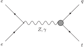
Figure 1: Feynman diagrams for $e^{+}e^{-}\to t\bar{q}$ via $Ztq$ or $\gamma tq$ FCN couplings. The top quark is off-shell and has the SM decay.

For top decays we study the SM process $e^{+}e^{-}\to t\bar{t}$, followed by antitop decay mediated by an anomalous $Ztq$ or $\gamma tq$ coupling (see Fig. 2). This gives the signals $t\bar{q}Z$ and $t\bar{q}\gamma$, and the observation of the final state distinguishes $Ztq$ and $\gamma tq$ couplings. In the $t\bar{q}$, $t\bar{q}Z$ and $t\bar{q}\gamma$ signals the top is assumed to decay via $t\to W^{+}b\to l^{+}\nu b$, with $l=e,\mu$. For the $t\bar{q}Z$ signal we only consider the $Z$ boson decays to electrons and muons.

   

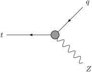
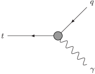
Figure 2: Feynman diagrams for FCN antitop decay via $Ztq$ or $\gamma tq$ FCN couplings.

For the $t\bar{q}$ signal we calculate the matrix element $e^{+}e^{-}\to t\bar{q}\to W^{+}b\bar{q}\to l^{+}\nu b\bar{q}$. For the $t\bar{q}Z$ and $t\bar{q}\gamma$ signals we calculate $e^{+}e^{-}\to t\bar{t}\to W^{+}b\bar{q}Z\to l^{+}\nu b\bar{q}l^{\prime+}l^{\prime-}$ and $e^{+}e^{-}\to t\bar{t}\to W^{+}b\bar{q}\gamma\to l^{+}\nu b\bar{q}\gamma$, respectively. These matrix elements are evaluated using HELAS [27] and introducing a new HELAS-like subroutine IOV2XX to compute the non-renormalizable $\sigma_{\mu\nu}$ vertex. This new routine has been checked by hand. In all cases we sum the contribution of the charge conjugate processes. For the $t\bar{q}V$ signals there is an additional contribution from $t\bar{q}$ production plus radiative emission of a $Z$ boson or a photon. This correction is suppressed because it does not have the enhancement due to the $\bar{t}$ on-shell, and is even smaller after the kinematical cuts for the signal reconstruction.

The background for the $t\bar{q}$ signal is given by $W^{+}q\bar{q}^{\prime}$ production with $W^{+}$ decay to electrons and muons. The leading contribution to this process is $W^{+}W^{-}$ production with $W^{-}$ hadronic decay, but it is crucial for the correct evaluation of the background after kinematical cuts to take into account the 7 interfering Feynman diagrams for $e^{+}e^{-}\to W^{+}q\bar{q}^{\prime}$. Taking all the interfering diagrams for $e^{+}e^{-}\to l^{+}\nu q\bar{q}^{\prime}$ into account does not make any appreciable change in the cross-section. The backgrounds for the $t\bar{q}Z$ and $t\bar{q}\gamma$ signals are analogous, $W^{+}q\bar{q}^{\prime}Z$ and $W^{+}q\bar{q}^{\prime}\gamma$, with 46 and 44 diagrams, respectively. These three backgrounds are evaluated using MadGraph [28] and modifying the code to include the $W^{+}$ decay.

To simulate the calorimeter energy resolution we perform a Gaussian smearing of the charged lepton ($l$), photon ($\gamma$) and jet ($j$) energies using a realistic calorimeter resolution [29] of

$$\frac{\Delta E^{l,\gamma}}{E^{l,\gamma}}=\frac{10\%}{\sqrt{E^{l,\gamma}}}\oplus 1\%\,,~{}~{}~{}~{}\frac{\Delta E^{j}}{E^{j}}=\frac{50\%}{\sqrt{E^{j}}}\oplus 4\%\,,$$ (2)

where the energies are in GeV and the two terms are added in quadrature. For simplicity we assume that the energy smearing for muons is the same as for electrons. Note that more optimistic resolutions would improve our results. We then apply detector cuts on transverse momenta $p_{T}$ and pseudorapidities $\eta$

$$p_{T}\geq 10~{}\mathrm{GeV}~{},~{}~{}|\eta|\leq 2.5\,.$$ (3)

The cut on pseudorapidity corresponds to a polar angle $10^{\circ}\leq\theta\leq 170^{\circ}$. We reject the events in which the jets and/or leptons are not isolated, requiring that the distances in $(\eta,\phi)$ space $\Delta R$ satisfy $\Delta R\geq 0.4$. We do not require specific trigger conditions, and we assume that the presence of high $p_{T}$ charged leptons will suffice.

After signal and background reconstruction, which will be analysed in detail for each of the processes discussed, we require a $b$ tag on the jet associated to the decay of the top quark to reduce the backgrounds. We require the $b$ tagged jet to have $|\eta_{b}|\leq 2$ (polar angle $15^{\circ}\leq\theta_{b}\leq 165^{\circ}$) and energy $E_{b}\geq 45$ GeV. We assume a $b$ tagging efficiency of $60\%$, and mistagging rates of $5\%$ for charm and $0.5\%$ for lighter quarks [30]. These are average numbers appropriate for the $E_{b}$ kinematical distributions we will obtain later.

After kinematical cuts, for each of the cases studied we obtain two types of limits on the anomalous coupling parameters $X_{tq}$, $\kappa_{tq}$, $\lambda_{tq}$. Below we outline the procedure used. The correct statistical treatment of signals and backgrounds is specially necessary in our study since the backgrounds are very small, sometimes much less than one event even for high integrated luminosities.

Assuming that no signal is observed after the experiment is done, i.e. the number of observed events $n_{0}$ equals the expected background $n_{b}$, we derive $95\%$ confidence level (CL) upper bounds on the number of events expected $n_{s}$. We use the Feldman-Cousins construction for the confidence intervals of a Poisson variable [31] evaluated with the PCI package [32].

On the other hand, we can obtain the smallest value of $n_{s}$ such that a positive signal is expected to be observed with $3\,\sigma$ significance, assuming that the number of observed events for $3\,\sigma$ ‘evidence’ $n_{e}$ equals $n_{s}+n_{b}$. For a large number of background events, the Poisson probability distribution can be approximated by a Gaussian of mean $n_{b}$ and standard deviation $\sqrt{n}_{b}$. The requirement of $3\,\sigma$ significance is then simply $n_{s}/\sqrt{n}_{b}\geq 3$. However, this is seldom the case for our study, where the backgrounds are very small. In such case, we use the estimator based on the $\mathcal{P}$ number (see for example [33]). The number $\mathcal{P}(n)$ is defined as the probability of the background to fluctuate and give $n$ or more observed events. $n_{e}$ is then defined as the smallest value of $n$ such that $1-\mathcal{P}(n)\geq 99.73\%$, corresponding to three Gaussian standard deviations.

Another possible estimator for the evidence of a signal can be built using Feldman-Cousins intervals. For a fixed value of $n_{b}$, we define the number of observed events for $3\,\sigma$ evidence $n_{e}$ as the smallest value of the number of observed events $n$ such that the $99.73\%$ CL Feldman-Cousins intervals do not contain zero. These two estimators for the evidence of a signal can be shown to be equivalent, and for $n_{b}\geq 9$ both give similar results to the Gaussian approximation $n_{s}/\sqrt{n}_{b}\geq 3$.

In our analysis we find that usually $3\,\sigma$ evidence limits are numerically larger than $95\%$ upper limits, but this is not always the case. For very small backgrounds $3\,\sigma$ limits are smaller, what means that the potential to discover a new signal is better than the ability to set upper bounds on it if nothing is seen. This behaviour can exhibit fluctuations resulting from the discreteness of Poisson statistics, but in general and comparing with LHC, the TESLA discovery potential is better than the potential to set upper limits.

3 Single top production $e^{+}e^{-}\to t\bar{q}$

The process $e^{+}e^{-}\to t\bar{q}$ gives better limits on the top anomalous couplings than top decays. However, it has the disadvantage that the final state $l^{+}\nu bj$ does not distinguish the type of coupling involved. The background is $W^{+}jj$ production with $W^{+}\to l^{+}\nu$ and a jet misidentified as a $b$.

We take only one type of FCN couplings different from zero at the same time, and we evaluate three signals: (i) with $Ztq$ $\gamma_{\mu}$, (ii) with $Ztq$ $\sigma_{\mu\nu}$, and (iii) with $\gamma tq$ couplings. Their cross-sections depend slightly on the chirality of the anomalous couplings. The chirality-dependent parts can be written as $(v-a\,\gamma_{5})$, with $v^{2}+a^{2}=1$. For definiteness, we set $v=1$, $a=0$ in our evaluations. The results are the same setting $v=0$ and $a=1$. For a CM energy of 500 GeV and the three polarization options discussed the cross-section for $\gamma_{\mu}$ couplings differs $\mp 1\%$ setting $v=\pm a=1/\sqrt{2}$, and for $\sigma_{\mu\nu}$ couplings it differs $\pm 1.2\%$.

The signals are reconstructed as follows. The neutrino momentum $p_{\nu}$ can be identified with the missing momentum of the event. The longitudinal missing momentum can also be used, and $p_{\nu}$ is reconstructed without any ambiguity. The $W^{+}$ momentum is then the sum of the momenta of the charged lepton and the neutrino. In the case of $t\bar{q}$ production, the invariant mass of the $W^{+}$ and one of the jets, $m_{t}^{\mathrm{rec}}$, is consistent with the top mass, and the other jet has an energy $E_{q}$ around $E_{q}^{0}\equiv(s-m_{t}^{2})/(2\sqrt{s})$. Of the two possible pairings, we choose the one minimizing $(m_{t}^{\mathrm{rec}}-m_{t})^{2}+(E_{q}-E_{q}^{0})^{2}$ and require a $b$ tag on the jet associated to the top quark. The kinematical distributions for $m_{t}^{\mathrm{rec}}$ and $E_{q}$ for the signals and the background at a CM energy of 500 GeV without beam polarization are plotted in Figs. 3 and 4. The $E_{b}$ distribution is shown in Fig. 5.

Another interesting variable to distinguish the signals from the background is the two-jet invariant mass $M_{W^{-}}^{\mathrm{rec}}$. The $W^{+}jj$ background is dominated by $W^{+}W^{-}$ production with $W^{-}\to jj$, and the $M_{W^{-}}^{\mathrm{rec}}$ distribution peaks around $M_{W}$, as can be clearly seen in Fig. 6. A veto cut on $M_{W^{-}}^{\mathrm{rec}}$ can eliminate a large fraction of the background but makes compulsory to calculate correctly the cross-section to include all the diagrams for $e^{+}e^{-}\to W^{+}q\bar{q}^{\prime}$. Also of interest are the total transverse energy $H_{T}$ and the charged lepton energy $E_{l}$ in Figs. 7 and 8. The kinematical distributions with polarized beams are very similar except the $H_{T}$ distribution. In this case polarization decreases the peak of the background around $H_{T}=200$.

To enhance the signal significance we perform kinematical cuts on these variables. However, we find that the veto cut on $M_{W^{-}}^{\mathrm{rec}}$ is unnecessary in single top production since the requirement $E_{b}>45$ GeV and the kinematical cut on $m_{t}^{\mathrm{rec}}$ practically eliminate the peak in the $M_{W^{-}}^{\mathrm{rec}}$ distribution. A cut on $E_{q}$ is unnecessary because this variable is kinematically related to $m_{t}^{\mathrm{rec}}$, and we prefer to apply a cut on $m_{t}^{\mathrm{rec}}$ to show the presence of a top quark in the signal. For simplicity, we choose to apply the same cuts for the three signals and the three polarization options, but different for CM energies of 500 and 800 GeV. We choose the cuts trying to maintain the independence of the cross-section on the chirality of the coupling. Obviously, our results could be improved modifying the cuts for each type of coupling and each polarization option. We now discuss the results for 500 GeV and 800 GeV in turn.

3.1 Limits at 500 GeV

The kinematical cuts for 500 GeV are collected in Table 1, and the cross-sections before and after cuts for the three polarization options in Table 2. We normalize the signals to $X_{tq}=0.06$, $\kappa_{tq}=0.02$, $\lambda_{tq}=0.02$ and sum the charge conjugate processes. For the chiralities with $v=\pm a$ the cross-section after cuts differs $\pm 6.8\%$ for $\gamma_{\mu}$ couplings and $\mp 4.6\%$ for $\sigma_{\mu\nu}$ couplings.

Variable	500 GeV cut
$m_{t}^{\mathrm{rec}}$	160–190
$H_{T}$	$>220$
$E_{l}$	$<160$

Table 1: Kinematical cuts for the three $t\bar{q}$ signals and the three polarization options at a CM energy of 500 GeV. The masses and the energies are in GeV.

	No pol.		Pol. $e^{-}$		Pol. $e^{-}$ $e^{+}$
	before	after	before	after	before	after
	cuts	cuts	cuts	cuts	cuts	cuts
$t\bar{q}+\bar{t}q$ $(Z,\gamma_{\mu})$	0.183	0.137	0.162	0.121	0.215	0.161
$t\bar{q}+\bar{t}q$ $(Z,\sigma_{\mu\nu})$	0.199	0.153	0.176	0.135	0.234	0.179
$t\bar{q}+\bar{t}q$ $(\gamma)$	0.375	0.288	0.375	0.287	0.510	0.391
$W^{\pm}jj$	19.5	0.0734	4.06	0.0154	2.40	0.0092

Table 2: Cross-sections (in fb) before and after the kinematical cuts in Table 1 for the three $t\bar{q}$ signals and their background at a CM energy of 500 GeV, for the three polarization options. We include $b$ tagging efficiencies and use $X_{tq}=0.06$, $\kappa_{tq}=0.02$, $\lambda_{tq}=0.02$.

We notice in Table 2 the usefulness of polarization: $e^{-}$ polarization decreases the background by a factor of 5, without affecting too much the signals. $e^{+}$ polarization further decreases the background and even increases the cross-section of the signals with respect to the values without polarization.

We express the limits on the anomalous couplings in terms of top decay branching ratios, using $\Gamma_{t}=1.56$ GeV. As explained in the previous Section, we obtain $95\%$ CL upper limits for the case that nothing is observed and $3\,\sigma$ discovery limits. Since the number of background events is small, the limits do not scale with the luminosity $L$ as $1/\sqrt{L}$. In Table 3 we quote limits for a reference integrated luminosity of 100 fb^-1 for comparison with other processes, and in Table 4 for 300 fb^-1, corresponding to one year of operation with the expected luminosity.

	No pol.		Pol. $e^{-}$		Pol. $e^{-}$ $e^{+}$
	$95\%$	$3\,\sigma$	$95\%$	$3\,\sigma$	$95\%$	$3\,\sigma$
$\mathrm{Br}(t\to Zq)$ $(\gamma_{\mu})$	$7.9\times 10^{-4}$	$1.2\times 10^{-3}$	$7.1\times 10^{-4}$	$7.5\times 10^{-4}$	$4.4\times 10^{-4}$	$4.2\times 10^{-4}$
$\mathrm{Br}(t\to Zq)$ $(\sigma_{\mu\nu})$	$6.3\times 10^{-5}$	$9.4\times 10^{-5}$	$5.7\times 10^{-5}$	$6.0\times 10^{-5}$	$3.5\times 10^{-5}$	$3.4\times 10^{-5}$
$\mathrm{Br}(t\to\gamma q)$	$3.9\times 10^{-5}$	$5.9\times 10^{-5}$	$3.2\times 10^{-5}$	$3.3\times 10^{-5}$	$1.9\times 10^{-5}$	$1.8\times 10^{-5}$

Table 3: Limits on top FCN decays obtained from single top production at 500 GeV with a reference luminosity of 100 fb^-1 for the three polarization options.

	No pol.		Pol. $e^{-}$		Pol. $e^{-}$ $e^{+}$
	$95\%$	$3\,\sigma$	$95\%$	$3\,\sigma$	$95\%$	$3\,\sigma$
$\mathrm{Br}(t\to Zq)$ $(\gamma_{\mu})$	$4.4\times 10^{-4}$	$6.1\times 10^{-4}$	$3.1\times 10^{-4}$	$3.9\times 10^{-4}$	$1.9\times 10^{-4}$	$2.2\times 10^{-4}$
$\mathrm{Br}(t\to Zq)$ $(\sigma_{\mu\nu})$	$3.5\times 10^{-5}$	$4.8\times 10^{-5}$	$2.4\times 10^{-5}$	$3.1\times 10^{-5}$	$1.5\times 10^{-5}$	$1.7\times 10^{-5}$
$\mathrm{Br}(t\to\gamma q)$	$2.2\times 10^{-5}$	$3.0\times 10^{-5}$	$1.3\times 10^{-5}$	$1.7\times 10^{-5}$	$8.2\times 10^{-6}$	$9.3\times 10^{-6}$

Table 4: Limits on top FCN decays obtained from single top production at 500 GeV with a luminosity of 300 fb^-1 for the three polarization options.

3.2 Limits at 800 GeV

We write the kinematical cuts for 800 GeV in Table 5, and the cross-sections before and after cuts in in Table 6. We normalize the signals to $X_{tq}=0.06$, $\kappa_{tq}=0.02$, $\lambda_{tq}=0.02$ and sum the charge conjugate processes. The signal cross-sections with non-renormalizable couplings do not decrease going from 500 to 800 GeV, whereas the background decreases by a factor of 2.3. This improves the sensitivity for $\sigma_{\mu\nu}$ couplings with respect to 500 GeV. Unfortunately, the signal with $\gamma_{\mu}$ couplings also decreases, and thus the results are worse in this case. Again we observe the usefulness of polarization: using only $e^{-}$ polarization reduces the background 5 times and using $e^{+}$ polarization as well reduces it 8 times. In Table 7 we gather the limits for a reference integrated luminosity of 100 fb^-1 and in Table 8 for 500 fb^-1, collected in one year with the expected luminosity.

Variable	800 GeV cut
$m_{t}^{\mathrm{rec}}$	160–190
$H_{T}$	$>450$
$E_{l}$	$<300$

Table 5: Kinematical cuts for the three $t\bar{q}$ signals and the three polarization options at a CM energy of 800 GeV. The masses and the energies are in GeV.

	No pol.		Pol. $e^{-}$		Pol. $e^{-}$ $e^{+}$
	before	after	before	after	before	after
	cuts	cuts	cuts	cuts	cuts	cuts
$t\bar{q}+\bar{t}q$ $(Z,\gamma_{\mu})$	0.0776	0.0498	0.0684	0.0440	0.0912	0.0586
$t\bar{q}+\bar{t}q$ $(Z,\sigma_{\mu\nu})$	0.198	0.149	0.175	0.132	0.233	0.175
$t\bar{q}+\bar{t}q$ $(\gamma)$	0.389	0.293	0.389	0.293	0.528	0.398
$W^{\pm}jj$	8.45	0.0125	1.75	0.0028	1.03	0.0018

Table 6: Cross-sections (in fb) before and after the kinematical cuts in Table 5 for the three $t\bar{q}$ signals and their background at a CM energy of 800 GeV, for the three polarization options. We include $b$ tagging efficiencies and use $X_{tq}=0.06$, $\kappa_{tq}=0.02$, $\lambda_{tq}=0.02$.

	No pol.		Pol. $e^{-}$		Pol. $e^{-}$ $e^{+}$
	$95\%$	$3\,\sigma$	$95\%$	$3\,\sigma$	$95\%$	$3\,\sigma$
$\mathrm{Br}(t\to Zq)$ $(\gamma_{\mu})$	$1.3\times 10^{-3}$	$1.6\times 10^{-3}$	$1.1\times 10^{-3}$	$1.4\times 10^{-3}$	$8.3\times 10^{-4}$	$8.0\times 10^{-4}$
$\mathrm{Br}(t\to Zq)$ $(\sigma_{\mu\nu})$	$3.9\times 10^{-5}$	$4.7\times 10^{-5}$	$3.2\times 10^{-5}$	$4.2\times 10^{-5}$	$2.5\times 10^{-5}$	$2.4\times 10^{-5}$
$\mathrm{Br}(t\to\gamma q)$	$2.3\times 10^{-5}$	$2.8\times 10^{-5}$	$1.7\times 10^{-5}$	$2.2\times 10^{-5}$	$1.3\times 10^{-5}$	$1.2\times 10^{-5}$

Table 7: Limits on top FCN decays obtained from single top production at 800 GeV with a reference luminosity of 100 fb^-1 for the three polarization options.

	No pol.		Pol. $e^{-}$		Pol. $e^{-}$ $e^{+}$
	$95\%$	$3\,\sigma$	$95\%$	$3\,\sigma$	$95\%$	$3\,\sigma$
$\mathrm{Br}(t\to Zq)$ $(\gamma_{\mu})$	$4.4\times 10^{-4}$	$5.9\times 10^{-4}$	$2.9\times 10^{-4}$	$4.3\times 10^{-4}$	$2.4\times 10^{-4}$	$2.3\times 10^{-4}$
$\mathrm{Br}(t\to Zq)$ $(\sigma_{\mu\nu})$	$1.3\times 10^{-5}$	$1.7\times 10^{-5}$	$8.6\times 10^{-6}$	$1.3\times 10^{-5}$	$6.2\times 10^{-6}$	$7.0\times 10^{-6}$
$\mathrm{Br}(t\to\gamma q)$	$7.8\times 10^{-6}$	$1.0\times 10^{-5}$	$4.5\times 10^{-6}$	$6.7\times 10^{-6}$	$3.7\times 10^{-6}$	$3.6\times 10^{-6}$

Table 8: Limits on top FCN decays obtained from single top production at 800 GeV with a luminosity of 500 fb^-1 for the three polarization options.

For integrated luminosities of 100 fb^-1 the limits on branching ratios of decays mediated by non-renormalizable couplings are 1.5 times better than at 500 GeV, whereas the other limits are worse. Comparing the limits for 100 fb^-1 and 500 fb^-1 we notice that in the cases with polarization the limits for 500 fb^-1 are a factor of $3.3-3.8$ smaller instead of $\sqrt{5}\simeq 2.2$. This improvement beyond the $1/\sqrt{L}$ scaling is a consequence of the small backgrounds in these cases.

4 Process $e^{+}e^{-}\to t\bar{q}\gamma$

We begin the analysis of top decay processes with the more interesting case of the $t\bar{q}\gamma$ signal. We study $t\bar{t}$ production with $\bar{t}\to\gamma\bar{q}$ and $t$ decay to $W^{+}b$, that gives a final state $l^{+}\nu bj\gamma$, and sum the charge conjugate process. For equal values of $\lambda_{tq}$, the process has a smaller cross-section than single top production. The main reasons are: (i) top decays are insensitive to the momentum factor $q^{\nu}$ of the $\sigma_{\mu\nu}$ coupling, (ii) the phase space for the production of a top-antitop pair is smaller. Nevertheless, this process can be useful to determine the nature of a FCN coupling involving the top quark, since the final state signals a $\gamma tq$ coupling. The background is $W^{+}jj\gamma$ production with $W^{+}\to l^{+}\nu$ and a jet misidentified as a $b$. As for single top production, we give our results for $\lambda_{tq}^{v}=1$, $\lambda_{tq}^{a}=0$ but check that for other values of these parameters the differences are of order $0.1\%$ and smaller that the Monte Carlo uncertainty for the three polarization options, before and after kinematical cuts.

The $t\bar{q}\gamma$ signal can be reconstructed in a similar way as $t\bar{q}$. The $W^{+}$ momentum is the charged lepton momentum plus the missing momentum. The invariant mass of the $W^{+}$ and one of the jets, $m_{t}^{\mathrm{rec}}$, is consistent with the top mass, and the invariant mass of the photon and the other jet, $m_{\bar{t}}^{\mathrm{rec}}$, is also consistent with $m_{t}$. Of the two possible assignments, we choose the one minimizing $(m_{t}^{\mathrm{rec}}-m_{t})^{2}+(m_{\bar{t}}^{\mathrm{rec}}-m_{t})^{2}$ and require a $b$ tag on the jet that corresponds to the top quark. We plot the distributions for both variables in Figs. 9 and 10, for a CM energy of 500 GeV without polarization. In the polarized case the distributions are indistinguishable. We note that the $m_{\bar{t}}^{\mathrm{rec}}$ distribution is more concentrated around $m_{t}$ because the energy resolution effects are less important. The different behaviour of the $m_{t}^{\mathrm{rec}}$ distribution of the background around $m_{t}$ is related to the cut $E_{b}>45$. It is very useful to consider also the invariant mass of the two jets, $M_{W^{-}}^{\mathrm{rec}}$, which is $M_{W}$ for the background (see Fig. 11). We discuss the results for 500 GeV and 800 GeV independently.

4.1 Limits at 500 GeV

We write the kinematical cuts for 500 GeV in Table 9. The cut on $m_{\bar{t}}^{\mathrm{rec}}$ is more strict than the one on $m_{t}^{\mathrm{rec}}$ because the reconstruction of the antitop mass is better. The cross-sections before and after cuts are gathered in Table 10. Note that we normalize the signal to $\lambda_{tq}=0.04$ instead of $\lambda_{tq}=0.02$ as in the previous Section because the cross-sections are much smaller.

Variable	500 GeV cut
$m_{t}^{\mathrm{rec}}$	150–200
$m_{\bar{t}}^{\mathrm{rec}}$	160–190
$M_{W^{-}}^{\mathrm{rec}}$	$<65$ or $>95$

Table 9: Kinematical cuts for the $t\bar{q}\gamma$ signal and the three polarization options at a CM energy of 500 GeV. The masses are in GeV.

	No pol.		Pol. $e^{-}$		Pol. $e^{-}$ $e^{+}$
	before	after	before	after	before	after
	cuts	cuts	cuts	cuts	cuts	cuts
$t\bar{q}\gamma+\bar{t}q\gamma$	0.0745	0.0631	0.0515	0.0429	0.0653	0.0543
$W^{\pm}jj\gamma$	0.639	0.0014	0.144	$3.1\times 10^{-4}$	0.0956	$2.0\times 10^{-4}$

Table 10: Cross-sections (in fb) before and after the kinematical cuts in Table 9 for the $t\bar{q}\gamma$ signal and background at a CM energy of 500 GeV, for the three polarization options. We include $b$ tagging efficiencies and use $\lambda_{tq}=0.04$.

The use of polarization is not as useful as for single top production. Although it reduces the $W^{+}jj\gamma$ cross-section up to a factor of 6, this background is already tiny without polarization, and there is little advantage in reducing it further. Moreover, the signal cross-section also decreases, and the limits obtained are in some cases worse (see Tables 11 and 12). The limits from the $t\bar{q}\gamma$ signal are in all cases worse than those obtained from single top production. Polarization of $e^{-}$ only gives worse results, but $e^{-}$ and $e^{+}$ polarization improves the $3\,\sigma$ discovery limits.

	No pol.		Pol. $e^{-}$		Pol. $e^{-}$ $e^{+}$
	$95\%$	$3\,\sigma$	$95\%$	$3\,\sigma$	$95\%$	$3\,\sigma$
$\mathrm{Br}(t\to\gamma q)$	$3.3\times 10^{-4}$	$3.2\times 10^{-4}$	$5.0\times 10^{-4}$	$3.2\times 10^{-4}$	$4.0\times 10^{-4}$	$2.6\times 10^{-4}$

Table 11: Limits on top FCN decays obtained from the $t\bar{q}\gamma$ process at 500 GeV with a reference luminosity of 100 fb^-1 for the three polarization options.

	No pol.		Pol. $e^{-}$		Pol. $e^{-}$ $e^{+}$
	$95\%$	$3\,\sigma$	$95\%$	$3\,\sigma$	$95\%$	$3\,\sigma$
$\mathrm{Br}(t\to\gamma q)$	$9.9\times 10^{-5}$	$1.3\times 10^{-4}$	$1.6\times 10^{-4}$	$1.6\times 10^{-4}$	$1.3\times 10^{-4}$	$8.3\times 10^{-5}$

Table 12: Limits on top FCN decays obtained from the $t\bar{q}\gamma$ process at 500 GeV with a luminosity of 300 fb^-1 for the three polarization options.

4.2 Limits at 800 GeV

For 800 GeV we perform the loose cuts for the top, antitop and $W^{-}$ reconstruction in Table 13, because the background is smaller than at 500 GeV. The signal cross-section also decreases in spite of the $q^{\nu}$ factor in the $\sigma_{\mu\nu}$ coupling, and the limits obtained are worse. The cross-sections before and after cuts can be read in Table 14, and the limits obtained for 100 fb^-1 and 500 fb^-1 in Tables 15 and 16 respectively. The same comments as for 500 GeV apply in this case. We can see that the limits for 800 GeV and 500 fb^-1 are similar but worse than those obtained for 500 GeV and 300 fb^-1.

Variable	800 GeV cut
$m_{t}^{\mathrm{rec}}$	130–220
$m_{\bar{t}}^{\mathrm{rec}}$	150–200
$M_{W^{-}}^{\mathrm{rec}}$	$<60$ or $>100$

Table 13: Kinematical cuts for the $t\bar{q}\gamma$ signal and the three polarization options at a CM energy of 800 GeV. The masses are in GeV.

	No pol.		Pol. $e^{-}$		Pol. $e^{-}$ $e^{+}$
	before	after	before	after	before	after
	cuts	cuts	cuts	cuts	cuts	cuts
$t\bar{q}\gamma+\bar{t}q\gamma$	0.0350	0.0327	0.0246	0.0227	0.0314	0.0289
$W^{\pm}jj\gamma$	0.437	$8.2\times 10^{-4}$	0.0959	$1.8\times 10^{-4}$	0.0613	$1.1\times 10^{-4}$

Table 14: Cross-sections (in fb) before and after the kinematical cuts in Table 13 for the $t\bar{q}\gamma$ signal and background at a CM energy of 800 GeV, for the three polarization options. We include $b$ tagging efficiencies and use $\lambda_{tq}=0.04$.

	No pol.		Pol. $e^{-}$		Pol. $e^{-}$ $e^{+}$
	$95\%$	$3\,\sigma$	$95\%$	$3\,\sigma$	$95\%$	$3\,\sigma$
$\mathrm{Br}(t\to\gamma q)$	$6.5\times 10^{-4}$	$6.3\times 10^{-4}$	$9.5\times 10^{-4}$	$6.1\times 10^{-4}$	$7.5\times 10^{-4}$	$4.8\times 10^{-4}$

Table 15: Limits on top FCN decays obtained from the $t\bar{q}\gamma$ process at 800 GeV with a reference luminosity of 100 fb^-1 for the three polarization options.

	No pol.		Pol. $e^{-}$		Pol. $e^{-}$ $e^{+}$
	$95\%$	$3\,\sigma$	$95\%$	$3\,\sigma$	$95\%$	$3\,\sigma$
$\mathrm{Br}(t\to\gamma q)$	$1.2\times 10^{-4}$	$1.5\times 10^{-4}$	$1.9\times 10^{-4}$	$1.8\times 10^{-4}$	$1.5\times 10^{-4}$	$9.4\times 10^{-5}$

Table 16: Limits on top FCN decays obtained from the $t\bar{q}\gamma$ process at 800 GeV with a luminosity of 500 fb^-1 for the three polarization options.

5 Process $e^{+}e^{-}\to t\bar{q}Z$

In this Section we study $t\bar{t}$ production with $\bar{t}\to Z\bar{q}$ and $t\to W^{+}b$, that gives a final state $l^{+}\nu b\bar{q}l^{\prime+}l^{\prime-}$. This signal is analogous to $t\bar{q}\gamma$, but with the disadvantage that the partial width $\mathrm{Br}(Z\to l^{\prime+}l^{\prime-})=0.067$ considerably decreases the cross-sections for the signal and background. Comparing with single top production, we find that for equal values of $X_{tq}$, $\kappa_{tq}$ the cross-section for $t\bar{q}Z$ is much smaller, mainly for the inclusion of the $Z$ partial width, and for the smaller phase space also. In addition, for $\sigma_{\mu\nu}$ couplings the $t\bar{q}Z$ signal does not have an enhancement from the $q^{\nu}$ factor in the vertex. We give our results for $\gamma_{\mu}$ and $\sigma_{\mu\nu}$ couplings using for definiteness $x_{tq}^{L}=x_{tq}^{R}$ and $\kappa_{tq}^{v}=1$, $\kappa_{tq}^{a}=0$, respectively. We check that the differences with other chiralities are insignificant before and after kinematical cuts for the three polarization options.

The background is $W^{+}jjZ$ production with $W^{+}\to l^{+}\nu$, $Z\to l^{\prime+}l^{\prime-}$ and a $b$ mistag. We reconstruct the signal and background as follows. Of the two positively charged leptons, one results from the $W^{+}$ decay and it has with the neutrino (reconstructed from the missing momentum) an invariant mass $M_{W^{+}}^{\mathrm{rec}}$ consistent with $M_{W}$. The other one and the negative charge lepton have an invariant mass $M_{Z}^{\mathrm{rec}}$ close to $M_{Z}$. If the two positive leptons have different flavours the assignment is straightforward, but if not we choose the pairing that minimizes $(M_{W^{+}}^{\mathrm{rec}}-M_{W})^{2}+(M_{Z}^{\mathrm{rec}}-M_{Z})^{2}$. Then, we reconstruct the top and antitop masses as for the $t\bar{q}\gamma$ signal replacing the photon momentum with the $Z$ momentum. The $W^{-}$ reconstruction for the background is also similar. These distributions are plotted in Figs. 12–14.

5.1 Limits at 500 GeV

Since the background is so small for this signal, we only apply very loose kinematical cuts for the top, antitop and $W^{-}$ reconstruction. These can be read in Table 17, and the cross-sections before and after these cuts in Table 18. Note that we use a different normalization, $X_{tq}=0.2$, $\kappa_{tq}=0.2$, because the cross-sections are very small.

Variable	500/800 GeV cut
$m_{t}^{\mathrm{rec}}$	130–220
$m_{\bar{t}}^{\mathrm{rec}}$	150–200
$M_{W^{-}}^{\mathrm{rec}}$	$<70$ or $>90$

Table 17: Kinematical cuts for the $t\bar{q}Z$ signal and the three polarization options at CM energies of 500 and 800 GeV. The masses are in GeV.

	No pol.		Pol. $e^{-}$		Pol. $e^{-}$ $e^{+}$
	before	after	before	after	before	after
	cuts	cuts	cuts	cuts	cuts	cuts
$t\bar{q}Z+\bar{t}qZ$ $(\gamma_{\mu})$	0.114	0.105	0.0784	0.0720	0.0995	0.0912
$t\bar{q}Z+\bar{t}qZ$ $(\sigma_{\mu\nu})$	0.0877	0.0809	0.0604	0.0555	0.0766	0.0703
$W^{\pm}jjZ$	0.0059	$1.0\times 10^{-4}$	0.0013	$2.4\times 10^{-5}$	$8.9\times 10^{-4}$	$1.6\times 10^{-5}$

Table 18: Cross-sections (in fb) before and after the kinematical cuts in Table 17 for the $t\bar{q}Z$ signal and background at a CM energy of 500 GeV, for the three polarization options. We include $b$ tagging efficiencies and use $X_{tq}=0.2$, $\kappa_{tq}=0.2$.

Polarization is not as useful as for $t\bar{q}$ production, and the behaviour is similar as for the $t\bar{q}\gamma$ signal. This is reflected in the limits in Tables 19 and 20, where we find that polarization in some cases gives worse results. Note that $3\,\sigma$ discovery limits do not follow the same pattern for 100 fb^-1 and 300 fb^-1 due to the discreteness of Poisson statistics. These limits are much worse than those obtained from $t\bar{q}$ production, one order of magnitude worse for $\gamma_{\mu}$ couplings and two orders for $\sigma_{\mu\nu}$ couplings. In fact, this process would only be useful if a FCN top decay is detected with $\mathrm{Br}(t\to Zq)\sim 10^{-3}$. In such case, it would help to determine the nature of the top anomalous coupling. Besides, it is interesting to notice that the limits for $\gamma_{\mu}$ and $\sigma_{\mu\nu}$ couplings are remarkably similar. This confirms that this process is not sensitive to the $q^{\nu}$ factor of the $\sigma_{\mu\nu}$ vertex.

	No pol.		Pol. $e^{-}$		Pol. $e^{-}$ $e^{+}$
	$95\%$	$3\,\sigma$	$95\%$	$3\,\sigma$	$95\%$	$3\,\sigma$
$\mathrm{Br}(t\to Zq)$ $(\gamma_{\mu})$	$5.4\times 10^{-3}$	$3.5\times 10^{-3}$	$8.0\times 10^{-3}$	$2.6\times 10^{-3}$	$6.3\times 10^{-3}$	$2.0\times 10^{-3}$
$\mathrm{Br}(t\to Zq)$ $(\sigma_{\mu\nu})$	$5.7\times 10^{-3}$	$3.7\times 10^{-3}$	$8.3\times 10^{-3}$	$2.7\times 10^{-3}$	$6.5\times 10^{-3}$	$2.1\times 10^{-3}$

Table 19: Limits on top FCN decays obtained from the $t\bar{q}Z$ process at 500 GeV with a reference luminosity of 100 fb^-1 for the three polarization options.

	No pol.		Pol. $e^{-}$		Pol. $e^{-}$ $e^{+}$
	$95\%$	$3\,\sigma$	$95\%$	$3\,\sigma$	$95\%$	$3\,\sigma$
$\mathrm{Br}(t\to Zq)$ $(\gamma_{\mu})$	$1.8\times 10^{-3}$	$1.2\times 10^{-3}$	$2.7\times 10^{-3}$	$1.7\times 10^{-3}$	$2.1\times 10^{-3}$	$1.4\times 10^{-3}$
$\mathrm{Br}(t\to Zq)$ $(\sigma_{\mu\nu})$	$1.9\times 10^{-3}$	$1.2\times 10^{-3}$	$2.8\times 10^{-3}$	$1.8\times 10^{-3}$	$2.2\times 10^{-3}$	$1.4\times 10^{-3}$

Table 20: Limits on top FCN decays obtained from the $t\bar{q}Z$ process at 500 GeV with a luminosity of 300 fb^-1 for the three polarization options.

5.2 Limits at 800 GeV

For 800 GeV we use the same set of cuts in Table 17 for the top, antitop and $W^{-}$ reconstruction, and obtain the cross-sections in Table 21. We notice that the background before cuts is larger than at 500 GeV (remember that it is dominated by $W^{+}W^{-}Z$ production, and its cross-section increases until CM energies around 900 GeV), but after the veto cut to remove events with on-shell $W^{-}$ it becomes smaller as expected. We collect the limits obtained in Tables 22 and 23. The same comments as for the 500 GeV analysis apply.

	No pol.		Pol. $e^{-}$		Pol. $e^{-}$ $e^{+}$
	before	after	before	after	before	after
	cuts	cuts	cuts	cuts	cuts	cuts
$t\bar{q}Z+\bar{t}qZ$ $(\gamma_{\mu})$	0.0523	0.0496	0.0367	0.0345	0.0467	0.0439
$t\bar{q}Z+\bar{t}qZ$ $(\sigma_{\mu\nu})$	0.0387	0.0367	0.0272	0.0255	0.0346	0.0325
$W^{\pm}jjZ$	0.0091	$2.3\times 10^{-5}$	0.0020	$5.0\times 10^{-6}$	0.0012	$3.3\times 10^{-6}$

Table 21: Cross-sections (in fb) before and after the kinematical cuts in Table 17 for the $t\bar{q}Z$ signal and background at a CM energy of 800 GeV, for the three polarization options. We include $b$ tagging efficiencies and use $X_{tq}=0.04$, $\kappa_{tq}=0.04$.

	No pol.		Pol. $e^{-}$		Pol. $e^{-}$ $e^{+}$
	$95\%$	$3\,\sigma$	$95\%$	$3\,\sigma$	$95\%$	$3\,\sigma$
$\mathrm{Br}(t\to Zq)$ $(\gamma_{\mu})$	$1.2\times 10^{-2}$	$3.7\times 10^{-3}$	$1.7\times 10^{-2}$	$5.4\times 10^{-3}$	$1.3\times 10^{-2}$	$4.2\times 10^{-3}$
$\mathrm{Br}(t\to Zq)$ $(\sigma_{\mu\nu})$	$1.3\times 10^{-2}$	$4.0\times 10^{-3}$	$1.8\times 10^{-2}$	$5.8\times 10^{-3}$	$1.4\times 10^{-2}$	$4.6\times 10^{-3}$

Table 22: Limits on top FCN decays obtained from the $t\bar{q}Z$ process at 800 GeV with a reference luminosity of 100 fb^-1 for the three polarization options.

	No pol.		Pol. $e^{-}$		Pol. $e^{-}$ $e^{+}$
	$95\%$	$3\,\sigma$	$95\%$	$3\,\sigma$	$95\%$	$3\,\sigma$
$\mathrm{Br}(t\to Zq)$ $(\gamma_{\mu})$	$2.3\times 10^{-3}$	$1.5\times 10^{-3}$	$3.3\times 10^{-3}$	$1.1\times 10^{-3}$	$2.6\times 10^{-3}$	$8.4\times 10^{-4}$
$\mathrm{Br}(t\to Zq)$ $(\sigma_{\mu\nu})$	$2.5\times 10^{-3}$	$1.6\times 10^{-3}$	$3.6\times 10^{-3}$	$1.2\times 10^{-3}$	$2.8\times 10^{-3}$	$9.1\times 10^{-4}$

Table 23: Limits on top FCN decays obtained from the $t\bar{q}Z$ process at 800 GeV with a luminosity of 500 fb^-1 for the three polarization options.

6 Summary

We have studied the most important signals of top FCN couplings to the $Z$ boson and the photon that can be observed at a future $e^{+}e^{-}$ collider like TESLA. These are single top production $e^{+}e^{-}\to t\bar{q}$, and rare top decays $e^{+}e^{-}\to t\bar{t}\to t\bar{q}\gamma$, $e^{+}e^{-}\to t\bar{t}\to t\bar{q}Z$. We have discussed three beam polarization options: no polarization, $80\%$ $e^{-}$ polarization and $80\%$ $e^{-}$, $45\%$ $e^{+}$ polarization, for the two planned energies of 500 GeV and 800 GeV. In the following we summarize the differences among the signals and the influence of polarization and CM energy.

Single top production versus top decays. Top decay signals are cleaner than single top production. This can be understood since the top decay signals $W^{+}bjV$ ($V=Z,\gamma$) have the enhancement over their background $W^{+}jjV$ of two on-shell particles, the top and the antitop, whereas single top production has only the enhancement due to the top on-shell and the $\sigma_{\mu\nu}$ coupling if that is the case. For instance, we can compare the values after kinematical cuts for 500 GeV without polarization for $\gamma tq$ couplings. We see that the $S/B$ ratio for the $t\bar{q}\gamma$ signal (after rescaling to $\lambda_{tq}=0.02$ as was assumed for single top production) is equal to12, and for $t\bar{q}$ it equals 4.

On the other hand, the cross-section for single top production is larger than for top decays for equal values of the parameters. For our previous example, $\sigma(t\bar{q}+\bar{t}q)=0.288$ fb, $\sigma(t\bar{q}\gamma+\bar{t}q\gamma)=0.0158$ fb. The reasons are: (i) $t\bar{q}$ production is enhanced by the $q^{\nu}$ factor of the $\sigma_{\mu\nu}$ vertex, whereas $t\bar{q}\gamma$ is not; (ii) Phase space for the production of a $t\bar{t}$ pair is smaller than for $t\bar{q}$. This makes the limits from $t\bar{q}$ production 4 times better for an integrated luminosity of 300 fb^-1. However, if a positive signal of a $Vtq$ coupling is discovered through single top production, top decays can help to determine the nature of the coupling involved, i.e. whether it involves the photon or the $Z$ boson, if $\mathrm{Br}(t\to Vq)\sim 10^{-4}$ or larger.

For $Ztq$ couplings similar comments apply. The top decay signals are cleaner, especially for $\gamma_{\mu}$ couplings, but the cross-sections are much smaller due to the leptonic partial width of the $Z$, $\mathrm{Br}(Z\to l^{\prime+}l^{\prime-})=0.067$. The limits obtained for $\gamma_{\mu}$ couplings are one order of magnitude worse, and those for $\sigma_{\mu\nu}$ couplings two orders of magnitude. Thus, the $t\bar{q}Z$ process is useful only if a signal with $\mathrm{Br}(t\to Vq)\sim 10^{-3}$ is detected.

Influence of beam polarization. Polarization is very useful to improve the limits from single top production. In Table 2 we can observe that for a CM energy of 500 GeV the use of $80\%$ $e^{-}$ polarization decreases the background by a factor of 4.8 while keeping $90\%$ of the signal, and additional $e^{+}$ polarization of $45\%$ decreases the background by a factor of 8.1 and increases the signal $17\%$ with respect to the values without polarization. The effect is similar at 800 GeV. $e^{-}$, $e^{+}$ polarization improves the $3\,\sigma$ discovery limits on $\gamma_{\mu}$ couplings at 500 GeV with 300 fb^-1 by a factor of 3, and the $3\,\sigma$ limits on $\sigma_{\mu\nu}$ couplings at 800 GeV with 500 fb^-1 by a factor of 2.6. The luminosities required to obtain the same results without polarization would be 2100 fb^-1 and 3000 fb^-1, respectively.

For top decay signals polarization is not as useful, because the backgrounds are already very small for unpolarized beams, and the luminosities required to glimpse the potential improvement would exceed 1000 fb^-1. In addition, the signal cross-sections decrease $10-20\%$, in contrast to single top production. However, $e^{-}$ and $e^{+}$ polarization still gives an improvement in the $\gamma tq$ coupling $3\,\sigma$ discovery limits at 500 GeV with 300 fb^-1 of a factor of 1.6. This would be equivalent to double the luminosity without polarization.

Influence of centre of mass energy. The increase in CM energy from 500 GeV to 800 GeV enhances the sensitivity of single top production to $\sigma_{\mu\nu}$ couplings. This is because the signal cross-sections do not decrease (for the photon it even increases slightly) whereas the background is less than one half at 800 GeV. An $e^{+}e^{-}$ collider with 800 GeV and a reference luminosity of 100 fb^-1 is sensitive to top rare decays mediated by these vertices with branching ratios $1.5-2$ times smaller than one with 500 GeV and the same luminosity. Of course, the higher luminosity at 800 GeV has also to be taken into account, and then this energy is best suited to perform searches for these vertices.

For normalizable $\gamma_{\mu}$ couplings the signal cross-sections decrease for 800 GeV as expected, and thus the sensitivity is worse, even after taking into account the luminosity increase. More surprisingly, in top decays the limits are worse for the three types of couplings, because top decays are not sensitive to the $q^{\nu}$ factor of the $\sigma_{\mu\nu}$ vertex. Hence, to search for $\gamma_{\mu}$ couplings in single top production and for all FCN coupling searches in top decays the CM energy of 500 GeV is more adequate and gives the best results.

Conclusions. We compare the best limits on anomalous couplings that can be obtained at TESLA and LHC. To obtain the values for LHC we rescale the data from the literature to a $b$ tagging efficiency of $50\%$ and keep the average mistagging rate used of $1\%$ for other jets, which is somewhat optimistic. The best LHC limits on $Vtc$ couplings come from top decays, whereas the best ones on $Vtu$ couplings are from single top production. The LHC limit on $\mathrm{Br}(t\to Zc)$ with $\sigma_{\mu\nu}$ couplings is estimated to be similar to the one with $\gamma_{\mu}$ couplings having in mind the similar result observed in Section 5. We assume one year of running time in all the cases, that is, 100 fb^-1 for LHC, 300 fb^-1 for TESLA at 500 GeV and 500 fb^-1 for TESLA at 800 GeV. We use the statistical estimators explained in Section 2.

	LHC		TESLA
	$95\%$	$3\,\sigma$	$95\%$	$3\,\sigma$
$\mathrm{Br}(t\to Zu)$ $(\gamma_{\mu})$	$6.2\times 10^{-5}$	$8.0\times 10^{-5}$	$1.9\times 10^{-4}$	$2.2\times 10^{-4}$
$\mathrm{Br}(t\to Zc)$ $(\gamma_{\mu})$	$7.1\times 10^{-5}$	$1.0\times 10^{-4}$	$1.9\times 10^{-4}$	$2.2\times 10^{-4}$
$\mathrm{Br}(t\to Zu)$ $(\sigma_{\mu\nu})$	$1.8\times 10^{-5}$	$2.3\times 10^{-5}$	$6.2\times 10^{-6}$	$7.0\times 10^{-6}$
$\mathrm{Br}(t\to Zc)$ $(\sigma_{\mu\nu})$	$7.1\times 10^{-5}$	$1.0\times 10^{-4}$	$6.2\times 10^{-6}$	$7.0\times 10^{-6}$
$\mathrm{Br}(t\to\gamma u)$	$2.3\times 10^{-6}$	$3.0\times 10^{-6}$	$3.7\times 10^{-6}$	$3.6\times 10^{-6}$
$\mathrm{Br}(t\to\gamma c)$	$7.7\times 10^{-6}$	$1.2\times 10^{-5}$	$3.7\times 10^{-6}$	$3.6\times 10^{-6}$

Table 24: Best limits on top FCN couplings that can be obtained at LHC and TESLA for one year of operation.

We see that LHC and TESLA complement each other in the search for top FCN vertices. The $\gamma_{\mu}$ couplings to the $Z$ boson can be best measured or bound at LHC, whereas the sensitivity to the $\sigma_{\mu\nu}$ ones is better at TESLA. For photon vertices, LHC is better for $\gamma tu$ and TESLA for $\gamma tc$. The complementarity of LHC and TESLA also stems from the fact that TESLA will not be able to distinguish $Ztq$ and $\gamma tq$ couplings in the limit of its sensitivity, whereas LHC will because final states are different and distinguish between them. On the other hand, the good charm tagging efficiency expected at TESLA will be able to distinguish $Vtu$ and $Vtc$ couplings looking at the flavour of the final state jet, what is more difficult to do at LHC.

Acknowledgements

We thank F. del Aguila, K. Mönig and A. Werthenbach for a critical reading of the manuscript and S. Slabospitsky for useful comments. JAAS thanks the members of the Theory group of DESY Zeuthen for their warm hospitality during the realization of this work. This work has been supported by a DAAD scholarship and by the European Union under contract HTRN–CT–2000–00149 and by the Junta de Andalucía.

Figure 3: Reconstructed top mass $m_{t}^{\mathrm{rec}}$ distribution before kinematical cuts for the three $t\bar{q}$ signals and $W^{+}jj$ background at a CM energy of 500 GeV, without beam polarization. The cross-sections are normalized to unity.

Figure 4: $E_{q}$ distribution before kinematical cuts for the three $t\bar{q}$ signals and $W^{+}jj$ background at a CM energy of 500 GeV, without beam polarization. The cross-sections are normalized to unity.

Figure 5: $E_{b}$ distribution before kinematical cuts for the three $t\bar{q}$ signals and $W^{+}jj$ background at a CM energy of 500 GeV, without beam polarization. The cross-sections are normalized to unity.

Figure 6: Reconstructed $W^{-}$ mass $M_{W^{-}}^{\mathrm{rec}}$ distribution before kinematical cuts for the three $t\bar{q}$ signals and $W^{+}jj$ background at a CM energy of 500 GeV, without beam polarization. The cross-sections are normalized to unity.

Figure 7: Total transverse energy $H_{T}$ distribution before kinematical cuts for the three $t\bar{q}$ signals and $W^{+}jj$ background at a CM energy of 500 GeV, without beam polarization. The cross-sections are normalized to unity.

Figure 8: Charged lepton energy $E_{l}$ distribution before kinematical cuts for the three $t\bar{q}$ signals and $W^{+}jj$ background at a CM energy of 500 GeV, without beam polarization. The cross-sections are normalized to unity.

Figure 9: Reconstructed top mass $m_{t}^{\mathrm{rec}}$ distribution before kinematical cuts for the $t\bar{q}\gamma$ signal and $W^{+}jj\gamma$ background at a CM energy of 500 GeV, without beam polarization. The cross-sections are normalized to unity.

Figure 10: Reconstructed antitop mass $m_{\bar{t}}^{\mathrm{rec}}$ distribution before kinematical cuts for the $t\bar{q}\gamma$ signal and $W^{+}jj\gamma$ background at a CM energy of 500 GeV, without beam polarization. The cross-sections are normalized to unity.

Figure 11: Reconstructed $W^{-}$ mass $M_{W^{-}}^{\mathrm{rec}}$ distribution before kinematical cuts for the $t\bar{q}\gamma$ signal and $W^{+}jj\gamma$ background at a CM energy of 500 GeV, without beam polarization. The cross-sections are normalized to unity.

Figure 12: Reconstructed top mass $m_{t}^{\mathrm{rec}}$ distribution before kinematical cuts for the $t\bar{q}Z$ signal and $W^{+}jjZ$ background at a CM energy of 500 GeV, without beam polarization. The cross-sections are normalized to unity.

Figure 13: Reconstructed antitop mass $m_{\bar{t}}^{\mathrm{rec}}$ distribution before kinematical cuts for the $t\bar{q}Z$ signal and $W^{+}jjZ$ background at a CM energy of 500 GeV, without beam polarization. The cross-sections are normalized to unity.

Figure 14: Reconstructed $W^{-}$ mass $M_{W^{-}}^{\mathrm{rec}}$ distribution before kinematical cuts for the $t\bar{q}Z$ signal and $W^{+}jjZ$ background at a CM energy of 500 GeV, without beam polarization. The cross-sections are normalized to unity.

References

- [1] For a review see M. Beneke, I. Efthymipopulos, M. L. Mangano, J. Womersley (conveners) et al., report in the Workshop on Standard Model Physics (and more) at the LHC, Geneva, hep-ph/0003033
- [2] G. Mann and T. Riemann, Annalen Phys. 40, 334 (1984); J. I. Illana, M. Jack and T. Riemann, TESLA physics note LC–TH–2000–007 (2000), hep-ph/0001273; J. I. Illana and T. Riemann, Phys. Rev. D63, 053004 (2001)
- [3] G. Eilam, J. L. Hewett and A. Soni, Phys. Rev. D44, 1473 (1991)
- [4] B. Mele, S. Petrarca and A. Soddu, Phys. Lett. B435, 401 (1998)
- [5] F. del Aguila, J. A. Aguilar-Saavedra and R. Miquel, Phys. Rev. Lett. 82, 1628 (1999)
- [6] D. Atwood, L. Reina and A. Soni, Phys. Rev. D55, 3156 (1997)
- [7] J. M. Yang, B. Young and X. Zhang, Phys. Rev. D58, 055001 (1998)
- [8] F. del Aguila and M. J. Bowick, Nucl. Phys. B224, 107 (1983); K. Higuchi and K. Yamamoto, Phys. Rev. D 62, 073005 (2000)
- [9] S. Bejar, J. Guasch and J. Sola, hep-ph/0011091
- [10] J. Yang and C. Li, Phys. Rev. D 49, 3412 (1994); J. Guasch and J. Sola, Nucl. Phys. B562, 3 (1999); G. Eilam, T. Han, J. M. Yang and X. Zhang, hep-ph/0102037
- [11] F. del Aguila, M. Pérez-Victoria and J. Santiago, Phys. Lett. B 492, 98 (2000); F. del Aguila, M. Pérez-Victoria and J. Santiago, JHEP 0009, 011 (2000)
- [12] V. Obratzsov, talk given at ICHEP 2000, Osaka, July 2000
- [13] ALEPH Collaboration, CERN-EP-2000-102, Phys. Lett. B (in press); see also the contributed papers of the DELPHI Collaboration, L3 Collaboration and OPAL Collaboration to ICHEP 2000
- [14] F. Abe et al. [CDF Collaboration], Phys. Rev. Lett. 80, 2525 (1998)
- [15] T. Stelzer, Z. Sullivan and S. Willenbrock, Phys. Rev. D58, 094021 (1998)
- [16] T. M. Tait and C. P. Yuan, hep-ph/9710372; T. M. Tait, Phys. Rev. D61, 034001 (2000)
- [17] T. Han, R. D. Peccei and X. Zhang, Nucl. Phys. B454, 527 (1995)
- [18] T. Han, K. Whisnant, B.-L. Young and X. Zhang, Phys. Rev. D55, 7241 (1997)
- [19] T. Han, K. Whisnant, B.-L. Young and X. Zhang, Phys. Lett. B385, 311 (1996)
- [20] J. A. Aguilar-Saavedra and G. C. Branco, Phys. Lett. B495, 347 (2000)
- [21] F. del Aguila, J. A. Aguilar-Saavedra and Ll. Ametller, Phys. Lett. B462, 310 (1999); F. del Aguila and J. A. Aguilar-Saavedra, Nucl. Phys. B576, 56 (2000)
- [22] M. Hosch, K. Whisnant and B.-L. Young, Phys. Rev. D56, 5725 (1997)
- [23] T. Han, M. Hosch, K. Whisnant, B.-L. Young and X. Zhang, Phys. Rev. D58, 073008 (1998)
- [24] Y. P. Gouz and S. R. Slabospitsky, Phys. Lett. B457, 177 (1999)
- [25] J. A. Aguilar-Saavedra, hep-ph/0012305, Phys. Lett. B (in press)
- [26] V. F. Obraztsov, S. R. Slabospitsky and O. P. Yushchenko, Phys. Lett. B426, 393 (1998); T. Han and J. L. Hewett, Phys. Rev. D60, 074015 (1999); S. Bar-Shalom and J. Wudka, Phys. Rev. D60, 094016 (1999)
- [27] E. Murayama, I. Watanabe and K. Hagiwara, KEK report 91-11, January 1992
- [28] T. Stelzer and W. F. Long , Comput. Phys. Commun. 81, 357 (1994)
-
[29]
S. Bertolucci, talk “Calorimetry”, given at the ‘5th Workshop of the
2nd ECFA/DESY Study on Physics and
Detectors for a Linear Electron - Positron Collider’, Obernai 16-19 October,
1999; see:
http://ireswww.in2p3.fr/ires/ecfadesy/talks/bertolucci/bertolucci.pdf -
[30]
C. Damerell, talk “VTX concept” given at the ‘7th Workshop of the 2nd
ECFA/DESY Study of Physics and Detectors for a Linear Electron-Positron
Collider’, DESY Hamburg, 22-25 September, 2000; see:
http://www.desy.de/ecfadesy/transparencies/Det_Damerell.pdf - [31] G. J. Feldman and R. D. Cousins, Phys. Rev. D57, 3873 (1998)
- [32] J. A. Aguilar-Saavedra, Comput. Phys. Commun. 130, 190 (2000)
- [33] G. Cowan, Statistical Data Analysis, Oxford University Press, 1998