SUSY and SUSY Breaking Scale at the Linear Collider

Abstract

After summarising very briefly the key features of different model predictions for sparticle masses and their relation with the supersymmetry (SUSY) breaking scales and parameters, I discuss the capabilities of an $e^{+}e^{-}$ Linear Collider (LC) with $\sqrt{s}\geq$ 500 GeV for precision measurements of sparticle properties. Then I focus on the lessons one can learn about the scale and mechanism of SUSY breaking from these measurements and point out how LC can crucially complement and extend the achievements of the LHC. I end by mentioning what would be the desired extensions in the type/energy of the colliding particles and their luminosity from the point of view of SUSY investigations.

Introduction

In this talk I essentially want to discuss how a linear collider (LC) will do the dual job of aiding to establish supersymmetry (SUSY) as a viable theory and giving information about the scale of SUSY breaking along with pointing way towards an understanding of the mechanism of SUSY breaking.

The testing of the Standard Model (SM) to an unprecedented accuracy has confirmed the correctness of the SM as a renormalisable gauge field theory, at least as an effective theory. This has increased the attraction of TeV scale SUSY even further. It is the only concrete and completely worked out mechanism we have which stabilizes the Higgs boson mass $m_{h}$ at the electroweak scale and provides a natural mechanism for the spontaneous breakdown of the EW symmetry.

However, in spite of all these theoretical attractions of the SUSY, the only indication of its possible existence we have is the (non)unification of the SU(3), SU(2) and U(1) gauge couplings, when evolved from their accurately measured low energy values, at a very high scale in the MSSM(SM), as shown

Figure 1: (Non)Unification of the three couplings in the (SM) MSSM.

here in Fig. 1. Our theoretical understanding of the SUSY breaking mechanism, though enriched in recent years, is not ‘really’ complete HM2P . In almost all of the formulations, SUSY is broken dynamically at a high scale and then this breaking is mediated to our low energy world. Various Soft Supersymmetry Breaking (SSB) parameters at the high scale of SUSY breaking are decided by the choice of the SSB mechanism and the mediation mechanism. Various theoretical and experimental considerations restrict the scale to a rather big range $10^{4}GeV$ $<$ $M_{SSB}$ $<$ $M_{Pl}$. The low energy values of the SUSY breaking parameters are then decided by the renormalization group evolution. Thus the sparticle masses and in cases where mixing occurs even their couplings, depend on the SSB mechanism. These low energy values of sparticle properties (if we find them) are the only clues available to us to point towards the physics at high scale and hence at the SUSY breaking mechanism; just like the measurement of low energy gauge couplings have offered a possible telescope at the unification (cf. Fig. 1).

In the early days of SUSY models there existed essentially only one one class of models where the SSB is transmitted via gravity to the low energy world. In the past few years there has been tremendous progress in the ideas about SUSY breaking and thus there exist now a set of different models:

1)

Gravity mediated models include models like (minimal) SUGRA (mSUGRA), (constrained) MSSM (cMSSM) etc. The difference between mSUGRA and cMSSM in my notation is the fact that $\mu$ is determined by the condition for the radiatively induced spontaneous symmetry breakdown of EW symmetry to occur in the former, whereas in the latter it is a free parameter. Both assume universality of the gaugino and sfermion masses at the high scale. In this case supergravity couplings of the fields in the hidden sector with the SM fields are responsible for the soft SSB terms. These models always have extra scalar mass parameter $m_{0}^{2}$ which needs fine tuning so that the sparticle exchange does not generate FCNC effects, at an unacceptable level.

2)

In the Anomaly Mediated Supersymmetry Breaking (AMSB) models supergravity couplings which cause mediation are absent and the SSB is caused by loop effects. The conformal anomaly generates the soft SSB terms in this case and the sparticles acquire masses due to the breaking of scale invariance. Note that this contribution exists even in the case of mSUGRA/MSSM, but is much smaller in comparison with the tree level terms which exist in those models. This mechanism becomes a viable one for solely generating the SSB terms, when the quantum contributions to the gaugino masses due to the ‘superconformal anomaly’ can be large RS2 ; GR , hence the name Anomaly mediation for them. The slepton masses in this model are tachyonic in the absence of a scalar mass parameter $m_{0}^{2}$.

3)

An alternative scenario where the SSB is transmitted to the low energy world via a messenger sector through messenger fields which have gauge interactions, is called the Gauge Mediated Supersymmetry Breaking (GMSB) gmsb_rev . These models have no problems with the FCNC and do not involve any scalar mass parameter.

4)

There exist also a class of models where the mediation of the symmetry breaking is dominated by gauginos gaumsb . In these models the wave function of the matter particles and their superpartners at the SUSY breaking brane is suppressed, whereas those of the gauginos is substantial, due to the fact that the gauge superfields live in the bulk. Hence the matter sector feels the effects of SUSY breaking dominantly via gauge superfields. As a result, in these scenarios, one expects $m_{0}\ll m_{1/2}$, reminiscent of the ‘no scale’ models.

All these models clearly differ in their specific predictions for various sparticle spectra, features of some of which are summarised in

Table 1: The table gives predictions of different types of SUSY breaking models for gravitino, gaugino and scalar masses $\alpha_{i}={g_{i}^{2}}/{4\pi}$ (i=1,2,3 corresponds to U(1), SU(2) and SU(3) respectively), $b_{i}$ are the coefficients of the ${-g_{i}^{2}}/{(4\pi)^{2}}$ in the expansion of the $\beta$ functions $\beta_{i}$ for the coupling $g_{i}$ and $a_{i}$ are the coeffecients of the corresponding expansion of the anomalous dimension. the coeffecients $D_{i}$ are the squared gauge charges multiplied by various factors which depend on the loop contributions to the scalar masses in the different models.

Model	$m_{\tilde{G}}$	$(mass)^{2}$ for gauginos	$(mass)^{2}$ for scalars
mSUGRA	${{M_{SSB}^{2}}/{\sqrt{3}M_{pl}}}$ $\sim$ TeV	$({\alpha_{i}}/{\alpha_{2}})^{2}$ $M_{2}^{2}$	$m_{0}^{2}+\sum_{i}D_{i}M_{i}^{2}$
cMSSM	$M_{SSB}\sim 10^{10}-10^{11}$ GeV
GMSB	$({\sqrt{F}}/{100TeV})^{2}$ eV	$({\alpha_{i}}/{\alpha_{2}})^{2}M_{2}^{2}$	$\sum_{i}D_{i}^{{}^{\prime}}M_{2}^{2}$
	10 $<\sqrt{F}<10^{4}$ TeV
AMSB	$\sim$ 100 TeV	$({\alpha_{i}}/{\alpha_{2}})^{2}({b_{i}}/{b_{2}})^{2}M_{2}^{2}$	$\sum_{i}2a_{i}b{i}({\alpha_{i}}/{\alpha_{2}})^{2}M_{2}^{2}$

Table 1 following  peskin_talk , where the usual messenger scale parameter $\Lambda$ had been traded for $M_{2}$ for ease of comparison. As one can see the expected mass of the gravitino varies widely in different models. The SUSY breaking scale $\sqrt{F}$ in GMSB model is restricted to the range shown in Table 1 by cosmological considerations. Since $SU(2),U(1)$ gauge groups are not asymptotically free, i.e., $b_{i}$ are negative, the slepton masses are tachyonic in the AMSB model, without a scalar mass parameter, as can be seen from the third column of the table. The minimal cure to this is, as mentioned before, to add an additional parameter $m_{0}^{2}$, not shown in the table, which however spoils the RG invariance. In the gravity mediated models like mSUGRA, cMSSM and most of the versions of GMSB models, there exists gaugino mass unification at high scale, whereas in the AMSB models the gaugino masses are given by RG invariant equations and hence are determined completely by the values of the couplings at low energies and become ultraviolet insensitive. Due to this very different scale dependence, the ratio of gaugino mass parameters at the weak scale in the two sets of models are quite different: models I and II have $M_{1}:M_{2}:M_{3}$ = 1 : 2 : 7 whereas in the AMSB model (III) one has $M_{1}:M_{2}:M_{3}$ = 2.8 : 1 : 8.3. The latter therefore, has the striking prediction that the lightest chargino $\widetilde{\chi}^{\pm}_{1}$ and the LSP $\widetilde{\chi}^{0}_{1}$, are almost pure SU(2) gauginos and are very close in mass. The expected particle spectra in any given model can vary a lot. But still one can make certain general statements, e.g. the ratio of squark masses to slepton masses is usually larger in the GMSB models as compared to mSUGRA. In mSUGRA one expects the sleptons to be lighter than the first two generation squarks, the LSP is expected mostly to be a bino and the right handed sleptons are lighter than the left handed sleptons. On the other hand, in the AMSB models, the left and right handed sleptons are almost degenerate. The above mentioned degeneracy between $\tilde{\chi}_{1}^{\pm}$ and $\tilde{\chi}_{1}^{0}$ is lifted by the loop effects extra1 . For $\Delta M$ = $m_{\tilde{\chi}_{1}^{\pm}}$ - $m_{\tilde{\chi}_{1}^{0}}$ $<$ 1 GeV, the phenomenology of the sparticle searches in AMSB models will be strikingly different from that in mSUGRA, MSSM etc. In the GMSB models, the LSP is gravitino and is indeed ‘light’ for the range of the values of $\sqrt{F}$ shown in Table 1. The candidate for the next lightest sparticle, the NLSP can be $\widetilde{\chi}^{0}_{1}$, $\widetilde{\tau}_{1}$ or $\widetilde{e}_{R}$ depending on model parameters. The NLSP life times and hence the decay length of the NLSP in lab is given by $L=c\tau\beta\gamma\propto\frac{1}{(M_{LSP})^{5}}$ $(\sqrt{F})^{4}$. Since the theoretically allowed values of $\sqrt{F}$ span a very wide range as shown in Table 1, so do those for the expected life time and this range is given by $10^{-4}$ $<$ c$\tau\gamma\beta$ $<$ $10^{5}$ cm. Since the crucial differences in different models exist in the slepton and the chargino/neutralino sector, it is clear that the leptonic colliders which can study these sparticles with the EW interactions, with great precision, can play really a crucial role in being able to distinguish among different models.

The above discussion, which illustrates the wide ‘range’ of predictions of the SUSY models, also makes it clear that a general discussion of the sparticle phenonenology at any collider is far too complicated. To me, that essentially reflects our ignorance. This makes it even more imperative that we try to extract as much model independent information from the experimental measurements. This is one aspect where the leptonic colliders can really play an extremely important role.

Questions about SUSY we need answered by next generation colliders

We need the next generation colliders to first establish SUSY as a viable theory and further extract information about the SUSY breaking mechanism and scale. In particular, we need to

1) Find the sparticles and establish their quantum numbers.

2) The latter can be done only by checking the interactions of sparticles and establish coupling equalities implied by the symmetry.

3) Determine the scalar masses, gaugino masses and gaugino-higgsino mixing.

4) Measure the properties of the third generation sfermions including the L-R mixing.

The measurements mentioned in (3) above can give information about $\mu$, tan$\beta$ and some of the soft SUSY breaking parameters whereas (4) above can further add to the determination of $\mu$, tan$\beta$, trilinear A parameters and the scalar mass parameters. The LHC will be able to achieve the goals given in ‘bold face’ in the list above; for the remaining tasks we need the clean environment of the $e^{+}e^{-}$ colliders.

What LHC can do

Let us start with a summary of major hopes cms_rep ; atlas_tdr ; lhc_susy ; extra2 from LHC for SUSY enthusiasts. Various versions of ‘naturalness’ arguments barb ; anderson ; moroi indicate that if theories are ‘natural’, at least some of the sparticles, notably the gauginos/higgsinos, must be accessible at LHC. Thus if SUSY is realized in nature, LHC should be able to provide some proof for it. Being a hadronic collider, LHC is best suited for the search of strongly interacting particle sector. The heavier ‘strongly interacting’ sparticles will be produced first and the lighter sparticles with EW interactions only in the decay. The very high rates tata1 ( e.g. , even for a gluino mass of 2 TeV, the expected cross-section is $\sim 10$ fb, giving about 1000 events for the high luminosity option) make discovery easy. Methods have been developed to make accurate measurements of different sparticle masses; a nontrivial task as the worst background for SUSY searches is SUSY itself paige1 . Depending on the point in mSUGRA parameter space chosen for analysis, a determination of $m_{\widetilde{q}_{L}},m_{\widetilde{g}}$ upto an accuracy of $5-7\%$ is possible; whereas the masses $m_{\widetilde{\chi}^{0}_{1}},m_{\widetilde{\chi}^{0}_{2}}$ can be determined with $<10\%$ accuracy atlas_tdr ; lhc_susy ; tata1 ; paige1 . For some of the points chosen for studies high accuracies $\sim 1-2\%$ are also possible for neutralino mass determination. Ingenious methods have been eveloped to get an idea of the effective SUSY breaking scale paige1 . However, accurate information about the SUSY breaking scale and mechanism generally does not seem easily extractable. Further, a direct determination of quantum numbers and couplings of the sparticles is not possible. The heavier gauginos are not accessible as the rates for direct, EW production are very low. The reach for sleptons at LHC is limited as compared to that for the strongly interacting particles and is $m_{\tilde{l}}$ $\leq$ 360 GeV unless it is produced in cascades of squarks; a model dependent fact. It has been shown that many SUSY model parameters such as $\mu$, tan$\beta$, $M_{2}$, $M_{3}$ can be determined with an accuracy of a percent level paige1 ; atlas_tdr1 , within a model. However, model independent analyses do not yet promise similar accuracy paige2 . Further, if we want the LHC measurements to provide us with a clue about the nature of the dark matter in the universe, it will be possible only if $m_{\tilde{l}_{R}}$ $<$ $m_{\tilde{\chi}_{2}^{0}}$. These analyses essentially need determination of the chargino/higgsino content of $\tilde{\chi}_{i}^{0}$. At LHC this is possible only if $m_{\tilde{l}_{R}}$ $<$ $m_{\tilde{\chi}_{2}^{0}}$, as has been recently demonstrated man-mih . This is one area where a leptonic collider can make very crucial contributions. As a matter of fact, this information, if available, can play a very useful role in LHC analyses too. Thus information obtained from an LC can feed back into LHC analyses.

What do we expect an LC with $500<\sqrt{s}<1000$ GeV to tell us about SUSY?

The above discussion identifies the expectations from LC from the point of view of SUSY as follows:

1)

An LC should provide precision measurement of sparticle masses and mixing. Of course for that one needs $\sqrt{s}$ $>$ 2$m_{s}$, where $m_{S}$ stands for sparticle mass and thus the desirable energy range for an LC from the point of view of SUSY searches should extend at least upto 1000 GeV.

2)

An LC should provide determination of quantum numbers such as spin, hypercharge and establish the equality of couplings predicted by SUSY.

3)

Information from LHC, alongwith measurements in (2) can then be used to get information about the SUSY breaking at high scale.

As seen before, LHC can achieve the first goal only partially and the second one only indirectly. The information on sparticle masses obtained from LHC can serve as an important input to choose energies at which to run the LC. The tunable energy of an $e^{+}e^{-}$ LC allows for sequential production of various sparticles and hence a better knowledge of the possible SUSY background to SUSY search. Since SUSY involves chiral fermions and their spartners, polarisation of the initial $e^{+}$/$e^{-}$ beam can be used very effectively to project out information about particle spectra and couplings. Appropriate choice of polarisation can also reduce effectively the background due to $W^{+}W^{-}$ production which has a very high rate. Fig. 2 taken from Ref. tata2 shows the

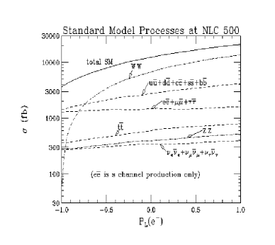
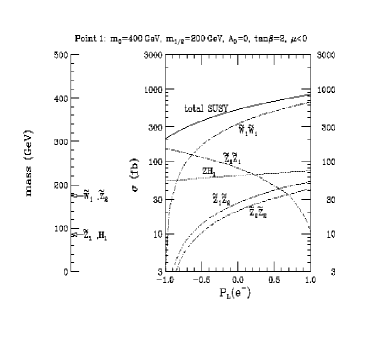
Figure 2: Cross sections of different SM processes as well as the chargino/neutralino production. The values of the model parameters are mentioned in the figure.

cross-sections for different SM processes and the corresponding ones for the SUSY model dependent chargino/neutralino pair production, at a chosen point in the mSUGRA parameter space. From the figure it is clear that with a judicious choice of polarization of $e^{-}$/$e^{+}$ beam, the SM background can be handled and precision measurements of chargino/neutralino sector are possible. The $e^{+}e^{-}$ collider produces democratically all the sparticles that have EW couplings. Hence it is better suited than the LHC to study the gauginos/higgsinos and sleptons and will complement the information in these sectors from the LHC very effectively. The correlation between properties of gluino that will be obtained from the LHC and those of chargino/neutralino sector from LHC/LC can disentangle the various gaugino mass parameters $M_{i}$ at weak scale. For reasons outlined in the introduction knowledge about the relative values of $M_{i}(i=1,3)$ at the weak scale, from independent sources, contains crucial clues to the physics at high scale. This also shows how truly the LHC and LC are complementary to each other and thus how necessary both are to solve the puzzle of EWSB.

What and How well can LC measure

There have been a large number of dedicated studies tata2 ; MP1 ; extra3 ; ACC ; extra4 ; extra5 ; teslatdr ; zerwastlk ; extra6 of the possibilities of precision measurements of the sleptons extra6 ; FM1 ; MIHO1 ; tata2 ; MIHO2 ; MB1 ; SM , squarks FF ; tata2 ; SM ; DEKG ; stop_mc , charginos/neutralinos extra6 ; tata2 ; FM1 ; FS ; MB1 ; Z1 ; Z2 ; Z3 ; extra7 ; MGP1 ; kneur1 ; kneur and Higgses MB . Study of third generation sfermions MIHO1 ; MIHO2 ; SM are shown to yield particularly interesting information about SUSY models. Almost no study is possible without use of polarisation, at least for one of the initial state fermions. A detailed discussion of the special advantages, in general, of using polarisation of both the beams is available elsewhere in the proceedings gtalk . In this talk I do not include discussion of the SUSY Higgses as it is also discussed somewhere else in the proceedings MB and also because the dependence of the Higgs sector on SUSY breaking parameters and hence on the high scale physics is essentially only through the loop corrections.

Precision measurements of masses

Sleptons and Charginos/Neutralinos

The masses of sleptons can be determined at an LC essentially using kinematics. Making use of partial information from the LHC, it will be possible to tune the energy of the LC to produce the sfermions sequentially. The pair produced lightest sleptons will decay through a two body decay. Let us take the example of $\widetilde{\mu}_{R}$ which will have the simplest decay. So one has in this case,

$$e^{+}e^{-}\to\tilde{\mu}_{R}\tilde{\mu}_{R}^{*}\to\mu^{+}\mu^{-}\tilde{\chi}_{1}^{0}\tilde{\chi}_{1}^{0}$$ (1)

Since the slepton is a scalar the decay energy distribution for the $\mu$ produced in two body decay of $\widetilde{\mu}_{R}$, will be flat with

$${m_{\widetilde{\mu}_{R}}\over 2}\left(1-{{m_{\widetilde{\chi}^{0}_{1}}^{2}}\over{m_{\widetilde{\mu}_{R}}^{2}}}\right)\gamma(1-\beta)<E_{\mu}<{m_{\widetilde{\mu}_{R}}\over 2}\left(1-{{m_{\widetilde{\chi}^{0}_{1}}^{2}}\over{m_{\widetilde{\mu}_{R}}^{2}}}\right)\gamma(1+\beta).$$ (2)

Thus measuring the end points of the $E_{\mu}$ spectrum accurately will yield a precision measurement of the masses $m_{\widetilde{\mu}_{R}}$, $m_{\widetilde{\chi}^{0}_{1}}$. Of course, one has to contend with the background from $W^{+}W^{-}$ and the $\widetilde{\chi}^{0}_{1}\widetilde{\chi}^{0}_{2}$ production (cf. Fig. 2). As can be seen from the right panel of the same figure, this can be handled by choosing polarised $e^{-}/e^{+}$ beams. Fig. 3 taken from Ref. MB1 shows that

Figure 3: Precision of mass determination for $\widetilde{\mu}_{L}$ and $\widetilde{\mu}_{R}$ at TESLA with $500~{}{\rm fb}^{-1}$, with $P_{e^{-}}/P_{e^{+}}=0.8/0.6$, taken from the studies in MB1 . Details of the values of the mSUGRA parameters are given there.

$\tilde{\mu}_{R}$ mass can be determined to a precision of 0.3 % at TESLA with $\int{\cal L}dt$ = 500 f$b^{-1}$. The analysis uses both $e^{-}$/$e^{+}$ beam polarisations, with $P_{e^{-}}/P_{e^{+}}=80\%/60\%$. The need for polarisation of both the beams is discussed elsewhere in the proceedings gtalk . The panel on right shows, for the same point in mSUGRA parameter space as the panel in left, signal for production of $\widetilde{\mu}_{L}^{*}\widetilde{\mu}_{L}$ and its three body decay via

$$e^{+}e^{-}\to\widetilde{\mu}_{L}\widetilde{\mu}_{L}^{*}\to\mu^{-}\widetilde{\chi}^{0}_{2}\mu^{+}\widetilde{\chi}^{0}_{2}\to\mu^{-}\mu^{+}\widetilde{\chi}^{0}_{1}\widetilde{\chi}^{0}_{1}l^{+}l^{-}{l^{\prime}}^{+}{l^{\prime}}^{-}$$ (3)

For the particular point in the mSUGRA parameter space they have chosen, the branching ratio for $\widetilde{\mu}_{L}\to\mu\widetilde{\chi}^{0}_{2}$ is substantial and the cleanliness of the final state compensates for the eventual small rates. Thus $\widetilde{\mu}_{L}$ mass determination to percent level seems possible for TESLA MB1 . However, the method of using the end point of the energy spectrum will not work so well, e.g. , for $\widetilde{\tau}_{1}\widetilde{\tau}_{1}^{*}$ production and decay.

Another method for precision determination of the masses of the sleptons and the lighter charginos/neutralinos, is to perform threshold scan. The linear $\beta$ dependence as opposed to the $\beta^{3}$ dependence of the cross-section, near the threshold (where $\beta$ is the c.m. velocity of the produced sparticle) makes the method more effective for the spin 1/2 charginos/neutralinos than the sleptons. Of course, such threshold scans will require very high luminosity. The efficacy of the method of threshold scans has been studied in the context of the high luminosity TESLA collider  MB1 . The results of their study for a chosen point in the mSUGRA parameter space are summarized in Table  2.

Table 2: Kinematic mass determinations at TESLA for threshold scans with $10$ fb ^-1 luminosity per energy, for the mSUGRA point RR1 of the TESLA studies teslatdr .

particle	m	$\delta m_{cont}$	$\delta m_{scan}$	Can give info.on
$\widetilde{\mu}_{R}$	132.0	0.3	0.09	$m_{0}$, $m_{1/2}$, $\tan\beta$
$\widetilde{\mu}_{L}$	176.0	0.3	0.4
$\widetilde{\nu}_{\mu}$	160.6	0.2	0.8
$\widetilde{e}_{R}$	132.0	0.2	0.05
$\widetilde{e}_{L}$	176.0	0.2	0.18
$\widetilde{\nu}_{e}$	160.6	0.1	0.07
$\widetilde{\tau}_{1}$	131.0		0.6	$m_{0}$, $m_{1/2}$,$\mu$, $\tan\beta$
$\widetilde{\nu}_{\tau}$	160.6		0.6
$\widetilde{\chi}^{\pm}_{1}$	127.7	0.2	0.04	$M_{2}$, $\mu$, $\tan\beta$
$\widetilde{\chi}^{\pm}_{2}$	345.8		0.25
$\widetilde{\chi}^{0}_{1}$	71.9	0.1	0.05	$M_{1}$,$M_{2}$, $\mu$, $\tan\beta$
$\widetilde{\chi}^{0}_{2}$	130.3	0.3	0.07
$\widetilde{\chi}^{0}_{3}$	319.8		0.30
$\widetilde{\chi}^{0}_{4}$	348.2		0.52

This requires about $100~{}{\rm fb}^{-1}$ luminosity distributed over 10 energy values for each sparticle. For the $\widetilde{\nu}_{e}$ the high accuracy of the mass determination is possible because of the large cross-section due to the $t$ channel contribution. For the $\widetilde{\nu}_{\mu}$ and $\widetilde{\nu}_{\tau}$, however the rates are smaller by more than an order of magnitude for the point chosen for the study. Recent analyses of the mass determination of $\widetilde{\tau}_{1}$  and ${\widetilde{\nu}}_{\tau_{1}}$ tata3 using the continuum production, show that with the latter method only an accuracy of $\sim 2\%$ for $m_{\widetilde{\tau}_{1}}$ (consistent with the earlier analyses MIHO2 ) and even much worse $6-10\%$ for $m_{\widetilde{\nu}_{\tau}}$, is possible even after a use of optimal polarisation and comparable luninosities as in the threshold scan case. This shows that the threshold scan method will offer a better measurement in general. The very high efficiency for $\tau$ detection in the TESLA environment might also be playing a role in this difference in the accuracies as the other analyses MIHO1 ; MIHO2 ; tata3 use the full Monte Carlo simulation using the hadronic decay products of the $\tau$. However, that does not seem to be the full story. While it is true that the threshold scan methods will possibly yield more accurate measurement of masses as compared to the continuum, the low rates for the $\widetilde{\nu}_{\tau},\widetilde{\tau}_{2}$ might force one to go away from the threshold somewhat, thus sacrificing the accuracy. Note also that the branching ratios of the $\widetilde{\nu}_{\tau}$ into different channels are not going to be known, a priori. This means that the normalisation, along with shape will also have to be fitted to the observed event rate, which measures cross-section (which we want to measure to determine mass) times the branching ratio. While it is not clear how much this will affect the precision with which mass can be extracted, it will certainly lead to some degradation of its measurement. A preliminary study underway tata4 to address these issues does not seem to reproduce the high accuracy of the mass measurements for $\widetilde{\nu}_{\tau},\widetilde{\nu}_{\mu}$, even for the threshold scan. It is very important to clearly understand just how well these measurements can be made, as these accuracies affect, crucially, the projected abilities to gleen information about the SUSY breaking scale.

Using $e^{-}e^{-}$ collisions instead of $e^{+}e^{-}$ gives an interesting advantage in the study of selectron production fee . $\widetilde{e}_{R}\widetilde{e}_{R}$ production in $e^{-}e^{-}$ collisions proceeds only through the $t$ channel diagram as opposed to the case of $e^{+}e^{-}\to\widetilde{e}^{*}_{R}\widetilde{e}_{R}$ production and hence has a threshold rise $\propto\beta$ instead of the $\beta^{3}$ as in the latter case. The former makes the study of $\widetilde{e}_{R}$ production in $e^{-}e^{-}$ collisions much more sensitive to the nature of $\widetilde{\chi}^{0}_{1}$ and the latter has the potential of increasing the accuracy of the $\widetilde{e}_{R}$ mass determination through threshold scans. This difference in the threshold rise of the cross-sections in the two cases is shown in Fig. 4 taken from fee .

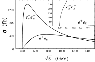
Figure 4: Different threshold rise of $\widetilde{e}_{R}\widetilde{e}_{R}^{*}$ and $\widetilde{e}_{R}\widetilde{e}_{R}$ production cross sections for $e^{+}e^{-}$ and $e^{-}e^{-}$ processes respectively, taken from fee .

However, it must be pointed out that this study does not include effects of beamstrahlung and ISR. A report presented at this meeting heusch shows that these might blur the distinction, at least for the X-band designs. Also it should be remembered that selectrons are the only sparticles that can be produced at an $e^{-}e^{-}$ collider.

The subpermille achievable accuracy for sparticle mass measurements that the analysis in Ref. MB1 (cf. Table 2) seems to indicate by the threshold scan method, underlies the need of the study of higher order effects in all the studies and that has become the state of the art of theoretical calculations. Inclusion of effects of the finite width of the smuon MB2 or that of higher order corrections to $\widetilde{\chi}^{+}_{i}\widetilde{\chi}^{-}_{j}$ production extra9 or the contribution of the nonresonant production of $\mu^{+}\mu^{-}\widetilde{\chi}^{0}_{1}\widetilde{\chi}^{0}_{1}$  freitas on the precision of the mass measurement using threshold scans are being studied.

Squarks

Clearly squarks are the only strongly interacting particles about whom direct information can be obtained at the $e^{+}e^{-}$ collider. For the strongly interacting sfermions (squarks) the decay is $\widetilde{q}\to q\widetilde{\chi}^{0}_{1}$. As a result, one has to study the end point of the distribution in $E_{jet}$. The hadronization effects can in principle deteriorate the accuracy of the determination of $m_{\widetilde{q}}$. An alternate estimator  FF of $m_{\tilde{q}}$ is the peak of the distribution in the minimum kinematically allowed mass of the $q\widetilde{\chi}^{0}_{1}$ system produced in

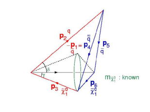
Figure 5: Determination of the minimum kinematically allowed squark mass, following Ref. FF .

$\tilde{q}$ decay; $m_{\tilde{q},min}$. The minimum squark mass corresponds to maximum possible $|\vec{p}_{4}|$ and can be easily determined following the construction in Fig. 5. The figure in the left panel of Fig. 6, taken from Ref. FF shows the efficacy of this estimator for a 500 GeV machine with $10$ fb^-1 luminosity per polarisation, the latter

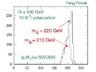
Figure 6: Accuracy of determination of $m_{\widetilde{q}}$ using the $m_{\widetilde{q},min}$ defined in FF .

being used for separating $\widetilde{q}_{L}/\widetilde{q}_{R}$ contributions, for a particular point in the MSSM parameter space. Figure in the right panel shows that this variable provides a good estimate of $m_{\widetilde{q}}$ even after radiative corrections, both in production and decay, have been included DEKG .

If the squarks are lighter than the glunios, any information on gluino masses at an $e^{+}e^{-}$ collider can only come from the assumed relations between the masses of the electroweak and strong gauginos.

Precision determination of mixings

The mixing between various interaction eigenstates in the gaugino sector as well as the, in general, large mixing in the L-R sector for the third generation squarks and sleptons, is decided respectively by $M_{1},M_{2},\mu,\tan\beta$ and $\mu,\tan\beta,A$ as well as various scalar mass parameters. So clearly an accurate measurement of these mixings along with the precision measurements of masses offers further clues to physics at high scale. Table 2 shows in the last column the parameters whose values can be extracted from mass measurements of various EW sparticles; the sleptons and the chargino/neutralinos.

Possibilities of the determination of L-R mixing in the third generation sfermions have been investigated MIHO1 ; MIHO2 ; SM . The mass eigenstates can be written down in terms of the interaction eigenstates for, e.g. , staus as $\widetilde{\tau}_{1}=\widetilde{\tau}_{L}\cos\theta_{\tau}+\widetilde{\tau}_{R}\sin\theta_{\tau}$,$\widetilde{\tau}_{2}=\widetilde{\tau}_{L}\sin\theta_{\tau}+\widetilde{\tau}_{R}\cos\theta_{\tau}$. It is clear that polarised $e^{-}$/$e^{+}$ beams can play a crucial role in determining $\theta_{\tau}$. Let us, for example, consider $e^{+}e^{-}\to\widetilde{\tau}_{1}\widetilde{\tau}_{1}^{*}$. Further let us consider the case of 100 % polarisation in particular. The pair production proceeds through an exchange of $\gamma$/Z in $s$-channel. For energies $\sqrt{s}$ $>$ $>$ $m_{Z}$, with $P_{e^{-}}$ = 1, one can essentially interpret this $s$-channel exchange of $\gamma$/Z as an U(1) gauge boson, $B$. In this limit $\sigma(\widetilde{\tau}_{R})$ = 4 $\sigma(\widetilde{\tau}_{L})$. Thus it is clear that a measurement of $\sigma(e^{+}e^{-}\to\widetilde{\tau}_{1}^{*}\widetilde{\tau}_{1})$ along with a knowledge of polarisation of $e^{-}$ beam can lead to an extraction of $\cos\theta_{\tau}$. Further the polarisation of $\tau$ produced in $\widetilde{\tau}_{1}$ decay provides a measurement of the mixing angle in the neutralino sector as well. Let us consider $\widetilde{\tau}_{R}\to\tau\widetilde{\chi}^{0}_{1}$ depicted in Fig. 7. The $\tilde{B}$ component of $\widetilde{\chi}^{0}_{1}$ produces $\widetilde{\tau}_{R}$, whereas the higgsino

Figure 7: $\widetilde{\tau}_{R}\to\tau\widetilde{\chi}^{0}_{1}$.

component will flip the chirality and produce $\widetilde{\tau}_{L}$. Thus the measurement of $\widetilde{\tau}_{1}^{*}\widetilde{\tau}_{1}$ production with polarised $e^{-}$ beams and the polarisation of decay $\tau^{s}$ can give very useful information on both the mixings: the $L-R$ mixing in the stau sector and the mixing in the neutralino sector. The $\tau$ polarisation can be measured by looking at the energy distribution of the decay product $\rho$ in the hadronic decay of $\tau$ MIHO1 .

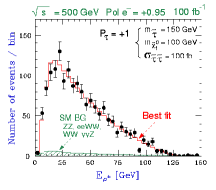
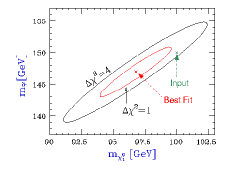
Figure 8: Precision of the determination of $m_{\widetilde{\tau}_{1}}$ and $m_{\widetilde{\chi}^{0}_{1}}$ for luminosities and polarisation mentioned in the figure. Taken from Ref.MIHO2 .

Fig. 8 MIHO2 shows the possible accuracy of a simultaneous determination of $m_{\tilde{\tau_{1}}}$ - $m_{\tilde{\chi_{1}^{0}}}$ from the determination of the end points of the energy spectrum, for $\int{\cal L}dt=100\ {\rm fb}^{-1},P_{e^{-}}=0.95$ and $\sqrt{s}=500$ GeV. The input value lies outside the $\Delta\chi^{2}$ = 1 contour around the best fit value. However, if $m_{\widetilde{\chi}^{0}_{1}}$ is assumed to be known, then $\Delta m_{\widetilde{\tau}_{1}}$ goes down considerably and a 1-2% determination at

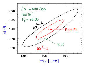
Figure 9: Simultaneous determination of $\sin\theta_{\tau}$ and $m_{\widetilde{\tau}_{1}}$, taken from Ref.MIHO2 .

$1\sigma$ level is possible. Fig. 9 shows accuracy of sin$\theta_{\tau}$ determination for the same choice of parameters and we see that $\Delta(\sin\theta_{\tau})<0.03$.

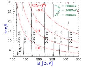
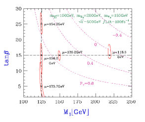
Figure 10: Contours of constant cross-section in $M_{1}$ - tan$\beta$ plane and accuracy of tan$\beta$ measurement, taken from Ref. MIHO2 .

Further, Fig. 10 MIHO2 shows in the left panel the contours of constant cross-section $\sigma(e^{+}e^{-}\to\widetilde{e}_{R}^{*}\widetilde{e}_{R})$, and of constant polarisation $P_{\tau}$ ( $\widetilde{\tau}_{R}\to\tau\tilde{\widetilde{\chi}^{0}_{1}}$) in the $M_{1}$ - $\tan\beta$ plane (this analysis assumes universal gaugino masses at a high scale). The figure in the right panel shows the accuracy one can expect from a simultaneous study of these two measurements. It shows that the method has potential of a good $\tan\beta$ determination at large $\tan\beta$.

Left panel in Fig. 11 SM ; teslatdr shows contours of constant cross-section for

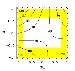
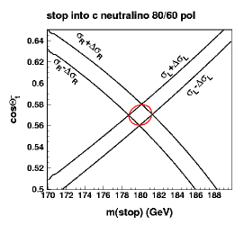
Figure 11: Polarisation dependence of the production cross-section for $\widetilde{t}_{1}\widetilde{t}_{1}^{*}$ pair and the expected accuracy of a simultaneous determination of $\cos\theta_{t}$ and $m_{\widetilde{t}_{1}}$ at the TESLA collider.

$\widetilde{t}_{1}\widetilde{t}_{1}^{*}$ production at TESLA for $m_{\widetilde{t}_{1}}=180$ GeV and $\cos\theta_{t}=0.57$ as a function of the polarisation $P_{-}$/$P_{+}$ of the $e^{-}$/$e^{+}$ beam. This shows how it is important to have polarisation for both beams. The right panel stop_mc ; teslatdr shows also the accuracy of $\cos\theta_{t}$ - $m_{\widetilde{t}}$ measurement using $\widetilde{t}_{1}\to c\widetilde{\chi}^{0}_{1}$ decay mode for stops and 80/60 polarisation for $e^{-}$/$e^{+}$ beam. The figure shows that at TESLA one can reach $\Delta(\cos\theta_{t})=0.003,\Delta(m_{\widetilde{t}})=0.08$. It is interesting to note that if $m_{\widetilde{t}_{1}}$ is in the mass range of 180-225 GeV , the $2\gamma$ decay mode of the lightest higgs may not be accessible at the LHC and even the visibility of the $\widetilde{t}_{1}$ in this mass range at the LHC has not been completely analysed.

A study of the chargino sector at the LC can provide a precision determination of the higgsino-gaugino mixing and consequently an accurate determination of all the Lagrangian parameters which dictate the properties of the chargino sector. This requires, along with the determination of $m_{\widetilde{\chi}^{\pm}_{1}},m_{\widetilde{\chi}^{0}_{1}}$ and $\sigma^{\rm tot}_{\widetilde{\chi}^{+}_{1},\widetilde{\chi}^{-}_{1}}$, a study of either the dependence of the production cross-section on the initial beam polarisations or the polarisation of the produced charginos through the angular distribution of their decay products. Since $\sigma(e^{+}e^{-}\to\widetilde{\chi}^{-}_{i}\widetilde{\chi}^{+}_{j})$ depends on $m_{\widetilde{\nu}}$, its knowledge is also necessary. This can be obtained by studying the energy dependence of the $\sigma^{\rm tot}$, even if $m_{\widetilde{\nu}}$ is beyond the kinematic range of the collider. If only the lightest chargino is available kinematically, then one can determine the mixing angles in the chargino sector $\Phi_{L},\Phi_{R}$ defined through

$$\widetilde{\chi}^{-}_{1L}=\cos\Phi_{L}\tilde{W}^{-}_{L}+\sin\Phi_{L}\tilde{H}^{-}_{2L},\widetilde{\chi}^{-}_{1R}=\cos\Phi_{R}\tilde{W}^{-}_{R}+\sin\Phi_{R}\tilde{H}^{-}_{1R},$$ (4)

only upto a two fold ambiguity. However, this can be removed, using the information on the transverse polarisation, as shown in Fig. 12. If both the charginos are accessible kinematically, $\cos 2\Phi_{R},\cos 2\Phi_{L}$ can be determined uniquely through measurements of $\sigma_{L/R}(\widetilde{\chi}^{+}_{i}\widetilde{\chi}^{-}_{j})$, as shown in the lower panel

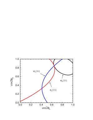
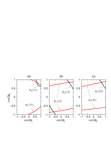
Figure 12: Demonstration of unique determination of mixing angles in the chargino sector using polarised beams Z1 ; Z2 ; Z3 .

of the same figure. It has been shown, in a purely theoretical study  Z1 ; Z2 , in the context of TESLA, using only statistical errors, that with $\int{\cal L}dt=1\ ab^{-1},\cos 2\Phi_{L},\cos 2\Phi_{R}$ can be determined to an accuracy of $\sim 1-3\%$. Along with the information on $m_{\widetilde{\chi}^{+}_{i}}$ the mixing angles can then lead to an unambiguious determination of the Lagrangian parameters $M_{2},\mu$ and $\tan\beta$. However, since all the variables are proportional only to $\cos 2\beta$, the accuracy of $\tan\beta$ determination is rather poor at high $\tan\beta$. At high $\tan\beta$, measurements in the slepton sector (stau/selectron) discussed earlier MIHO2 afford a better determination. Alternative ways of extracting $\tan\beta$ from a study of the Higgs sector  feng_h ; han have been suggested. But of course these need access to the heavier higgses $A,H$ and $H^{\pm}$. In view of the current LEP limits on the $\tan\beta-m_{A}$ plane, indications are that such determination might require $\sqrt{s}$ values larger than the $500$ GeV that is envisaged in the first stage for an LC. A better handle on the $\tan\beta$ in the large $\tan\beta$ range is offered by the studies of the $H/A,H^{\pm}$ sector at the LHC atlas_tdr .

Similar studies of the neutralino sector MGP1 ; kneur1 ; kneur show that one can extract $\tan\beta,M_{2},\mu$ as well as the relative phase of $\mu/M_{2}$ kneur in case it is nonzero. Use of polarisation for both the beams gtalk allows extraction of $M_{1},M_{2},\mu$ and $\tan\beta$, without assuming the unification relation among $M_{1},M_{2}$ MGP1 . Availability of polarisation of both the beams seems to increase the accuracy of the measurement substantially. The sensitivity to the departure from the universal gaugino masses increases further wuerz by using the $e\gamma$ option of the collider should that be realised.

Scenarios other than mSUGRA and MSSM

AMSB

Another interesting set of studies of the chargino/slepton sector is in the context of the AMSB models, wherein one expects an almost degenerate pair of the lightest neutralino/chargino which are essentially winos. Since the mass difference is expected to be $165~{}{\rm MeV}<\Delta M<1$ GeV, $\widetilde{\chi}^{+}_{1}$ has $\sim 96\%$ B.R. in the $\pi^{+}\widetilde{\chi}^{0}_{1}$ channel. Depending on the mass-difference $m_{\widetilde{\chi}^{+}_{1}}-m_{\widetilde{\chi}^{0}_{1}}$ and hence the life time of $\widetilde{\chi}^{+}_{1}$, the signature can be either a high momentum track stoping in the vertex detector or a displaced vertex which can be inferred from the impact parameter of the soft decay pion. Feasibility of studying the pair production of the charginos  gm as well as the left selectrons(smuons) dsp , at the NLC in this scenario has been demonstrated. The study gm shows that using different techniques, it is possible to probe the chargino/neutralino masses right upto the kinematic limit even in this case.

Unstable $\widetilde{\chi}^{0}_{1}$

As discussed in the introduction, the $\widetilde{\chi}^{0}_{1}$ is not necessarily stable if $R$ parity is broken or gravitino is the LSP. In the case of $R_{p}/\;\>$ apart from the very clean and striking signals due to production of single sparticle resonance through the $R_{p}/\;\>$ couplings there have also been beginnings of detailed investigations grr of possibility of studying the sparticle signals at the LC in this scenario, when the $R_{p}/\;\>$ couplings are small and hence the effect of $R_{p}/\;\>$ is seen only in the decay of the $\widetilde{\chi}^{0}_{1}$. Indeed, the decays of the lightest neutralino give rise to significant and striking signals which can be studied with ease at an LC, for the case of lepton number violating $\lambda$ and $\lambda^{\prime}$ couplings. Interestingly, even in the case of the $B/\;\>$ $\lambda^{\prime\prime}$ couplings, it seems possible, not only to see the signal due to the gaugino/higgsino production, but also to get information on the mass of the lightest neutralino in this case, which would be particularly difficult for the hadronic colliders to measure.

In the case of GMSB models, the difference in the search strategy of the sparticles indeed comes only from the decay of the $\widetilde{\chi}^{0}_{1}$ (or for that matter that of the NLSP). In the literature invesitgations exist for the case where $\widetilde{\chi}^{0}_{1}$ is the NLSP AB as well as when $\widetilde{\tau}_{1}$ is the NLSP HH . The former study includes very detailed analysis of the signals for a decaying $\widetilde{\chi}^{0}_{1}$, for a wide range of GMSB models. The dominant decay of the neutralino NLSP is always into a $\tilde{G}\gamma$ channel. If the lifetime of the NLSP is large, pair production of $\widetilde{\chi}^{0}_{1}$ and their decay, can give rise to one or more nonpointing photons, due to the delayed decay of the NLSP. For larger masses of the NLSP $(\geq 100$ GeV) two body decay into a $Z_{0}\gamma$ channel followed by the $Z_{0}$ decay into a $f\bar{f}$ pair, can provide a cleaner signature. A measurement of the upper end point of the energy spectrum of the decay photon from the $\tilde{G}\gamma$ decay, can provide an accurate measurement of the mass of $\widetilde{\chi}^{0}_{1}$. For example, with an integrated luminosity of $200\;{\rm fb}^{-1}$, for a $\widetilde{\chi}^{0}_{1}$ mass $200$ GeV, a measurement of $\sim 0.2\%$ accuracy is possible. This is demonstrated in Fig. 13. We will see later, how this can prove very useful in determining the SUSY breaking scale in this case.

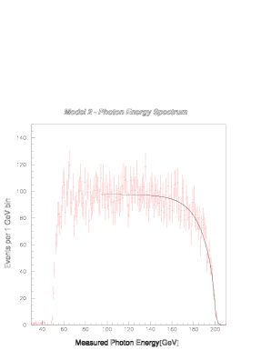
Figure 13: Accuracy of mass of $\widetilde{\chi}^{0}_{1}$ at an LC for GMSB models which have the $\widetilde{\chi}^{0}_{1}$ as the NLSP, taken from Ref.AB .

Determination of quantum numbers of the sparticles

Above discussion already shows how an efficient use of polarisation of both $e^{+}/e^{-}$ beams, allows a high precision determination of the mixings among the $L-R$ sfermions as well as in the gaugino-higgsino sector. This is, indeed, indirectly a determination of the hypercharges of the various sparticles. It has been demonstrated  FM1 , using realistic simulation of the backgrounds, that it is possible to reconstruct the $\widetilde{\mu}$ angular distribution in the process $e^{+}e^{-}\to\widetilde{\mu}\widetilde{\mu}^{*}\to\mu^{+}\mu^{-}+E_{T}/\;\>$   and hence determine the spin of the smuon with precision. Further, the cross-section of $\widetilde{e}_{R}\widetilde{e}_{R}^{*}$ production can be used as a very sensitive probe of the equality of the couplings $g_{\widetilde{e}e_{R}\tilde{B}}$ and $g_{eeB}$. This is due the contribution of the $t$ channel diagram shown in the left-hand panel of Fig. 14, which involves a $\widetilde{\chi}^{0}_{i}$ exchange. The contribution

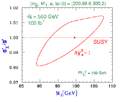
Figure 14: Simultaneous determination of $M_{1}$ and $g_{\widetilde{e}_{R}e\widetilde{B}}$, in a study of $\widetilde{e}_{R}\widetilde{e}_{R}^{*}$ production.

to the production cross-section of the $\widetilde{e}_{R}\widetilde{e}_{R}^{*}$ pair is sensitive to the bino component of $\widetilde{\chi}^{0}_{i}$ and hence to the $U(1)$ gaugino mass parameter $M_{1}$ and the coupling $g_{\widetilde{e}_{R}e_{R}B}$. At tree level we expect, due to supersymmetry,

$$g_{\widetilde{e}_{R}e_{R}\tilde{B}}=g_{eeB}=\sqrt{2}g_{2}\tan\theta_{W}=\sqrt{2}g_{1}Y_{b}=g_{Y}.$$ (5)

Using $\sigma(e^{+}e^{-}\to\widetilde{e}_{R}\widetilde{e}_{R}^{*})$ and $\frac{d\sigma}{d\cos\theta}(e^{+}e^{-}\to\widetilde{e}_{R}\widetilde{e}_{R}^{*})$, one can determine $g_{\widetilde{e}_{R}e_{R}\tilde{B}}$ and $M_{1}$ simultaneously. For an integrated luminosity of $100\ {\rm fb}^{-1}$, $Y_{b}$ of Eq. 5 can be determined to an accuracy of $1\%$ MIHO2 . This is shown in the right panel of Fig. 14. This expected accuracy is actually comparable to the size of the SUSY radiative corrections MIHO3 to the tree level equality of Eq. 5 and hence this measurement can serve as an indirect probe of the mass of the heavy sparticles. We will get to this later.

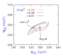
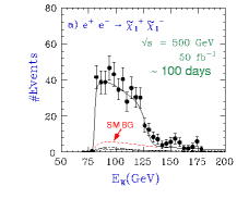
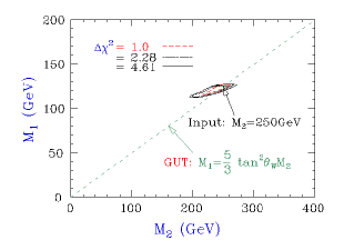
Figure 15: Simultaneous determination of chargino/neutralino mass from chargino studies and consequent testing of the GUT relation between $M_{1}$ and $M_{2}$ FM1 .

Accurate high statistics measurements of the chargino system, provided both the charginos are accessible, also afford a good test of the equaility of $g_{e\nu W}$ and $g_{e\widetilde{\nu}\tilde{W}}$. For the representative points in the SUGRA parameter space, chosen for the TESLA studies Z3 , the relation can be tested to $0.1\%$ for an integrated luminosity of $1~{}{\rm ab}^{-1}$. It should be noted however, that this study uses only the statistical errors in the analysis. The above discussion thus shows that at an LC one can indeed measure the equality of the couplings which is the cleanest evidence for supersymmetry.

Determination of the SUSY breaking parameters at high scale and the SUSY breaking scale

The precision measurements of the masses and the mixings in the sfermion and the chargino/neutralino sector at the LC will certainly allow to establish existence of supersymmetry as a dynamical symmetry of particle interactions. However, this is not all these measurements can achieve. The high precision of these measurements will then allow us to infer about the SUSY breaking scale and the values of the SUSY breaking parameters at this high scale, just the same way the high precision measurements of the couplings $g_{1},g_{2}$ and $g_{3}$ can be used to get a glimpse of the physics of unification and its scale, as has been shown in Fig. 1.

There are essentially two different approaches to these studies. In the pioneering studies  FM1 ; MIHO2 , the JLC group investigated how accurately one can determine the parameters $M_{1},M_{2},\mu,\tan\beta$ and $m_{0}$ at the high scale by fitting these directly to the various experimental observables such as the polarisation dependent production cross-sections of the sparticles, angular distributions of the decay products etc., that have been mentioned in the discussion so far. An example of this is shown in Fig. 15. The right hand figure in the top panel shows how a determination of the energy distribution of the ‘W’ produced in the decay of $\widetilde{\chi}^{+}/\widetilde{\chi}^{-}$, in the reaction $e^{+}e^{-}\to\widetilde{\chi}^{+}_{1}\widetilde{\chi}^{-}_{1}$, affords a determination of $m_{\widetilde{\chi}^{0}_{1}}$ and $m_{\widetilde{\chi}^{\pm}}$ shown in the left panel. The lower panel then shows how using the masses $m_{\widetilde{\chi}^{\pm}},m_{\widetilde{\chi}^{0}_{1}}$ along with $\sigma_{R}(\widetilde{\chi}^{\mp}_{1}),\sigma_{R}(\tilde{e}_{R})$ and the angular distribution of the decay leptons one can extract $M_{1},M_{2}$ at the GUT scale and test the GUT relation.

A different approach zerwastlk ; MB1 ; extra7 ; kneur1 is to use the experimental observables such as cross-sections, angular distributions to determine the physical parameters of the system such as masses and mixings and then use these to determine the Lagrangian parameters $M_{1},M_{2},\mu,\tan\beta$ at the EW scale itself. Thus the possible errors of measurements of the experimental quantities alone will control the accuracy of the detrmination of these parameters. There are again two ways in which this information can be used: one is a top down approach which in spirit is similar to the earlier one as now one uses these accurately determined Lagrangian parameters at the EW scale to fit their values at the high scale and then compare them with the input value. It has been shown MB1 in this approach, that the projected accurate measurements of the various sparticle masses through threshhold scans with a very high luminosity run of TESLA (one will require a threshold scan using ten points with $10$ ${\rm fb}^{-1}$ at each point, for each sparticle and appropriately higher energies for the heavier ones), allows a determination of the values of $M_{1},M_{2},m_{0},\mu$ and $\tan\beta$ at the high scale to an accuracy of better than $1\%$. As mentioned earlier the accuracy is much worse for higher values of $\tan\beta$. The expected accuracy of determination of the trilinear term is rather poor as shown in Tables 4 and 4 taken from Ref. MB1 . This deterioration is due to the fact that most of the physical observables are rather insensitive to the parameters $A_{k}$.

Table 3: Reconstruction of SUGRA parameters assuming universal masses.

	True value	Error
$m_{0}$	100	0.09
$m_{1/2}$	200	0.10
$A_{0}$	0	6.3
tan$\beta$	3	0.02

Table 4: Reconstruction of SUGRA parameters with nonuniversal guagino masses.

	True value	Error
$m_{0}$	100	0.09
$M_{1}$	200	0.20
$M_{2}$	200	0.20
$A_{0}$	0	10.3
tan$\beta$	3	0.04

A completely different and a very interesting way of using the information on these masses PZB is the bottom up approach where, one starts with these Lagrangian parameters extracted at the weak scale and use the renormalisation group evolution (RGE) to calculate these parameters at the high scale. As explained in the introduction, different SUSY breaking mechanisms differ in their predictions for relations among these various parameters at the high scale. The ineteresting aspect of the bottom up approach is the possibility they offer of testing these relations ‘directly’ by reconstructing them from their low energy values using the RGE. In the analysis the ‘experimental’ values of the various sparticle masses are generated in a given scenario (mSUGRA,GMSB etc.) starting from the universal parameters at the high scale appropriate for the model under consideration and using the evolution from the high scale to the EW scale. These quantities are then endowed with experimental errors expected to be reached in the combined analyses from LHC and an LC with energy upto $1$ TeV , with an integrated luminosity of $1{\rm ab}^{-1}$. Then these values are evloved once again to the high scale. The figure in the left panel of Fig. 16

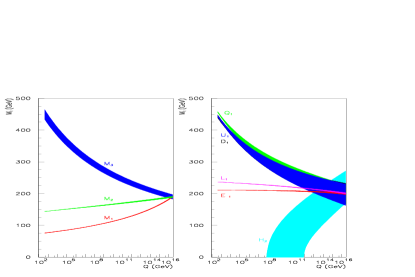
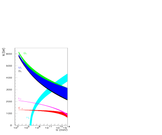
Figure 16: Bottom up approach of the determination of the sparticle mass parameters for mSUGRA and GMSBPZB . Values of the model parameters as given there.

shows results of such an exercise for the gaugino and sfermion masses for the mSUGRA case and the one on the right for sfermion masses in GMSB. The width of the bands indicates $95\%$ C.L. Bear in mind that such accuracies will require a 10-20 year program at an LC with $\sqrt{s}\leq 1.5$ TeV.

The two figures in the left panel show that with the projected accuracies of measurements, the unification of the gaugino masses will be indeed demonstrated very clearly. The errors in the evolution of the slepton masses are rather small as only the EW gauge couplings contribute to it. This is seen in the second figure in left panel of the figure, which shows the evolved squark, slepton and the Higgs masses. The unification of the slepton masses at the high scale can be demonstrated quite precisely. The errors on the reconstruction of the universal mass from squark and higgs masses, are rather large. In the case of the Higgs mass parameters this insenstivity to the common scalar mass $m_{0}$ is due to an accidental cancellation between different contributions in the loop corrections to these masses which in turn control the RG evolution. In the case of squarks the errors in the extrapolated values are caused by the stronger dependence of the radiative corrections on the common gaugino mass, due to the strong interactions of the squarks. As a result of these a small error in the latter can magnify in the solution of $m_{0}$. Further, the trilinear $A$ coupling for the top shows a pseudo fixed point behaviour, which again makes the EW scale value insensitive to $m_{0}$. If the universal gaugino mass $m_{1/2}$ is larger than the $m_{0}$ then this pesduo fixed point behaviour increases the errors in the determination of third generation squark mass at the EW scale. This picture shows us clearly the extent to which the unification at high scale can be tested. If we compare this with the results of Tables 4 and 4, we see that with the bottom up approach we have a much clearer representation of the situation. The $95\%$ C.L. bands on the squark and the higgs mass parameters get much wider if one assumes only the accuracies expected to be reached at the LHC collider BWS . Thus we see that an LC can help crucially in trying to give a clearer picture of the SUSY breaking parameters at the high scale.

The figure in the right panel shows the results of a similar exercise but for GMSB model, where with the assumed values of the model parameters, one would need to have a $1.5$ TeV LC to access the full sparticle spectrum. In this case the doublet slepton mass and the Higgs mass parameter is expected to unify at messenger scale which the ‘data’ show quite clearly. Further the high energy behaviour of the reconstructed slepton and squark masses is accurate enough to see entirely different unification patterns expected in this case as opposed to the mSUGRA case. The bottom up approach of testing the strucutre of SUSY breaking parameters at high energy will work only with the high accuracy that one can reach at the LC. This point is discussed more at length (comparisons with the results possible with the LHC measurements alone, other models of SUSY breaking such as Gaugino mediated SUSY breaking etc.) elsewhere in the proceedings BWS .

Since in the GMSB models the life time of the NLSP is determined by the NLSP mass and the SUSY breaking scale, a measurement of the NLSP mass along with the decay life time can offer a very nice measurement of the breaking scale $\sqrt{F}$. The left panel in Fig. 17, taken from Ref. AB , demonstrates that in the neutralino NLSP

Figure 17: Spread of theoretical expectations for Neutralino NLSP lifetime in GMSB models and a summary of techniques for its measurements.

scenario one has to a very good approximation

$$c\tau\propto{1\over{m_{\widetilde{\chi}^{0}_{1}}^{5}}}(\sqrt{F})^{4}.$$

The figure shows the neutralino NLSP life time scaled with appropriate powers of the $m_{\widetilde{\chi}^{0}_{1}}$ and $\sqrt{F}$ and one sees that it is a constant to within $10\%$. The right panel in the same figure also shows various methods which can be employed to determine the decay length $L=c\tau$ with an accuracy of about $10\%$. This shows that a determination of the NLSP decay length is possible in the entire, rather large, range $(10^{-3}-10^{4}~{}{\rm cm})$ expected in the GMSB models. The knowledge of the mass $m_{\widetilde{\chi}^{0}_{1}}$ is crucial in this determination. Thus this analysis demonstrates that if indeed GMSB is realised in nature, the scale of breaking can be determined to within $10\%$ , by a study of the NLSP neutralino at an LC, with a moderate luminosity. Considering that the theoretical considerations allow it to lie in a rather wide range spanning three to four orders of magnitude, this would be a very interesting determination indeed. The possibilities of being able to tune the LC energy as well as the much cleaner environment available to measure the life time of the NLSP neutralino, allow a much more accurate measurement of $\sqrt{F}$ than is possible at the LHC AP ; extra10 .

All these discussions assume that most of the sparticle spectrum will be accessible jointly between the LHC and a TeV energy LC. If however, the squarks are superheavy fengbagger ; moroi (in the focus point SUSY scenarios the entire scalar sector might be beyond a few TeV), then perhaps the only clue to their existence can be obtained through the analogue of precision measurements of the oblique correction to the SM parameters at the Z pole. These superoblique corrections MIHO3 , modify the equalities between various couplings mentioned already in Eq. 5. These modifications arise if there is a large mass splitting between the sleptons and the squarks. The expected radiative corrections imply

$${{\delta g_{Y}}\over g_{Y}}\simeq{{11g_{Y}^{2}}\over{48\pi^{2}}}ln\left({m_{\widetilde{q}}}\over{m_{\tilde{l}}}\right).$$ (6)

Thus if the mass splitting is a factor 10 one expects a deviation from the tree level relation by about $0.7\%$. The discussions of the earlier section demonstrate that it might be possible at an LC to make such a measurement. However, it must be mentioned that these statements are based on an anaylsis which essentially uses only statistical errors. The effect of systematic errors on such measurements needs to be studied. It has been shown, again using statistical errors alone, that at an $e^{-}e^{-}$ collider, with a study of the reaction $e^{-}e^{-}\to\widetilde{e}^{*}_{R}\widetilde{e}_{R}$, one can determine these superoblique corrections to a much higher accuracy; $\sim 0.15\%$. This increase in the accuracy is possible because in this reaction the $s$-channel diagram does not exist and only the $t$-channel diagram involving the $\widetilde{\chi}^{0}_{i}$ exchange exists.

Conclusions

The above discussion can be summarised very briefly by saying that a TeV scale, high luminosity LC will not only be able to confirm the LHC ‘discovery’ of TeV scale SUSY but will be able to test coupling equalities expected in Supersymmtery thereby testing the most basic prediction of the symmetry. It further will be able to provide precision infomation on SUSY, SUSY breaking scale and SUSY breaking mecahanism in a ‘model independent’ way. Such a collider will yield a lot of unambiguious information about SUSY which is model independent and help discriminate SUSY in the signals for new physics we see, from plausible alternative explanations for these that can be constructed murWS with enough ingenuity. The very interesting ‘bottom up’ approach will require high lumiosities as high as $1~{}{\rm ab}^{-1}$ and energies upto $1.5$ TeV, for reasonable particle spectra. At present, only the TESLA collider designs teslatdr envisage such high luminosities. Most of the designs (apart from TESLA) are capable of extending upto the $1.5$ TeV. An LC with $500<\sqrt{s}<1500$ GeV should be capable of covering a major part of the range of model predictions for the sparticle masses. If some of these lie beyond the kinematical reach, measurements of the superoblique parameters should still be able to give us information on them. The $e^{-}e^{-}$ colliders (which can be made reasonably easily, once we have the $e^{+}e^{-}$ machine) have special advantages when looking at the selectron pair production which, however, is the only SUSY channel available at these colliders. As far as the $\gamma\gamma$ colliders are concerned, the sparticle searches almost don’t gain anything more over what is possible at the corresponding $e^{+}e^{-}$ collider, except the invstigations into the $H/A$ mixing in the $2$ Higgs doublet models such as SUSY. Just an LC running in the $e^{+}e^{-}$ mode with $\sqrt{s}\leq 1500$ GeV and $\int{\cal L}dt=1\ {\rm ab}^{-1}$ will be sufficient to make the precision measurements of SUSY as outlined above. Establishing the Lagrangian parameters of SUSY in such a manner will go a long way towards putting it in text books as ‘THE’ theory of physics beyond the SM.

References

- (1) Randall, L., and Sundrum, R., Phys. Rev. Letters 83, 3370 (1999), hep-ph/9905221 ; ibid, 4690 (1999), hep-th/9906064.
- (2) For a partial review, see for example, H. Murayama, hep-ph/0010021.
- (3) Randall, L., and Sundrum, R., Nucl. Phys. B 557, 79 (1999),hep-th/9810155.
- (4) Giudice, G.F., Luty, M.A., Murayama, H., and Rattazi, R., JHEP 27, 9812 (1998), hep-ph/9810442.
- (5) Dine, M., Nelson, A.E., and Shirman, Y., Phys. Rev. D 51, 1362 (1995), hep-ph/9408384; Dine, M., Nelson, A.E., Nir, Y., and Shirman, Y., Phys. Rev. D 53, 2658 (1996), hep-ph/9507378.
- (6) Schmaltz, M., and Skiba, W., Phys. Rev. D 62, 095004 (2000), hep-ph/0004210; Phys. Rev. D 62, 095005 (2000), hep-ph/0001172; Chacko, Z., Luty, M.A., Nelson, A.E., and Ponton, E., JHEP 1, 3 (2000), hep-ph/9911323.
- (7) Peskin, M. E., hep-ph/0002041, Concluding lecture at the International Europhysics Conference on High Energy Physics, July 1999, Tampere, Finland.
- (8) Pierce, D., and Papodopoulos,A., Nucl. Phys. B 430, 278 (1994), hep-ph/9403240; Gherghetta, T., Giudice, G.F., and Wells, J.D., Nucl. Phys. B 559, 27 (1999), hep-ph/9904378.
- (9) CMS Technical Proposal, CERN/LHCC/94-38(1994); ATLAS Technical Proposal CERN/LHCC/94-43(1994).
- (10) ATLAS Technical Design Report 15, CERN/LHCC/99-14 and 15 (1999).
- (11) See for example, Hinchliffe, I., Talk presented at the Fermilab ‘Circle Line Tour’, http://www-theory.fnal.gov/CircleLine/IanBG.html; Polesello, G., Talk presented at SUSY2K June, 2000, http://wwwth.cern.ch/susy2k/susy2kfinalprog.html.
- (12) Godbole, R.M., hep-ph/0011237, In Proceedings of the 8th Asia Pacific Physics Conference, Taipei, Taiwan, Aug. 2000.
- (13) Barbieri, R., and Giudice, G.F., Nucl. Phys. B 306, 63 (1988).
- (14) Anderson, G.W., and Castaño, D.J., Phys. Rev. D. 52, 1693 (1995),hep-ph/9412322; Anderson, G.W., and Castaño, D.J., Phys. Rev. D. 53, 2403 (1996),hep-ph/9509212, Anderson, G.W., In these proceedings.
- (15) Feng, J.L, Matchev, K.T., and Moroi, T., Phys. Rev. Lett. 84, 2322 (2000),hep-ph/9908309; Feng, J.L., and Moroi, T., Phys. Rev. D 61, 095004 (2000), hep-ph/9907319.
- (16) See for example, Baer, H., Chen, C., Paige, F., and Tata, X., Phys. Rev. D 52, 2746 (1995), hep-ph/9503271; Phys. Rev. D 53, 6241 (1996), hep-ph/9512383
- (17) Hinchliffe, I., Paige, F.E., Shapiro, M.D., Soderquist, J., and Yao, W., Phys.Rev.D 55, 5520 (1997), hep-ph/9610544.
- (18) See for example Ref. atlas_tdr and references therein.
- (19) Bachacou, H., Hinchliffe, I., and Paige, F.E., Phys. Rev. D 62, 015009 (2000), hep-ph/9907518; Paige, F.E., hep-ph/9909215, Proceedings of LCWS99, Sitges, Spain, April 1999.
- (20) Drees, M., Kim, Y.G., Nojiri, M.M., Toya, D., Hasuko, K., and Kobayashi, T., Phys. Rev. D 63, 035008 (2001), hep-ph/0007202.
- (21) Baer, H., Munroe, R., and Tata, X., Phys. Rev. D 54, 6735 (1996), hep-ph/9606325, Erratum: ibid. 56, 4424 (1997).
- (22) Peskin M.E. Prog. Theor. Phys. Supplement 123, 507 (1996), hep-ph/9604339; Murayama, H., and Peskin, M.E., Ann. Rev. Nuc. Part. Sci. 46, 533 (1996); hep-ex/9606003.
- (23) Zerwas, P.M., Surv. High Energy Physics 12, 209 (1998).
- (24) Accomando, E., et al [ECFA/DESY LC Physics Working Group Collaboration], Phys. Rep. 299, 1 (1998); hep-ph/9705442.
- (25) Kuhlman, S., et al,“Physics and Technology of the Next Linear Collider”, hep-ex/9605011.
- (26) Danielson, M., et al in New directions for high energy physics, Snowmass 96 Summer Study, edited by D. Cassel, L. Trindle Gennari and R.H. Siemann, 1997.
- (27) TESLA TDR: http://www.desy.de/lcnotes/tdr/.
- (28) Zerwas, P.M., DESY-99-178, hep-ph/0003221.
- (29) Tsukamoto, T., Fujii, K., Murayama, H., Yamaguchi, M., and Okada, Y., Phys. Rev. D 51, 3153 (1995).
- (30) Feng, J.L., Murayama, H., Peskin, M.E., and Tata, X., Phys. Rev. D 52, 1418 (1995), hep-ph/9502260.
- (31) Nojiri, M.M., Phys. Rev. D 51, 6281 (1995), hep-ph/9412374.
- (32) Nojiri, M.M., Fujii, K., and Tsukamoto, T., Phys. Rev. D 54, 6756 (1996), hep-ph/9606370.
- (33) Martyn, H-U., and Blair, G. A., hep-ph/9910416, Proceedings of LCWS99, Sitges, Spain.
- (34) Bartl, A., Eberl, U., Kraml, S., Majerotto, W., and Porod, W., EPJdirect C 2, 6 (2000), hep-ph/0002115 and references therein.
- (35) Feng, J. L., and Finnell, D.E., Phys. Rev. D 49, 2369 (1994), hep-ph/9310211.
- (36) Drees, M., Eboli, O.J.P., Godbole, R.M., and Kraml, S., hep-ph/0005142, In SUSY working group report, Physics at TeV colliders (Les Houches), http://lappc-th8.in2p3.fr/Houches99/susygroup.html.
- (37) Keranen, R., Sopczack, A., Nowak, H., and Berggren, M., LC-PHSM-2000-026.
- (38) Feng, J.L., and Strassler, M.J., Phys. Rev. D 51, 4661 (1995), hep-ph/9408359.
- (39) Choi, S.Y., Djouadi, A., Song, H.S., and Zerwas, P.M., Eur. Phys. J C 8, 669 (1999), hep-ph/9812236.
- (40) Choi, S.Y., Djouadi, A., Guchait, M., Kalinowski, J., Song, H.S., and Zerwas, P.M., Eur. Phys. J C 14, 535 (2000), hep-ph/0002033.
- (41) Choi, S.Y., Guchait, M., Kalinowski, J., and Zerwas, P.M., Phys. Lett. B 479, 235 (2000), hep-ph/0001175.
- (42) Moortgat-Pick, G., Fraas, H., Bartl, A., and Majerotto, W., Eur. Phys. J C 7, 113 (1999), hep-ph/9804306.
- (43) Kalinowski, J., Acta Phys. Polon. B 30, 1921 (1999), hep-ph/9904260.
- (44) Moortgat-Pick, G., Fraas, H., Bartl, A., and Majerotto, W., Eur. Phys. J C 9, 521 (1999), hep-ph/9903220; erratum: Eur. Phys. J C 9, 549 (1999); Moortgat-Pick, G., Bartl, A., Fraas, H., and Majerotto, W., Eur. Phys. J C 18, 379 (2000), hep-ph/0007222.
- (45) Kneur, J-L., and Moultaka, G., Phys. Rev. D 59, 015005 (1999), hep-ph/9807336.
- (46) Kneur, J-L., and Moultaka, G., Phys. Rev. D 61, 095003 (1999), hep-ph/9907360.
- (47) Moortgat-Pick, G., In these proceedings.
- (48) Battaglia, M., In these proceedings.
- (49) Baer, H., Balázs, C., Mizukoshi, J.K., and Tata, X., hep-ph/0010068.
- (50) Mizukoshi, J.K., and Tata, X., Private communication.
- (51) Feng, J.L., Int. J. Mod. Phys. A 13, 2319 (1998), hep-ph/9803319; Int. J. Mod. Phys. A 15, 2355 (2000), hep-ph/0002055.
- (52) Heusch, C.A., In these proceedings.
- (53) Martyn, H-U., hep-ph/0002290, Also in SUSY working group report, Physics at TeV colliders (Les Houches), http://lappc-th8.in2p3.fr/Houches99/susygroup.html.
- (54) Diaz, M.A., King, S.F., and Ross, D.A., hep-ph/0008117; hep-ph/0012340.
- (55) Freitas, A., Miller, D.J., and Zerwas, P.M., LC-TH-2001-011, in preparation.
- (56) Feng, J.L, and Moroi, T., Phys. Rev. D 56, 5962 (1997), hep-ph/9612333.
- (57) Barger, V., Han, T., and Jiang, J., hep-ph/0006223.
- (58) Blöchinger, C., and Fraas, H., hep-ph/0001034.
- (59) Mrenna, S., Talk in these Proceedings.
- (60) Ghosh, D.K., Roy, P., and Roy, S., JHEP 0008, 31 (2000), hep-ph/0004127.
- (61) Ghosh, D.K., Godbole, R.M., and Raychaudhuri, S., hep-ph/9904233, LC-TH-2000-051, http://www.desy.de/lcnotes/accepted_list_00.html.
- (62) Ambrosanio, S., and Blair, G.A., Eur. Phys. J C 12, 287 (2000), hep-ph/9905403.
- (63) Mercadante, P.G., Mitzukoshi, J.K., and Yamamoto, H., hep-ph/0010067.
- (64) Nojiri, M.M., Pierce, D.M, and Yamada, Y., Phys. Rev. D 57, 1539 (1998), hep-ph/9707244; Cheng, H.C., Feng, J.L., and Polonsky, N., Phys. Rev. D 57, 152 (1998), hep-ph/9706476; Katz, E., Randall, L., and Su, S., Nucl. Phys. B 536, 3 (1998), hep-ph/9801416.
- (65) Blair, G.A., Porod, W., and Zerwas, P.M., Phys. Rev. D 63, 017703 (2001), hep-ph/0007107.
- (66) Blair, G.A., In the proceedings.
- (67) Ambrosanio, S., Mele, B., Nisati, A., Petrarca, S., Polesello, G., Rimoldi, A., and Salvini, G., hep-ph/0012192.
- (68) Ambrosanio, S., Mele, B., Petrarca, S., Polesello, G. and Rimoldi, A., hep-ph/0010081.
- (69) Bagger, J.A., Feng J.L, Polonsky, N. and Zhang, Ren-Jie, Phys. Lett. B 473, 264 (2000), hep-ph/9911255; Bagger, J.A., Feng, J.L., and Polonsky, N., Nucl. Phys. B 563, 3 (1999), hep-ph/9905292.
- (70) Murayama, H., In these proceedings.