Abstract

We discuss a progress in calculation of Feynman integrals which has been done with help of the Differential Equation Method and demonstrate the results for a class of two-point two-loop diagrams.

The idea of the Differential Equation Method (see [1]-[3]) (see a reviews in [4]): to apply the integration by parts procedure [5] to an internal $n$-point subgraph of a complicated Feynman diagram and later to represent new complicated diagrams, obtained here, as derivatives in respect of corresponding masses of the initial diagram.

The integration by parts procedure [5], [1]-[3] for a general $n$-point (sub)graph with masses of its lines $m_{1},m_{2},...,m_{n}$, line momenta $p_{1},p_{2}=p_{1}-p_{12},p_{n}=p_{1}-p_{1n}$ and indices $j_{1},j_{2},..,j_{n}$, respectively, has the following form:

$$0 = \int d^{D}p_{1}\frac{\partial}{\partial p_{1}^{\mu}}~{}\Biggl{\{}p_{1}^{\mu}~{}{\biggl{(}\prod_{i=1}^{n}c_{i}^{j_{i}}\biggr{)}}^{-1}\Biggr{\}}$$

$$= \int d^{D}p_{1}{\biggl{(}\prod_{i=1}^{n}c_{i}^{j_{i}}\biggr{)}}^{-1}\Biggl{[}D-2j_{1}\biggl{(}1-\frac{m_{1}^{2}}{c_{1}}\biggr{)}-\sum_{i=2}^{n}j_{i}\biggl{(}1-\frac{m_{1}^{2}+m_{i}^{2}+p^{2}_{1i}-c_{1}}{c_{i}}\biggr{)}\Biggr{]},$$

where $c_{k}=p^{2}_{k}+m^{2}_{k}$ are the propagators of $n$-point (sub)graph.

Because the diagram with the index $(j_{i}+1)$ of the propagator $c_{i}$ may be represented as the derivative (on the mass $m_{i}$), Eq.(S0.Ex1) leads to the differential equations (in principle, to partial differential equations) for the initial diagram (having the index $j_{i}$, respectively). This approach which is based on the Eq.(S0.Ex1) and allows to construct the (differential) relations between diagrams has been named as Differential Equations Method (DEM). For most interested cases (where the number of the masses is limited) these partial differential equations may be represented through original differential equation, which is usually simpler to analyze.

Thus, we have got the differential equations for the initial diagram. The inhomogeneous term contains only more simpler diagrams. These simpler diagrams have more trivial topological structure and/or less number of loops [1] and/or ends [2, 3].

Applying the procedure several times, we will able to represent complicated Feynman integrals (FI) and their derivatives (in respect of internal masses) through a set of quite simple well-known diagrams. Then, the results for the complicated FI can be obtained by integration several times of the known results for corresponding simple diagrams .

Sometimes it is useful (see [8]) to use external momenta (or some their functions) but not masses as parameters of integration.

The recent progress in calculation of Feynman integrals with help of the DEM.

1. The articles [9] and [10]:

a) The set of two-point two-loop FI with one- and two-mass thresholds has been evaluated by DEM (see Fig.1). The results are given on pages 2 and 3 and of some of them have been known before (see [9]). The check of the results has been done by Veretin programs (see discussions in [9, 11] and references therein).

Figure 1: Two-loop selfenergy diagrams. Solid lines denote propagators with the mass $m$; dashed lines denote massless propagators.

b) The set of three-point two-loop FI with one- and two-mass thresholds has been evaluated (the results of some of them has been known before (see [9])) by a combination of DEM and Veretin programs for calculation of first terms of FI small-moment expansion (see discussions in [9, 11] and references therein).

2. The article [12]:

The full set of two-point two-loop onshell master diagrams has been evaluated by DEM. The check of the results has been done by Kalmykov programs (see page 5 and discussions in [12, 13] and references therein).

3. The articles [14]:

The set of three-point and four-point two-loop massless FI has been evaluated.

Here we demonstrate the results of FI are displayed on Fig.1.

We introduce the notation for polylogarithmic functions [15]:

$${\rm Li}_{a}(z)=S_{a-1,1}(z),~{}~{}~{}S_{a+1,b}(z)=\frac{(-1)^{a+b}}{a!\,b!}\int_{0}^{1}\frac{\log^{a}(t)\log^{b}(1-zt)}{t}\,dt.$$

We introduce also the following two variables

$$z=\frac{q^{2}}{m^{2}},~{}~{}~{}y=\frac{1-\sqrt{z/(z-4)}}{1+\sqrt{z/(z-4)}}\,.$$

Then

$$q^{2}\cdot I_{1} = -\frac{1}{2}\log^{2}(-z)\log(1-z)-2\log(-z){\rm Li}_{2}(z)+3{\rm Li}_{3}(z)-6S_{1,2}(z)-\log(1-z)\biggl{(}\zeta_{2}+2{\rm Li}_{2}(z)\biggr{)}\,,$$

$$q^{2}\cdot I_{5} = 2\zeta_{2}\log(1+z)+2\log(-z){\rm Li}_{2}(-z)+\log^{2}(-z)\log(1+z)+4\log(1+z){\rm Li}_{2}(z)$$

$$- 2{\rm Li}_{3}(-z)-2{\rm Li}_{3}(z)+2S_{1,2}(z^{2})-4S_{1,2}(z)-4S_{1,2}(-z)\,,$$

$$q^{2}\cdot I_{12} = {\rm Li}_{3}(z)-6\zeta_{3}-\zeta_{2}\log y-\frac{1}{6}\log^{3}y-4\log y\,{\rm Li}_{2}(y)+4{\rm Li}_{3}(y)-3{\rm Li}_{3}(-y)+\frac{1}{3}{\rm Li}_{3}(-y^{3})\,,$$

$$q^{2}\cdot I_{13} = -6S_{1,2}(z)-2\log(1-z)\biggl{(}\zeta_{2}+{\rm Li}_{2}(z)\biggr{)}\,,$$

$$q^{2}\cdot I_{14} = \log(2-z)\biggl{(}\log^{2}(1-z)-2\log(-z)\log(1-z)-2{\rm Li}_{2}(z)\biggr{)}-\frac{2}{3}\log^{3}(1-z)-2\zeta_{2}\log(1-z)$$

$$+ \log(-z)\log^{2}(1-z)-S_{1,2}\bigr{(}1/(1-z)^{2}\bigl{)}+2S_{1,2}\bigr{(}1/(1-z)\bigl{)}+2S_{1,2}\bigr{(}-1/(1-z)\bigl{)}+\frac{1}{3}\log^{3}y$$

$$+ \log^{2}y\,\biggl{(}2\log(1+y^{2})-3\log(1-y+y^{2})\biggr{)}-6\zeta_{3}-{\rm Li}_{3}(-y^{2})+\frac{2}{3}{\rm Li}_{3}(-y^{3})-6{\rm Li}_{3}(-y)$$

$$+ 2\log y\,\biggl{(}{\rm Li}_{2}(-y^{2})-{\rm Li}_{2}(-y^{3})+3{\rm Li}_{2}(-y)\biggr{)}\,,$$

$$q^{2}\cdot I_{15} = 2{\rm Li}_{3}(z)-\log(-z)\,{\rm Li}_{2}(z)+\zeta_{2}\log(1-z)-\frac{1}{2}\log^{2}y\,\biggl{(}8\log(1-y)-3\log(1-y+y^{2})\biggr{)}-6\zeta_{3}$$

$$+ \frac{1}{6}\log^{3}y-\frac{1}{3}{\rm Li}_{3}(-y^{3})+3{\rm Li}_{3}(-y)+8{\rm Li}_{3}(y)+\log y\,\biggl{(}{\rm Li}_{2}(-y^{3})-3{\rm Li}_{2}(-y)-8{\rm Li}_{2}(y)\biggr{)}\,,$$

$$q^{2}\cdot I_{123} = -\zeta_{2}\biggl{(}\log(1-z)+\log y\biggr{)}-6\zeta_{3}-\frac{3}{2}\log(1-y+y^{2})\,\log^{2}y+{\rm Li}_{3}(-y^{3})-9{\rm Li}_{3}(-y)$$

$$- 2\log y\,\biggl{(}{\rm Li}_{2}(-y^{3})-3{\rm Li}_{2}(-y)\biggr{)}\,,$$

$$q^{2}\cdot I_{125} = -2\log^{2}y\,\log(1-y)-6\zeta_{3}+6{\rm Li}_{3}(y)-6\log y\,{\rm Li}_{2}(y)\,,$$

$$q^{2}\cdot I_{1234} = -6\zeta_{3}-12{\rm Li}_{3}(y)-24{\rm Li}_{3}(-y)+8\log y\,\biggl{(}{\rm Li}_{2}(y)+2{\rm Li}_{2}(-y)\biggr{)}+2\log^{2}y\,\biggl{(}\log(1-y)$$ (2)

$$+ 2\log(1+y)\biggr{)}\,.$$

Here we demonstrate the results of FI are displayed on Fig.2.

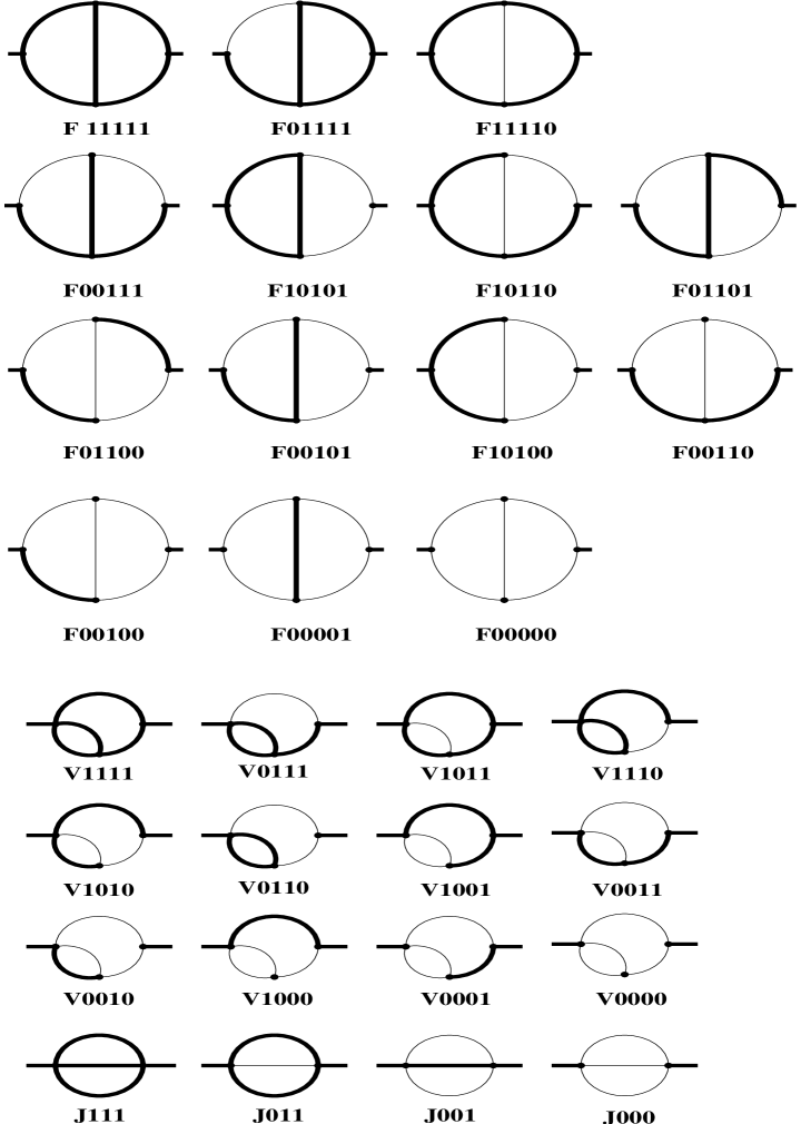
Figure 2: The full set of two-loop self-energies diagrams with one mass. Bold and thin lines correspond to the mass and massless propagators, respectively.

We consider here the following master-integrals in Euclidean space-time with dimension $D=4-2\varepsilon$:

$${\bf ONS}\{{\cal IJ}\}(i,j,m) \equiv K^{-1}\int d^{D}kP^{(i)}(k,{\cal I}m)\left.P^{(j)}(k-p,{\cal J}m)\right|_{p^{2}=-m^{2}},$$

$${\bf J}\{{\cal IJK}\}(i,j,k,m) \equiv K^{-2}\int d^{D}k_{1}d^{D}k_{2}P^{(i)}(k_{1},{\cal I}m)P^{(j)}(k_{1}-k_{2},{\cal J}m)\left.P^{(k)}(k_{2}-p,{\cal K}m)\right|_{p^{2}=-m^{2}},$$

$${\bf V}\{{\cal IJKL}\}(i,j,k,l,m) \equiv K^{-2}\int d^{D}k_{1}d^{D}k_{2}P^{(i)}(k_{2}-p,{\cal I}m)$$

$$\times P^{(j)}(k_{1}-k_{2},{\cal J}m)P^{(k)}(k_{1},{\cal K}m)\left.P^{(l)}(k_{2},{\cal L}m)\right|_{p^{2}=-m^{2}},$$

$${\bf F}\{{\cal ABIJK}\}(a,b,i,j,k,m) \equiv m^{2}K^{-2}\int d^{D}k_{1}d^{D}k_{2}P^{(a)}(k_{1},{\cal A}m)P^{(b)}(k_{2},{\cal B}m)$$

$$\times P^{(i)}(k_{1}-p,{\cal I}m)P^{(j)}(k_{2}-p,{\cal J}m)\left.P^{(k)}(k_{1}-k_{2},{\cal K}m)\right|_{p^{2}=-m^{2}},$$

where

$$K=\frac{\Gamma(1+\varepsilon)}{\left(4\pi\right)^{\frac{D}{2}}\left(m^{2}\right)^{\varepsilon}},~{}~{}~{}P^{(l)}(k,m)\equiv\frac{1}{(k^{2}+m^{2})^{l}},$$

the normalization factor $1/(2\pi)^{D}$ for each loop is assumed, and ${\cal A,B,I,J,K}=0,1.$

The finite part of most of the F-type master-integrals can be obtained from results of Ref.[9] in the limit $z\rightarrow 1$. F10101 and F11111 have been calculated in Refs.[17, 18], respectively. Instead of the usually taken F01101 integral [17, 19] we consider J111 as master integral. We recall the results of all master integrals for completeness. The last master integral F00111 has been found in [12].

The finite part of the integrals of V- and J-type can be found in Refs.[20]. The calculation of the $\varepsilon$ e ($\varepsilon^{2}$) parts of master integrals of this type have been performed by DEM.

The results for F-type master-integrals are follows:

$${\bf F}\{{\cal ABIJK}\}(1,1,1,1,1,m)=a_{1}\zeta(3)+a_{2}\frac{\pi}{\sqrt{3}}S_{2}+a_{3}i\pi\zeta(2)+{\cal O}(\varepsilon),$$ (3)

and the coefficients $\{a_{i}\}$ are given in Table I:

$$\begin{array}[]{|c|c|c|c|c|c|c|c|c|}\hline\cr\vrule\lx@intercol\hfil TABLE~{}~{}~{}I\hfil\lx@intercol\vrule\lx@intercol\\ \hline\cr&{\bf F11111}&{\bf F00111}&{\bf F10101}&{\bf F10110}&{\bf F01100}&{\bf F00101}&{\bf F10100}&{\bf F00001}\\[8.5359pt] \hline\cr a_{1}&-1&0&-4&-1&0&-3&-2&-3\\[8.5359pt] \hline\cr a_{2}&\frac{9}{2}&9&\frac{27}{2}&9&\frac{27}{2}&\frac{27}{2}&9&0\\[8.5359pt] \hline\cr a_{3}&0&0&\frac{1}{3}&0&1&1&\frac{2}{3}&1\\[8.5359pt] \hline\cr\end{array}$$

where [21, 17, 15]

$$S_{2}=\frac{4}{9\sqrt{3}}{\rm Cl}_{2}\left(\frac{\pi}{3}\right)=0.260434137632\cdots.$$

Here we used the $m^{2}-i\varepsilon$ prescription. The results for the remaining master integrals are the following ones:

$${\bf V}\{{\cal IJKL}\}(1,1,1,1,m) = \frac{1}{2\varepsilon^{2}}+\frac{1}{\varepsilon}\left(\frac{5}{2}-\frac{\pi}{\sqrt{3}}\right)+\frac{19}{2}+\frac{b_{1}}{2}\zeta(2)-4\frac{\pi}{\sqrt{3}}-\frac{63}{4}S_{2}+\frac{\pi}{\sqrt{3}}\ln 3$$

$$+ \hskip-8.0pt\varepsilon\Biggl{\{}\frac{65}{2}+b_{2}\zeta(2)-b_{3}\zeta(3)-12\frac{\pi}{\sqrt{3}}-63S_{2}+b_{4}\zeta(2)\ln 3+\frac{9}{4}b_{4}S_{2}\frac{\pi}{\sqrt{3}}$$

$$+ \frac{63}{4}S_{2}\ln 3+4\frac{\pi}{\sqrt{3}}\ln 3-\frac{1}{2}\frac{\pi}{\sqrt{3}}\ln^{2}3-\frac{b_{5}}{2}\frac{\pi}{\sqrt{3}}\zeta(2)-\frac{21}{2}\frac{{\rm Ls}_{3}\left(\frac{2\pi}{3}\right)}{\sqrt{3}}\Biggr{\}}+{\cal O}(\varepsilon^{2}),$$

where the coefficients $\{b_{i}\}$ are listen in Table II :

$$\begin{array}[]{|c|c|c|c|c|c|}\hline\cr\vrule\lx@intercol\hfil TABLE~{}~{}~{}II\hfil\lx@intercol\vrule\lx@intercol\\ \hline\cr&b_{1}&b_{2}&b_{3}&b_{4}&b_{5}\\[8.5359pt] \hline\cr{\bf V1111}&-1&-6&\frac{9}{2}&4&9\\[8.5359pt] \hline\cr{\bf V1001}&3&8&-\frac{3}{2}&0&21\\[8.5359pt] \hline\cr\end{array}$$

$${\bf J111}(1,1,1,m) = -m^{2}\Biggl{(}\frac{3}{2\varepsilon^{2}}+\frac{17}{4\varepsilon}+\frac{59}{8}+\varepsilon\Biggl{\{}\frac{65}{16}+8\zeta(2)\Biggr{\}}$$ (4)

$$- -\varepsilon^{2}\Biggl{\{}\frac{1117}{32}-52\zeta(2)+48\zeta(2)\ln 2-28\zeta(3)\Biggr{\}}+{\cal O}(\varepsilon^{3})\Biggr{)},$$

$${\bf J011}(1,1,2,m) = \frac{1-4\varepsilon}{2(1-2\varepsilon)(1-3\varepsilon)}\Biggl{(}\frac{1}{\varepsilon^{2}}+2\frac{\pi}{\sqrt{3}}-\frac{2}{3}\zeta(2)$$ (5)

$$+ \varepsilon\Biggl{\{}8\frac{\pi}{\sqrt{3}}-\frac{2}{3}\zeta(2)-6\frac{\pi}{\sqrt{3}}\ln 3+\frac{2}{3}\zeta(3)+27S_{2}\Biggr{\}}+{\cal O}(\varepsilon^{2})\Biggr{)},$$

$${\bf J011}(1,1,1,m) = -\frac{m^{2}}{2}\frac{4-15\varepsilon}{(1-2\varepsilon)(1-3\varepsilon)(2-3\varepsilon)}\Biggl{(}\frac{1}{\varepsilon^{2}}+\frac{3}{2}\frac{\pi}{\sqrt{3}}+\varepsilon\Biggl{\{}\frac{45}{8}\frac{\pi}{\sqrt{3}}-\frac{9}{2}\frac{\pi}{\sqrt{3}}\ln 3+\frac{81}{4}S_{2}\Biggr{\}}$$ (6)

$$+ \varepsilon^{2}\Biggl{\{}12-\zeta(2)-\frac{1863}{16}S_{2}-\frac{867}{32}\frac{\pi}{\sqrt{3}}+\frac{207}{8}\frac{\pi}{\sqrt{3}}\ln 3+\frac{243}{4}S_{2}\ln 3$$

$$- \frac{27}{4}\frac{\pi}{\sqrt{3}}\ln^{2}3-21\frac{\pi}{\sqrt{3}}\zeta(2)-\frac{81}{2}\frac{{\rm Ls}_{3}\left(\frac{2\pi}{3}\right)}{\sqrt{3}}\Biggr{\}}+{\cal O}(\varepsilon^{3})\Biggr{)},$$

$${\bf ONS11}(1,1,m) = \frac{1}{1-2\varepsilon}\Biggl{[}\frac{1}{\varepsilon}-\frac{\pi}{\sqrt{3}}+\varepsilon\left\{\frac{\pi}{\sqrt{3}}\ln 3-9S_{2}\right\}$$ (7)

$$+ \varepsilon^{2}\left\{9S_{2}\ln 3-\frac{1}{2}\frac{\pi}{\sqrt{3}}\ln^{2}3-6\frac{{\rm Ls}_{3}\left(\frac{2\pi}{3}\right)}{\sqrt{3}}-3\frac{\pi}{\sqrt{3}}\zeta(2)\right\}+{\cal O}(\varepsilon^{3})\Biggr{]},$$

where [15]

$${\rm Ls}_{3}(x)=-\int_{0}^{x}\ln^{2}\left|2\sin\frac{\theta}{2}\right|d\theta~{}~{}\mbox{ and }~{}~{}{\rm Ls}_{3}\left(\frac{2\pi}{3}\right)=-2.14476721256949\cdots$$

The above results were checked numerically. Padé approximants were calculated from the small momentum Taylor expansion of the diagrams [23]. The Taylor coefficients were obtained by means of the package [24] with the master integrals taken from [25]. Further we made use of the idea of Broadhurst [26] to apply the FORTRAN program PSLQ [27] to express the obtained numerical values in terms of a ‘basis’ of irrational numbers, which were predicted by DEM.

Let us point out that the numbers we obtain are related to polylogarithms at the sixth root of unity and hence are in the same class of transcendentals obtained by Broadhurst [26] in his investigation of three-loop diagrams which correspond to a closure of the two-loop topologies considered here.

Acknowledgments. Author would like to express his sincerely thanks to the Organizing Committees of the Research Workshop “Calculations for modern and future Colliders” and the XVth International Workshop “High Energy Physics and Quantum Field Theory” and especially to E.E. Boss, V.A. Ilyin, D.I. Kazakov and D.V. Shirkov for the kind invitation, the financial support at such remarkable Conferences, and for fruitful discussions. Author was supported in part by Alexander von Humboldt fellowship.

References

• [1] A.V. Kotikov, Phys.Lett. B254 (1991) 158; Mod.Phys.Lett. A6 (1991) 677.
• [2] A.V. Kotikov, Phys.Lett. B259 (1991) 314; Mod.Phys.Lett. A6 (1991) 3133.
• [3] A.V. Kotikov, Phys.Lett. B267 (1991) 123; B295 (1992) 409(E); Int.J.Mod.Phys. A6 (1992) 1977.
• [4] A.V. Kotikov, JHEP 9809 (1998) 001; in: AIHENP 93, Proceedings of the 3th International Workshop on Software Engineering, Artificial Intelligence and Expert Systems, ed.by D. Perret-Gallix, in pp. 539-544; in: ACAT 2000, Proceedings of the 7th International Workshop on Software Engineering, Artificial Intelligence and Expert Systems, ed.by D. Perret-Gallix, in American Institute of Physics Press., (hep-ph/0011316).
• [5] F.V. Tkachov, Phys.Lett. B100 (1981) 65; K.G. Chetyrkin and F.V. Tkachov, Nucl.Phys. B192 (1981) 159; A.N. Vassiliev, Yu.M. Pis’mak and Yu.R. Khonkonen, Theor.Math.Phys. B47 (1981) 465.
• [6] C. Ford, I. Jack and D.R.T. Jones, Nucl.Phys. B387 (1992) 373.
• [7] J. Fleischer, M. Tentyukov, and O.V. Tarasov, Nucl.Phys.Proc.Suppl. 89 (2000) 112.
• [8] E. Remiddi, Nuovo Cim. A110 (1997) 1435.
• [9] J. Fleischer, A.V. Kotikov, and O.L. Veretin, Nucl.Phys. B547 (1999) 343.
• [10] J. Fleischer, A.V. Kotikov, and O.L. Veretin, Phys.Lett. B417 (1998) 163.
• [11] J. Fleischer, A.V. Kotikov, and O.L. Veretin, Acta Phys.Polon. B29 (1998) 2611.
• [12] J. Fleischer, M.Yu. Kalmykov, and A.V. Kotikov, Phys.Lett. B462 (1999) 169; B467 (1999) 310(E).
• [13] J. Fleischer, M.Yu. Kalmykov, and A.V. Kotikov, in AIHENP 99, Proceedings of the 6th International Workshop on Software Engineering, Artificial Intelligence and Expert Systems, ed.by G. Athanasiu and D. Perret-Gallix, in Parisianou S.A., Athens, 2000, pp. 231-237, (hep-ph/9905379); J. Fleischer and M.Yu. Kalmykov, Comput.Phys.Commun. 128 (2000) 531.
• [14] T. Gehrmann and E. Remiddi, Nucl.Phys. B580 (2000) 485; Preprint TTP00-20, 2000 (hep-ph/0008287); Preprint CERN-TH/2001-005, 2001 (hep-ph/0101124); Preprint TTP01-04, 2001 (hep-ph/0101147); Nucl.Phys.Proc.Suppl. 89 (2000) 251; C. Anastasiou, T. Gehrmann, C. Oleari, E. Remiddi and J.B. Tausk, Nucl.Phys. B580 (2000) 577.
• [15] L. Lewin, Polylogarithms and Associated Functions, North Holland, New-York, 1981.
• [16] D.I. Kazakov and A.V. Kotikov, Theor.Math.Phys. 73 (1987) 1264; Nucl.Phys. B307 (1988) 721; B345 (1990) 299(E); Phys.Lett. B291 (1992) 171; A.V. Kotikov, Theor.Math.Phys. 78 (1989) 134.
• [17] D.J. Broadhurst, Z.Phys. C47 (1990) 115.
• [18] V. Borodulin and G. Jikia, Phys.Lett. B391 (1997) 434.
• [19] N. Gray, D.J. Broadhurst, W. Grafe and K. Schilcher, Z.Phys. C48 (1990) 673; D.J. Broadhurst, N. Gray and K. Schilcher, Z.Phys. C52 (1991) 111; D.J. Broadhurst, Z.Phys. C54 (1992) 599.
• [20] A. Djouadi, Nuovo Cim. A100 (1988) 357; P.N. Maher, L. Durand and K.Riesselmann, Phys.Rev. D48 (1993) 1061; D52 (1995) 553(E); R. Scharf and J.B. Tausk, Nucl.Phys. B412 (1994) 523; F.A. Berends, M. Buza, M. Böhm and R. Scharf, Z.Phys. C63 (1994) 227; F.A. Berends and J.B. Tausk, Nucl.Phys. B421 (1994) 456; S. Bauberger, F.A. Berends, M. Böhm and M. Buza, Nucl.Phys. B434 (1995) 383.
• [21] J. van der Bij and M. Veltman, Nucl.Phys. B231 (1984) 205; F. Hoogeveen, Nucl.Phys. B259 (1985) 19; J. van der Bij and F. Hoogeveen, Nucl.Phys. B283 (1987) 477.
• [22] A.I. Davydychev and M.Yu. Kalmykov, Preprint MZ-TH/00-52, 2000, (hep-th/0012189).
• [23] J. Fleischer and O.V. Tarasov, Z.Phys. C64 (1994) 413; O.V. Tarasov, Nucl.Phys. B480 (1996) 397.
• [24] L.V. Avdeev, J. Fleischer, M.Yu. Kalmykov and M.N. Tentyukov, Nucl.Inst.Meth. A389 (1997) 343; Comp.Phys.Commun. 107 (1997) 155.
• [25] A.I. Davydychev and J.B. Tausk, Nucl.Phys. B397 (1993) 123.
• [26] D.J. Broadhurst, Eur.Phys.J. C8 (1999) 311.
• [27] H.R.P. Ferguson, D.H. Bailey and S. Arno, NASA-Ames Technical Report, NAS-96-005; D.H. Bailey and D.J. Broadhurst, math.NA/9905048.
• [28] D.J. Broadhurst, J.A. Gracey, and D. Kreimer, Z.Phys. C75 (1997) 559; D.J. Broadhurst and A.V. Kotikov, Phys.Lett. B441 (1998) 345; A.V. Kotikov and L.N. Lipatov, Nucl.Phys. B582 (2000) 19; A.V. Kotikov, in: Proceedings of the XVth International Workshop “High Energy Physics and Quantum Field Theory“  (hep-ph/0102177).