ANL-HEP-PR-01-007 EFI-2001-004 FERMILAB-PUB-01/014-T IFT-00/31 IEM-FT-207/00 IFT-UAM/CSIC-00-41 Brane Effects on Extra Dimensional Scenarios:
A Tale of Two Gravitons

Abstract

We analyze the propagation of a scalar field in multidimensional theories which include kinetic corrections in the brane, as a prototype for gravitational interactions in a four dimensional brane located in a (nearly) flat extra dimensional bulk. We regularize the theory by introducing an infrared cutoff given by the size of the extra dimensions and a physical ultraviolet cutoff of the order of the fundamental Planck scale in the higher dimensional theory. We show that, contrary to recent suggestions, the radius of the extra dimensions cannot be arbitrarily large. Moreover, for finite radii, the gravitational effects localized on the brane can substantially alter the phenomenology of collider and/or table-top gravitational experiments. This phenomenology is dictated by the presence of a massless graviton, with standard couplings to the matter fields, and a massive graviton which couples to matter in a much stronger way. While graviton KK modes lighter than the massive graviton couple to matter in a standard way, the couplings to matter of the heavier KK modes are strongly suppressed.

1 Introduction

The existence of large extra dimensions, of size much larger than the Planck length, has been recently proposed by Arkani-Hamed, Dimopoulos and Dvali (ADD) [1] as an alternative means of solving the hierarchy problem of the Standard Model (SM). It has been argued that, if the SM fields were localized in a four dimensional brane located in a compact flat spatial bulk of radius $R$, which allows the free propagation of gravitons, the physical Planck scale associated with the gravity properties at distances much larger than $R$ will be given by $M_{Pl}^{2}=M^{2+d}R^{d}$, where $M$ is the fundamental Planck scale and $d$ is the number of extra dimensions. For this mechanism to provide a solution of the hierarchy problem, $M$ should be on the order of a TeV. Since gravity will look ($4+d$) dimensional at distances much shorter than $R$, the compactification radius cannot be larger than a millimeter. While such a bound is inconsistent with a solution to the hierarchy problem in the case $d=1$, it is naturally fulfilled for $d\geq 2$. The smaller $d$, the larger becomes $R$ and, for $d=2$, the predicted deviation of the gravity behavior is being tested in table-top experiments [2, 3].

Since the fundamental scale $M$ is of order a TeV, non-trivial modifications will also appear in the ultraviolet regime of energies close to $M$. From a four dimensional point of view, the ultraviolet effects will be associated with the emission of Kaluza-Klein (KK) states, representing the propagation of the graviton in the extra dimensional bulk. Although individual KK gravitons will couple very weakly to SM particles, the cumulative effect of KK gravitons will lead to interactions which become strong at energy scales of order $M$. For collider center-of-mass energies approaching $M$, graviton emission can be observed as missing energy signatures, or as virtual effects that interfere with SM processes [4]. Nonobservation of these collider effects places a lower bound on $M$ of about a TeV.

From the above considerations, it seems clear that, for a compact flat bulk space, $R$ cannot be larger than a millimeter without producing gross deviations from four dimensional gravity at macroscopic scales. This point of view has been recently challenged by the authors of Ref. [5]. They show that, if $d=1$ and $R$ is taken to be infinitely large, the possible inclusion of a local four dimensional Einstein term in the brane (see also [6]) may lead to short–distance behavior that resembles the usual four dimensional propagation of gravitons. Moreover, in Ref. [7] it was argued that if the number of dimensions is larger than five, $d\geq 2$, one obtains four dimensional behavior for the graviton at all scales. However, for $d\geq 2$ this result is derived from expressions involving an ultraviolet divergent contribution coming from the propagation of gravitons in the bulk, and therefore the case $d\geq 2$ deserves a more detailed analysis. This is particularly so since we are considering a non-renormalizable theory with a physical ultraviolet cutoff which cannot be larger than the ($4+d$) dimensional Planck scale $M$, at which gravity interactions in the extra dimensional bulk become strong.

In this paper we will introduce both an infrared (IR) and an ultraviolet (UV) regularization. The IR regularization is implemented by means of a $d$ dimensional torus with common radius $R$. We introduce a physical UV cutoff $\Lambda$ by truncating the number of KK-modes at $|\vec{n}|=\Lambda R/\pi$, where $\vec{n}^{2}=n_{1}^{2}+\cdots n_{d}^{2}$. The case of $(4+d)$ dimensional Minkowski space considered in Refs. [5, 7] will appear as the $R\to\infty$ limit. In this limit we will reproduce the results of Ref. [5] for the case of one extra dimension; moreover for $d\geq 2$ we reproduce the results of Ref. [7] in the limit $R\to\infty$ and $\Lambda\to\infty$. However, when we fix the UV cutoff to a natural physical value $\mathcal{O}(M)$, the results we obtain are different from those obtained in [7].

For the case of finite radius (toroidal) extra dimensions the presence of brane gravitational corrections could substantially modify the usual ADD scenario. In fact we shall show that, depending on the strength of those corrections, either the collider or table-top gravitational signatures can be substantially altered.

The outline of this paper is as follows. In section 2 we study the structure of the bulk graviton propagator including the brane corrections for an arbitrary number of flat extra dimensions. In section 3 we consider the $R\to\infty$ limit to compare with the results of Refs. [5, 7]. In section 4 we consider the case of finite radius and analyze the physical features of the relevant momentum (or distance) regimes. Section 5 is devoted to the phenomenology, including collider experiments and gravitational table-top experiments. Finally our conclusions and outlook are presented in section 6 and some lengthy formulae are exhibited in appendix A.

2 General propagator including the brane correction

We start with a $(4+d)$ dimensional theory with coordinates $x^{I}\equiv(x^{\mu},y^{i})$, where $x^{\mu}$ are the four dimensional space-time coordinates and $0\leq\,y^{i}\,\leq R$, ($i=1,\dots,d$) those of the compact space and assume a 3-brane embedded in the $(4+d)$ dimensional space at $y=0$. We shall assume that the brane thickness is small compared to the $(4+d)$ dimensional Planck length, and model it by a delta function in the extra dimensions. Following Refs. [5, 7], we shall consider, for simplicity, a single bulk scalar field $\phi(x^{I})$, instead of the more complicated tensor structure of a graviton, propagating in the $(4+d)$ dimensional space, with the action:

$$S_{4+d}=\int d^{4}xd^{d}y\left\{M^{2+d}\partial_{I}\phi(x,y)\partial^{I}\phi(x,y)+\bar{M}^{2}\delta(y)\partial_{\mu}\phi(x,0)\partial^{\mu}\phi(x,0)\right\}$$ (2.1)

where $M$ is the higher dimensional Planck scale, $\bar{M}$ is the coefficient of the brane-generated correction, and we have scaled the $\phi$ field to be dimensionless. Eq. (2.1) should be regarded as the leading terms in a bulk+brane effective action for dynamics in a $(4+d)$ dimensional flat space background (we are ignoring bulk+brane cosmological constant terms). The effective action will be valid up to some physical ultraviolet cutoff $\Lambda$, where it matches onto a more fundamental UV description. Since bulk gravity becomes strongly interacting at the energy scale $M$, we expect that the case of interest is $\Lambda$ not much larger than $M$.

The brane-generated kinetic term with coefficient $\bar{M}$ could be induced from the coupling between bulk gravity (the bulk scalar, in our simplified treatment) and the brane matter fields. As noted in [5, 7], graviton vacuum polarization diagrams with brane matter loops will generically produce such a term. For example, if there are $N$ heavy brane particles of mass $m$, they will generate a contribution to $\bar{M}$ on the order of $Nm^{2}$ times a loop factor [8]-[11]. Even in an effective theory with a cutoff $\Lambda\simeq M$, it is consistent to imagine that $\bar{M}$ may be much larger than $M$. This occurs in the example above if $N$ is large; it could also arise from dynamical sources such as coupling to brane or bulk fields which have large vacuum expectation values. Other possibilities include a large $\bar{M}$ related to physics of the fundamental UV theory. On the other hand $\bar{M}\gg M$ introduces a hierarchy problem, which would have to be addressed in a complete model.

We are interested in obtaining the Green function for the propagation of the scalar field from a point in the brane to any point in the $(4+d)$ dimensional space. The equation for the corresponding Green function, after making a Fourier transform over the four dimensional space-time coordinates, is

$$[M^{2+d}(p^{2}-\Delta_{d})+\bar{M}^{2}p^{2}\delta^{(d)}(y_{i})]G_{d}(p,y_{i})=\delta^{(d)}(y_{i})$$ (2.2)

where $p^{2}=p_{1}^{2}+p_{2}^{2}+p_{3}^{2}+p_{4}^{2}$ is the four dimensional euclidean momentum and $\Delta_{d}$ is the laplacian operator in $d$ dimensions.

The solution to Eq. (2.2) can be written as follows, [5, 7]:

$$G_{d}(p,y_{i})=\frac{D_{d}(p,y_{i})}{M^{2+d}+\bar{M}^{2}p^{2}D_{d}(p,0)}$$ (2.3)

where $D_{d}(p,y_{i})$ is the solution to the equation

$$(p^{2}-\Delta_{d})D_{d}(p,y_{i})=\delta^{(d)}(y_{i})\ .$$ (2.4)

A way to solve Eq. (2.4) is by Fourier series, since the extra dimensions are finite. We will only be interested in the behavior of the higher dimensional propagator on the 3-brane, that is for $y_{i}=0$. In this case the form for $D_{d}(p,0)$ is just the sum

$$D_{d}(p,0)=\frac{1}{R^{d}}\sum_{\vec{n}}\frac{1}{p^{2}+\frac{\vec{n}^{2}\pi^{2}}{R^{2}}}$$ (2.5)

where the vector $\vec{n}$ is defined as, $\vec{n}=(n_{1},\dots,n_{d})$.

The Green function on the 3-brane $G_{d}(p,0)$ could also be obtained after integration of the action (2.1) over the extra dimensional coordinates $y^{i}$, which yields the four dimensional Lagrangian for the KK-states $\phi^{(\vec{n})}$,

$$\mathcal{L}_{4}=M^{2+d}\,R^{d}\sum_{\vec{n}}\left(\partial_{\mu}\phi^{(\vec{n})}\partial^{\mu}\phi^{(\vec{n})}-\frac{\vec{n}^{2}}{R^{2}}\,\phi^{(\vec{n})}\phi^{(\vec{n})}\right)+\bar{M}^{2}\sum_{\vec{n},\,\vec{m}}\partial_{\mu}\phi^{(\vec{n})}\partial^{\mu}\phi^{(\vec{m})}\ .$$ (2.6)

The Green function on the 3-brane is the sum over four dimensional propagators. To compute it we consider the first two terms in (2.6) as the unperturbed Lagrangian, giving rise to the sum

${\displaystyle D_{d}(p,0)/M^{2+d}=\sum_{\vec{n}}\quad(\vec{n})}$ \begin{picture}(70.0,30.0)(0.0,28.0) \put(0.0,0.0){} \end{picture}$(\vec{n})\equiv$

and the last term as the perturbed Lagrangian, giving rise to the mixing

$-\,p^{2}\,\bar{M}^{2}\equiv\quad(\vec{n})$ \begin{picture}(70.0,30.0)(0.0,28.0) \put(0.0,0.0){} \put(0.0,0.0){} \put(0.0,0.0){} \end{picture}      $(\vec{m})$

In this way the complete Green function $G_{d}(p,0)$ can be computed as

$G_{d}(p,0)\equiv$ \begin{picture}(50.0,30.0)(0.0,28.0) \put(0.0,0.0){} \end{picture} + \begin{picture}(50.0,30.0)(0.0,28.0) \put(0.0,0.0){} \put(0.0,0.0){} \put(0.0,0.0){} \end{picture}              + \begin{picture}(50.0,30.0)(0.0,28.0) \put(0.0,0.0){} \put(0.0,0.0){} \put(0.0,0.0){} \put(0.0,0.0){} \put(0.0,0.0){} \end{picture}$\hskip 71.13188pt+\quad\cdots$

and coincides with the expression obtained from (2.3) and (2.5).

We have computed the sum over the four dimensional propagators in the original field basis, without explicitly diagonalizing the lagrangian (2.6). In the basis of canonically normalized mass eigenstates for the lagrangian (2.6), $G_{d}(p,0)$ is just the sum over the exact KK propagators, with mode dependent residues proportional to the square of the coupling of the corresponding eigenstates to matter, whereas $D_{d}(p,0)$ is the sum over the unperturbed KK propagators.

In principle the summation is over all KK modes, but since the action (2.1) is that of an effective theory we should cutoff the sum when the mass of the modes are of order of the scale $\Lambda$, where $\Lambda$ is the cutoff of the theory. That is we will sum up to a maximum $\vec{n}^{2}_{\rm max}=(\Lambda R/\pi)^{2}$. We expect the cutoff $\Lambda$ to be of the order of the characteristic scale of the underlying higher dimensional theory.

For large values of $R$, as those that we will be interested in this paper, we can approximate the summation in (2.5) by an integral over the $n_{i}$. After subtracting the zero-mode we can write (2.5) as,

$$D_{d}(p,0)=\frac{1}{p^{2}R^{d}}\left(1+\Omega_{d}\frac{R^{d}p^{d}}{\pi^{d}}\int_{\frac{\pi}{Rp}}^{\frac{\Lambda}{p}}\frac{x^{d-1}dx}{1+x^{2}}\right)$$ (2.7)

where $\Omega_{d}=\frac{2\pi^{d/2}}{2^{d}\Gamma[\frac{d}{2}]}$ is the solid angle sustained in $d$ dimensions for $y_{i}>0$. This expression can be considered as the $y_{i}\to 0$ limit of the bulk propagator

$$D_{d}(p,y)=\frac{1}{p^{2}R^{d}}\left(1+\left(\frac{\pi}{2}\right)^{\frac{d}{2}}\frac{R^{d}p^{d}}{\pi^{d}}\int_{\frac{\pi}{Rp}}^{\frac{\Lambda}{p}}\frac{x^{d-1}\;J_{d/2-1}(xpy)\;dx}{(xpy)^{d/2-1}(1+x^{2})}\right)$$ (2.8)

where the $J_{d/2-1}$ are Bessel functions and $y\equiv|\vec{y}|$.

The explicit expressions for the Green functions $D_{d}(p,0)$ are given in Appendix A, Eqs. (A.1) and (A.2), as well as their analytic continuation into the Minkowski space-time, $D_{d}(s)$, Eqs. (A.3) and (A.4). For the purpose of this paper we will find it more convenient to work in Minkowski space-time so we will use, from here on,‘ the Green functions $D_{d}(s)$, as given by (A.3) and (A.4) as well as the corresponding $G_{d}(s)$ functions as defined by

$$G_{d}(s)=\frac{D_{d}(s)}{M^{2+d}-\bar{M}^{2}sD_{d}(s)}\ .$$ (2.9)

The cases where $d=1$, $2$ are particularly interesting, and they will be analyzed separately in the following sections. The corresponding Green functions, within the approximation given in Eq. (2.7), can be written as:

$$G_{1}(s)={\displaystyle\frac{-1+\frac{R\sqrt{s}}{\pi}\left[i\,\frac{\pi}{2}-\tanh^{-1}\left(\frac{\sqrt{s}}{\Lambda}\right)+\tanh^{-1}\left(\frac{\pi}{R\sqrt{s}}\right)\right]}{\left(M^{3}R+\bar{M}^{2}\right)s-\frac{\bar{M}^{2}R\,s\sqrt{s}}{\pi}\left[i\,\frac{\pi}{2}-\tanh^{-1}\left(\frac{\sqrt{s}}{\Lambda}\right)+\tanh^{-1}\left(\frac{\pi}{R\sqrt{s}}\right)\right]}}$$ (2.10)

and

$$G_{2}(s)={\displaystyle\frac{-1+\frac{R^{2}\,s}{2\pi}\,\left[i\,\frac{\pi}{2}+\frac{1}{2}\log\left(\frac{\Lambda^{2}}{s}-1\right)-\frac{1}{2}\log\left(1-\frac{\pi^{2}}{R^{2}s}\right)\right]}{\left(M^{4}R^{2}+\bar{M}^{2}\right)s-\frac{\bar{M}^{2}R^{2}s^{2}}{2\,\pi}\,\left[i\,\frac{\pi}{2}+\frac{1}{2}\log\left(\frac{\Lambda^{2}}{s}-1\right)-\frac{1}{2}\log\left(1-\frac{\pi^{2}}{R^{2}s}\right)\right]}}\ .$$ (2.11)

We are now ready to study the behavior of the Green functions in the different regimes of values for $R$ and, in particular, the impact on them of the presence of the brane corrections proportional to $\bar{M}$.

3 The limit of infinite size extra dimensions

In this section we will analyze the behavior of the theory for extremely large values of the radius $R$ and, in particular, its behavior in the $R\to\infty$ limit, that has been recently proposed as an alternative way of localizing gravity in the 3-brane. We will make a separate analysis of the five and six dimensional cases and then we will analyze the general case for $d>2$.

3.1 One extra dimension

The Green function (2.10) in the $R\to\infty$ limit is given by,

$$G_{1}(s)\simeq\frac{i\,\frac{\pi}{2}-\tanh^{-1}\left(\frac{\sqrt{s}}{\Lambda}\right)}{\pi\,M^{3}\sqrt{s}-\bar{M}^{2}\,s\left[\frac{i\,\pi}{2}-\tanh^{-1}\left(\frac{\sqrt{s}}{\Lambda}\right)\right]}\ .$$ (3.1)

In the region ($\sqrt{s}\ll\Lambda$), $\tanh^{-1}(\sqrt{s}/\Lambda)\simeq\sqrt{s}/\Lambda$ and the Green function (3.1) behaves approximately as,

$$G_{1}(s)\simeq-\frac{1}{i\,2\,M^{3}\,\sqrt{s}+\bar{M}^{2}\,s}\ .$$ (3.2)

We reproduce in this way the propagator found in Ref. [5] for the case of one infinite flat extra dimension. The physics described by (3.2) was already analyzed in Ref. [5]. For distances $r\gg r_{c}$, where the critical distance is given by $r_{c}\simeq\bar{M}^{2}/2\,M^{3}$ the linear term ($\sqrt{s}$-term) in (3.2) dominates and the propagator behaves as a five dimensional one. However, as already observed in Ref. [5], even for the most favorable case of $\bar{M}\simeq M_{Pl}$ and $M\simeq 1$ TeV, the critical distance is not large enough, $r_{c}\simeq 10^{15}$ cm, and enters in conflict with well tested Newtonian predictions. Moreover, for $r\ll r_{c}$ the quadratic term in (3.2) (corresponding to a four dimensional theory with a propagator $\sim-1/\bar{M}^{2}s$), dominates but the theory is described by a scalar-tensor theory of gravity, with an additional scalar attractive force corresponding to the five degrees of freedom of a 4D massive or 5D massless graviton.

3.2 Two extra dimensions

A similar analysis can be done for the $d=2$ case using the Green function (2.11). The $R\to\infty$ limit of (2.11) is,

$$G_{2}(s)\simeq\frac{i\,\pi+\log\left(\Lambda^{2}/s\right)}{4\pi\,M^{4}-\bar{M}^{2}\,s\left[i\,\pi+\log\left(\Lambda^{2}/s\right)\right]}\ .$$ (3.3)

Should we take the limit of (3.3) when $\Lambda\to\infty$ we would obtain for the Green function the behavior $G_{2}(s)\sim-1/\bar{M}^{2}s$, which, in the full gravity theory, would correspond to the graviton propagator in a four dimensional tensor theory of gravity, reproducing the result in Ref. [7]. However since, as we mentioned in the previous section, $\Lambda=\mathcal{O}(M)$, in the limit $s\ll M^{2}$ we cannot neglect the constant term in the denominator of (3.3) for all momenta. As we did in the five dimensional case, we can compute the critical distance on the brane $r_{c}$ such that for $r\gg r_{c}$ the constant term dominates in the denominator of the Green function (3.3). In this region the Green function is logarithmic and as such it corresponds to the propagator in a six dimensional theory. Only for distances $r\ll r_{c}$ the quadratic term dominates, leading to the typical behaviour of the propagator in a four dimensional theory.

The value of $r_{c}$ cannot be given analytically, as in the previous case. However a good approximation is given by,

$$r_{c}\simeq\frac{\bar{M}}{M^{2}}\ \sqrt{\frac{1}{2\,\pi}\,\log\frac{\bar{M}}{M}}\equiv\frac{1}{\mathcal{M}_{2}}\ ,$$ (3.4)

where we have use that $\Lambda\simeq M$. On the other hand, for values of $s$ close to $\mathcal{M}_{2}$ the Green function (3.3) can be approximated by,

$$G_{2}(s)\simeq-\frac{1}{\bar{M}^{2}}\ \frac{1+i\gamma_{2}}{s-\mathcal{M}_{2}^{2}+is\;\gamma_{2}}$$ (3.5)

which describes the propagation of a resonance of mass $\mathcal{M}_{2}$ given by (3.4) and width governed by

$$\gamma_{2}=\frac{\pi}{2}\;\frac{1}{\log\,\bar{M}/M}\ .$$ (3.6)

Using the previous values, $\bar{M}\simeq M_{Pl}$ and $M\simeq 1$ TeV, we obtain from Eq. (3.4) $r_{c}\simeq 5$ mm, which corresponds to $\mathcal{M}_{2}\simeq 5\times 10^{-5}$ eV. This low value of $r_{c}$ is ruled out since it would imply that the gravity propagator behaves as six dimensional for $r>r_{c}$ and we know that for distances larger than sub-millimeter [2] gravity interactions are well described by four dimensional Einstein gravity.

3.3 More than two extra dimensions

For more than two extra dimensions the analysis can be done in full generality using Eqs. (A.3) and (A.4). The general propagator for $R\to\infty$ is, for $d$ odd,

$$D_{d}(s)=\frac{\Omega_{d}}{\pi^{d}}\,s^{\frac{d}{2}-1}\left[i\,\frac{\pi}{2}-\tanh^{-1}\left(\frac{\sqrt{s}}{\Lambda}\right)+\sum_{n=1}^{(d-1)/2}\frac{1}{d-2n}\left(\frac{\Lambda^{2}}{s}\right)^{\frac{d}{2}-n}\right]$$ (3.7)

and for $d$ even:

$$D_{d}(s)=\frac{\Omega_{d}}{\pi^{d}}\,s^{\frac{d}{2}-1}\left[i\,\frac{\pi}{2}+\frac{1}{2}\log\left(\frac{\Lambda^{2}}{s}-1\right)+\sum_{n=1}^{\frac{d}{2}-1}\frac{1}{d-2n}\left(\frac{\Lambda^{2}}{s}\right)^{\frac{d}{2}-n}\right]\ .$$ (3.8)

In the regime $s\ll\Lambda^{2}$ both formulae behave in the same way:

$$D_{d}(s)\simeq\omega_{d}\,\left[i\,\frac{\pi}{2}(d-2)\,s^{\frac{d}{2}-1}+\Lambda^{d-2}\right]$$ (3.9)

where $\omega_{d}$ for $d>2$ is given by

$$\omega_{d}=\frac{\Omega_{d}}{(d-2)\,\pi^{d}}\ .$$ (3.10)

Inserting the above equation into the full propagator we find:

$$G_{d}(s)\simeq-\frac{1}{\bar{M}^{2}}\;\frac{1+i\,\frac{\pi}{2}(d-2)\left(\sqrt{s}/\Lambda\right)^{d-2}}{s-\mathcal{M}_{d}^{2}+i\,\frac{\pi}{2}(d-2)s\,\left(\sqrt{s}/\Lambda\right)^{d-2}}$$ (3.11)

where $\mathcal{M}_{d}$ is defined by

$$\mathcal{M}_{d}=\frac{1}{\sqrt{\omega_{d}}}\ \frac{M^{2}}{\bar{M}}\left(M/\Lambda\right)^{d-2}\simeq\frac{1}{\sqrt{\omega_{d}}}\ \frac{M^{2}}{\bar{M}}\ .$$ (3.12)

where the last expression is valid for $\Lambda\simeq M$.

Again, as in the previous subsection, in the limit $\Lambda\to\infty$ we would obtain for the Green function the behavior $G_{2}(s)\sim-1/\bar{M}^{2}s$, corresponding to the propagator in a four dimensional tensor theory of gravitation, reproducing the results of Ref. [7]. However, since $\Lambda=\mathcal{O}(M)$, what we obtain from (3.11) corresponds to a massive resonance with a mass $\mathcal{M}_{d}$, width controlled by the function

$$\gamma_{d}(s)=\frac{\pi}{2}(d-2)\left(\frac{\sqrt{s}}{M}\right)^{d-2}$$ (3.13)

and propagator given by

$$G_{d}(s)\simeq-\frac{1}{\bar{M}^{2}}\frac{s-\mathcal{M}_{d}^{2}-s\gamma_{d}^{2}-i\,\gamma_{d}\mathcal{M}_{d}^{2}}{\left(s-\mathcal{M}_{d}^{2}\right)^{2}+s^{2}\gamma_{d}^{2}}\ .$$ (3.14)

Observe that, since we are assuming that $s\ll M^{2}$, $\gamma_{d}(s)$ may be approximately written as

$$\gamma_{d}(s)\simeq\frac{\pi}{2}\frac{(d-2)}{\left[\left(\frac{M}{\sqrt{s}}\right)^{d-2}-1\right]}$$ (3.15)

what allows to make connection with the two dimensional case.

Using again $\bar{M}\simeq M_{Pl}$ and $M\simeq 1$ TeV, we get from (3.12) $\mathcal{M}_{d}\stackrel{{\scriptstyle>}}{{{}_{\sim}}}10^{-4}$ eV. A massive graviton as in (3.14) is excluded, which leads to ruling out the scenarios [7] with infinite size extra dimensions in flat space.

Thus, from the four dimensional point view, for $d>1$ the theory has a mode, whose mass has a non-vanishing value in the $R\to\infty$ limit. As follows from Eq. (3.2), such a mode is absent for $d=1$, what is also consistent with the results in the case of finite size extra dimensions discussed in section 4.

4 The case of finite size extra dimensions

In this section we will consider the modification of the ADD scenario by the effect of brane gravitational corrections. We shall describe the Green function in the region where $\sqrt{s}\ll\Lambda$, and we shall put emphasis on the case in which the cutoff of the effective theory $\Lambda$ is identified with the higher dimensional Planck scale $M$. The physical (four dimensional) Planck mass is defined as

$$M_{Pl}^{2}=M^{d+2}R^{d}+\bar{M}^{2}\ ,$$ (4.1)

and it is associated with the interaction strength of the massless graviton appearing in the spectrum of the theory for any value of $d$. We shall always assume that $\bar{M}^{2}$ is small compared to the first term in Eq. (4.1), which proceeds from the dimensional reduction of the higher dimensional theory. We will be subsequently interested in the IR ($R\sqrt{s}\ll 1$) and UV ($R\sqrt{s}\gg 1$) regions.

4.1 The IR region

In the IR region, $R\sqrt{s}\ll 1$, the Green function $D_{d}(s)$ can be written as,

$$D_{d}(s)\simeq-\frac{1}{R^{d}\,s}+\frac{\Omega_{d}}{(d-2)\pi^{2}R^{d-2}}\left[\left(\frac{\Lambda\;R}{\pi}\right)^{d-2}-1\right]$$ (4.2)

which is valid for any dimension $d$ .

The Green function $G_{d}(s)$ behaves then as a massless particle with gravitational coupling given by $1/M_{Pl}^{2}$, which corresponds to Einstein gravity, plus a massive particle with coupling $\sim 1/\bar{M}^{2}$. In fact, we can write (2.9) as:

$$G_{d}(s)\simeq-\frac{1}{M_{Pl}^{2}\,s}-\frac{1}{\bar{M}^{2}}\left(1-\frac{\bar{M}^{2}}{M_{Pl}^{2}}\right)\,\frac{1}{s-\mathcal{M}_{d}^{2}}$$ (4.3)

with the mass $\mathcal{M}_{d}$, for $d\geq 2$, given by,

$$\mathcal{M}_{d}^{2}=\left(\frac{M}{\Lambda}\right)^{d-2}\;\frac{M^{2}}{\omega_{d}}\left(\frac{M^{2}}{\bar{M}^{2}}+\frac{1}{(RM)^{d}}\right)=\left(\frac{M}{\Lambda}\right)^{d-2}\;\frac{1}{\omega_{d}}\ \left(1-\frac{\bar{M}^{2}}{M_{Pl}^{2}}\right)^{-1}\,\frac{M^{2}}{\bar{M}^{2}}\,M^{2}\ .$$ (4.4)

The second equality comes from (4.1) with $\omega_{d}$ given in Eq. (3.10) for $d>2$, and

$$\omega_{2}=\frac{1}{2\,\pi}\log\frac{R\;\Lambda}{\pi}.$$ (4.5)

Furthermore, for $d=1$ we obtain

$$\mathcal{M}_{1}^{2}=\frac{M_{Pl}^{2}}{\bar{M}^{2}}\,\frac{\pi^{2}}{R^{2}}\ .$$ (4.6)

Eq. (4.4) shows explicitly, for $d>2$, the $R$ independent behavior of the mass, in close relation to the result for $\mathcal{M}_{d}$ in the $R\to\infty$ limit, obtained in section 3, Eq. (3.12). Eq. (4.6) shows that such a pole does not appear in the infrared regime for $d=1$. For $d=2$, the value of $\mathcal{M}_{2}^{2}$ is given by

$$\mathcal{M}_{2}^{2}=\frac{M_{Pl}^{2}}{\bar{M}^{2}}\,\frac{1}{\omega_{2}\;R^{2}}\ .$$ (4.7)

and hence, from the expression of $\omega_{2}$ (4.5), and excluding the unphysical case $\Lambda\gg M$, we obtain that, unless $\bar{M}$ is of order $M_{Pl}$, such a state will also be absent in the infrared regime.

Since for $d=1$ the mass term (4.6) is, for $\bar{M}^{2}\ll M_{Pl}^{2}$, much larger than $1/R$, the second term in (4.3) corresponds, in the IR region, to a contact term in the propagator. A similar effect is obtained for $d=2$. For $d>2$, instead, the second term in (4.3) corresponds to a massive state coupled with a strength $1/\bar{M}^{2}$. This state will appear in the physical spectrum of the theory whenever $\mathcal{M}_{d}$ is in the energy range under consideration, namely whenever $\mathcal{M}_{d}<1/R$. This happens, for $M\simeq\Lambda$, when

$$\left(1-\frac{\bar{M}^{2}}{M_{Pl}^{2}}\right)^{\frac{1}{2}-\frac{1}{d}}\bar{M}>\sqrt{\frac{1}{\omega_{d}}}\,\left(\frac{M_{Pl}}{M}\right)^{2/d}M\simeq\sqrt{\frac{1}{\omega_{d}}}\,10^{\,32/d}\,\left(\frac{\rm 1\,TeV}{M}\right)^{2/d}\,M\ .$$ (4.8)

As noticed above, the inequality (4.8) is only consistent with a coupling much stronger than the gravitational one, i.e. $\bar{M}\ll M_{Pl}$, for $d\geq 3$. In this case the second term of (4.3) gives rise to a massive “condensate” with a mass given by Eq. (4.4) and a coupling much stronger than the gravitational one. This leads to a very novel phenomenon: The presence of two gravitons in the spectrum, with masses lower than the compactification scale $1/R$. One of the gravitons becomes massless and mediates the regular gravitational interactions. The second graviton, much more strongly coupled, could have a mass in the range detectable by table-top gravitational experiments, as we will see in the next section.

4.2 The UV region

In the UV region, $R\sqrt{s}\gg 1$, the Green functions for $d=1,2$ can be taken directly from Eqs. (2.10) and (2.11). In particular for $d=1$ the Green function is,

$$G_{1}(s)\simeq-\frac{R}{i\,2\,M_{Pl}^{2}\,\sqrt{s}+\bar{M}^{2}\,R\,s}\ .$$ (4.9)

For $\sqrt{s}\gg r_{c}^{-1}$ ($\sqrt{s}\ll r_{c}^{-1}$) the theory behaves four dimensional (five dimensional), and the critical length is,

$$r_{c}\simeq\frac{\bar{M}^{2}\,R}{2\,M_{Pl}^{2}}\ .$$ (4.10)

Assuming now that $M_{Pl}^{2}\simeq M^{3}\,R$, as discussed above, we obtain from (4.10) $r_{c}\simeq\bar{M}^{2}/2\,M^{3}$, the same critical length we got in section 3 for the $R\to\infty$ case. Moreover, for $d=1$ and $\bar{M}\ll M_{Pl}$, $R\simeq 10^{15}{\rm cm}\times(1\ {\rm TeV}/M)^{3}$. Therefore, unless $M>10^{5}$ TeV, the theory is ruled out by gravitational experiments, as in the ADD case.

For $d=2$ the Green function is,

$$G_{2}(s)\simeq\frac{R^{2}\left[i\,\pi+\log\left(\Lambda^{2}/s\right)\right]}{4\pi\,M_{Pl}^{4}-\bar{M}^{2}\,s\,R^{2}\left[i\,\pi+\log\left(\Lambda^{2}/s\right)\right]}\ .$$ (4.11)

Assuming again that $M_{Pl}^{2}\simeq M^{4}\,R^{2}$ we obtain from (4.11) the critical length (3.4) we got in the $R\to\infty$ case. Again, for values of $s$ close to $\mathcal{M}_{2}$ the Green function (4.11) can be approximated by one describing a resonance of mass $\mathcal{M}_{2}$ and width controlled by $\gamma_{2}$, Eq. (3.6). Due to a different behavior of the function $D_{2}(s)$ in the ultraviolet and the infrared regimes, the function $\omega_{2}$ used in the computation of $\mathcal{M}_{2}$, Eq. (4.4), in the ultraviolet regime should take the form

$$\omega_{2}=\frac{1}{2\pi}\log\left(\frac{\Lambda}{\sqrt{s}}\right).$$ (4.12)

and hence, for $\bar{M}\ll M_{Pl}$, $\mathcal{M}_{2}$ becomes independent of $R$ in this regime, in agreement with the infinite radius case.

For $\bar{M}\ll M_{Pl}$, $\mathcal{M}_{2}$ tends to be large enough, so that table-top experiments are not sensitive to the state of mass $\mathcal{M}_{2}$. However, they are sensitive to ordinary KK states with masses $\sim 1/R$. Since for $M=1$ TeV, the value of $R$, as fixed from (4.1), for $\bar{M}\ll M_{Pl}$, is $R\simeq 1\,{\rm mm}$, and present results from gravitational experiments are already sensitive to sub-millimeter distances [2, 3], this case (similarly to ADD) demands values of $M$ larger than the TeV scale.

Finally, for $d>2$ the $D_{d}(s)$ function has the expression,

$$D_{d}(s)=\frac{\Omega_{d}}{\pi^{d}}\,s^{\frac{d}{2}-1}\left[i\,\frac{\pi}{2}+\frac{1}{d-2}\left(\frac{\Lambda^{2}}{s}\right)^{\frac{d}{2}-1}\right]$$ (4.13)

and the full Green function can be written as,

$$G_{d}(s)\simeq-\frac{1}{M_{Pl}^{2}}\,\frac{1}{s}-\frac{1}{\bar{M}^{2}}\left(1-\frac{\bar{M}^{2}}{M_{Pl}^{2}}\right)\,\frac{s-\mathcal{M}_{d}^{2}+\gamma_{d}^{2}\,s-i\,\gamma_{d}\,\mathcal{M}_{d}^{2}}{\left(\mathcal{M}_{d}^{2}-s\right)^{2}+\gamma_{d}^{2}\,s^{2}}$$ (4.14)

which corresponds to the propagation of the normal massless mode plus a massive (effective) resonance with a mass $\mathcal{M}_{d}$, given in Eq. (4.4), and a width controlled by the function $\gamma_{d}(s)$ given by Eq. (3.13).

We observe that the pole structure of propagators in the UV-region is, as expected, equivalent to that of the theory in the $R\to\infty$ limit, that was studied in section 3. The $R\to\infty$ limit can be safely taken after the UV limit $R\sqrt{s}\gg 1$. This is a consequence of the existence of a physical UV cutoff.

Finally notice that the result in the IR, Eq. (4.3), can be formally obtained from (4.14) by taking $\gamma_{d}=0$. This behavior can be understood from Eqs. (A.3) and (A.4) because, in the region $R\sqrt{s}\ll 1$ one can expand: $\tanh^{-1}(\pi/R\sqrt{s})=-i\,\pi/2+\mathcal{O}(R\sqrt{s}/\pi)$ and $\log(1-\pi^{2}/R^{2}s)=i\pi+\log(\pi^{2}/R^{2}s-1)$. Then the imaginary part of the Green functions $D_{d}(s)$ cancels in this region, in agreement with the results of the previous subsection.

5 Phenomenological implications

In this section we will study the modification of ADD phenomenology by the presence of the brane correction term, assuming $\Lambda=M$. The relevance of the presence of $\bar{M}$, and in particular of the state with mass $\mathcal{M}_{d}$, does depend on the relative value of $\mathcal{M}_{d}$.

• When $\mathcal{M}_{d}\stackrel{{\scriptstyle<}}{{{}_{\sim}}}1/R$, because of its weak coupling the new state with mass $\mathcal{M}_{d}$ and coupling to matter $\sim 1/\bar{M}^{2}$ is not expected to be detected in collider experiments (see Eq. (4.8)) but, nevertheless has to be considered in gravitational table-top experiments. The reason is that its coupling can be much stronger than the Newton constant, which governs the coupling of the ordinary KK states. On the other hand, the coupling $\alpha$ of ordinary KK modes to matter is suppressed with respect to the ADD coupling $\alpha_{\rm ADD}\simeq 1/M_{Pl}^{2}$ as, $\alpha\simeq(\mathcal{M}_{d}/m)^{4}\alpha_{\rm ADD}$, where $m$ is the mass of the KK mode. Therefore, these states do not in general affect (or do it very mildly) table-top experiments.

• When $1/R<\mathcal{M}_{d}\stackrel{{\scriptstyle<}}{{{}_{\sim}}}M$, and $d>2$, since the values of $R$ are $R\ll 1$ mm, the new state is too heavy to affect the gravitational table-top experiments. However, depending on the value of $\mathcal{M}_{d}$ the coupling to matter $\sim 1/\bar{M}^{2}$ may not be negligible and that state can alter the collider phenomenology in a significant way. On the other hand, KK modes which are much lighter than $\mathcal{M}_{d}$ couple to matter as in the ADD scenario.

5.1 Table-top gravitational phenomenology

We will assume in this subsection that $\mathcal{M}_{d}\stackrel{{\scriptstyle<}}{{{}_{\sim}}}1/R$ and see how the presence of the new state with mass $\mathcal{M}_{d}$ can affect the table-top gravitational phenomenology.

The gravitational potential on the brane for distances $r\stackrel{{\scriptstyle>}}{{{}_{\sim}}}\mathcal{M}_{d}^{-1}$ can be written as:

$$V(r)=-G_{N}\frac{m_{1}\,m_{2}}{r}\left(1+\alpha\,e^{-r/\lambda}\right)$$ (5.1)

where the parameters $\alpha$ and $\lambda$, as defined by

$$\alpha=\frac{M_{Pl}^{2}}{\bar{M}^{2}}-1,\quad\lambda=\mathcal{M}_{d}^{-1}\ ,$$ (5.2)

do have a mild dependence on the number of extra dimensions $d$ through $\omega_{d}$ in (4.4) and the consistency condition (4.8). Using then (5.2) and (4.4) we can write,

$$\frac{(\alpha+1)^{2}}{\alpha}\,\left(\frac{\lambda}{\rm mm}\right)^{2}\simeq\omega_{d}\,\left(\frac{\rm 1\,TeV}{M}\right)^{4}$$ (5.3)

while inequality (4.8) and Eq. (5.3), imply for $\lambda$ the bounds

$$10^{-16\,\frac{d-2}{d}}\left(\frac{\rm 1\,TeV}{M}\right)^{\frac{2}{d}+1}\,<\frac{\lambda}{\rm mm}<\frac{\sqrt{\omega_{d}}}{2}\left(\frac{\rm 1\,TeV}{M}\right)^{2}.$$ (5.4)

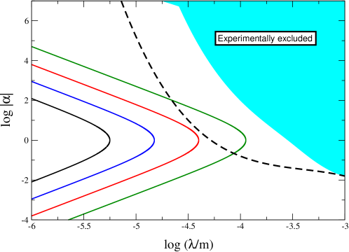
Figure 1: Comparison with table-top experiments. Solid curves are Eq. (5.3) with $d=3,4,5,6$, from top to bottom, respectively, and $M=1$ TeV. The shaded region is excluded from present experimental data, Ref. [2], while the dashed curve is the projected experimental sensitivity of Ref. [3].

In Fig. 1 we plot Eq. (5.3) for dimensions $d=3,4,5$ and $6$, solid curves from top to bottom, respectively, and $M=1$ TeV, and show, in the $(|\alpha|,\lambda)$ plane the present excluded region from table-top experiments, Ref. [2]. The dashed line represents the projected experimental sensitivity of Ref. [3]. The crossing of solid and dashed curves will impose some upper bounds on $\bar{M}$.

5.2 Collider phenomenology

We will assume in this subsection that $d\geq 2$ and $\bar{M}\stackrel{{\scriptstyle>}}{{{}_{\sim}}}M$, so that for the energies accessible at present and future high-energy collider we can approximate the Green function as one where the large number of KK modes behave like an “effective” resonance state, given by Eqs. (4.14), with mass $\mathcal{M}_{d}$ and width controlled by $\gamma_{d}$, Eq. (3.15). In the $\bar{M}\to 0$ limit (i.e. $s\ll\mathcal{M}_{d}^{2}$) one recovers the ADD (constant) result. However for values of $\bar{M}\stackrel{{\scriptstyle>}}{{{}_{\sim}}}M$ there will be important modifications of ADD collider phenomenology, both on KK graviton production and on virtual graviton mediated processes, that will be briefly analyzed in this section.

5.2.1 Production processes

As it was already emphasized in Ref. [1], processes with KK graviton production are an important signature of extra dimensions. They appear as missing-energy events where a particle (photon $\gamma$, quark $q$ or gluon $g$) is produced and no observable particle is balancing its transverse momentum.

Given the huge number of KK modes and, correspondingly, the smallness of their mass differences, we can replace the production sum of KK modes by a continuous integration, and write the differential cross-section for inclusive graviton production (i.e. $f\bar{f}\to\gamma X$, $q\bar{q}\to gX$, $qg\to qX$, $gg\to gX$) as

$$\frac{d\sigma}{dt}=\frac{1}{\pi}\int_{0}^{s}{\rm Im}\,\tilde{G}_{d}(m^{2})\frac{d\sigma_{m}}{dt}\,dm^{2}$$ (5.5)

where ${\displaystyle\frac{d\sigma_{m}}{d\,t}}$ is the differential cross-section for production of a single (canonically normalized) KK mode with mass $m$ and a coupling strength to matter $1/M_{Pl}^{2}$, and $\tilde{G}_{d}(m^{2})=M_{Pl}^{2}\ G_{d}(m^{2})$. The expression for ${\rm Im}\,\tilde{G}_{d}(m^{2})$ is given by

$${\rm Im}\,\tilde{G}_{d}(m^{2})=\frac{M_{Pl}^{2}}{\bar{M}^{2}}\left(1-\frac{\bar{M}^{2}}{M_{Pl}^{2}}\right)\,\frac{\gamma_{d}(m^{2})\,\mathcal{M}_{d}^{2}}{\left(\mathcal{M}_{d}^{2}-m^{2}\right)^{2}+\gamma_{d}^{2}(m^{2})\,m^{4}}\ .$$ (5.6)

From (5.6) we can see that for $m^{2}\ll\mathcal{M}_{d}^{2}$,

$${\rm Im}\,\tilde{G}_{d}(m^{2})\simeq\frac{\pi}{2}\,\frac{\Omega_{d}}{\pi^{d}}\,\frac{\left(m^{2}\right)^{d/2-1}M_{Pl}^{2}}{M^{2+d}}={\rm Im}\,\tilde{G}_{d}(m^{2})_{\rm ADD}\ .$$ (5.7)

In this way the KK modes which are much lighter than $\mathcal{M}_{d}$ couple to matter as in the ADD scenario. Therefore, if $\sqrt{s}<\mathcal{M}_{d}$, the differential cross section for the reaction $e^{+}e^{-}\to\gamma X$ is

$$\left.\frac{d\sigma}{d\cos\theta}\right|_{\sqrt{s}<\mathcal{M}_{d}}\simeq\frac{\alpha}{M^{2}}\left(\frac{\sqrt{s}}{M}\right)^{d}(1+\cos^{2}\theta)$$ (5.8)

where $\alpha$ is the electromagnetic constant and $\theta$ the scattering angle in the center-of-mass system.

On the other hand, for $m^{2}\gg\mathcal{M}_{d}^{2}$ the imaginary part of the Green function behaves as,

$${\rm Im}\,\tilde{G}_{d}(m^{2})\simeq\left(\frac{\mathcal{M}_{d}}{m}\right)^{4}\,{\rm Im}\,\tilde{G}_{d}(m^{2})_{\rm ADD}$$ (5.9)

and the corresponding KK modes couple to matter as $\sim\mathcal{M}^{4}_{d}/m^{4}$ times the ordinary Newton constant.

To estimate the integral in (5.5) we have found, for $\sqrt{s}\stackrel{{\scriptstyle>}}{{{}_{\sim}}}\mathcal{M}_{d}$, to a good accuracy,

$$\frac{d\sigma}{dt}\simeq\frac{M_{Pl}^{2}}{\bar{M}^{2}}\,\left(1-\frac{\bar{M}^{2}}{M_{Pl}^{2}}\right)\frac{d\sigma_{m}(\mathcal{M}^{2}_{d})}{dt}$$ (5.10)

where we have used the smallness of $\gamma_{d}$ and the property $\lim_{\varepsilon\to 0}\varepsilon/(x^{2}+\varepsilon^{2})=\pi\delta(x)$. In this way, the collective effect of all KK modes behaves as the production of a single sharp resonance of mass $\mathcal{M}_{d}$ and coupling $1/\bar{M}^{2}$. This signature is very distinct from ADD. For example, for $e^{+}e^{-}\to\gamma X$, and neglecting terms of $\mathcal{O}(\mathcal{M}_{d}^{2}/s)$, the differential cross section (5.10) can be written as [4]

$$\frac{d\sigma}{d\,\cos\theta}\simeq\frac{\pi\alpha}{\bar{M}^{2}}(1+\cos^{2}\theta)\ .$$ (5.11)

The modes with mass smaller and larger than $\mathcal{M}_{d}$ give a total contribution proportional to $1/M^{2}\left(\mathcal{M}_{d}/M\right)^{d}$ and $1/\bar{M}^{2}\left(s/M^{2}\right)^{d/2-1}\left(\mathcal{M}^{2}_{d}/s\right)$, respectively. These contributions are sub-dominant for $d>2$, while for $d=2$ can be at most of order of the contribution of the collective mode of mass $\mathcal{M}_{d}$, Eq. (5.11). In this way the present bounds from this process at LEP2 in ADD can be easily translated into the lower bound $\bar{M}\stackrel{{\scriptstyle>}}{{{}_{\sim}}}5$ TeV whenever $\mathcal{M}_{d}$ is kinematically accessible to this machine. If $\mathcal{M}_{d}$ is not energetically accessible, the bound on $\bar{M}$ disappears and it is replaced by a bound on $M$ similar to that obtained in the ADD case [4]. Of course much stronger bounds will be obtained from future accelerators.

5.2.2 Virtual exchange

The effective resonance of mass $\mathcal{M}_{d}$ can also contribute to physical processes by a single virtual exchange in the s-channel, along with the exchange of other standard model particles. It can contribute sizeably to the cross-sections if the center-of-mass energy $s$ is close to $\mathcal{M}_{d}$. In that case its contribution to the cross-sections is proportional to

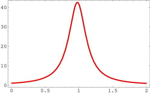
Figure 2: Plot of the function $f(s/\mathcal{M}_{d})$ for $d=3$ and $\mathcal{M}_{d}=0.1\,M$.

$$\frac{1}{\bar{M}^{4}\mathcal{M}_{d}^{4}}\,f(s/\mathcal{M}_{d}^{2})$$ (5.12)

with

$$f(s/\mathcal{M}_{d}^{2})=\mathcal{M}_{d}^{4}\ \frac{\left(s-\mathcal{M}_{d}^{2}+\gamma_{d}^{2}(s)\,s\right)^{2}+\gamma_{d}^{2}(s)\mathcal{M}_{d}^{4}}{\left[\left(\mathcal{M}_{d}^{2}-s\right)^{2}+\gamma_{d}^{2}(s)\,s^{2}\right]^{2}}\ .$$ (5.13)

At the resonance peak there is an enhancement, with respect to the (constant) ADD contribution, as

$$\left(\frac{\bar{M}^{2}}{M^{2}}\right)^{d-2}$$

while the distribution width

$$\sim\frac{\pi}{2}(d-2)\left(\frac{\mathcal{M}_{d}}{M}\right)^{d-2}$$

is essentially governed by the ratio $\mathcal{M}_{d}/M$. An example of the resonance distribution is given in Fig. 2, where the function $f(s/\mathcal{M}_{d})$ is plotted for the case $\mathcal{M}_{d}/M=0.1$ and $d=3$.

6 Conclusions

This paper deals with the effect of kinetic brane gravitational corrections on extra dimensional scenarios. These corrections can be induced by interactions of bulk gravitons with matter localized on the brane and their size is not protected by any four dimensional symmetry acting on the brane. To avoid the complication inherent to the tensor structure of the higher dimensional graviton we have worked out a prototype model with a simple scalar field propagating in the bulk of the extra dimensions. This work was partly motivated by the recent and interesting claim that for the case of two (or more) infinite size flat extra dimensions kinetic brane corrections trigger higher dimensional gravitons to be localized on the brane. Moreover, for finite size radius we also expect kinetic brane gravitational corrections to substantially modify the usual picture initially introduced by Arkani-Hamed, Dimopoulos and Dvali as an alternative solution to the hierarchy problem and, in particular, its implications on collider phenomenology and table-top gravitational experiments.

We have endowed the theory with both an IR and an UV regularization. The IR regularization is implemented by a $d$ dimensional torus with a common radius $R$. The infinite size can then be reached in the $R\to\infty$ limit. The UV regularization is provided by a physical UV cutoff $\Lambda$. Since the higher dimensional gravitational theory is an effective one, with a physical cutoff of the order of the higher dimensional Planck scale, $M$, the cutoff $\Lambda$ is restricted to be $\sim M$, or even less if the brane is fat, a possibility that, for simplicity, we are not considering.

For the case of infinite size extra dimensions, $R\to\infty$, were we allowed to take the $\Lambda\to\infty$ limit, we would recover the results of Refs. [5, 7]. However, as $\Lambda\stackrel{{\scriptstyle<}}{{{}_{\sim}}}M$, as we pointed out above, our results for infinite size extra dimensions do not lead to the existence of tensor gravity localized on the brane but, instead, lead in general to a massive graviton. To summarize, in the absence of a quantum field theory of gravity in higher dimensions, the existence of a physical UV cutoff prevents localization of tensor gravity on the brane in the presence of infinite size extra dimensions.

For the case of finite extra dimensions, kinetic brane gravitational corrections induce deep modifications on the ADD scenario. In particular the emergence of a “collective” state (made out of an “infinite” number of KK modes) with a mass $\mathcal{M}_{d}\sim M^{2}/\bar{M}$ and an effective coupling $G_{\rm eff}\sim 1/\bar{M}^{2}$, where $\bar{M}$ is the brane correction. For $\mathcal{M}_{d}\stackrel{{\scriptstyle<}}{{{}_{\sim}}}1/R$, this state can be detected in table-top gravitational experiments, while ADD collider phenomenology is deeply modified since KK gravitons become unobservable in high-energy colliders. On the other hand, for $1/R\stackrel{{\scriptstyle<}}{{{}_{\sim}}}\mathcal{M}_{d}\stackrel{{\scriptstyle<}}{{{}_{\sim}}}M$, table-top gravitational experiments are blind to the new state and so table-top gravitational phenomenology remains essentially unchanged. On the other hand the new resonance can be produced on-shell at high-energy colliders and then also modify the ADD phenomenology.

Appendix A Appendix

The integral (2.7) can be written in general for even and odd values of $d$.

• For $d$ odd:

  $$D_{d}(p,0)=\frac{1}{p^{2}R^{d}}\left\{1+\Omega_{d}\frac{R^{d}p^{d}}{\pi^{d}}\left[(-1)^{(d-1)/2}\left(\arctan\left(\frac{\Lambda}{p}\right)-\arctan\left(\frac{\pi}{Rp}\right)\right)\phantom{\frac{1^{1^{1}}}{1^{1^{1}}}}\right.\right.$$

  $$+\left.\left.\sum_{n=1}^{(d-1)/2}\frac{(-1)^{n-1}}{d-2n}\left(\left(\frac{\Lambda}{p}\right)^{d-2n}-\left(\frac{\pi}{Rp}\right)^{d-2n}\right)\right]\right\}\ .$$ (A.1)

• For $d$ even:

  $$D_{d}(p,0)=\frac{1}{p^{2}R^{d}}\left\{1+\Omega_{d}\frac{R^{d}p^{d}}{\pi^{d}}\left[(-1)^{d/2-1}\frac{1}{2}\left(\log\left(1+\frac{\Lambda^{2}}{p^{2}}\right)-\log\left(1+\frac{\pi^{2}}{R^{2}\,p^{2}}\right)\right)\phantom{\frac{1^{1^{1}}}{1^{1^{1}}}}\right.\right.$$

  $$+\left.\left.\sum_{n=1}^{d/2-1}\frac{(-1)^{n-1}}{d-2n}\left(\left(\frac{\Lambda}{p}\right)^{d-2n}-\left(\frac{\pi}{Rp}\right)^{d-2n}\right)\right]\right\}\ .$$ (A.2)

The analytic continuation of the function $D_{d}(p,0)$ into Minkowski space-time, $D_{d}(s)$, can be done by simply replacing in (A.1) and (A.2) $p\to-i\sqrt{s}$ and using the property, $\arctan(ix)=i\tanh^{-1}(x)$. The result can be written as:

• For $d$ odd:

  $$D_{d}(s)=\frac{1}{s\,R^{d}}\left\{-1+\Omega_{d}\frac{R^{d}}{\pi^{d}}\,s^{d/2}\left[i\,\frac{\pi}{2}-\tanh^{-1}\left(\frac{\sqrt{s}}{\Lambda}\right)+\tanh^{-1}\left(\frac{\pi}{R\,\sqrt{s}}\right)\phantom{\frac{1^{1^{1}}}{1^{1^{1}}}}\right.\right.$$

  $$+\left.\left.\sum_{n=1}^{(d-1)/2}\frac{1}{d-2n}\left(\left(\frac{\Lambda^{2}}{s}\right)^{\frac{d}{2}-n}-\left(\frac{\pi^{2}}{R^{2}\,s}\right)^{\frac{d}{2}-n}\right)\right]\right\}\ .$$ (A.3)

• For $d$ even:

  $$D_{d}(s)=\frac{1}{s\,R^{d}}\left\{-1+\Omega_{d}\frac{R^{d}}{\pi^{d}}\,s^{d/2}\left[i\,\frac{\pi}{2}+\frac{1}{2}\log\left(\frac{\Lambda^{2}}{s}-1\right)-\frac{1}{2}\log\left(1-\frac{\pi^{2}}{R^{2}\,s}\right)\phantom{\frac{1^{1^{1}}}{1^{1^{1}}}}\right.\right.$$

  $$+\left.\left.\sum_{n=1}^{\frac{d}{2}-1}\frac{1}{d-2n}\left(\left(\frac{\Lambda^{2}}{s}\right)^{\frac{d}{2}-n}-\left(\frac{\pi^{2}}{R^{2}\,s}\right)^{\frac{d}{2}-n}\right)\right]\right\}\ .$$ (A.4)

The imaginary part proportional to $\pi/2$ in Eqs. (A.3) and (A.4) come from the resonant production of a single KK mode with square mass equal to $s$ while the real part comes from the summation over non-resonant states.

Substituting the functions $D_{d}(p,0)$, as given by (A.1) or (A.2), and $D_{d}(s)$,as given by (A.3) or (A.4), into Eq. (2.3) provides the Green function $G_{d}(p,0)$, and its analytic continuation into the Minkowski space-time $G_{d}(s)$, for the bulk scalars.

References

- [1] N. Arkani-Hamed, S. Dimopoulos and G. Dvali, Phys. Lett. B429 (1998) 263; Phys. Rev. D59 (1999) 0860; I. Antoniadis, N. Arkani-Hamed, S. Dimopoulos and G. Dvali, Phys. Lett. B436 (1998) 257.
- [2] C.D. Hoyle et al., hep-ph/0011014.
- [3] J.C. Long, A.B. Churnside and J.C. Price, hep-ph/0009062.
- [4] G.F. Giudice, R. Rattazzi and J.D. Wells, Nucl. Phys. B544 (1999) 3; E.A. Mirabelli, M. Perelstein and M.E. Peskin, Phys. Rev. Lett. 82 (1999) 2236; T. Han, J.D. Lykken and R.-J. Zhang, Phys. Rev. D59 (1999) 105006; J. L. Hewett, Phys. Rev. Lett. 82 (1999) 4765.
- [5] G. Dvali, G. Gabadadze and M. Porrati, Phys. Lett. B485 (2000) 208.
- [6] H. Collins and B. Holdom, Phys. Rev. D62 (2000) 124008.
- [7] G. Dvali and G. Gabadadze, Phys. Rev. D63 (2001) 065007.
- [8] D. M. Capper, Nuovo Cim. A25 (1975) 29.
- [9] A. Zee, Phys. Rev. D23 (1981) 858; Phys. Rev. Lett. 48 (1982) 295.
- [10] S. L. Adler, Phys. Lett. B95 (1980) 241; Phys. Rev. Lett. 44 (1980) 1567; Rev. Mod. Phys. 54 (1982) 729; Erratum-ibid. 55 (1983) 837.
- [11] N. N. Khuri, Phys. Rev. D26 (1982) 2664; Phys. Rev. Lett. 49 (1982) 513.