Present and Future CP Measurements UK Phenomenology Workshop
September 2000 Durham

Abstract

We review theoretical and experimental results on CP violation summarizing the discussions in the working group on CP violation at the UK phenomenology workshop 2000 in Durham.

1 Introduction

In the standard $SU(2)\times U(1)$ gauge theory of Glashow, Salam and Weinberg predictions involving fermion masses and hadronic flavour changing weak transitions require a prior knowledge of the mass generation mechanism. The simplest method of giving mass to the fermions in the theory makes use of Yukawa interactions involving the doublet Higgs field. An as yet unconfirmed mechanism. These interactions give rise to the Cabibbo-Kobayashi-Maskawa (CKM) matrix: Quarks of different flavour are mixed in the charged weak currents by means of an unitary matrix $V$. However, both the electromagnetic current and the weak neutral current remain flavour diagonal. Second order weak processes such as mixing and CP–violation are even less secure theoretically, since they can be affected by both beyond the Standard Model virtual contributions, as well as new physics direct contributions. Our present understanding of CP–violation is based on the three-family Kobayashi-Maskawa model of quarks, some of whose charged-current couplings have phases. Over the past decade, new data have enabled considerable refinement of our knowledge of the parameters of this matrix $V$. Recent data based on the analysis of leptons with high center-of-mass momentum in B meson decays, indicate that the $b\to u$ transition matrix element is nonzero. The complex phase of this matrix element is very important for the successful description of CP–violation within the framework of the CKM matrix. Results of experiments searching for the difference between CP violating decays of kaons to pairs of neutral and charged pions have been presented by FNAL and CERN, which support our understanding of CP violation through the CKM matrix. The top quark enters into several constraints on CKM parameters through loop diagrams, so that such an analysis necessarily implies a favored range of top quark masses. Over the past decade or so, many methods have been proposed for obtaining the three interior angles of the unitarity triangle of the matrix $V$, $\alpha$, $\beta$ and $\gamma$. Presently these CP phases are being measured in a variety of experiments at B-factories, KEK-B, SLAC-B, HERA-B and will be measured at LHC-B and B-TeV. As always, the hope is that these measurements will reveal the presence of physics beyond the Standard Model.

The small visible branching ratio of B decays to CP eigenstates, $\cal O$(10^-5), requires a large number of B mesons to be produced in order to study CP violation in enough detail. The two complementary methods are $e^{+}e^{-}$ colliders tuned to the $\Upsilon$(4S) resonance or high energy hadron machines where the $b\overline{b}$ cross–section is large.

Current $e^{+}e^{-}$ colliders have achieved peak luminosities of $\sim 3\times 10^{33}$cm^-2s^-1 producing $b\overline{b}$ pairs at the rate of $\sim 1$ Hz, although raw data rates are considerably higher. The B mesons are produced in a coherent state and it is necessary to measure the time separation of both decay vertices to measure CP asymmetry in $B^{0}\overline{B^{0}}$ mixing. To this end both, both PEP-II and KEK use asymmetric beam energies to boost the distance between the decay vertices. Yet with typical separations of only $\sim 250\ \mu$m, the detectors used to resolve the vertices must still be as close as possible to the beam line to achieve suitable vertex accuracies of $\sim 50$-$100\ \mu$m. Symmetric energy machines can use the decays of charged B mesons for CP investigations. In all cases, the known initial beam energies, even in the presence of initial state radiation, is an important constraint, improving reconstructed B mass resolutions by an order of magnitude. The B_S system can be investigated by moving to the $\Upsilon(5S)$ resonance, although with a large reduction in cross–section.

The hadron colliders have the advantage of much higher production rates, ${\cal O}$($10^{4}$) Hz at the Tevatron and 10 times greater again at the LHC as well as producing both B and B_S mesons without then need for altering beam energies. As the centre of mass energy increases, the ratio of the $b\overline{b}$ to inelastic cross-section increases. The challenge is however to cope with the very high rates of background events and the large numbers of tracks in all events. These very high interaction rates require the use of sophisticated triggers operating at high rates. The beam crossing rate at the LHC for example is 40MHz while B decays that are interesting occur at a rate of a few Hz.

The accurate reconstruction of decay vertices and the ability to cleanly identify hadrons are major design requirements of both current and future detectors. Good vertex resolution requires the use of high precision vertex detectors very close to the beam pipe while the high particle fluxes place stringent requirements on the radiation hardness of the devices used. The large number of B hadrons produced means that, particularly at hadron machines, it becomes possible to make use of B decays with small cross sections where good differentiation between charged pions and kaons is required. High precision measurements in these final states will be the forte of the future experiments. This has prompted the development of high precision Cherenkov counters. The use of final states containing neutral particles requires the use of finely segmented calorimeters and will be particularly difficult at hadron colliders given the high backgrounds that will be encountered.

A complete review on the present status of CP measurements and their future prospects is beyond the scope of the present report. In this report we summarize the discussions in the working group on CP violation at the UK phenomenology workshop 2000 in Durham. In the following we give a short outline of the various topics which were addressed. In Section 2 we describe the measurements of $sin2\beta$  by the BaBar and the Belle experiment and discuss some prospects for the future. We also summarize CP violation measurements from $B$ decays observed at CDF during the last Tevatron run (Run-I). Prospects for measuring CP violation in the period between March 2001 and March 2003 (Run-II) at the upgraded CDF-II detector are also summarized. It is expected that the current generation of experiments will make the first observation of CP violation in the B system. We also concentrate on the anticipated performance of the next generation experiments, namely LHCb at CERN and BTeV at Fermilab, which will measure CP violating observables with extremely high precision, thereby thoroughly testing the Standard Model description of CP violation and searching for new physics beyond. In section 3 we focus on the influence of new physics on CKM phenomenology and on CP-violating observables. We also review various methods for determining the weak phase angle $\gamma$. Section 4 is devoted to the CP violation parameter $\epsilon^{\prime}/\epsilon$ within and beyond the SM. In Section 5 discussions on specific $B_{s}-$decays and on the width difference in the $B_{d}$-$\bar{B}_{d}$ system are included. In Section 6 we give an overview of the B-Physics trigger strategy for Run 2 at the Tevatron, with an emphasis on CP-Violation. Also the LHCb trigger strategy is reviewed. In addition a method to separate B events from continuum background in BaBar is presented. In Section 7 the phenomenological impact of the QCD-improved factorization approach is discussed while Section 8 deals with statistical issues relevant to heavy flavour physics including confidence level and the new technique due to Feldman an Cousins.

2 What ought we to be measuring?

2.1 The B A B AR  measurement of $\sin\!2\beta$  and its future prospects 

James Weatherall, Univ. Manchester (representing the B A B AR Collaboration)

2.1.1 Introduction

The B A B AR experiment consists of an asymmetric electron-positron collider operating at the $\Upsilon$(4S) resonance. More details on the detector can be found in [1]. The aim is to overconstrain the unitarity triangle by measuring its sides and angles. The analysis reviewed here measures $\sin\!2\beta$ by studying time-dependent $C\!P$ violating asymmetries in $B^{0}\rightarrow{J\mskip-3.0mu/\mskip-2.0mu\psi\mskip 2.0mu}K^{0}_{\scriptscriptstyle S}$ and $B^{0}\rightarrow\psi^{\prime}K^{0}_{\scriptscriptstyle S}$ decays.

2.1.2 Overview of the $\sin\!2\beta$ analysis

There are five main parts to measuring the $C\!P$ violating asymmetry:

• Selection of signal $C\!P$ events

• Measurement of the distance ${\rm\Delta}z$ between the two $B^{0}$ decay vertices along the $\Upsilon$(4S) boost axis

• Determination of the flavour of the tag-side B

• Measurement of dilution factors for the different tagging categories

• Extraction of $\sin\!2\beta$ via an unbinned maximum likelihood fit

Event Selection

The sample used for the analysis is 9.8 fb^-1 of data recorded between January and July 2000 of which 0.8 fb^-1 was recorded 40 MeV below the $\Upsilon$(4S) resonance. Particle identification uses mainly the CsI calorimeter for electrons, the Instrumented Flux Return for muons and the DIRC for kaons. Extra information is provided by dE/dx measured in the tracking system. The selection for the $C\!P$ events proceeds as follows. Pairs of electrons or muons coming from a common vertex are combined to form ${J\mskip-3.0mu/\mskip-2.0mu\psi\mskip 2.0mu}$ and $\psi^{\prime}$ candidates. The $\psi^{\prime}$ is also reconstructed from its decay into ${J\mskip-3.0mu/\mskip-2.0mu\psi\mskip 2.0mu}$ $\pi^{+}\pi^{-}$. The $K_{S}$ candidates are made from either a pair of charged tracks or a pair of $\pi^{0}$ candidates. In addition there are various event shape and topological cuts designed to reduce continuum and $B\overline{B}$ background. Full details of the selection can be found in [2]. The final event sample is shown in figure 1.

There are two other $B$ decay samples. One consists of fully reconstructed semileptonic ($B^{0}\to D^{*-}l^{+}\nu_{l}$) and hadronic ($B^{0}\to D^{(*)-}\pi^{+},D^{(*)-}\rho^{+},D^{(*)-}a_{1}^{+}$) decays as well as a control sample of $B^{+}\to\overline{D}^{(*)0}\pi^{+}$ events. The selection of this sample is described in [3] and [4]. The other is a charmonium control sample containing fully reconstructed neutral or charged $B$ candidates in two-body decay modes with a ${J\mskip-3.0mu/\mskip-2.0mu\psi\mskip 2.0mu}$ in the final state (e.g. $B^{+}\to{J\mskip-3.0mu/\mskip-2.0mu\psi\mskip 2.0mu}\ K^{+},B^{0}\to{J\mskip-3.0mu/\mskip-2.0mu\psi\mskip 2.0mu}\ K^{*0}(K^{*0}\to K^{+}\pi^{-})$).

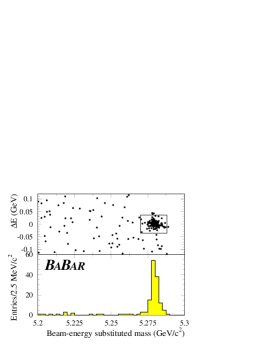
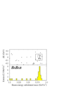
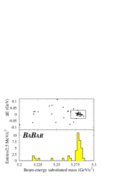
Figure 1: $C\!P$ signal event distributions for $J/\psi K_{S}(\pi^{+}\pi^{-})$ (left), $J/\psi K_{S}(\pi^{0}\pi^{0})$ (middle) and $\psi^{\prime}\ K_{S}(\pi^{+}\pi^{-})$ (right).

Measuring ${\rm\Delta}z$

The time-dependent decay rate for the $B_{C\!P}$ is given by

$$f_{\pm}(\,\Gamma,\,{\rm\Delta}m_{d},\,{\cal{D}}\sin{2\beta},\,t\,)={\frac{1}{4}}\,\Gamma\,{\rm e}^{-\Gamma\left|t\right|}\,\left[\,1\,\pm\,{\cal{D}}\sin{2\beta}\times\sin{{\rm\Delta}m_{d}\,t}\,\right]$$ (1)

where the + or - sign indicates whether the $B_{tag}$ was tagged as a $B^{0}$ or ${\kern 1.99997pt\overline{\kern-1.99997ptB}}^{0}$ respectively. The dilution factor $\cal{D}$ is given by ${\cal D}=1-2w$, where $w$ is the mistag fraction (the probability that the $B_{tag}$ is identified incorrectly). To account for finite detector resolution, the time distribution must be convoluted with a resolution function:

$${\cal{R}}({\rm\Delta}z;\hat{a}\,) = \sum^{2}_{i=1}\,\frac{f_{i}}{\sigma_{i}\sqrt{2\pi}}\,{\rm exp}\left(-({\rm\Delta}z-\delta_{i})^{2}/2{\sigma_{i}}^{2}\right)\ \ \ ,$$ (2)

which is just the sum of two Gaussians where the $f_{i}$, $\delta_{i}$ and $\sigma_{i}$ are the normalizations, biases and widths of the distributions. In practice two scale factors ${\cal S}_{1}$ and ${\cal S}_{2}$ are introduced such that $\sigma_{i}={\cal S}_{i}\times\sigma_{\Delta t}$ where $\sigma_{\Delta t}$ is an event-by-event calculated error on $\Delta t$. They take account of underestimating the uncertainty on $\Delta t$ due to effects such as hard scattering and possible underestimation of the amount of material traversed by the particles. The resolution function parameters are obtained from a maximum likelihood fit to the hadronic $B^{0}$ sample and are shown in table 1. The $f_{w}$ parameter represents the width of a third Gaussian component, included to accommodate a small ($\sim$1%) fraction of events which have very large values of $\Delta z$, mostly caused by vertex reconstruction problems. This Gaussian is unbiased with a fixed width of 8 ps. Further details can be found in [3].

Parameter		Value
$\delta_{1}$	(ps)	$-0.20\pm 0.06$	from fit
${\cal S}_{1}$		$1.33\pm 0.14$	from fit
$f_{w}$	(%)	$1.6\pm 0.6$	from fit
$f_{1}$	(%)	$75$	fixed
$\delta_{2}$	(ps)	$0$	fixed
${\cal S}_{2}$		$2.1$	fixed

Table 1: Resolution function parameters. Those, labeled ’from fit’ are measured from data and those marked ’fixed’ are determined from Monte Carlo.

B flavour tagging

Each event with a $C\!P$ candidate is assigned a $B^{0}$ or ${\kern 1.99997pt\overline{\kern-1.99997ptB}}^{0}$ tag if it satisfies the criteria for one of the several tagging categories. The figure of merit for each tagging category is the effective tagging efficiency $Q_{i}=\epsilon_{i}(1-2w_{i})^{2}$ where $\epsilon_{i}$ is the fraction of events assigned to category $i$ and $w_{i}$ is the probability of mis-tagging an event in this category. The statistical error on $\sin\!2\beta$ is proportional to $1/\sqrt{Q}$ where $Q=\sum_{i}Q_{i}$. There are five tagging categories: Electron, Muon, Kaon, NT1 and NT2.

The first three require the presence of a fast lepton and/or one or more charged kaons in the event and depend on the correlation between the charge of a primary lepton or kaon and the flavour of the $b$ quark. If an event is not assigned to either the Electron or Muon categories, it is assigned to the Kaon category if the sum of the charges of all the identified kaons in the event is different from zero. If both lepton and kaon tags are available but inconsistent the event is rejected from both categories.

NT1 and NT2 are categories from a neural network algorithm, this approach being motivated by the potential flavour-tagging power carried by non-identified leptons and kaons, correlations between leptons and kaons and more generally the momentum spectrum of charged particles from $B$ meson decays. The output of the neural network tagger $x_{NT}$ can be mapped onto the interval [-1,1] with $x_{NT}<0$ representing a $B^{0}$ tag and $x_{NT}>0$ a ${\kern 1.99997pt\overline{\kern-1.99997ptB}}^{0}$ tag. Events with $|x_{NT}|>0.5$ are classified in the NT1 category and events with $0.2<|x_{NT}|<0.5$ in the NT2 category. Events with $|x_{NT}|<0.2$ are excluded from the final analysis sample.

Measurement of tagging performance

The effective tagging efficiencies and mistag fractions for all the categories are measured from data using a maximum likelihood fit to the time distributions of the $B^{0}$ hadronic event sample. The procedure uses events which have one $B$ fully reconstructed in a flavour eigenstate mode. The tagging algorithms are then applied to the rest of the event, which represents the potential $B_{tag}$. Events are classified as mixed or unmixed depending on whether the $B_{tag}$ is tagged with the same or opposite flavour as the $B_{CP}$. One can express the time-integrated fraction of mixed events $\chi$ as a function of the $B^{0}{\kern 1.99997pt\overline{\kern-1.99997ptB}}^{0}$ mixing probability, $\chi=\chi_{d}+(1-2\chi_{d})w$ where $\chi_{d}=\frac{1}{2}x^{2}_{d}/(1+x^{2}_{d})$, with $x_{d}=\Delta m_{d}/\Gamma$. Thus an experimental value of the mistag fraction $w$ can be deduced from the data.

A more accurate estimate of $w$ comes from a time-dependent analysis of the fraction of mixed events. The mixing probability is smallest at low $\Delta t$ so that this region is governed by the mistag fraction. Figure 2 shows the fraction of mixed events versus $\Delta t$. The resultant tagging performances are shown in table 2.

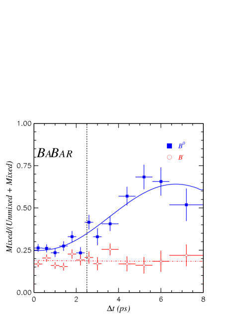
Figure 2: The fraction of mixed events as a function of $|\Delta t|$ for data events in the hadronic sample for neutral $B$ mesons (full squares) and charged $B$ mesons (open circles). The dot-dashed line at $t_{cut}=2.5$ ps indicates the bin boundary for the time-integrated single-bin method.

Tagging category	$\epsilon$ (%)	$w$ (%)	$Q$ (%)
Lepton	$11.2\pm 0.5$	$9.6\pm 1.7\pm 1.3$	$7.3\pm 0.3$
Kaon	$36.7\pm 0.9$	$19.7\pm 1.3\pm 1.1$	$13.5\pm 0.3$
NT1	$11.7\pm 0.5$	$16.7\pm 2.2\pm 2.0$	$5.2\pm 0.2$
NT2	$16.6\pm 0.6$	$33.1\pm 2.1\pm 2.1$	$1.9\pm 0.1$
all	$76.7\pm 0.5$		$27.9\pm 0.5$

Table 2: Tagging performance as measured from data.

Extracting $\sin\!2\beta$

A blind analysis technique was adopted for the extraction of $\sin\!2\beta$ to eliminate possible experimenter bias. The technique hides both the result of the likelihood fit and the visual $C\!P$ asymmetry in the $\Delta t$ distribution. This method allows systematic studies to be performed while keeping the numerical value of $\sin\!2\beta$ hidden.

Possible systematic effects due to uncertainty in the input parameters to the fit, incomplete knowledge of the time resolution function, uncertainties in the mistag fractions and possible limitations in the analysis procedure were all studied. Details can be found in [2]. The systematic errors are summarized in table 3.

Source of uncertainty	Uncertainty on $\sin\!2\beta$
uncertainty on $\tau^{0}_{B}$	0.002
uncertainty on $\Delta m_{d}$	0.015
uncertainty on $\Delta z$ resolution for $C\!P$ sample	0.019
uncertainty on time-resolution bias for $C\!P$ sample	0.047
uncertainty on measurement of mistag fractions	0.053
different mistag fractions for $C\!P$ and non-$C\!P$ samples	0.050
different mistag fractions for $B^{0}$ and ${\kern 1.99997pt\overline{\kern-1.99997ptB}}^{0}$	0.005
background in $C\!P$ sample	0.015
total systematic error	0.091

Table 3: Summary of systematic uncertainties. The different contributions are added in quadrature.

Results and checks

The maximum likelihood fit for $\sin\!2\beta$, using the full tagged sample of 120 $B^{0}\rightarrow{J\mskip-3.0mu/\mskip-2.0mu\psi\mskip 2.0mu}K^{0}_{\scriptscriptstyle S}$ and $B^{0}\rightarrow\psi^{\prime}K^{0}_{\scriptscriptstyle S}$ events yields:

$$\sin\!2\beta\ =0.12\pm 0.37\,(stat)\pm 0.09\,(syst)\ (preliminary).$$ (3)

The log likelihood is shown as a function of $\sin\!2\beta$ in figure 3. The raw asymmetry as a function of $\Delta t$ is shown in figure 4

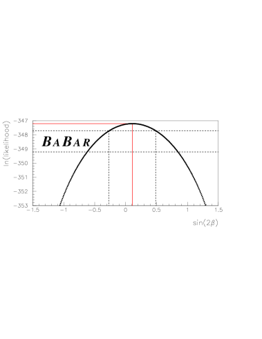
Figure 3: Variation of the log likelihood as a function of $\sin\!2\beta$. The two horizontal dashed lines indicate changes in the log-likelihood corresponding to one and two statistical standard deviations.

Figure 4: The raw $B^{0}-{\kern 1.99997pt\overline{\kern-1.99997ptB}}^{0}$ asymmetry $(N_{B^{0}}-N_{{\kern 1.39998pt\overline{\kern-1.39998ptB}}^{0}})/(N_{B^{0}}+N_{{\kern 1.39998pt\overline{\kern-1.39998ptB}}^{0}})$. The time-dependent asymmetry is represented by a solid curve for the central value of $\sin\!2\beta$, and by two dotted curves for the values at plus and minus one statistical standard deviation from the central value. The curves are not centered at (0,0) because the $C\!P$ sample contains an unequal number of $B^{0}$ and ${\kern 1.99997pt\overline{\kern-1.99997ptB}}^{0}$ events (70 $B^{0}$ versus 50 ${\kern 1.99997pt\overline{\kern-1.99997ptB}}^{0}$). The $\chi^{2}$ between the binned asymmetry and the result of the maximum likelihood fit is 9.2 for 7 degrees of freedom.

The probability of obtaining a statistical uncertainty of 0.37 is estimated by generating a large number of toy Monte Carlo experiments with the same number of tagged $C\!P$ events as in the data sample. The errors are distributed around 0.32 with a standard deviation of 0.03, meaning that the probability of obtaining a larger statistical error that the one observed is 5%. From a large number of full Monte Carlo simulated experiments, we estimate that the probability of finding a lower value of the likelihood than the one observed is 20%.

Several cross-checks are performed to validate the main analysis. The charmonium and fully-reconstructed hadronic control samples are composed of events that should exhibit no time-dependent asymmetry. These events are fitted in the same way as the signal $C\!P$ events to extract an “apparent $C\!P$ asymmetry”. The results are shown in table 4.

Sample	Apparent $C\!P$ asymmetry
Hadronic charged $B$ decays	$0.03\pm 0.07$
Hadronic neutral $B$ decays	$-0.01\pm 0.08$
$J/\psi K^{+}$	$0.13\pm 0.14$
$J/\psi K^{*0}(K^{*0}\to K^{+}\pi^{-})$	$0.49\pm 0.26$

Table 4: Summary of systematic uncertainties. The different contributions are added in quadrature.

Constraints on the unitarity triangle

The Unitarity Triangle in the ($\overline{\rho},\overline{\eta}$) plane is shown in figure 5. The two solutions corresponding to the measured central value are shown as straight lines. The cross-hatched regions correspond to one and two times the one-standard-deviation experimental uncertainty. The ellipses represent regions allowed by all other measurements that constrain the triangle. They are shown for a variety of choices of theoretical parameters. More details can be found in [5].

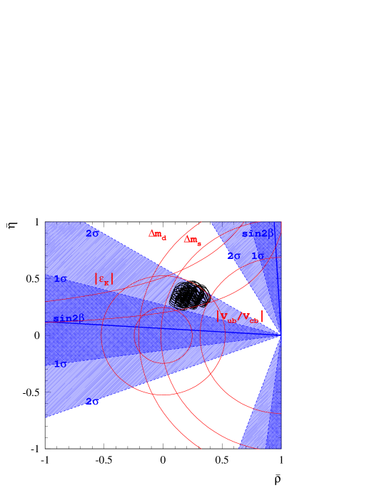
Figure 5: Present constraints on the position of the apex of the Unitarity Triangle with the B A B AR result indicated by the cross-hatched regions.

2.1.3 Future prospects

The preceding pages describe only a preliminary measurement of $\sin\!2\beta$ by the B A B AR experiment. More data will allow extra channels to be included in the final fit as well as providing more events for the currently used decay modes. The new channels will bring extra experimental and theoretical challenges with them. Such present and future issues are discussed in the sections that follow.

Available modes

The B decay modes that have been used to measure $\sin\!2\beta$ up to now are clean in that they are vector-scalar, $b\to ccs$ transitions which have no significant pollution from penguin diagrams. The next step is to add vector-vector modes such as $B^{0}\to J/\psi K^{*}$. These modes require an angular analysis of the vector meson decay products, due to the different partial waves and therefore admixture of $C\!P$ odd and $C\!P$ even that is present in the final state. Such an angular analysis has already yielded preliminary results for the $J/\psi K^{*}$ modes. Once one has measured the polarizations in these modes, they are as clean, theoretically, as the vector-scalar modes. Another obvious addition is $B^{0}\to J/\psi K_{L}$ decays where the challenge here is to understand the background well enough to make the channel feasible. Work is ongoing in this area.

A different kind of difficulty is presented by channels with a significant degree of penguin contamination, such as $b\to ccd$ scalar-scalar modes (e.g. $B^{0}\to D^{+}D^{-}$). Here the fit must take into account the fact that the true value of $\sin\!2\beta$ is shifted by an amount proportional to the ratio of tree to penguin contributions. This ratio is model dependent and subject to large theoretical uncertainties.

Finally, modes such as $B^{0}\to D^{*}D^{*}$ and $B\to J/\psi\rho^{0}$ which are vector-vector, $b\to ccd$ transitions face the theoretical challenges of the penguin contaminated modes described above, as well as requiring an angular analysis to solve the vector-vector $C\!P$ admixture problem.

Experimental considerations

There are also experimental analysis issues which need to be resolved or studied in greater depth in the future. The tagging algorithms that B A B AR uses should be developed and extended to include extra tagging categories such as the using the soft pion from $D^{*}$ decays and incorporating leptons at an intermediate momentum (i.e. from a cascade). It would be useful to take account of correlations within an event, such as when two different tagging categories report an answer. This can give more information about the event if the correlations are well understood. There is also an open question when it comes to measuring the tagging performance from the hadronic or semileptonic $B$ decay samples. One then needs to be absolutely sure that using exactly the same numbers for the $C\!P$ signal event sample is a valid thing to do.

The measurement of $\Delta z$ is another crucial part of the analysis and it is important that the errors and biases to this distribution are understood. The distribution tends to be biased by the decays of particles which fly significantly from the original $B$ decay vertex, such as $D^{0}$s. These can be rejected by looking explicitly for cascade decays. The parameterization of the resolution function incorporates detector effects such as misalignments and electronics readout effects. All contributions to the width should be studied in order to fully understand the error on $\Delta z$.

Backgrounds to the various $C\!P$ modes can also be a problem. The channels vary in terms of how much background they experience and this background can be particularly dangerous if it has a significant structure in $\Delta z$. For charmonium channels, much of the background comes from events containing a real $J/\psi$. In that case, one needs to study exactly which modes contribute and what their shape is in the final distributions (if they cannot be removed otherwise). Non-resonant backgrounds to vector-vector modes such as the $J/\psi K^{0}\pi^{0}$ contribution to $J/\psi K^{*0}(K^{*0}\to K^{0}\pi^{0})$ are in principle dangerous since they can have $C\!P$ violating properties but no angular structure. However, the branching ratios for these non-resonant modes are typically poorly known and consistent with zero making it difficult to simulate them in the correct proportions.

Study of statistical error

It seems anomalous that both B A B AR and Belle record higher statistical errors than one would expect. The fitting procedure is, and continues to be a vigorously studied part of the analysis as we need to be certain that the likelihood function is of exactly the correct form for the final fit.

2.1.4 Conclusions

A preliminary measurement of $\sin\!2\beta$ by B A B AR has been presented. The errors on the final result make it difficult to express its significance in terms of constraints on the Unitarity Triangle. However, results based on a much larger data sample ($\sim$20 fb^-1) will soon be available. Combined with a better understanding of systematic effects, this should make the next measurement of $\sin\!2\beta$ even more interesting than the current one. It is also expected that other $C\!P$ modes will soon be available for analysis including $B^{0}\to J/\psi K^{*0}(K^{*0}\to K_{S}\pi^{0})$ and $B^{0}\to J/\psi K_{L}$. The larger data sample with additional $C\!P$ modes should yield a value of $\sin\!2\beta$ for which the statistical and systematic errors are about one-half of their current values.

References

2.2 The first results from Belle

Yoshihito Iwasaki, KEK-IPNS (representing the Belle Collaboration)

2.2.1 Introduction

Observation of $C\!P$  violation in the $B$ meson system is one of the most exciting physics targets at a $B$ factory experiment. In the standard model, $C\!P$  violation is a natural consequence of the complex phase of quark mixing in the weak interaction as described by the Kobayashi-Maskawa matrix[1] . This phase can be detected in physics processes where amplitudes with different KM phase interfere.

In the decay of the neutral $B$ meson to a $C\!P$  eigenstate, at least two amplitudes ($A(B^{0}\to f_{CP})$ and $A(B^{0}\to\bar{B}^{0}\to f_{CP})$) exist due to $B^{0}$-$\bar{B}^{0}$ mixing. These amplitudes interfere. The time dependent $C\!P$asymmetry in the decay rate of $B^{0}$ and $\bar{B}^{0}$, $a_{CP}(t)$, can be written as[2]

$$a_{CP}(t) = {{\Gamma(B^{0}(t)\to f_{CP})-\Gamma(\overline{B}^{0}(t)\to f_{CP})}\over{\Gamma(B^{0}(t)\to f_{CP})+\Gamma(\overline{B}^{0}(t)\to f_{CP})}}$$ (4)

$$= \eta_{CP}\sin 2\phi_{1}\cdot\sin(\Delta mt),$$ (5)

where $t$ is the proper decay time of the $B$, $\eta_{CP}$ is the $C\!P$  eigenvalue of the final state $f_{CP}$, $\Delta m$ is the mass difference between the two $B^{0}$ mass eigenstates, and $\phi_{1}$ (also known as $\beta$) is one of the three angles of the CKM unitarity triangle formed by the $d$ and $b$ quark,

$$\phi_{1}\equiv\pi-\arg(\frac{-V^{*}_{tb}V_{td}}{-V^{*}_{cb}V_{cd}}).$$ (6)

In a $B$ factory experiment, a $B\bar{B}$ pair is created from $\Upsilon_{4S}$ decay in a coherent quantum state. At the decay of one $B$, the other $B$ oscillates starting with the opposite flavour of the $B$. Experimentally we measure $\Delta t=t_{CP}-t_{tag}$ instead of $t$, where $t_{CP}$ is the decay time of the neutral $B$ meson decaying to a $C\!P$  eigenstate($B_{CP}$), and $t_{tag}$ is the decay time of the other $B$($B_{tag}$). The flavour of $B_{tag}$ specifies the flavour of $B_{CP}$ at the start of the $B^{0}$-$\bar{B}^{0}$ mixing. To extract $\sin 2\phi_{1}\;$, we measure the proper time difference distributions instead of $a_{CP}(t)$ :

$$\frac{dN}{dt}=\frac{1}{2\tau_{B^{0}}}\exp(-\frac{|\Delta t|}{\tau_{B^{0}}})(1-\eta_{CP}\sin 2\phi_{1}\sin(\Delta m_{d}\Delta t))$$ (7)

2.2.2 KEKB accelerator and Belle detector

KEKB is an asymmetric energy $e^{+}e^{-}$ collider that produces a boosted $\Upsilon_{4S}$ in the laboratory frame. The beam energies of $e^{+}$ and $e^{-}$ are $3.5$ and $8.0$ GeV, respectively. The boost factor of the $\Upsilon_{4S}$ is $0.425$. The beam size at the interaction point is $2\mu m$ and $100\mu m$ in the vertical and horizontal direction, respectively.

The Belle detector is located at the interaction point of KEKB in the Tsukuba experimental hall. Construction was started in 1994 and completed in 1998. Belle is a general-purpose detector with a Silicon Vertex Detector (SVD), a Central Drift Chamber (CDC), an Aerogel Cherenkov Counter (ACC), a Time Of Flight scintillation counter (TOF), an Electro-magnetic Calorimeter (ECL), a solenoid magnet, and a $K_{L}$ muon catcher (KLM). Because the beam energies are asymmetric, the detector shape is also asymmetric in the beam direction in order to cover a large solid angle in the $\Upsilon_{4S}$ rest frame.

Charged tracks are reconstructed from CDC and SVD hits as the particle spirals in the solenoidal 1.5 Tesla magnetic field. The transverse momentum resolution is $\sigma_{p_{t}}/p_{t}=0.0019p_{t}\oplus 0.0034$. The impact parameter resolution in the plane perpendicular to the beam axis is $\sigma_{r\phi}=21\oplus\frac{69}{p\beta\sin^{3/2}\theta}$ $\mu$m where $p$ is the momentum in GeV and $\beta$ is the velocity. The impact parameter resolution along the beam direction is $\sigma_{z}=39\oplus\frac{51}{p\beta\sin^{5/2}\theta}$ $\mu$m.

Photons are reconstructed from the energy deposited in the ECL with a resolution of $\sigma_{E}/E=0.013\oplus 0.0007/E\oplus 0.008/E^{1/4}$, where $E$ is the measured energy in GeV. Kaons are identified using probabilities calculated from $dE/dx$ measured by CDC, TOF, and hits in ACC. The time resolution of the TOF is $95$ ps. The refractive index used by the ACC is chosen to provide good $\pi$/K separation for $1.5<p<3.5$ GeV. The efficiency is $\sim 80$% and the fake rate is $\sim 10$% for momentum up to $3.5$ GeV. Electron identification is done using $dE/dx$, ACC hits, and energy deposited in the ECL. The efficiency is above 90% for $p>1.0$ GeV. The fake rate is below $0.5$%. Muon identification is done with hits in the KLM. The efficiency is above $90$% and the fake rate is below $2$%.

2.2.3 Event selection of $C\!P$  eigenstates

The $C\!P$  eigenstates we search for are charmonium plus $K^{0}$ as listed in table 5. All decay modes include $b\to c\bar{c}s$ transitions except for $B^{0}\to J/\psi(l^{+}l^{-})+\pi^{0}$, which is a $b\to c\bar{c}d$ transition.

Candidate $J/\psi$ mesons are formed from pairs of oppositely charged tracks where at least one track is positively identified as a lepton ($\mu$ or $e$) and the other is consistent with a lepton. For the $J/\psi\to e^{+}e^{-}$ channel we also include $\gamma$’s within $0.05$ radians of the electron direction to recover events with initial state radiation from the $e$. We require the invariant mass of a lepton pair to be $-0.006$ GeV $<M_{\mu^{+}\mu^{-}}-M_{J/\psi}<0.036$ GeV and $-0.150$ GeV $<M_{e^{+}e^{-}}-M_{J/\psi}<0.036$ GeV for $\mu^{+}\mu^{-}$ and $e^{+}e^{-}$ pairs, respectively. For $\psi^{\prime}\to l^{+}l^{-}$ we require the invariant mass of the lepton pair to be $-60$ MeV $<M_{\mu^{+}\mu^{-}}-M_{\psi^{\prime}}<36$ MeV and $-150$ MeV $<M_{e^{+}e^{-}}-M_{\psi^{\prime}}<36$ MeV for $\mu^{+}\mu^{-}$ and $e^{+}e^{-}$ pairs, respectively. For $\psi^{\prime}\to J/\psi\pi^{+}\pi^{-}$ we combine a $J/\psi$ candidate and a $\pi^{+}\pi^{-}$, where the invariant mass of the pion pair is required to be greater than $400$ MeV. We require the mass difference of $\psi^{\prime}(l^{+}l^{-}\pi^{+}\pi^{-})$ and $J/\psi$ to be between $0.58$ GeV and $0.60$ GeV. For $\chi_{c1}\to J/\psi\gamma$, we combine a $\gamma$ and $J/\psi$ where the $\gamma$ is not consistent with forming $\pi^{0}$ when combined with any other $\gamma$.

For $K_{S}\to\pi^{+}\pi^{-}$ we select a pair of oppositely charged tracks where the closest distance of two tracks in the $z$ coordinate is consistent with zero. The invariant mass of the candidate is required to be within $\pm 3\sigma$ ($\pm 16$ MeV) of the $K_{S}$ mass peak. For $K_{S}\to\pi^{0}\pi^{0}$ we use pairs of $\pi^{0}$’s where $\pi^{0}$ is reconstructed from two $\gamma$’s. We require the invariant mass of $K_{S}$ and $\pi^{0}$ to be within the range $0.3$ GeV to $1.0$ GeV and $118$ MeV to $150$ MeV, respectively.

For $J/\psi\pi^{0}$ we select a high momentum $\pi^{0}$ reconstructed by two $\gamma$’s where the energy of each $\gamma$ is required to be greater than $100$ MeV. The invariant mass requirement is identical to the $\pi^{0}$ requirements in $K_{S}$ reconstruction.

Decay mode	$C\!P$	$\Delta E$ (MeV)	$N$	$N_{bg}$	$N_{tagged}$
$B^{0}\to J/\psi(l^{+}l^{-})+K_{S}(\pi^{+}\pi^{-})$	$-1$	$\pm 40$	70	3.4	40
$B^{0}\to J/\psi(l^{+}l^{-})+K_{S}(\pi^{0}\pi^{0})$	$-1$	$\pm 100$	4	0.3	4
$B^{0}\to\psi^{\prime}(l^{+}l^{-})+K_{S}(\pi^{+}\pi^{-})$	$-1$	$\pm 40$	5	0.2	2
$B^{0}\to\psi^{\prime}(J/\psi(l^{+}l^{-})\pi^{+}\pi^{-})+K_{S}(\pi^{+}\pi^{-})$	$-1$	$\pm 40$	8	0.6	3
$B^{0}\to\chi_{C1}(J/\psi(l^{+}l^{-})\gamma)+K_{S}(\pi^{+}\pi^{-})$	$-1$	${}^{+30}_{-40}$	5	0.75	3
$B^{0}\to J/\psi(l^{+}l^{-})+K_{L}$	$+1$	-	102	56	42
$B^{0}\to J/\psi(l^{+}l^{-})+\pi^{0}$	$+1$	${}^{+50}_{-100}$	10	1	4

Table 5: The decay modes of $B^{0}$ going to $C\!P$  eigenstate. $l$ represents $e$ or $\mu$.

For selection of $B$ candidates in all modes except for $B\to J/\psi K_{L}$, we use the energy difference $\Delta E\equiv E_{B}-E_{cm}/2$ and the beam-constrained mass $M_{beam}\equiv\sqrt{(E_{cm}/2)^{2}-P_{B}^{2}}$. In figure 6, the scatter plot of $\Delta E$ versus $M_{beam}$ is shown for $B\to J/\psi K_{S}(\pi^{+}\pi^{-})$. We define the signal region to be $|\Delta E|<40$ MeV and $|M_{beam}-\left\langle M_{beam}\right\rangle|<10$ MeV where $\left\langle M_{beam}\right\rangle$ is the mean of the observed $M_{beam}$. The signal region in $\Delta E$ is varied depending on the decay mode (see table 5). However, the signal region in $M_{beam}$ is the same as that for $B\to J/\psi K_{S}$ because the error on $M_{beam}$ is dominated by the beam energy spread.

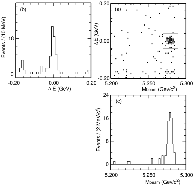
Figure 6: (a) The scatter plot of $\Delta E$ versus $M_{beam}$ for $B^{0}\to J/\psi K_{S}$ candidates. (b) The projection in $\Delta E$ with the cut $|M_{beam}-M_{B^{0}}|<0.01$ GeV. (c) The projection in $M_{beam}$ with the cut $|\Delta E|<0.04$.

For $B\to J/\psi K_{L}$ we use tighter cuts for $J/\psi$ reconstruction by requiring positive identification for both leptons and the momentum of the $J/\psi$($P^{*}_{J/\psi}$) in the CMS frame to be $1.42<P^{*}_{J/\psi}<2.00$ GeV. We reconstruct the momentum of the $K_{L}$ from the momentum of the $J/\psi$ with the assumption of a two body decay $B\to J/\psi K_{L}$. We also require associated KLM hits in the direction of the $K_{L}$ momentum. To select signal events we require the momentum of the $B$ in the CMS, $P^{*}_{B}$, to be in the range $200$ MeV $\leq P_{B}\leq 450$ MeV. A true candidate should peak around $340$ MeV corresponding to the initial momentum of the $B$ from the $\Upsilon_{4S}$. In figure 7, the $P^{*}_{B}$ distribution for $J/\psi K_{L}$ candidates is shown with the expectation obtained by a full MC simulation study. In the signal region, we have 102 $J/\psi K_{L}$ candidates where we expect $8$ background events from $B\to J/\psi K_{L}\pi^{0}$ (a mixture of $C\!P+1$ and $C\!P-1$) and $48$ background events from other sources.

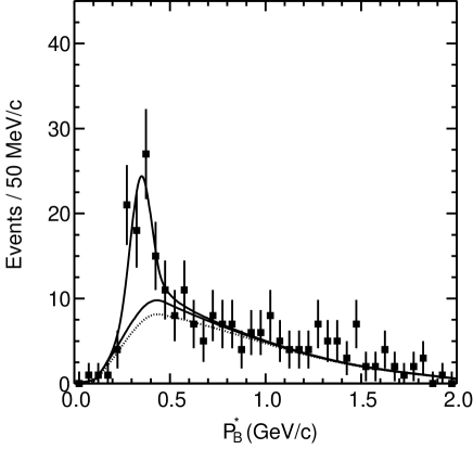
Figure 7: The $P^{*}_{B}$ distribution for $B\to J/\psi K_{L}$ candidates. The upper solid line is the fit of a sum of the signal and background expected from MC simulation studies. The lower solid line is the total background. The dotted line is the background component from sources other than $B\to J/\psi K_{L}\pi^{0}$.

2.2.4 Flavour tagging

To determine the flavour ($B^{0}$ or $\bar{B}^{0}$) of the $B_{CP}$ candidates, we partially reconstruct the other $B_{tag}$ in the event. The flavour of the $B_{CP}$ should be opposite to that of the $B_{tag}$ at the decay time of the $B_{tag}$($\Delta t=0$). We apply four methods sequentially.

1. the charge of a high momentum lepton ($P^{*}_{l}>1.1$ GeV) : This tags the flavour via its primary leptonic decay. We assign $B_{CP}=B^{0}(\bar{B}^{0})$ if the charge is positive(negative).

2. sum of the charge for positively identified kaons : This relies on $s$ quark pop-up in cascade decays. We assign $B_{CP}=B^{0}(\bar{B}^{0})$ if the sum of the charge is positive(negative).

3. the charge of a medium momentum lepton : This is similar to method (1) but for the case where there is large missing momentum in the CMS($P^{*}_{miss}$). We require the lepton momentum to be in the range $0.6<P^{*}_{l}<1.1$ GeV and the missing momentum in the CMS should satisfy $P^{*}_{l}+P^{*}_{miss}\geq 2.0$ GeV. The flavour assignment is identical to method (1).

4. the charge of slow pion : This tags the flavour of $D^{*}$ coming from $B_{tag}$. We require the momentum of the slow $\pi$ to be less than $200$ MeV. We assign $B_{CP}=B^{0}(\bar{B}^{0})$ if the pion charge is negative (positive).

The flavour tagging efficiency, $\epsilon$, and the wrong tag fraction, $\omega$, are measured from data with self-tagging decay modes. We exclusively reconstruct $B^{0}\to D^{(*)-}l^{+}\nu$, and apply the flavour tagging methods for the rest of the event. Because of $B^{0}$-$\bar{B}^{0}$ mixing, the probability to find the opposite or same flavour for the exclusively reconstructed $B$ and the result of the flavour tagging is

$$P_{opposite}(\Delta t) \propto 1+(1-2\omega)\cos(\Delta m_{d}\Delta t)$$ (8)

$$P_{same}(\Delta t) \propto 1-(1-2\omega)\cos(\Delta m_{d}\Delta t).$$ (9)

Then, $\omega$ can be extracted from the amplitude of the $B^{0}$-$\bar{B}^{0}$ mixing

$$A\equiv\frac{P_{opposite}-P_{same}}{P_{opposite}+P_{same}}=(1-2\omega)\cos(\Delta m_{d}\Delta t).$$ (10)

The vertex position of the $D^{(*)-}l^{+}\nu$ is determined by requiring the $l$ and $D^{(*)}$ to form a common vertex. The determination of the vertex position of the $B_{tag}$ is described in the next section. $\Delta t$ is calculated from the difference of the two vertices in the $z$ direction. We perform an unbinned maximum likelihood fit to the amplitude of the $B^{0}$-$\bar{B}^{0}$ mixing to obtain $\omega$ with $m_{d}$ allowed to be free. In table 6, $\epsilon$ and $\omega$ are summarized. We obtain $\Delta m_{d}=0.488\pm 0.026$ ps^-1, which is consistent with the world average[3]. In table 5, the number of tagged events for $C\!P$  eigenstates are listed. We find 98 tagged events in total.

Method	$\epsilon$	$\omega$
High momentum lepton	$0.014\pm 0.021$	$0.071\pm 0.045$
Kaon	$0.279\pm 0.042$	$0.199\pm 0.070$
Medium momentum lepton	$0.029\pm 0.015$	$0.29\pm 0.15$
Slow pion	$0.070\pm 0.035$	$0.34\pm 0.15$

Table 6: The flavour tagging efficiency($\epsilon$) and the wrong tag fraction ($\omega$)

2.2.5 Proper-time difference

The proper-time difference is estimated from the difference of $z$ coordinate of the vertices of $B_{CP}$ and $B_{tag}$ in good approximation,

$$\Delta t=\frac{\Delta z}{\gamma\beta c}$$ (11)

where $\gamma\beta$(=0.425) is the boost factor of $\Upsilon_{4S}$. The $B_{CP}$ vertex is determined from the two lepton tracks in the $J/\psi$ decay. The $B_{tag}$ vertex is determined by the tracks used for the flavour tagging after poorly measured tracks are removed. The expected vertex resolutions are $\sim 40$ $\mu$m and $\sim 85$ $\mu$m for the $B_{CP}$ and $B_{tag}$ vertices, respectively.

The resolution of $\Delta t$, $R(\Delta t)$, is parametrized by two Gaussian distributions, where the first Gaussian is for the intrinsic vertex resolution and the effect of the secondary charmed mesons in the $B_{tag}$ side, and the second Gaussian accounts for the tail due to poorly measured tracks:

$$R(\Delta t)=\frac{f}{\sigma\sqrt{2\pi}}\exp{(-\frac{(\Delta t-\mu)^{2}}{2\sigma^{2}})}+\frac{f_{tail}}{\sigma_{tail}\sqrt{2\pi}}\exp{(-\frac{(\Delta t-\mu_{tail})^{2}}{2\sigma^{2}_{tail}})}.$$ (12)

where $f_{tail}=1-f$. The means ($\mu$ and $\mu_{tail}$) and widths ($\sigma$ and $\sigma_{tail}$) of the two Gaussians are calculated event-by-event from the errors on the two vertices. The fraction of the first Gaussian, $f$, is $0.96\pm 0.04$, determined from full MC simulation studies and $B\to D^{*}l\nu$ data.

2.2.6 Extraction of $\sin 2\phi_{1}\;$

The probability density function with a $C\!P$  eigenvalue of $\eta_{f}$ is

$$S(\Delta t,\eta_{f},q)\equiv\frac{1}{\tau_{B^{0}}}\exp(-\Delta t/\tau_{B^{0}})\times\{1-q(1-2\omega)\eta_{f}\sin 2\phi_{1}\sin(\Delta m_{d}\Delta t)\}$$ (13)

where $q=1$$(-1)$ if $B_{tag}=B^{0}(\bar{B}^{0})$. The wrong tag fraction, $\omega$, is a function of the tagging method as listed in table 6. We fix $\tau_{B^{0}}$ and $\Delta m_{d}$ to the world averages[3], $1.548\pm 0.032$ and $0.472\pm 0.017$ ps^-1, respectively. The probability density function for backgrounds is $B(\Delta t)=\frac{1}{\tau_{bkg}}exp(-\Delta t/\tau_{bkg})$ where the lifetime of the backgrounds, $0.73\pm 0.12$ ps, is obtained from the side bands of the signal in $\Delta E$ and $M_{beam}$.

To extract $\sin 2\phi_{1}\;$, we define the likelihood of an event:

$$p=f_{s}\int^{+\infty}_{-\infty}R(\Delta t-s)S(s,\eta_{f},q)ds+(1-f_{s})\int^{+\infty}_{-\infty}R(\Delta t-s)B(s)ds$$ (14)

where $f_{s}$ is the signal fraction. The extraction of $\sin 2\phi_{1}\;$is done by minimizing the log-likelihood, $-\sum_{i}\ln p_{i}$, as a function of $\sin 2\phi_{1}\;$. The results are summarized in table 7.

To verify our analysis, we analyze control data sample which should not have any $CP$  asymmetry. The control data samples are $B^{0}\to J/\psi K^{*0}(K^{*0}\to K^{+}\pi^{-})$, $B^{-}\to J/\psi K^{-}$, $B^{-}\to D^{0}\pi^{-}$, and $B^{0}\to D^{*-}l^{+}\nu$. All results obtained from the control samples are consistent with zero asymmetry.

In table 8, the systematic errors on $\sin 2\phi_{1}\;$are listed. The largest error is due to $\omega$, which is obtained from data. The total systematic error on $\sin 2\phi_{1}\;$is the quadratic sum of all sources, $+0.07$ for positive side and $-0.09$ for negative side.

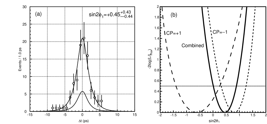
Figure 8: (a) The fitted proper-time difference distribution for all candidates : $\sum_{\eta_{f}=-1,+1}(dN/d(\eta_{f}\Delta t)|_{B^{0}}+dN/d(-\eta_{f}\Delta t)|_{\bar{B}^{0}})$. (b) The log-likelihoods for $CP+1$, $CP-1$, and both $CP\pm 1$.

Decay mode	$\sin 2\phi_{1}\;$
All $CP-1$ modes	$+0.81^{+0.44}_{-0.50}$
All $CP+1$ modes	$-0.61^{+0.87}_{-0.78}$
All $CP\pm 1$ modes	$+0.45^{+0.43}_{-0.44}$

Table 7: Results of the $C\!P$  fit

Source	$+\sigma$	$-\sigma$
Wrong tag fraction($\omega$)	$+0.050$	$-0.066$
Resolution function	$+0.026$	$-0.025$
Background shape	$+0.029$	$-0.042$
Background fraction	$+0.029$	$-0.032$
$\tau_{B^{0}}$, $\Delta m_{d}$	$+0.005$	$-0.006$
IP profile	$+0.004$	$-0.000$
Total	$+0.07$	$-0.09$

Table 8: Summary of the systematic errors on $\sin 2\phi_{1}\;$

2.2.7 Conclusion

We collected $6.2fb^{-1}$ of data on the $\Upsilon_{4S}$ by the end of the summer 2000. Using this data sample, we made a preliminary measurement of $\sin 2\phi_{1}\;$using $B\to J/\psi K_{S}(\pi^{+}\pi^{-})$, $B\to J/\psi K_{S}(\pi^{0}\pi^{0})$, $B\to\psi^{\prime}K_{S}(\pi^{+}\pi^{-})$, $B\to\chi_{C1}K_{S}(\pi^{+}\pi^{-})$, $B\to J\psi\pi^{0}$, and $B\to J/\psi K_{L}$. We found $\sin 2\phi_{1}\;$$=$ $+0.45^{+0.43}_{-0.44}$(stat.)${}^{+0.07}_{-0.09}$(syst.). Our result is consistent with the standard model prediction. We expect to improve the statistical errors as more data become available.

References

2.3 CP Violation in $B$-Decays at CDF: Results and Prospects.

Farrukh Azfar, Oxford University

2.3.1 Introduction

Charge-Parity (CP) violation in particle decays is necessary to explain the matter-anti-matter asymmetry observed in the universe today. The amount of Standard Model (SM) CP violation is too small to account for the observed asymmetry. A detailed study of CP violation provides us an excellent opportunity to search for physics beyond the Standard Model.

The CKM matrix

CP violation in the Standard model has its origins in the complex couplings of the Cabibbo-Kobayashi-Maskawa quark mixing matrix. The interference of various decay amplitudes are expected to give rise to large CP violating effects in the $B$ system.

The CKM matrix can be expressed in terms of 3 real parameters ($\rho$, $\lambda$, $A$) and one imaginary ($\eta$) parameter in a representation known as the Wolfenstein parameterization. This matrix is unitary and several orthogonality relations between its rows and columns can be derived. We represent one of these $V_{ud}V^{*}_{ub}+V_{cd}V^{*}_{cb}+V_{td}V^{*}_{tb}=0$, as a triangle in the complex plane.

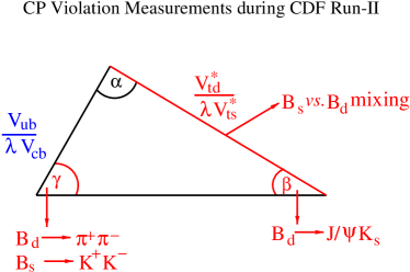
Figure 9: CDF plans for measuring the unitarity triangle (red).

At CDF we intend to measure one side and two angles of the unitarity triangle, by measuring the time dependent CP asymmetry in the modes $B_{d}^{0}\to\pi^{+}\pi^{-}$, $B_{s}^{0}\to K^{+}K^{-}$, $B_{d}^{0}\to J/\psi K_{S}^{0}$ and the $B_{s}^{0}-\bar{B}_{s}^{0}$ mixing parameter $x_{s}$ as illustrated in Fig. 9. A measurement of the time dependent CP asymmetry utilizing $B_{d}^{0}\to J/\psi K_{S}^{0}$ decays with 100 pb^-1 of data collected during Run-I has already been done at CDF [1].

The time dependent CP asymmetry will also be measured in modes where the SM asymmetry is expected to be small e.g. $B_{s}^{0}\to J/\psi\phi$ and $B_{s}^{0}\to D_{s}^{+}D_{s}^{-}$. A measurement of the width difference between the weak eigenstates of the $B_{s}^{0}$ is complimentary to such measurements and would utilize the same two modes. Comparisons of the width difference to the mixing parameter are also sensitive to non-SM Physics.

Mixing and CP violation in the neutral $B$ meson system

In $p-\bar{p}$ collisions $B$ and $\bar{B}$ mesons are created as strong interaction eigenstates which then “mix” into each other due to second order weak interactions represented by the box-diagram. The heavy and light weak interaction eigenstates are very nearly CP eigenstates each with its distinct mass and width, the quantities used to describe this two state system are: $M_{H}$, $M_{L}$, $\Gamma_{H}$, $\Gamma_{L}$, $\Delta M=M_{H}-M_{L}$, $\Delta\Gamma=\Gamma_{H}-\Gamma_{L}$, $\Gamma=\frac{\Gamma_{H}+\Gamma_{L}}{2}$, $\tau_{H,L}=\frac{1}{\Gamma_{H,L}}$ and $x_{d,s}=\frac{\Delta M_{d,s}}{\Gamma_{B_{d}^{0},B_{s}^{0}}}$.

If $B$ and $\bar{B}$ can decay to a CP eigenstate $\mid f>$, CP violation can occur if there is more than one amplitude contributing to the decay. If the complex CKM phases in both amplitudes are different then they will interfere causing an asymmetry in the rates $B\to\mid f>$ vs. $\bar{B}\to\mid f>$. The interference is caused by second order weak-interactions that are represented by the box or penguin diagrams.

Depending on whether we know (tag) the initial and final flavours of the $B$ and if the decay is to a CP eigenstate or a flavour specific final state, we will get a particular time evolution, these are summarized below:

• The flavour of the $B$ is unknown and the decay is to a CP eigenstate: $P(t)=\frac{e^{\frac{-t}{\tau_{L,H}}}}{\tau_{L,H}}$. Examples are $B_{s}^{0}\to D_{s}^{+}D_{s}^{-}$, $B_{d}^{0}\to\pi^{+}\pi^{-}$ (untagged).

• Flavour at birth is known, but not at decay, and the final state is a CP eigenstate: $P(t)\approx\frac{e^{(-\frac{t}{\tau_{L,H}})}}{\tau}(1\pm A_{CP}^{Mix}\sin\Delta Mt\pm A_{CP}^{Dir}\cos\Delta Mt)$ Examples: $B_{d}\to J/\psi K_{S}^{0}$, $A_{CP}^{Mix}=\sin 2\beta$, where $A_{CP}^{Dir}=0$, and $B_{d}^{0}\to\pi^{+}\pi^{-}$ $A_{CP}^{Mix}\neq 0$ and $A_{CP}^{Dir}\neq 0$, (tagged).

• Flavour at birth and at decay is known (mixing): $P(t)\approx\frac{e^{(-\frac{t}{\tau})}}{\tau}(1\pm\cos(\Delta Mt))$ Examples $B_{s}^{0}\to D_{s}^{\pm}l^{\mp}\nu(\bar{\nu})$ $B_{s}^{0}\to D_{s}^{\pm}\pi^{\mp}$, $B_{d}^{0}\to D^{\pm}l^{\mp}\nu(\bar{\nu})$.

Experimentally the path length before decay of the $B$ meson, $ct$ is measured.

2.3.2 The CDF detector, run-I and the run-II upgrade.

In this section, we briefly describe components of the CDF detector relevant to $B$-physics. A partially instrumented detector with several upgraded components, was tested with $p-\bar{p}$ collisions at a centre-of-mass energy of 2 TeV in October 2000. We expect the upgrade described to be completed by March 2001 [2]. The detectors present in Run-I are described along with their Run-II successors.

Tracking in the central region

Tracking in the Central Region is provided by wire drift chambers. In Run-I the Central Tracking Chamber (CTC) was used, this had $\approx$ 6000 axial and stereo sense wires with a transverse momentum resolution of $\frac{\delta P_{T}}{P_{T}^{2}}$ = 0.3 %, covering the region $-1\leq\eta\leq 1$. For Run-II the Central Outer Tracker (COT), with the same coverage and $P_{T}$ resolution will be used, this is already installed, and has $\approx$ 30,000 axial and stereo sense wires. The increased number of wires provide better $\frac{dE}{dx}$, somewhat improving particle identification.

Silicon microstrip detectors

Silicon Microstrip Detectors for precise vertex determination are needed for $B$ lifetime measurements. The Run-I Silicon Vertex detector (SVX), had four axial layers and a coverage of $-1\leq\eta\leq 1$. The proper decay length resolution was $\sigma_{c\tau}$: 35 $\mu$m = 0.12 ps. This detector provided measurements in the $r-\phi$ plane only. The Run-II Silicon Vertex Detector is known as the SVX-II, and has seven stereo and axial layers providing coverage in $-2\leq\eta\leq 2$ with an additional layer (Layer 00) at a distance of 1.4 cm from beam-pipe. Axial and Stereo strips provide the capability to do 3 dimensional tracking using only the SVX-II. The SVX-II $\sigma_{c\tau}$ is expected to be 15 $\mu$m = 0.045 ps.

Particle identification

A Time Of Flight (TOF) detector built from scintillators has been mounted on the outer surface of the COT, this provides us with some particle identification capability at low momenta. Differentiating kaons from pions is crucial for tagging the flavour of $B$s. In addition to the TOF, the coverage of the Muon Chambers has been extended from $\eta=$1.0 in Run-I to $\eta=$ 1.4. High momentum muons are easily identified, and allow us to select events with $b\to\mu\nu_{\mu}X$ and $b\to c\bar{c}$ with $c\bar{c}\to J/\psi\to\mu^{+}\mu^{-}$.

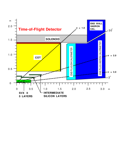
Figure 10: A side view of the CDF detector.

2.3.3 Triggers and data selection

At the Tevatron with $p-\bar{p}$ collisions at a centre-of-mass energy of $1.8$TeV the $b$ production cross-section is $\sigma_{b\bar{b}}=$100$\mu$b, however the inelastic cross section is three orders of magnitude higher. Although $\sigma_{b\bar{b}}$ is much higher than for $e^{+}-e^{-}$ at the $\Upsilon(4S)$ and $Z$ resonances (1 and 7 nb), the high inelastic cross section requires specialized triggers for the selection of $b\bar{b}$ events.

CDF run-I triggers

The selection of $b\bar{b}$ events during Run-I at CDF relied on high transverse momentum ($P_{T}$) leptons. The inclusive lepton $\ell=(\mu,e)$ trigger selected events with $P_{T}(B)>$8 GeV, the quark level decays being $b\to\ell\nu cX$ or $b\to cX$ $c\to\ell\nu X$. Dilepton triggers selected $(\mu e)$ and $(\mu\mu)$ events with $P_{T}(B)\approx$10 GeV were also in use. These were crucial in selecting $b\to J/\psi X$ with $J/\psi\to\mu\mu$ and $b\to\mu^{-}X$, $\bar{b}\to e^{+}X$. The $\sin 2\beta$ analysis requires the reconstruction of the mode $B_{d}^{0}\to J/\psi K_{S}^{0}$, for which the data sample was selected using the $J/\psi\to\mu^{+}\mu^{-}$ trigger. The long-lifetime of $B$ mesons was not utilized in any trigger during Run-I.

In Run-I the single lepton trigger data samples were used to measure $B_{d}^{0}$ mixing. The presence of a neutrino in the final state introduces uncertainties in the $B$ decay vertex determination. Despite this the CDF measurement of the $B_{d}^{0}$ mixing parameter $x_{d}=$ 0.77 $\pm$ 0.040 compares well with world average $x_{d}$= 0.739 $\pm$ 0.023 [3]. However this uncertainty will degrade the $B_{s}^{0}$ mixing parameter $x_{s}$ measurement significantly, since the oscillation period is much smaller. Clearly it is crucial to be able to trigger on fully reconstructible modes.

CDF run-II triggers

The Run-II CDF triggers used to select $B$ decays will include all Run-I triggers, in addition a new high impact parameter track trigger using SVX-II hit information will be used in order to select displaced hadronic tracks from $B$ decays. Therefore in Run-II CDF it will be possible to select $B$ decays with fully reconstructible purely hadronic decay states, such as $B_{s}^{0}\to D_{s}^{+}D_{s}^{-}$, $B_{d}^{0}\to\pi^{+}\pi^{-}$ and $B_{s}^{0}\to D_{s}^{\pm}\pi^{\mp}$. These decays allow us to measure the $B_{s}^{0}$ width difference and mixing.

2.3.4 The CP asymmetry, $\sin 2\beta$ in $B_{d}^{0}\to J/\psi K_{S}^{0}$: run-I

To measure the CP asymmetry in $B_{d}^{0}\to J/\psi K_{S}^{0}$, the flavour of the $B_{d}^{0}$ at production has to be tagged, and the decay fully reconstructed. The tagging of the flavour is neither fully efficient nor correct each time, we define the dilution variable $D=\frac{N_{R}-N_{W}}{N_{R}+N_{W}}$ where $N_{R}$ and $N_{W}$ are the number of correct and incorrect tags. If the tagging efficiency is given by $\epsilon$ then a CP asymmetry measured using $N$ tagged events will have the statistical power of $\epsilon D^{2}N$ fully efficiently and correctly tagged events.

Flavour tagging: opposite and same side

Opposite side tagging algorithms use decay products from the $b$ quark on the opposite side of the reconstructed decay of interest. The decay products used are the jet associated with the hadronization of the $b$ into a $B$ or the sign of the lepton in case the $B$ decays leptonically. In case of non-leptonic decays a weighted sum of charges of all tracks is used to tag the $B$ flavour. The lepton tagging is known as the Soft Lepton Tag, has high dilution but low efficiency, the figure of merit, $\epsilon D^{2}$ is 0.91 $\pm$ 0.1 %. The Jet Charge technique is more efficient but has worse dilution, with $\epsilon D^{2}$= 0.78 $\pm$ 0.12 %.

There are two disadvantages of the opposite side tagging techniques: the opposite $B$ is within detector acceptance only 40 % of the time, and if the opposite $B$ is neutral then it may have mixed. These factors degrade efficiency and dilution.

The same side tagging (SST) algorithm uses the hadronization products on the same side as the reconstructed decay to determine the flavour of the $B$. This has a figure of merit $\epsilon D^{2}$= 1.8 $\pm$ 0.4%, as measured in Run-I.

Results from run-I

The candidate events for reconstructing the decay $B_{d}^{0}\to J/\psi K_{S}^{0}$ with $J/\psi\to\mu^{+}\mu^{-}$ and $K_{S}^{0}\to\pi^{+}\pi^{-}$ were selected using the Run-I $J/\psi\to\mu^{+}\mu^{-}$ trigger. Roughly 400 such events were reconstructed with some 200 within the acceptance of the SVX. The tagging algorithms described were tested and tuned on a sample of $B_{u}^{\pm}\to J/\psi K^{\pm}$ decays, and the dilutions determined. The flavour of the $B$ is already known in this decay mode, so it can be used for tuning the algorithms.

All 400 events were used in an unbinned likelihood multi-parameter fit of the mass and decay length distributions, and tag information of the reconstructed $B_{d}^{0}\to J/\psi K_{S}^{0}$ decays, each tagging algorithm was used for each event with an appropriate weighting accounting for agreement or disagreement between the taggers.

The reconstructed mass spectrum and time dependent asymmetry for $B_{d}^{0}\to J/\psi K_{S}^{0}$ are shown in Fig. 11. The best fit value of the parameter $\sin 2\beta$ is 0.79 $\pm$ 0.39 (stat) $\pm$ 0.16(sys) where the systematic error is dominated by uncertainties in the dilution.

Figure 11: Mass spectrum of $B_{d}^{0}\to J/\psi K_{S}^{0}$ decays, signal: 395 $\pm$ 31 (left) and the CP asymmetry as a function of time (right).

2.3.5 Prospects for run-II

The plan for Run-II is to constrain the unitarity triangle by measuring one side using $B_{s}^{0}$ mixing, two angles $\gamma$ using CP asymmetries in $B_{d}^{0}\to\pi^{+}\pi^{-}$ and $B_{s}^{0}\to K^{+}K^{-}$ and $\beta$ ($\sin 2\beta$), as in Run-I, by measuring the asymmetry in $B_{d}^{0}\to J/\psi K_{S}^{0}$, this is shown in Fig. 9.

Preparing the ground for projections

We expect at least 2fb^-1 of data in Run-II which is a factor of 20 higher than Run-I, this figure has been used as the basis for all projections in this article, it is important to note that this is a very conservative estimate, the laboratory director’s recent stated goal being 15 fb^-1.

In addition to the increase in luminosity, the increased coverage of the SVX-II and Muon chambers will increase our statistics for all Run-I modes by a factor of 50-60.

All Run-I analyses such as the CP asymmetry in $B_{d}^{0}\to J/\psi K_{S}^{0}$ will be repeated with much higher statistics and several new modes, selected using the hadronic displaced track trigger will be used to search for CP violation and $B_{s}^{0}$ mixing.

$\sin 2\beta$ in run-II

We expect at least 10,000 events in the channel $B_{d}^{0}\to J/\psi K_{S}^{0}$, therefore the statistical error $\sigma_{\sin 2\beta}$ will be $\approx$ 0.067. We expect a similar decrease in the systematic error, since it is dominated by errors in measuring dilution, due to the larger $B_{u}^{\pm}\to J/\psi K^{\pm}$ calibration sample. We have not included the contribution of other decays that the hadronic displaced track trigger will select: such as $B_{d}^{0}\to D^{*+}D^{*-}$, $B_{d}^{0}\to D^{+}D^{-}$ and $B_{d}^{0}\to\phi K_{S}^{0}$, where the time dependent CP asymmetry is also proportional to $\sin 2\beta$.

$\gamma$ using $B_{d}^{0}\to\pi^{+}\pi^{-}$ and $B_{s}^{0}\to K^{+}K^{-}$

In the absence of penguin-graphs the asymmetry in the decay $B_{d}^{0}\to\pi^{+}\pi^{-}$ will measure $\sin 2(\gamma+\beta)$ and similarly the asymmetry in the decay $B_{s}^{0}\to K^{+}K^{-}$ should only measure $\sin 2\gamma$. However penguins are present in both decays, the $\pi^{+}\pi^{-}$ mode is tree dominated the $K^{+}K^{-}$ mode is penguin dominated. The CP asymmetry for $B_{d}^{0}\to\pi^{+}\pi^{-}$ is $A_{CP,\pi^{+}\pi^{-}}^{dir}\cos\Delta M_{d}t+A_{CP,\pi^{+}\pi^{-}}^{mix}\sin\Delta M_{d}t$ and for the mode $B_{s}^{0}\to K^{+}K^{-}$ it is $A_{CP,K^{+}K^{-}}^{dir}\cos\Delta M_{s}t+A_{CP,K^{+}K^{-}}^{mix}\sin\Delta M_{s}t$. The four $A_{CP}$ terms can be expressed in terms of 4 parameters, $d$ the ratio of the penguin to tree amplitudes (assuming SU(3) symmetry), $\theta$ the ratio of the phases of the penguin and tree amplitudes, and the CKM angles $\gamma$ and $\beta$. These can be solved for by using the 4 asymmetries and the measurement of $\sin 2\beta$ [4]. We expect the hadronic displaced track trigger to select 5000 $B_{d}^{0}\to\pi^{+}\pi^{-}$ and 10000 $B_{s}^{0}\to K^{+}K^{-}$, and a simulation based on these estimates was performed. An estimated SU(3) breaking of 20 % was put into the simulation and the resulting inaccuracy is part of the combined systematic and statistical error of 10 degrees in measuring $\gamma$. All estimates of background were based on Run-I data.

Determination of $x_{s}$ the $B_{s}^{0}$ mixing parameter

The ratio of the mixing parameters $\frac{x_{d}}{x_{s}}$ of the $B_{d}^{0}$ and $B_{s}^{0}$ neutral mesons is proportional to $\frac{\mid V_{ts}\mid^{2}}{\mid V_{td}\mid^{2}}$. Since $V_{ts}>>$ $V_{td}$, the $B_{s}^{0}$ oscillates much faster than the $B_{d}^{0}$, and we expect $x_{s}\approx 25$ ($x_{d}\approx$=0.75)

The measurement of $x_{s}$ oscillation is challenging. In Run-I we measured the oscillation parameter of the $B_{d}^{0}$ meson, this means measuring an oscillation of period 2.12 ps with a $ct$ resolution of 0.1 ps. To measure the $x_{s}$ we will try to measure a period of 0.07 ps with the SVX-II resolution of 0.045ps.

We expect 20,000 $B_{s}^{0}\to D_{s}^{\pm}\pi^{\mp}$ and $B_{s}^{0}\to D_{s}^{\pm}\pi^{\mp}\pi^{\mp}\pi^{\pm}$ with $D_{s}^{\pm}\to\phi\pi^{\pm}$ which the hadronic trigger will select. We have estimated our accuracy for measuring $x_{s}$ with a signal to noise of 2:1 and 1:2 based on Run-I estimates. We expect to measure a $x_{s}$ of up to 63 with a significance of 5$\sigma$. This accuracy in measuring $x_{s}$ corresponds to an accuracy of 7 % in measuring $\mid\frac{V_{td}}{\lambda V_{ts}}\mid$. In addition to measuring this side of the unitarity triangle the value of $x_{s}$ can be used as a constraint in CP asymmetry measurements in CP violating $B_{s}^{0}$ decays.

2.3.6 Non-SM surprises from the $B_{s}^{0}$ width difference and CP violation in $B_{s}^{0}$ decays

In the standard model the $B_{s}^{0}$ width difference $\Delta\Gamma$ can be written in a CKM independent form in terms of the top, bottom, W and charm masses and the $B_{s}^{0}$ mixing parameter $x_{s}$ [5]. The fractional width splitting between the light and heavy $B_{s}^{0}$ $\frac{\Delta\Gamma}{\Gamma}$ is expected to be large $\approx$ 0.15. If we measure both $x_{s}$ and $(\frac{\Delta\Gamma}{\Gamma})_{B_{s}^{0}}$ we can test the SM prediction. In particular, we are interested in cases where $x_{s}$ is too large to measure but $\frac{\Delta\Gamma}{\Gamma}$ is measurable or conversely, if $\frac{\Delta\Gamma}{\Gamma}$ is too small to measure and $x_{s}$ is measurable. In the presence of new Physics a non-SM CP violating phase $\phi_{BSM}$ can appear, and will reduce the width difference: $\Delta\Gamma_{Measured}=\Delta\Gamma_{SM}\cos\phi_{BSM}$. Complimentary to this effect the CP asymmetry in modes such as $B_{s}^{0}\to J/\psi\phi$ will be proportional to $\sin 2\phi_{BSM}$.

In Run-I approximately 60 $B_{s}^{0}\to J/\psi\phi$ decays were reconstructed from a data sample selected using the $J/\psi\to\mu^{+}\mu^{-}$ trigger and a single lifetime was measured [6]. The final state $J/\psi\phi$ is however to a mixture of CP even and odd final states, it therefore contains two lifetimes, for the heavy ($\approx$ CP odd) and light ($\approx$ CP even) $B_{s}^{0}$ states. Using angular variables to disentangle the CP content of the final state we can fit for two lifetimes utilizing a likelihood function normalized over invariant mass, lifetime and the angular variable [7]. We expect a signal of 4000 $B_{s}^{0}\to J/\psi\phi$ in Run-II. A simulation based on 4000 signal events and Run-I observations of signal and background shapes has been used to predict that we can measure a $(\frac{\Delta\Gamma}{\Gamma})_{B_{s}^{0}}$ of 0.15 with a precision of 0.05. This does not include any contribution from the purely CP even mode $B_{s}^{0}\to D_{s}^{+}D_{s}^{-}$ which will be selected using the hadronic displaced track trigger, the lifetime measured in this mode can be compared with the results of a single-lifetime fit to semi-leptonic $B_{s}^{0}$ decays and $(\frac{\Delta\Gamma}{\Gamma})_{B_{s}^{0}}$ can be extracted.

The SM prediction for CP asymmetry in the $B_{s}^{0}\to D_{s}^{+}D_{s}^{-}$ and $B_{s}^{0}\to J/\psi\phi$ modes is of order 3%, we do not expect to be able to see this at CDF, however if there are non-SM sources of CP violation, we may be able to observe this, by doing a conventional tagging analysis in $B_{s}^{0}\to D_{s}^{+}D_{s}^{-}$ and a tagging analysis of the disentangled CP states of $B_{s}^{0}\to J/\psi\phi$.

2.3.7 Conclusion

During Run-II at CDF we have been able to measure of $\sin 2\beta=$0.79 $\pm$ 0.39 (stat) $\pm$ 0.16(sys) and the $B_{d}^{0}$ mixing parameter $x_{d}$ $=$ 0.77 $\pm$ 0.040(stat) $\pm$0.039 (syst), and have fully reconstructed the largest sample of $B_{s}^{0}$ decays.

Thus the viability of a rich CP violation program for Run-II, during which we expect a factor of 50 increase in data, has been established. The introduction of the displaced track trigger will allow us to select fully reconstructible hadronic modes of all $B$ mesons. We expect to be able to constrain one side and two angles of the unitarity triangle. We expect to measure $\mid\frac{V_{td}}{\lambda V_{ts}}\mid$ to $\approx$ 7% accuracy, using $B_{s}^{0}$ mixing. We emphasize that for the next few years CDF is unique in its ability to analyse $B_{s}^{0}$ decays. We expect to use $B_{d}^{0}\to\pi^{+}\pi^{-}$, $B_{s}^{0}\to K^{+}K^{-}$ to measure $\gamma$ with a precision $\sigma_{\gamma}\approx 10^{o}$, and using $B_{d}^{0}\to J/\psi K_{S}^{0}$ to measure $\sin 2\beta$ to a precision of 0.067.

References

2.4 B physics potential of future experiments at hadron machines

V Gibson, Cambridge

2.4.1 Introduction

CP violation remains one of the enigmas of particle physics today. Experimentalists have just started a full programme of research to study CP violation in B decays. The experiments can be divided into two phases. The main goal of the current phase of experiments will be to observe CP violation in the B system in the exciting exploratory phase, with the potential to establish a breakdown in the Standard Model [1]. This review concentrates on the next generation of experiments which become operational around 2006. The experiments considered are the dedicated B physics experiments, LHCb [2] at the Large Hadron Collider (LHC) and the proposed BTeV experiment [3] at the Tevatron, as well as the general purpose experiments ATLAS [4] and CMS [5] at the LHC. The main aims of these experiments will be to make precision measurements of CP violating observables using many different decay channels and species of $\mathrm{B}$ hadrons. They will thoroughly test the internal consistency of the Standard Model description of CP violation and have the sensitivity to search for the necessary new physics beyond.

CP violation in the Standard Model and beyond

CP violation arises naturally in the Standard Model through the presence of a single phase in the unitary Cabibbo-Kobayashi-Maskawa ($\mathrm{CKM}$) quark-mixing matrix [6]. The unitarity of the $\mathrm{CKM}$ matrix is clearly exposed when using an explicit parameterization. A very popular parameterization is the perturbative form suggested by Wolfenstein [7], which can be expanded to order $\lambda^{5}$ ($\lambda\equiv\sin\theta_{C}\sim 0.22$ where $\theta_{C}$ is the Cabibbo angle):

$$V_{\mathrm{CKM}} = \left(\begin{array}[]{ccc}1-\frac{1}{2}\lambda^{2}&\lambda&A\lambda^{3}(\rho-i\eta)\\ -\lambda&1-\frac{1}{2}\lambda^{2}&A\lambda^{2}\\ A\lambda^{3}(1-\rho-i\eta)&-A\lambda^{2}&1\end{array}\right)$$ (19)

$$+ \left(\begin{array}[]{ccc}0&0&0\\ -iA^{2}\lambda^{5}\eta&0&0\\ A\lambda^{5}(\rho+i\eta)/2&A\lambda^{4}(1/2-\rho-i\eta)&0\end{array}\right).$$

The parameter $\eta$ represents the CP violating phase in the Standard Model and appears in three of the matrix elements. The unitarity of the CKM matrix implies that there are six orthogonality conditions, which can be represented geometrically as triangles in the complex plane. Two such unitarity triangles, shown in Figure 12, are expected to have angles, which are all non-trivial.

The angles of the unitarity triangles are all related to the single CP-violating phase in the $\mathrm{CKM}$ matrix and are designated by $\alpha$, $\beta$, $\gamma$ and $\delta\gamma$;

$$\beta=\tan^{-1}\left[\frac{\eta(1-\lambda^{2}/2)}{1-\rho(1-\lambda^{2}/2)}\right],\;\;\;\gamma=\tan^{-1}\frac{\eta}{\rho},\;\;\;\delta\gamma=\eta\lambda^{2},$$

and $\alpha=\pi-\beta-\gamma$. The angles $\beta,\delta\gamma$ and $\gamma$ are commonly referred to as the $\mathrm{B}^{0}_{\mathrm{d}}$ mixing phase, the $\mathrm{B}^{0}_{\mathrm{s}}$ mixing phase and the weak decay phase respectively. By 2006, it is expected that a measurement of $\sin 2\beta$ will have been made with a precision of $\sim 0.02$ [8]. There will be no good or direct measurement of $\gamma$ and there will be no sensitivity to $\delta\gamma$.

Figure 12: The unitarity triangles characterized by the relations $V_{ud}V_{ub}^{*}+V_{cd}V_{cb}^{*}+V_{td}V_{tb}^{*}=0$ and $V_{ud}V_{td}^{*}+V_{us}V_{ts}^{*}+V_{ub}V_{tb}^{*}=0$. The phase convention is chosen such that $V_{cd}V_{cb}^{*}$ is real and all sides are normalized to $|V_{cd}V_{cb}^{*}|$.

It is expected that the single Standard Model $\mathrm{CKM}$ phase is insufficient to explain the observed baryon asymmetry in the universe [9] and that new physics must intervene. A large source of CP violation at the electroweak scale could be provided for in extensions to the Standard Model [10]. A summary of physics beyond the Standard Model and its effects on the $\mathrm{CKM}$ parameters can be found in references [11, 12]. In order to search for new physics it is essential to measure and calculate as many processes as possible and to compare the resulting $\mathrm{CKM}$ parameters with each other.

The next generation experiments

The LHC and Tevatron colliders will provide an intense source of the full spectrum of B hadrons $(\mathrm{B}^{\pm},\,\mathrm{B}^{0}_{\mathrm{d}},\,\mathrm{B}^{0}_{\mathrm{s}},\,\mathrm{B}^{\pm}_{\mathrm{c}}$ and b-baryons). The running parameters of the colliders and experiments are given in Table 9. The expected cross-section for the production of $\mathrm{b}\bar{\mathrm{b}}$ pairs at the LHC is approximately five times that expected at the Tevatron, with a relatively smaller inelastic cross-section.

	Tevatron	LHC
Energy/collision mode	2.0 TeV $p\bar{p}$	14.0 TeV $pp$
$\mathrm{b}\bar{\mathrm{b}}$ cross-section	$\sim 100\mu$b	$\sim 500\mu$b
Inelastic cross-section	$\sim 50$mb	$\sim 80$mb
Ratio $\mathrm{b}\bar{\mathrm{b}}$/inelastic	0.2%	0.6%
Bunch spacing	132 ns	25 ns
Bunch length	$\sim 30$cm	$\sim 5$cm
	BTeV	LHCb	ATLAS/ CMS
Detector configuration	Two-arm forward	Single-arm forward	Central detector
Running luminosity	$1.5\times 10^{32}\,\mathrm{cm}^{-2}\mathrm{s}^{-1}$	$1.5\times 10^{32}\,\mathrm{cm}^{-2}\mathrm{s}^{-1}$	$1\times 10^{33}\,\mathrm{cm}^{-2}\mathrm{s}^{-1}$
$\mathrm{b}\bar{\mathrm{b}}$ events per $10^{7}$ sec	$2\times 10^{11}\times accep$	$1\times 10^{12}\times accep$	$5\times 10^{12}\times accep$
$\langle$Interactions/crossing$\rangle$	$\sim 2.0$	$\sim 0.5$ (30% single int.)	$\sim 2.3$
Mass resolution $\mathrm{B}^{0}_{\mathrm{d}}\rightarrow J/\psi\mathrm{K}^{0}_{\mathrm{S}}$	9.3 $\mathrm{MeV}/\mathrm{c}^{2}$	7 $\mathrm{MeV}/\mathrm{c}^{2}$	18/16 $\mathrm{MeV}/\mathrm{c}^{2}$
Proper time res. $\mathrm{B}^{0}_{\mathrm{s}}\rightarrow\mathrm{D}_{\mathrm{s}}^{\pm}\pi^{\mp}$	43 fs	43 fs	50/65 fs

Table 9: Comparison of the LHC and Tevatron collider running parameters and experiments.

The forward detector geometries of the LHCb and BTeV experiments exploit the expected forward peaked and strongly correlated production of $\mathrm{b}$ and $\bar{\mathrm{b}}$ hadrons. LHCb is instrumented on one arm with a dipole spectrometer [2] and is designed to run at a low LHC luminosity of $1.5\times 10^{32}\,\mathrm{cm}^{-2}\mathrm{s}^{-1}$. It employs a precision ministrip silicon detector and has an efficient multi-level trigger, which includes a vertex, trigger at the second level. The experiment employs two RICH detectors for particle identification and has hadronic and electromagnetic calorimetry. The key design features of the BTeV detector include a forward two-arm spectrometer, a precision silicon pixel vertex detector, a vertex trigger at the first level, a RICH detector and a lead-tungstate calorimeter for neutral particle reconstruction [3]. The geometrical acceptance, the use of a vertex trigger at the first level and of multi-bunch interactions mostly compensate for the smaller $\mathrm{b}\bar{\mathrm{b}}$ cross-section at the Tevatron. ATLAS and CMS are central detectors designed for general-purpose use at the LHC [4, 5]. During the first three years of running, the LHC will operate at a low luminosity, $1\times 10^{33}\,\mathrm{cm}^{-2}\mathrm{s}^{-1}$, thereby enabling ATLAS and CMS to pursue a B physics programme. ATLAS and CMS have tracking capabilities in the central region and employ precision silicon pixel and microstrip detectors. Specialist $\mathrm{B}$ triggers are achieved by reducing the lepton $p_{T}$ thresholds to a minimum.

The requirements of the dedicated experiments are governed by the need to measure time-dependent CP asymmetries for $\mathrm{B}$ and $\overline{\mathrm{B}}$ hadrons decaying to the same final state. The experimental acceptance and trigger efficiencies mainly cancel. However, precise measurements require good decay time and mass resolutions, efficient triggers for low and high multiplicity $\mathrm{B}$ final states, particle identification for $\pi/\mathrm{K}$ separation and photon detection for neutral final states. An example of the $\mathrm{B}^{0}_{\mathrm{d}}\rightarrow J/\psi\mathrm{K}^{0}_{\mathrm{S}}$ mass resolution is given in Table 9. The flavour of the $\mathrm{B}$ hadron at production needs to be determined either using the signal $\mathrm{B}$ or the other $\mathrm{B}$ in the event and good control of systematic uncertainties is crucial [12]. The experimental need for good flavour tagging and $\mathrm{B}$ proper time resolution is demonstrated through the measurement of $\mathrm{B}^{0}_{\mathrm{s}}$ oscillations. The bench-mark decay mode for this measurement is $\mathrm{B}^{0}_{\mathrm{s}}\rightarrow\mathrm{D}_{\mathrm{s}}^{\pm}\pi^{\mp}$ in which the flavour of the $\mathrm{B}^{0}_{\mathrm{s}}$ is given by the charge of the $\mathrm{D}_{\mathrm{s}}$. The proper time resolutions obtained by the experiments is summarised in Table 9. The event yields and expected measurable values for the $\mathrm{B}^{0}_{\mathrm{s}}$ mixing parameter are given in Table 10.

2.4.2 Direct measurements of CKM angles and search for new physics

The internal consistency of the Standard Model description of quark mixing in weak interactions can be thoroughly tested by measuring CP violating observables in the decays of B mesons. If the Standard Model is correct then all such measurements will be describable with a single set of CKM parameters. New physics outside the Standard Model could lead to additional phases in the CKM matrix and an inconsistency between the measurements. This review discusses the current status of studies performed by the new generation experiments to extract the CKM angles $\alpha,\beta,\gamma$ and $\delta\gamma$. The event yields and sensitivities presented are mainly taken from references [3] and [12] where further details can be found. Since the experiments are at different stages in their preparation for physics, the results quoted should only be considered as a current snapshot.

$\mathrm{B}^{0}_{\mathrm{d}}$ mixing phase

The decay $\mathrm{B}^{0}_{\mathrm{d}}\rightarrow J/\psi\mathrm{K}^{0}_{\mathrm{S}}$ is a transition into a CP eigenstate and is dominated by only one CKM amplitude. Hence, the time-dependent CP asymmetry is governed by the $\mathrm{B}^{0}_{\mathrm{d}}$ mixing phase, $\beta$. The decay is also experimentally clean and can be reconstructed with relatively low backgrounds. Examples of the $\mathrm{B}^{0}_{\mathrm{d}}\rightarrow J/\psi\mathrm{K}^{0}_{\mathrm{S}}$ reconstructed mass distribution and CP asymmetry are shown in Figure 13. The expected event yields and sensitivities for the next generation experiments are given in Table 10. Ultimately, a combined statistical precision of 0.005 should be achievable at the LHC.

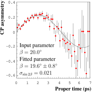
Figure 13: The ATLAS $\mathrm{B}^{0}_{\mathrm{d}}\rightarrow J/\psi\mathrm{K}^{0}_{\mathrm{S}},\;J/\psi\rightarrow e^{+}e^{-}$ reconstructed mass distribution after 3 years of data and the LHCb CP asymmetry with one year’s data.

The $\mathrm{B}^{0}_{\mathrm{s}}$ mixing phase

The decays $\mathrm{B}^{0}_{\mathrm{s}}\rightarrow J/\psi\phi$ and $\mathrm{B}^{0}_{\mathrm{s}}\rightarrow J/\psi\eta^{(\prime)}$ are $\mathrm{B}^{0}_{\mathrm{s}}$ counterparts to the decay mode $\mathrm{B}^{0}_{\mathrm{d}}\rightarrow J/\psi\mathrm{K}^{0}_{\mathrm{S}}$. Once again these decays are dominated by only one CKM amplitude and are sensitive to the $\mathrm{B}^{0}_{\mathrm{s}}$ mixing phase, $\delta\gamma$. Experimentally, the decay mode $\mathrm{B}^{0}_{\mathrm{s}}\rightarrow J/\psi\phi$ is very clean, but requires a full angular analysis to disentangle the mixture of CP eigenstates in the final state. The reconstruction of the decay $\mathrm{B}^{0}_{\mathrm{s}}\rightarrow J/\psi\eta^{(\prime)}$ benefits from good electromagnetic calorimetry and, because it is a transition into a CP eigenstate, the $\delta\gamma$ can be extracted directly from the decay asymmetry. The expected sensitivities of the experiments for the extraction of $\delta\gamma$ are summarised in Table 10 and depend strongly on the proper time resolution and $\mathrm{B}^{0}_{\mathrm{s}}$ mixing parameter. It is interesting to note that the expected sensitivity for the extraction of $\delta\gamma$ from $\mathrm{B}^{0}_{\mathrm{s}}\rightarrow J/\psi\eta^{(\prime)}$ decays in one year of running (BTeV) is comparable to 5 years of running for the full angular analysis of $\mathrm{B}^{0}_{\mathrm{s}}\rightarrow J/\psi\phi$ (LHCb). It has been suggested that some of this difference can be recuperated using a transversity angle analysis [13]. A particularly interesting feature of these decays is that they exhibit very small CP violating effects within the Standard Model, $\delta\gamma=\lambda^{2}\eta\approx 0.03$, and hence are very sensitive to new physics (see [12] and references therein).

The angle $\alpha$

$\mathrm{B}^{0}_{\mathrm{d}}\rightarrow\rho^{\pm}\pi^{\mp}$:

A full three-body analysis of the decay $\mathrm{B}^{0}_{\mathrm{d}}\rightarrow\pi^{+}\pi^{-}\pi^{0}$ in the $\rho$ resonance region, taking into account interference effects between vector mesons of different charges, has been proposed to extract all parameters that describe both the tree and penguin contributions to $\mathrm{B}^{0}_{\mathrm{d}}\rightarrow\rho^{\pm}\pi^{\mp}$, including the CKM angle $\alpha$ [14]. Although the method is theoretically clean, it is experimentally difficult due to the need to reconstruct $\pi^{0}$’s and the presence of a large combinatorial background. The invariant mass for $\mathrm{B}^{0}_{\mathrm{d}}\rightarrow\rho^{0}\pi^{0}$ candidates reconstructed in BTeV and the $\pi^{+}\pi^{-}\pi^{0}$ Dalitz plot from LHCb are shown in Figure 14. The event yields, given in Table 10, are expected to be sufficient, so that an unambiguous value for $\alpha$ can be extracted.

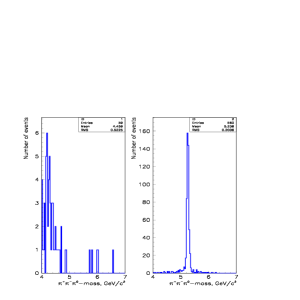
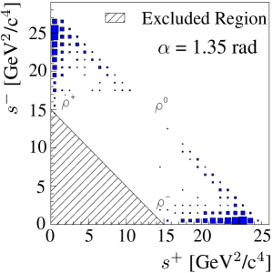
Figure 14: The $\pi^{+}\pi^{-}\pi^{0}$ invariant mass distribution for background and signal events for $\mathrm{B}^{0}_{\mathrm{d}}\rightarrow\rho^{0}\pi^{0}$ decays from BTeV and the LHCb Dalitz plot.

$\mathrm{B}^{0}_{\mathrm{d}}\rightarrow\pi^{+}\pi^{-}$:

In principle, the decay mode $\mathrm{B}^{0}_{\mathrm{d}}\rightarrow\pi^{+}\pi^{-}$ allows the $\mathrm{CKM}$ angle $\alpha$ to be probed. However, penguin contributions to the transition amplitude introduce a direct CP violation contribution, $A^{dir}_{\mathrm{CP}}$, into the decay asymmetry,

$$A(t)=A^{dir}_{\mathrm{CP}}\cos(\Delta Mt)+A^{mix}_{\mathrm{CP}}\sin(\Delta Mt).$$

Experimentally, the analysis of $\mathrm{B}^{0}_{\mathrm{d}}\rightarrow\pi^{+}\pi^{-}$ decays is complicated by the existence of backgrounds with similar topologies and with unknown CP asymmetries, such as $\mathrm{B}^{0}_{\mathrm{d}}\rightarrow\pi^{+}\mathrm{K}^{-}$, $\mathrm{B}^{0}_{\mathrm{s}}\rightarrow\mathrm{K}^{+}\mathrm{K}^{-}$, $\mathrm{B}^{0}_{\mathrm{s}}\rightarrow\pi^{+}\mathrm{K}^{-}$, $\Lambda_{\mathrm{b}}\rightarrow\mathrm{p}\pi^{-}$ and $\Lambda_{\mathrm{b}}\rightarrow\mathrm{p}\mathrm{K}^{-}$. This is illustrated in Figure 15 (left) which shows the reconstructed two pion invariant mass distribution obtained in ATLAS. In order to reject the non $\pi^{+}\pi^{-}$ background, LHCb exploits the powerful RICH particle identification detectors, shown in Figure 15 (centre). The expected $\mathrm{B}^{0}_{\mathrm{d}}\rightarrow\pi^{+}\pi^{-}$ event yields and the experimental sensitivities for the CP observables are given in Table 10. The observables can be written to leading order in the ratio of penguin to tree amplitudes, $\left|\mathrm{P}/\mathrm{T}\right|$,

$$A^{mix}_{\mathrm{CP}}=-\sin 2\alpha-2\left|\frac{\mathrm{P}}{\mathrm{T}}\right|\sin\alpha\cos 2\alpha\cos(\delta),\;\;\;A^{dir}_{\mathrm{CP}}=2\left|\frac{\mathrm{P}}{\mathrm{T}}\right|\sin\alpha\sin(\delta),$$

where $\delta$ is the CP conserving strong phase, $\delta=arg(PT^{*})$. Unfortunately, a theoretically reliable prediction for $\left|\mathrm{P}/\mathrm{T}\right|$ which would allow the extraction of $\alpha$, albeit with a four-fold discrete ambiguity, is very challenging. Figure 15 (right) shows the expected sensitivity to $\alpha$ for different values of the uncertainty on $\left|\mathrm{P}/\mathrm{T}\right|$ and integrated luminosities. It can be seen that for values of $\alpha$ around $90^{\circ}$, the sensitivity to $\alpha$ is already limited after one year of running, if the uncertainty on $\left|\mathrm{P}/\mathrm{T}\right|$ is not better than $10\%$.

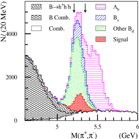
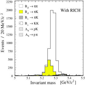
Figure 15: The ATLAS $\pi^{+}\pi^{-}$ invariant mass distribution (left), the LHCb $\pi^{+}\pi^{-}$ invariant mass distribution after the application of RICH information (centre) and the expected LHC combined sensitivity to $\alpha$ as a function of $\alpha$ (right), for $\delta=30^{\circ}$, $\left|\mathrm{P}/\mathrm{T}\right|=0.2$ after one year (dashed lines) and 5 years (solid lines).

The weak decay phase $\gamma$

$\mathrm{B}^{0}_{\mathrm{d}}\rightarrow\pi^{+}\pi^{-}$ and $\mathrm{B}^{0}_{\mathrm{s}}\rightarrow\mathrm{K}^{+}\mathrm{K}^{-}$:

A strategy has been proposed to combine the CP observables from the decay $\mathrm{B}^{0}_{\mathrm{d}}\rightarrow\pi^{+}\pi^{-}$ with those from $\mathrm{B}^{0}_{\mathrm{s}}\rightarrow\mathrm{K}^{+}\mathrm{K}^{-}$ to provide a simultaneous determination of the angles $\beta$ and $\gamma$ [15]. The decays $\mathrm{B}^{0}_{\mathrm{d}}\rightarrow\pi^{+}\pi^{-}$ and $\mathrm{B}^{0}_{\mathrm{s}}\rightarrow\mathrm{K}^{+}\mathrm{K}^{-}$ are related to each other by interchanging all down and strange quarks (U-spin symmetry). Assuming the $\mathrm{B}^{0}_{\mathrm{s}}$ mixing phase $\delta\gamma$ is known, the four observables, depend on four unknowns: two hadronic parameters, the $\mathrm{B}^{0}_{\mathrm{d}}$ mixing phase $\beta$ and the weak phase $\gamma$. If $\beta$ is also fixed from external measurements then the weak phase, $\gamma$, can be extracted in a theoretically clean way. This approach is unaffected by penguin topologies and final state interaction effects and is only limited theoretically by U-spin breaking effects. Moreover, since penguin processes play an important role in the decays of $\mathrm{B}^{0}_{\mathrm{d}}\rightarrow\pi^{+}\pi^{-}$ and $\mathrm{B}^{0}_{\mathrm{s}}\rightarrow\mathrm{K}^{+}\mathrm{K}^{-}$, this strategy is very promising with regard to the search for new physics. Experimentally, the experiments expect large statistics for both $\mathrm{B}^{0}_{\mathrm{d}}\rightarrow\pi^{+}\pi^{-}$ and $\mathrm{B}^{0}_{\mathrm{s}}\rightarrow\mathrm{K}^{+}\mathrm{K}^{-}$ decays. The expected event yields and sensitivity for $\gamma$ are given in Table 10, where the range of sensitivity quoted reflects the dependence of the result on the $\mathrm{B}^{0}_{\mathrm{s}}$ mixing frequency.

$\mathrm{B}^{\pm}\rightarrow\mathrm{D}^{\mathrm{0}}\mathrm{K}^{\pm}$ and $\mathrm{B}^{0}_{\mathrm{d}}\rightarrow\mathrm{D}^{\mathrm{0}}\mathrm{K}^{*0}$:

The decays $\mathrm{B}^{\pm}\rightarrow\mathrm{D}^{\mathrm{0}}\mathrm{K}^{\pm}$ and $\mathrm{B}^{0}_{\mathrm{d}}\rightarrow\mathrm{D}^{\mathrm{0}}\mathrm{K}^{*0}$ are pure tree decays and can be used to give a theoretically clean determination of the weak decay phase $\gamma$. The approach is through the measurement of six exclusive decay rates, either $\mathrm{B}^{+}\rightarrow\mathrm{D}_{1}\mathrm{K}^{+}$, $\mathrm{B}^{+}\rightarrow\overline{\mathrm{D}^{\mathrm{0}}}\mathrm{K}^{+}$ and $\mathrm{B}^{+}\rightarrow\mathrm{D}^{\mathrm{0}}\mathrm{K}^{+}+c.c.$; or $\mathrm{B}^{0}_{\mathrm{d}}\rightarrow\overline{\mathrm{D}^{\mathrm{0}}}\mathrm{K}^{*0}$, $\mathrm{B}^{0}_{\mathrm{d}}\rightarrow\mathrm{D}^{\mathrm{0}}\mathrm{K}^{*0}$ and $\mathrm{B}^{0}_{\mathrm{d}}\rightarrow\mathrm{D}_{1}\mathrm{K}^{*0}+c.c.$ Here, $\mathrm{D}_{1}=(\mathrm{D}^{\mathrm{0}}+\overline{\mathrm{D}^{\mathrm{0}}})/\sqrt{2}$ is the CP even state and leads to relationships between the decay amplitudes that can be used to extract $2\gamma$ with a two-fold ambiguity. Experimentally, the separation between the decay modes $\mathrm{B}^{+}\rightarrow\mathrm{D}^{\mathrm{0}}\mathrm{K}^{+}$ and $\mathrm{B}^{+}\rightarrow\overline{\mathrm{D}^{\mathrm{0}}}\mathrm{K}^{+}$ is extremely difficult as the $\mathrm{D}^{\mathrm{0}}$ and $\overline{\mathrm{D}^{\mathrm{0}}}$ decay to the same hadronic final state. Also the decays of neutral D mesons into CP eigenstates, such as $\mathrm{D}_{1}\rightarrow\pi^{+}\pi^{-},\mathrm{K}^{+}\mathrm{K}^{-}$, require excellent particle identification. A method has been suggested to make use of the large interference effects by measuring at least two different final states of the $\mathrm{D}^{\mathrm{0}}$ and $\overline{\mathrm{D}^{\mathrm{0}}}$ [16]. BTeV have investigated this approach and have studied the two decays modes; $\mathrm{D}^{\mathrm{0}}\rightarrow\mathrm{K}^{+}\pi^{-}$ and $\mathrm{D}^{\mathrm{0}}\rightarrow\mathrm{K}^{+}\mathrm{K}^{-}$. The annual event yield for this type of decay assuming branching ratios of $10^{-7}-10^{-6}$ is given in Table 10. The expected sensitivity for $\gamma$, quoted in Table 10, depends strongly on the strong phase and the value of $\gamma$ itself. LHCb, benefiting from the hadron trigger and RICH particle identification, have investigated the possibility to determine $\gamma$ in the family of $\mathrm{B}^{0}_{\mathrm{d}}\rightarrow\mathrm{D}^{\mathrm{0}}\mathrm{K}^{*0}$ decays and have demonstrated that it will be possible to reconstruct samples of such events. However, the visible branching ratios are very small, $10^{-8}-10^{-7}$, leading to low event yields.

$\mathrm{B}^{0}_{\mathrm{d}}\rightarrow\mathrm{D}^{(*)\pm}\pi^{\mp}$:

The decays $\mathrm{B}^{0}_{\mathrm{d}}\rightarrow\mathrm{D}^{(*)\pm}\pi^{\mp}$ are transitions into non-CP eigenstates and receive contributions only from tree diagrams which lead to interference effects between the $\mathrm{B}^{0}_{\mathrm{d}}-\overline{\mathrm{B}^{0}_{\mathrm{d}}}$ mixing and decay processes. Measurements of the time-dependent asymmetries for the final states $\mathrm{D}^{-}\pi^{+}$ and $\mathrm{D}^{+}\pi^{-}$ lead to a measurement of $2\beta+\gamma$. LHCb have investigated the potential of measuring $\gamma$ using $\mathrm{B}^{0}_{\mathrm{d}}\rightarrow\mathrm{D}^{(*)\pm}\pi^{\mp}$ decays where the $\mathrm{D}^{(*)\pm}$ decays strongly. Two methods have been studied: a conventional exclusive reconstruction with $\overline{\mathrm{D}^{\mathrm{0}}}\rightarrow K^{+}\pi^{-}$ and an inclusive approach. For the inclusive approach, the momentum of the $\mathrm{B}$ is reconstructed using the momenta of the pion coming directly from the $\mathrm{B}$, the momenta of the pion from the $\mathrm{D}^{(*)\pm}$ decay and the direction of the $\mathrm{B}$. The expected error on $2\beta+\gamma$ depends strongly on the value of $2\beta+\gamma$ and is $>11^{\circ}$ for one year’s data.

$\mathrm{B}^{0}_{\mathrm{s}}\rightarrow\mathrm{D}_{\mathrm{s}}^{\pm}\mathrm{K}^{\mp}$:

The decays $\mathrm{B}^{0}_{\mathrm{s}}\rightarrow\mathrm{D}_{\mathrm{s}}^{\pm}\mathrm{K}^{\mp}$ are the $\mathrm{B}^{0}_{\mathrm{s}}$ counterparts to the $\mathrm{B}^{0}_{\mathrm{d}}\rightarrow\mathrm{D}^{(*)\pm}\pi^{\mp}$ decay modes and likewise receive only tree diagram contributions, thereby probing the CKM angle combination $-2\delta\gamma+\gamma$ in a theoretically clean manner. The interference effects in $\mathrm{B}^{0}_{\mathrm{s}}\rightarrow\mathrm{D}_{\mathrm{s}}^{\pm}\mathrm{K}^{\mp}$ are much larger as they are not doubly-Cabibbo suppressed as in the case of $\mathrm{B}^{0}_{\mathrm{d}}\rightarrow\mathrm{D}^{(*)\pm}\pi^{\mp}$. Experimentally, the event selection is challenging as $\mathrm{B}^{0}_{\mathrm{s}}\rightarrow\mathrm{D}_{\mathrm{s}}^{\pm}\pi^{\mp}$ events, which come with a 20 times larger branching ratio, need to be rejected. The LHCb and BTeV RICH detectors are therefore crucial to the analysis of this decay. The precision with which the $\mathrm{CKM}$ phase combination can be measured after one year’s operation, given in Table 10, depends strongly on the $\mathrm{B}^{0}_{\mathrm{s}}$ decay width difference and mixing frequency.

$\mathrm{B}\rightarrow\pi\mathrm{K}$:

Due to the dominant role of QCD penguins, $\mathrm{B}\rightarrow\pi\mathrm{K}$ decays potentially offer a determination of the weak decay phase $\gamma$ which is sensitive to new physics [17]. Experimentally, the strategy involving $\mathrm{K}^{+}\pi^{-}$ and $\mathrm{K}^{0}\pi^{+}$ final states provides the cleanest channel. However, the measurements require the knowledge of the trigger and reconstruction efficiencies for the different final states and hence will incur an additional source of systematic error in contrast to most CP asymmetry measurements. A value for $\gamma$, with a four-fold ambiguity, can only be extracted once the ratio of tree to penguin decay amplitudes is determined from theory. This is limited by rescattering effects and colour suppressed electroweak penguins. A preliminary study by LHCb shows that a precision $\sim 2^{\circ}$ and $\sim 7^{\circ}$ for two of the solutions can be obtained if the ratio of tree to penguin amplitudes is $0.18\pm 10\%$.

$\mathrm{B}_{d(s)}\rightarrow J/\psi\mathrm{K}^{0}_{\mathrm{S}}$, $\mathrm{B}_{d(s)}\rightarrow\mathrm{D}^{+}_{(s)}\mathrm{D}^{-}_{(s)}$:

A strategy to extract the weak decay phase from $\mathrm{B}_{d(s)}\rightarrow J/\psi\mathrm{K}^{0}_{\mathrm{S}}$ and $\mathrm{B}_{d(s)}\rightarrow\mathrm{D}^{+}_{(s)}\mathrm{D}^{-}_{(s)}$ decays has recently been proposed [18]. The method makes use of the U-spin symmetry of the decays and is sensitive to new physics due to the presence of penguins. For example, the decay $\mathrm{B}^{0}_{\mathrm{s}}\rightarrow J/\psi\mathrm{K}^{0}_{\mathrm{S}}$ is used to extract three observables from the time-dependent CP asymmetry. The ratio of the $\mathrm{B}^{0}_{\mathrm{s}}\rightarrow J/\psi\mathrm{K}^{0}_{\mathrm{S}}$ to $\mathrm{B}^{0}_{\mathrm{d}}\rightarrow J/\psi\mathrm{K}^{0}_{\mathrm{S}}$ untagged time-integrated decay rates provides a fourth observable. These are then used to extract the four unknowns : two hadronic parameters, $\gamma$ and $\delta\gamma$. Experimentally, although the $J/\psi\mathrm{K}^{0}_{\mathrm{S}}$ final state is clean, the isolation of $\mathrm{B}^{0}_{\mathrm{s}}\rightarrow J/\psi\mathrm{K}^{0}_{\mathrm{S}}$ events is challenging due to a low event yield, a large combinatorial background and the close $\mathrm{B}^{0}_{\mathrm{d}}$ mass peak. A study by CMS using an event selection tailored to $\mathrm{B}^{0}_{\mathrm{s}}\rightarrow J/\psi\mathrm{K}^{0}_{\mathrm{S}}$ decays indicates that a measurement of the CP asymmetry in $\mathrm{B}^{0}_{\mathrm{s}}\rightarrow J/\psi\mathrm{K}^{0}_{\mathrm{S}}$ is feasible at the LHC and that $\gamma$ can be measured with a precision of $\sim 9^{\circ}$ in 3 years operation. The strategy for extracting $\gamma$ from $\mathrm{B}_{d(s)}\rightarrow\mathrm{D}^{+}_{(s)}\mathrm{D}^{-}_{(s)}$ decays is analogous to the strategy for $\mathrm{B}_{d(s)}\rightarrow J/\psi\mathrm{K}^{0}_{\mathrm{S}}$ decays. The time-dependent asymmetries are measured using $\mathrm{B}^{0}_{\mathrm{d}}\rightarrow\mathrm{D}^{+}\mathrm{D}^{-}$ decays and the overall $\mathrm{B}^{0}_{\mathrm{d}}\rightarrow\mathrm{D}^{+}\mathrm{D}^{-}$ normalization is fixed through the CP-averaged $\mathrm{B}^{0}_{\mathrm{s}}\rightarrow\mathrm{D}^{+}_{\mathrm{s}}\mathrm{D}^{-}_{\mathrm{s}}$ decay rate. The method benefits experimentally as it is neither necessary to resolve the rapid $\mathrm{B}^{0}_{\mathrm{s}}$ oscillations, nor does flavour tagging reduce the already suppressed yield in $\mathrm{B}^{0}_{\mathrm{s}}$ events. However, as the final state consists of six hadrons, a hadron trigger and RICH particle identification are vital for this analysis. A very preliminary study by LHCb suggests that a precision on $\gamma$ of a few degrees should be achievable.

Rare B decays

Flavour-changing neutral current decays involving $b\rightarrow s$ or $b\rightarrow d$ transitions occur only at a loop-level in the Standard Model with very small branching ratios and therefore provide an excellent probe of indirect effects of new physics. The study of rare B decays at the next generation experiments is at a preliminary stage and only a few remarks will be made here. A first assessment of the physics potential of these experiments shows that it will be possible to:

• observe $\mathrm{B}^{0}_{\mathrm{s}}\rightarrow\mu^{+}\mu^{-}$ and measure its branching ratio ($\cal O$$(10^{-9})$ in the SM),

• perform a high sensitivity search for $\mathrm{B}^{0}_{\mathrm{d}}\rightarrow\mu^{+}\mu^{-}$ (branching ratio $\cal O$$(10^{-10})$),

• measure the branching ratio and decay characteristics of $\mathrm{B}^{0}_{\mathrm{d}}\rightarrow\mathrm{K}^{*0}\gamma$,

• measure the branching ratios of $\mathrm{B}^{0}_{\mathrm{d}}\rightarrow\mathrm{K}^{*0}\mu^{+}\mu^{-}$, $\mathrm{B}^{0}_{\mathrm{d}}\rightarrow\rho\mu^{+}\mu^{-}$ and $\mathrm{B}^{0}_{\mathrm{s}}\rightarrow\phi\mu^{+}\mu^{-}$ and study their decay kinematics; and

• measure the forward-backward asymmetry in $\mathrm{B}^{0}_{\mathrm{d}}\rightarrow\mathrm{K}^{*0}\mu^{+}\mu^{-}$ decays, allowing the distinction between the Standard Model and a large class of SUSY models.

The expected number of signal and background events at the LHC is given in Table 10.

Measurement	Channel	Event Yield				Sensitivity
		BTeV	LHCb	ATLAS	CMS	BTeV	LHCb	ATLAS	CMS
$\mathrm{B}^{0}_{\mathrm{d}}$ Mixing Phase
$\sin 2\beta$	$\mathrm{B}^{0}_{\mathrm{d}}\rightarrow J/\psi\mathrm{K}^{0}_{\mathrm{S}}$	80.5k	88k	165k	433k	0.025	0.021	0.017	0.015
$\mathrm{B}^{0}_{\mathrm{s}}$ Mixing Phase
$\sin 2\delta\gamma$	$\mathrm{B}^{0}_{\mathrm{s}}\rightarrow J/\psi\phi(\dagger)$	-	370k	300k	600k	-	0.03	0.05	0.03
$\sin 2\delta\gamma$	$\mathrm{B}^{0}_{\mathrm{s}}\rightarrow J/\psi\eta^{(\prime)}$	9.2k	-	-	-	0.033	-	-	-
$\mathrm{CKM}$ Angle $\alpha$
$A(t)$	$\mathrm{B}^{0}_{\mathrm{d}}\rightarrow\pi^{+}\pi^{-}$	23.7k	12.3k	2.3k	0.9k	0.024	-	-	-
$A^{mix}_{\mathrm{CP}}$	$\mathrm{B}^{0}_{\mathrm{d}}\rightarrow\pi^{+}\pi^{-}$	-	-	-	-	-	0.07	0.21	0.14
$A^{dir}_{\mathrm{CP}}$	$\mathrm{B}^{0}_{\mathrm{d}}\rightarrow\pi^{+}\pi^{-}$	-	-	-	-	-	0.09	0.16	0.11
$\sin 2\alpha$	$\mathrm{B}^{0}_{\mathrm{d}}\rightarrow\rho^{\pm}\pi^{\mp}$	10.8k	3.3k	-	-	-	$2.5^{\circ}$	-	-
Weak Decay Phase
$\gamma$	$\mathrm{B}^{\pm}\rightarrow\mathrm{D}^{\mathrm{0}}\mathrm{K}^{\pm}$	2.1k	-	-	-	$2-10^{\circ}$	-	-	-
$\gamma$	$\mathrm{B}^{0}_{\mathrm{d}}\rightarrow\mathrm{D}^{\mathrm{0}}\mathrm{K}^{*0}$	-	0.4k	-	-	-	$\sim 10^{\circ}$	-	-
$\gamma$	$\mathrm{B}^{0}_{\mathrm{s}}\rightarrow\mathrm{K}^{+}\mathrm{K}^{-}$	-	4.6k	0.54k	0.96k	-	$4-8^{\circ}$
	($\mathrm{B}^{0}_{\mathrm{d}}\rightarrow\pi^{+}\pi^{-}$)
$2\beta+\gamma$	$\mathrm{B}^{0}_{\mathrm{d}}\rightarrow\mathrm{D}^{(*)\pm}\pi^{\mp}$	-	340k	-	-	-	$>11^{\circ}$	-
$-2\delta\gamma+\gamma$	$\mathrm{B}^{0}_{\mathrm{s}}\rightarrow\mathrm{D}_{\mathrm{s}}^{\pm}\mathrm{K}^{\mp}$	13.1k	6k	-	-	$6-15^{\circ}$	$2-12^{\circ}$	-	-
$\mathrm{B}^{0}_{\mathrm{s}}$ mixing
$x_{\mathrm{s}}(5\sigma)$	$\mathrm{B}^{0}_{\mathrm{s}}\rightarrow\mathrm{D}_{\mathrm{s}}^{\pm}\pi^{\mp}$	103k	86k	3.5k	4.5k	75	75	46	42
Rare B Decays $(\dagger)$
S/B	$\mathrm{B}^{0}_{\mathrm{s}}\rightarrow\mu^{+}\mu^{-}$	-	33/10	27/93	21/3
S/B	$\mathrm{B}^{0}_{\mathrm{d}}\rightarrow\mathrm{K}^{*0}\mu^{+}\mu^{-}$	-	22.4k/1.4k	2k/0.3k	-

Table 10: A comparison of the expected physics performance for one year of running for all experiments proposing to measure CP violating observables in the B system. The numbers quoted for channels marked with a $\dagger$ are for 5 years of data for LHCb and 3 years of data for ATLAS and CMS.

2.4.3 Concluding remarks

The experimental search for the origin of CP violation has just entered an exciting new era. If the Standard Model description of CP violation is correct, then it is expected that CP violation in B decays will be discovered around the year 2001. However, in order to thoroughly test the internal consistency of the Standard Model and search for the necessary physics beyond, CP violating observables in the B system must be ultimately measured with very high statistics and in many different decay channels. The next generation of experiments will become operational around 2006 and will be the ultimate source of CP violation studies in the B system for many years to come.

References

3 CKM phenomenology and new physics
and what can we learn from $sin2\beta$?

3.1 Determination of the CP violating weak phase $\gamma$

C.S. Kim, Yonsei Univ.

3.1.1 Introduction

The source for CP violation in the Standard Model (SM) with three generations is a phase in the Cabibbo-Kobayashi-Maskawa (CKM) matrix. One of the goals of $B$ factories is to test the SM through measurements of the unitarity triangle of the CKM matrix. An important way of verifying the CKM paradigm is to measure the three angles [1],

$$\alpha \equiv \rm{Arg}[-(V_{td}V^{*}_{tb})/(V_{ud}V^{*}_{ub})],$$

$$\beta \equiv \rm{Arg}[-(V_{cd}V^{*}_{cb})/(V_{td}V^{*}_{tb})],$$

$${\rm and}~{}~{}~{}~{}\gamma \equiv \rm{Arg}[-(V_{ud}V^{*}_{ub})/(V_{cd}V^{*}_{cb})],$$ (20)

of the unitarity triangle independently of many experimental observables and to check whether the sum of these three angles is equal to 180⁰, as it should be in the paradigm. It is well known that among the three angles, $\gamma$ would be the most difficult to determine in experiment. There have been a lot of works to propose methods measuring $\gamma$ using $B$ decays, but at present there is no gold-plated way to determine this angle. In particular, a class of methods using $B\rightarrow DK$ decays have been proposed [2, 3, 4, 5].

3.1.2 Methods to extract $\gamma$

In Ref. [2], Gronau, London, and Wyler (GLW) suggested a method for extracting $\gamma$ from measurements of the branching ratios of decays $B^{\pm}\rightarrow D^{0}K^{\pm}$, $B^{\pm}\rightarrow\bar{D}^{0}K^{\pm}$ and $B^{\pm}\rightarrow D_{CP}K^{\pm}$, where $D_{CP}$ is a CP eigenstate. However, the GLW method suffers from serious experimental difficulties, mainly because the process $B^{-}\rightarrow\bar{D}^{0}K^{-}$ (and its CP conjugate process $B^{+}\rightarrow D^{0}K^{+}$) is difficult to measure in experiment. That is, the rate for the CKM– and color–suppressed process $B^{-}\rightarrow\bar{D}^{0}K^{-}$ is suppressed by about two orders of magnitudes relative to that for the CKM– and color–allowed process $B^{-}\rightarrow D^{0}K^{-}$, and it causes experimental difficulties in identifying $\bar{D}^{0}$ through $\bar{D}^{0}\rightarrow K^{+}\pi^{-}$ since doubly Cabibbo–suppressed $D^{0}\rightarrow K^{+}\pi^{-}$ following $B^{-}\rightarrow D^{0}K^{-}$ strongly interferes with $\bar{D}^{0}\rightarrow K^{+}\pi^{-}$ following the rare process $B^{-}\rightarrow\bar{D}^{0}K^{-}$.

To overcome these difficulties in the GLW method, a few variant methods have been proposed. The Atwood-Dunietz-Soni (ADS) method [3] uses the processes $B^{-}\rightarrow D^{0}(\bar{D}^{0})K^{-}\rightarrow fK^{-}$ with two neutral $D$ decaying into final states $f$ that are not CP eigenstates, such as $f=K^{+}\pi^{-},~{}K\pi\pi$, etc. In this method, large CP asymmetries are possible since magnitudes of the two interfering amplitudes are comparable; i.e., the process $B^{-}\rightarrow D^{0}K^{-}\rightarrow fK^{-}$ is CKM– and color–suppressed in $B$ decay, while the process $B^{-}\rightarrow\bar{D}^{0}K^{-}\rightarrow fK^{-}$ is doubly Cabibbo–suppressed in $D$ decay. The extraction of $\gamma$ can be allowed without measurement of the branching ratio for $B^{-}\rightarrow\bar{D}^{0}K^{-}$. Note that the decay amplitudes of $B^{-}\rightarrow D^{0}K^{-}$ and $D^{0}\rightarrow f$ contain the CKM factors $V^{*}_{us}V_{cb}$ and $V^{*}_{cd}V_{us}$, respectively, while the amplitudes of $B^{-}\rightarrow\bar{D}^{0}K^{-}$ and $\bar{D}^{0}\rightarrow f$ contain the CKM factors $V^{*}_{cs}V_{ub}=|V^{*}_{cs}V_{ub}|e^{-i\gamma}$ and $V^{*}_{ud}V_{cs}=|V^{*}_{ud}V_{cs}|$, respectively. We define the following quantities: $(i=1,2)$

$$a = A(B^{-}\rightarrow D^{0}K^{-})=|A(B^{-}\rightarrow D^{0}K^{-})|e^{i\delta_{a}},$$

$$b = A(B^{-}\rightarrow\bar{D}^{0}K^{-})=|A(B^{-}\rightarrow\bar{D}^{0}K^{-})|e^{-i\gamma}e^{i\delta_{b}},$$

$$c_{i} = A(D^{0}\rightarrow f_{i})=|A(D^{0}\rightarrow f_{i})|e^{i\delta_{c_{i}}},$$

$$c_{i}^{\prime} = A(D^{0}\rightarrow\bar{f}_{i})=|A(D^{0}\rightarrow\bar{f}_{i})|e^{i\delta_{c^{\prime}_{i}}},$$

$$d_{i} = A(B^{-}\rightarrow D^{0}(\rightarrow f_{i})K^{-}),$$ (21)

where $A$ denotes the relevant decay amplitude and $\delta$’s are the relevant strong rescattering phases. Similarly, we also define $\bar{a}$, $\bar{b}$, $\bar{c}_{i}$, $\bar{c}_{i}^{\prime}$ and $\bar{d}_{i}$ as the CP-conjugate decay amplitudes corresponding to $a$, $b$, $c_{i}$, $c_{i}^{\prime}$ and $d_{i}$, respectively, such as $\bar{d}_{i}=A(B^{+}\rightarrow[\bar{f}_{i}]K^{+})$, etc. Here $[f_{i}]$ in $d_{i}$ denotes that $f_{i}$ originates from a $D^{0}$ or $\bar{D}^{0}$ decay. Note that $|x|=|\bar{x}|$ with $x=a,b,c_{i},c_{i}^{\prime}$, but in general $|d_{i}|\neq|\bar{d}_{i}|$, as shown below. Then, the amplitude $d_{i}$ can be written as

$$d_{i}=|ac_{i}|e^{(\delta_{a}+\delta_{c_{i}})}+|b\bar{c}_{i}^{\prime}|e^{-i\gamma}e^{i(\delta_{b}+\delta_{c_{i}^{\prime}})},$$ (22)

which leads to

$$|d_{i}|^{2}=|ac_{i}|^{2}+|b\bar{c}_{i}^{\prime}|^{2}+2|abc_{i}\bar{c}_{i}^{\prime}|\cos(\gamma+\Delta_{i}),$$

$$|\bar{d}_{i}|^{2}=|ac_{i}|^{2}+|b\bar{c}_{i}^{\prime}|^{2}+2|abc_{i}\bar{c}_{i}^{\prime}|\cos(\gamma-\Delta_{i}),$$ (23)

where $\Delta_{i}=\delta_{a}-\delta_{b}+\delta_{c_{i}}-\delta_{c_{i}^{\prime}}$. We see that $|d_{i}|\neq|\bar{d}_{i}|$, unless $\Delta_{i}=n\pi$ ($n=0,1,...$). Now the four equations for $i=1,2$ in Eq. (23) contain the four unknowns $|b|$, $\gamma$, $\Delta_{1}$, $\Delta_{2}$, assuming that the quantities $|a|$, $|c_{i}|$, $|c_{i}^{\prime}|$, $|d_{i}|$ and $|\bar{d}_{i}|$ are known, but $|b|$ is unknown. By solving the equations one can determine $\gamma$, as well as the other unknowns such as $|b|=|A(B^{-}\rightarrow\bar{D}^{0}K^{-})|$.

In Ref. [4], Gronau suggested a method to determine $\gamma$ using only the color–allowed processes, $B^{-}\rightarrow D^{0}K^{-}$ and $B^{-}\rightarrow D_{CP}K^{-}$, and their CP-conjugate processes.

In Ref. [5] two groups, Gronau and Rosner (GR), Jang and Ko (JK), proposed a method to extract $\gamma$ by exploiting Cabibbo–allowed decays $B\rightarrow D^{(*)}K$ and using the isospin relations. In GR/JK method [5], the decay modes $B\rightarrow DK$ with the quark process $b\rightarrow u\bar{c}s$ contain the CKM factor $|V_{ub}V^{*}_{cs}|e^{-i\gamma}$ and their amplitudes can be written as

$$A(B^{-}\rightarrow\bar{D}^{0}K^{-}) = \left({1\over 2}A_{1}e^{i\delta_{1}}+{1\over 2}A_{0}e^{i\delta_{0}}\right)e^{-i\gamma},$$

$$A(B^{-}\rightarrow D^{-}\bar{K}^{0}) = \left({1\over 2}A_{1}e^{i\delta_{1}}-{1\over 2}A_{0}e^{i\delta_{0}}\right)e^{-i\gamma},$$

$$A(\bar{B}^{0}\rightarrow\bar{D}^{0}\bar{K}^{0}) = A_{1}e^{i\delta_{1}}e^{-i\gamma},$$ (24)

where $A_{i}$ and $\delta_{i}$ denote the amplitude and the strong re-scattering phase for the isospin $i$ state. In this method, three triangles are drawn to extract $2\gamma$, using the isospin relation

$$A(B^{-}\rightarrow\bar{D}^{0}K^{-})+A(B^{-}\rightarrow D^{-}\bar{K}^{0})=A(\bar{B}^{0}\rightarrow\bar{D}^{0}\bar{K}^{0})$$ (25)

and the following relations

$$A(B^{-}\rightarrow D_{1}K^{-}) = A(\bar{B}^{0}\rightarrow D_{1}\bar{K}^{0})+{1\over\sqrt{2}}A(\bar{B}^{0}\rightarrow D^{+}K^{-}),$$

$$A(B^{+}\rightarrow D_{1}K^{+}) = A(B^{0}\rightarrow D_{1}K^{0})+{1\over\sqrt{2}}A(B^{0}\rightarrow D^{-}K^{+}),$$ (26)

where $D_{1}$ is a CP eigenstate of $D$ meson, defined by $D_{1}={1\over\sqrt{2}}(D^{0}+\bar{D}^{0})$.

Recently a new method has been presented by Kim and Oh (KO) [6], which is similar to the ADS method, but uses $B\rightarrow D\pi$ decays instead of $B\rightarrow DK$ decays used in the ADS method. In fact, CLEO Collaboration have observed [7] that the branching ratio for $B^{-}\rightarrow D^{0}\pi^{-}$ is much larger than that for $B^{-}\rightarrow D^{0}K^{-}$,

$${{\cal B}(B^{-}\rightarrow D^{0}K^{-})\over{\cal B}(B^{-}\rightarrow D^{0}\pi^{-})}=\rm{0.055}\pm\rm{0.014}\pm\rm{0.005}\;.$$ (27)

This new KO (Kim and Oh) method considers the decay processes $B^{-}\rightarrow D^{0}\pi^{-}\rightarrow f\pi^{-}$, $B^{-}\rightarrow\bar{D}^{0}\pi^{-}\rightarrow f\pi^{-}$ and their CP-conjugate processes, where $D^{0}$ and $\bar{D}^{0}$ decay into common final states $f=K^{+}\pi^{-}$, $K^{+}\rho^{-}$, $K\pi\pi$, and so forth. The mode $B^{-}\rightarrow\bar{D}^{0}\pi^{-}$ is much suppressed relative to the mode $B^{-}\rightarrow D^{0}\pi^{-}$, and this fact causes serious experimental difficulties in using $B^{-}\rightarrow\bar{D}^{0}\pi^{-}$ decays for the GLW-type method. However, in KO method one needs not to perform the difficult task of measuring the branching ratio for $B^{-}\rightarrow\bar{D}^{0}\pi^{-}$, similar to the case of the ADS method. Note that the decay amplitudes of $B^{-}\rightarrow D^{0}\pi^{-}$ and $D^{0}\rightarrow f$ contain the CKM factors $V^{*}_{ud}V_{cb}$ and $V^{*}_{cd}V_{us}$, respectively, while the amplitudes of $B^{-}\rightarrow\bar{D}^{0}\pi^{-}$ and $\bar{D}^{0}\rightarrow f$ contain the CKM factors $V^{*}_{cd}V_{ub}=|V^{*}_{cd}V_{ub}|e^{-i\gamma}$ and $V^{*}_{ud}V_{cs}=|V^{*}_{ud}V_{cs}|$, respectively: $(i=1,2)$

$$a = A(B^{-}\rightarrow D^{0}\pi^{-})=|A(B^{-}\rightarrow D^{0}\pi^{-})|e^{i\delta_{a}},$$

$$b = A(B^{-}\rightarrow\bar{D}^{0}\pi^{-})=|A(B^{-}\rightarrow\bar{D}^{0}\pi^{-})|e^{-i\gamma}e^{i\delta_{b}},$$

$$d_{i} = A(B^{-}\rightarrow D^{0}(\rightarrow f_{i})\pi^{-}).$$ (28)

Then, the amplitude $d_{i}$ can be written as

$$d_{i} = A(B^{-}\rightarrow D^{0}\pi^{-})A(D^{0}\rightarrow f_{i})+A(B^{-}\rightarrow\bar{D}^{0}\pi^{-})A(\bar{D}^{0}\rightarrow f_{i})$$ (29)

$$= ac_{i}+b\bar{c}_{i}^{\prime}$$

$$= |ac_{i}|e^{(\delta_{a}+\delta_{c_{i}})}+|b\bar{c}_{i}^{\prime}|e^{-i\gamma}e^{i(\delta_{b}+\delta_{c_{i}^{\prime}})}.$$

Thus, $|d_{i}|^{2}$ and $|\bar{d}_{i}|^{2}$ are given by

$$|d_{i}|^{2}=|ac_{i}|^{2}+|b\bar{c}_{i}^{\prime}|^{2}+2|abc_{i}\bar{c}_{i}^{\prime}|\cos(\gamma+\Delta_{i}),$$

$$|\bar{d}_{i}|^{2}=|ac_{i}|^{2}+|b\bar{c}_{i}^{\prime}|^{2}+2|abc_{i}\bar{c}_{i}^{\prime}|\cos(\gamma-\Delta_{i}).$$ (30)

The expressions in Eq. (30) represent four equations for $i=1,2$. Now let us assume that the quantities $|a|$, $|c_{i}|$, $|c_{i}^{\prime}|$, $|d_{i}|$ and $|\bar{d}_{i}|$ are measured by experiment, but $|b|$ is unknown. Then there are the four unknowns $|b|$, $\gamma$, $\Delta_{1}$, $\Delta_{2}$ in the above four equations. By solving the equations one can determine $\gamma$, as well as the other unknowns such as $|b|=|A(B^{-}\rightarrow\bar{D}^{0}\pi^{-})|$.

3.1.3 Experimental considerations

Now we study the experimental feasibility of the ADS and KO method, by solving Eqs. (4,11) analytically,

$$cos(\gamma\pm\Delta_{i})={{|d_{i}|^{2}-|ac_{i}|^{2}-|b\bar{c}_{i}^{\prime}|^{2}}\over{2|ac_{i}b\bar{c}_{i}^{\prime}|}}.$$

To make a rough numerical estimate of possible statistical error on $\gamma$, we use the following experimental result:

$$BR(B^{-}\to D^{0}\pi^{-}) > BR(~{}\to D^{0}K^{-})>BR(~{}\to\bar{D}^{0}K^{-})>BR(~{}\to\bar{D}^{0}\pi^{-})$$

$$\propto ~{}~{}{\cal O}(100)~{}:~{}{\cal O}(10)~{}:~{}{\cal O}(1)~{}:~{}{\cal O}(0.1).$$

Therefore, if we assume the precision of 1 % level experimental determination for the product of branching ratios, $BR(B^{-}\to D^{0}\pi^{-})\times BR(D^{0}\to K^{-}\pi^{+})$, then we roughly get

$$|ac_{i}|^{2}(\pi)=100\pm 1, ~{}|b\bar{c}_{i}^{\prime}|^{2}(\pi)=0.1\pm 0.03$$

$$|ac_{i}|^{2}(K)=10\pm 0.3, ~{}|b\bar{c}_{i}^{\prime}|^{2}(K)=1\pm 0.1.$$

Then, we can estimate the statistical error as

$$\Delta[cos(\gamma\pm\Delta)(B^{\pm}\to D(\to f)\pi^{\pm})] \sim 0.3,$$

$$\Delta[cos(\gamma\pm\Delta)(B^{\pm}\to D(\to f)K^{\pm})] \sim 0.15.$$

Even though the ADS method can give approximately twice better precision statistically for determination of $\gamma$ than KO method, however, KO method can have other advantages:

• The value of $|d_{i}|^{2}\propto BR(B^{-}\to[f_{i}]\pi^{-})$ is an order of magnitude bigger than $|d_{i}|^{2}\propto BR(B^{-}\to[f_{i}]K^{-})$. Therefore, if B-factories can produce only handful of such events, KO method can be only the possible option.

• Systematic errors could be much smaller for KO method due to final state particle identification.

We can extend the GLW method to $B_{c}$ decay [8] from the relations,

$$\sqrt{2}A(B_{c}^{+}\to D_{s}^{+}D^{0}_{1}) = A(B_{c}^{+}\to D_{s}^{+}D^{0})+A(B_{c}^{+}\to D_{s}^{+}\bar{D}^{0}),$$

$$\sqrt{2}A(B_{c}^{-}\to D_{s}^{-}D^{0}_{1}) = A(B_{c}^{-}\to D_{s}^{-}\bar{D}^{0})+A(B_{c}^{-}\to D_{s}^{-}D^{0}),$$ (31)

and we can obtain $\gamma$ from $A(B_{c}^{+}\to D_{s}^{+}D^{0})=e^{2i\gamma}A(B_{c}^{-}\to D_{s}^{-}\bar{D}^{0})$. Here the advantage is that the amplitude with the rather small CKM element $V_{ub}$ is not color suppressed, while the larger element $V_{cb}$ comes with a color suppression factor. Therefore, the two amplitudes are similar in size, as

$$A(B_{c}^{+}\to D_{s}^{+}D^{0})~{}:~{}A(B_{c}^{+}\to D_{s}^{+}\bar{D}^{0})\propto\lambda^{3}/2~{}:~{}\lambda^{3}/N_{c},$$

because of $|V_{ub}/V_{cb}|\approx\lambda/2$.

3.1.4 $\gamma$ and new physics

Finally, I would to make a short note on new physics effects on determination of weak phase $\gamma$. There can be two independent approach to find out new physics beyond the Standard Model, if it exists.

• We can assume the unitarity of CKM matrix. In this case, new physics effects can only come out from new virtual particles or through new interactions in penguin or box diagrams in $B$ meson decays. If this is the case, all the methods, which I described, will give the exactly same $\gamma$.

• We can generalize CKM matrix to the non-unitary matrix. In this case, new physics effects can appear even in tree diagram decays. And the values of $\gamma$ extracted from each method can be different. Therefore, I will describe in more detail for this second case.

In fact, in models beyond the SM, the CKM matrix may not be unitary; for instance, in a model with an extra down quark singlet (or more than one), or an extra up quark singlet, the CKM matrix is no longer unitary [9]. If the unitarity constraint of the CKM matrix is removed, the generalized CKM matrix possesses 13 independent parameters (after absorbing 5 phases to quark fields) – it consists of 9 real parameters and 4 independent phase angles. The generalized CKM matrix can be parametrized as [10]

$$\left(\matrix{|V_{ud}|&|V_{us}|&|V_{ub}|e^{i\delta_{13}}\cr|V_{cd}|&|V_{cs}|e^{i\delta_{22}}&|V_{cb}|\cr|V_{td}|e^{i\delta_{31}}&|V_{ts}|&|V_{tb}|e^{i\delta_{33}}\cr}\right).$$ (32)

Then, the GLW method would measure the angle $(\gamma-\theta)$, where

$$\gamma\equiv-\delta_{13}~{}~{}~{}~{}{\rm and}~{}~{}~{}~{}\theta\equiv\delta_{22},$$ (33)

instead of $\gamma$. The ADS method would still measure $\gamma$, but GR/JK method would measure $(\gamma-\theta)$ rather than $\gamma$, and KO method would measure $(\gamma+\theta)$

References

3.2 The unitarity triangle and new physics

Paolo Gambino, CERN

3.2.1 Introduction

The determination of Cabibbo–Kobayashi–Maskawa matrix has enormously improved in the last few years [1]. All data agree remarkably with the Standard Model (SM) within experimental and theoretical errors. Only the recent direct measurement of $\sin 2\beta$ from $B_{d}^{0}\to\psi K_{S}$ at BaBar and Belle [2, 3] seem to show a mild discrepancy with SM expectations and to hint to new physics. In the case these results are confirmed, the main theoretical interest will be in discriminating among different new physics scenarios. It is therefore important to have a clear picture of the ways the experimental determination of the CKM matrix would be affected by physics beyond the SM.

Let us briefly recall the standard way of determining the CKM matrix in the Wolfenstein parameterization. $\lambda$ and $A$ are determined from semileptonic K and B decays sensitive to the elements $|V_{us}|$ and $|V_{cb}|$ respectively; as these decays are tree level processes, this determination is to an excellent approximation independent of new physics. $\bar{\varrho}$ and $\bar{\eta}$ are determined by constructing from various decays the unitarity triangle.

The standard construction of this triangle involves the ratio $|V_{ub}/V_{cb}|$ extracted from inclusive and exclusive tree level B decays and flavour changing neutral current processes such as $B^{0}_{d}-\bar{B}^{0}_{d}$ mixing (the mass difference $(\Delta M)_{d}$) and indirect CP violation in $K_{L}$ decays (the parameter $\varepsilon$), both sensitive to the CKM element $V_{td}$. There is also a constraint coming from the lower bound on the mass difference $(\Delta M)_{s}$ describing $B^{0}_{s}-\bar{B}^{0}_{s}$ mixing. In the case of $B^{0}_{d,s}-\bar{B}^{0}_{d,s}$ mixings $(\Delta M)_{d,s}$ is given by [4]

$$(\Delta M)_{d,s}=\frac{G_{F}^{2}}{6\pi^{2}}\eta_{B}m_{B_{d,s}}\hat{B}_{B_{d,s}}F_{B_{d,s}}^{2}M_{W}^{2}F_{tt}|V_{t(d,s)}|^{2}$$ (34)

Here $F_{tt}$ is a function of $m_{t}$ and $M_{W}$ resulting from box diagrams with top quark exchanges, $\hat{B}_{B}$ is a non-perturbative parameter, $F_{B}$ is the B meson decay constant and $\eta_{B}$ the short distance QCD factor common to $(\Delta M)_{d}$ and $(\Delta M)_{s}$. Similarly, the experimental value for $\varepsilon$ combined with the theoretical calculation of box diagrams describing $K^{0}-\bar{K}^{0}$ mixing gives the constraint for $(\bar{\varrho},\bar{\eta})$ in the form of the following hyperbola [4]:

$$\bar{\eta}\left[(1-\bar{\varrho})A^{2}\eta_{2}F_{tt}+P_{c}(\varepsilon)\right]A^{2}\hat{B}_{K}=0.226~{}.$$ (35)

Here $\hat{B}_{K}$ is a non-perturbative parameter analogous to $\hat{B}_{B_{d,s}}$, $\eta_{2}$ is a short distance QCD correction, $F_{tt}$ is the same function present in (34), and $P_{c}(\varepsilon)=0.31\pm 0.05$ summarizes charm–charm and charm–top contributions.

Combining these and other observables which will become available in the future in a global fit, one determines the range of values of $(\bar{\varrho},\bar{\eta})$ consistent with the data [1]. If the SM is correct all these measurements will result in a unique value of $(\bar{\varrho},\bar{\eta})$.

This procedure of testing the SM can be applied to its extensions as well. The determination of the unitarity triangle is affected by new physics in the following ways:

1. New contributions to $F_{tt}$ and to similar short distance functions entering rare decays that in the SM depend only on $m_{t}$ and $M_{W}$. These new contributions depend on masses and couplings of the new particles.

2. New contributions that are not proportional to the same combination of CKM elements as the SM top contribution (disruption of the GIM cancellations). This means, e.g., new contributions to $P_{c}$ in eq. (35) or new contributions to $(\Delta M)_{d,s}$ proportional to $|V_{cd(s)}^{*}V_{cb}|^{2}$.

3. New phases beyond the CKM one. For instance, the CP asymmetry in $B\to\psi K_{S}$ will no longer measure $\beta$ but $\beta+\theta_{NP}$ where $\theta_{NP}$ is a new phase.

4. New local operators contributing to the relevant amplitudes beyond those present in the SM, e.g., with different chirality. This would introduce additional non-perturbative factors $B_{i}$ and new box and penguin functions.

It is clear from (34) and (35) that any modification of the function $F_{tt}$ will change the values of the extracted $(\bar{\varrho},\bar{\eta})$. A recent analysis of this type in the MSSM can be found in [6]. The presence of new physics and of new phases will be signaled by inconsistencies in the $(\bar{\varrho},\bar{\eta})$ plane when observables are calculated in the SM.

3.2.2 The universal unitarity triangle

While in principle a global fit of all experimental data can be used to test the SM and its extensions it is desirable to develop strategies which allow to make these tests in a transparent manner. In order to sort out which kind of new physics is responsible for the possible inconsistencies between different observables, it is useful to introduce [7] a broad class of models very similar to the SM, that do not have any new operators beyond those present in the SM and in which all flavour changing transitions are governed by the CKM matrix and there is no phase other than the CKM phase. Furthermore, we ask that in these models the only sizable new contributions be proportional to the same CKM parameters as the SM top contributions.

This class of models represent the slightest modification of the SM, or the most drastic simplification among new physics scenarios. It includes the Two Higgs Doublet models I and II and the MSSM with minimal flavour and CP violation (MFV) — see [5]. The kind of new physics it characterizes affects the determination of the unitarity triangle only through (i) above, namely through the function $F_{tt}$. Therefore, the CKM parameters extracted from a set of data independent of the loop functions like $F_{tt}$ are universal in this class of models. Correspondingly, there exists a universal unitarity triangle (UUT) [7]. In fact, there are as many UUT as are the sets of observables meeting the above requirement.

For example, from (34) one finds that the ratio

$$\frac{|V_{td}|}{|V_{ts}|}=\xi\sqrt{\frac{m_{B_{s}}}{m_{B_{d}}}}\sqrt{\frac{(\Delta M)_{d}}{(\Delta M)_{s}}}\equiv\kappa,\ \ \ \xi=\frac{F_{B_{s}}\sqrt{\hat{B}_{B_{s}}}}{F_{B_{d}}\sqrt{\hat{B}_{B_{d}}}}.$$ (36)

depends only on the measurable quantities $(\Delta M)_{d,s}$, $m_{B_{d,s}}$ and the non-perturbative parameter $\xi$. To good accuracy this fixes one of the two unconstrained sides of the unitarity triangle, $R_{t}={\kappa}/{\lambda}$, independently of new parameters characteristic for a given model. There are other quantities which may allow a clean measurement of $R_{t}$ within our class of extensions of the SM, like the ratios of branching ratios for $B\to X_{d}\nu\bar{\nu}$ over $B\to X_{s}\nu\bar{\nu}$ [7]. Notice that the hadronic uncertainties in (36) are only due to $SU(3)$ breaking effects, which should be eventually known well from lattice simulations.

Having measured $R_{t}$ from (36), in order to complete the determination of the UUT one can use $\sin 2\beta$ extracted either from the CP asymmetry in $B_{d}\to\psi K_{S}$ [2, 3] or from $K\to\pi\nu\bar{\nu}$ decays [8]. Both extractions of $\sin 2\beta$ are to an excellent accuracy independent of the new physics parameters and hadronic uncertainties have been found to be negligibly small [9]. An alternative to $\sin 2\beta$ is represented by a measurement of $\gamma$ from tree level decays (see [10] and refs. therein). Another possibility is to use the measurement of $\sqrt{\bar{\varrho}^{2}+\bar{\eta}^{2}}$ by means of $|V_{ub}|/|V_{cb}|$ but this strategy suffers from much larger hadronic uncertainties.

In our class of models all these different methods determine the values of $\bar{\eta}$ and $\bar{\varrho}$ independently of the parameters of new physics. Using them, one can calculate $\varepsilon$, $\varepsilon^{\prime}/\varepsilon$, $(\Delta M)_{d}$, $(\Delta M)_{s}$ and the BRs for rare decays [11]. As these quantities depend on the parameters characteristic for a given model, the results for the SM, the MSSM and other models of this class will generally differ from each other. Comparison with data will then single out models within our class or exclude them all, in the case new physics goes beyond the simple paradigm we have considered.

3.2.3 Lower bound on $\sin 2\beta$

An interesting application of the strategy described so far is the derivation of a lower bound on $\sin 2\beta$ in the models of our class [12]. Direct measurements of $\sin 2\beta$ from $B_{d}^{0}\to\psi K_{S}$ lead to $\sin 2\beta=0.42\pm 0.24$ [2, 3], which is only marginally consistent with the SM fit [1]. Although it is certainly too soon to conclude that a signal of new physics has been detected, it is intriguing to speculate what kind of new physics could be responsible for the low value of $\sin 2\beta$ [13]. Two obvious possibility would be $(a)$ a new CP violating phase and/or $(b)$ a modification of the function $F_{tt}$ entering $\varepsilon$ and $\Delta M_{d,s}$. In our class of models only the second possibility is open and we can parametrize the new physics contribution by $F_{tt}=F_{tt}^{SM}(1+f)$, where $f$ represents the variation relative to the SM. From $\Delta M_{d}$ and $\varepsilon$ given in (34,35) we can determine $\sin 2\beta$ indirectly and in model dependent way [12]:

$$\sin 2\beta=\frac{1.26}{R_{0}^{2}\,\eta_{2}}\left[\frac{0.226}{A^{2}\,\hat{B}_{K}}-\bar{\eta}\,P_{c}(\varepsilon)\right],$$ (37)

where $R_{0}$ depends only on $\Delta M_{d}$ and relative hadronic parameters, $\eta_{2}$ is a short distance QCD correction factor which depends on new physics only at NLO. A mild dependence on new physics comes mostly in an indirect way through $\bar{\eta}$. The unitarity of the CKM matrix alone places a constraint on $f$, $-0.4<f<5.5$. However, in a minimal supergravity scenario with universal soft terms (which belongs to our class of models) $0<f<0.75$ [6], while in a generic MSSM model with MFV one finds $0<f<1.13$ [11]. Using this information together with the present ranges for the hadronic parameters, it is possible to derive lower bounds on $\sin 2\beta$ for the various scenarios [12]: in minimal supergravity $\sin 2\beta>0.53$, in the MSSM with MFV $\sin 2\beta>0.40$ and — for a generic model of our class — $\sin 2\beta>0.34$. Assuming a reduction by a factor 2 of all theoretical errors, the latter absolute bound becomes much more stringent, $\sin 2\beta>048$.

3.2.4 Conclusions

In summary, the UUT provides a transparent strategy to distinguish between models belonging to the class we have considered and to search for physics beyond the SM. It usefully decouples the determination of the CKM matrix from that of new physics parameters, in a way essentially free from hadronic uncertainties. A very simple and clear application of this strategy leads to the derivation of a stringent lower bound on $\sin 2\beta$ in a broad class of models. If the preliminary result of BaBar, $\sin 2\beta=0.12\pm 0.38$, were confirmed with smaller errors, the whole class of models with MFV would be ruled out.

References

3.3 $CP$-violation, the CKM matrix and new physics

D. Wyler, University of Zurich

3.3.1 Introduction

Observation of novel phenomena often paves the way to new physics. For instance, $\beta$ decays, parity and flavor violation required the existence of a new force, the weak interactions. At present, it is often thought that $CP$-violation could signal new physics beyond the standard model. Although the latter can indeed account for the observed effects (even $\epsilon^{\prime}/\epsilon$ may be described by the standard model) its predictions are not well tested (compared to physics at LEP) and therefore a comprehensive study of $CP$-violation experiments is important. As sketched in figure 1, $CP$-violation manifests itself in many areas; only a comparison between them can determine the correct description.

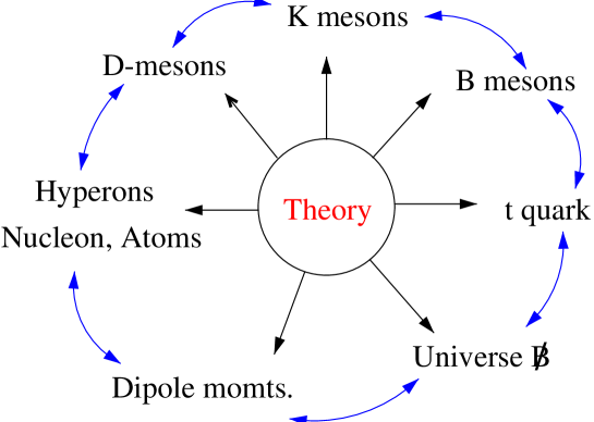
Figure 16: CP-Violation

In the standard model, all $CP$-violation resides in the CKM matrix which describes the couplings of the W-bosons to the quarks of different charges. Thus all appreciable $CP$-violation occurs within flavor physics. Thus, one obvious strategy to search for new forces and particles would be to look for non-zero $CP$-violating effects in electric dipole moments or asymmetries in nuclear reactions. Unfortunately, the effects of new physics are judged to be quite small (apart from the dipole moments). Therefore more chance is given to the flavor sector instead, that is the physics of Kaons and mostly B-mesons. For a recent extensive review of $CP$-violation, see ref. ([1]).

The unitarity of the CKM matrix

$$V=\left(\begin{array}[]{ccc}V_{ud}&V_{us}&V_{ub}\\ V_{cd}&V_{cs}&V_{cb}\\ V_{td}&V_{ts}&V_{tb}\end{array}\right)$$ (38)

implies among others the triangle relation

$$V_{ud}V_{ub}^{*}+V_{cd}V_{cb}^{*}+V_{td}V_{tb}^{*}=0$$ (39)

which relates observable products of matrix elements and gives stringent tests of the validity of the standard model. Using the Wolfenstein parameterization, and scaling as usual the bottom side to one, we can write for the other sides of the scaled triangle

$$R_{b}=\frac{1}{A\lambda^{3}}V_{ud}V_{ub}^{*}=\bar{\varrho}+i\bar{\eta}\qquad,\qquad R_{t}=\frac{1}{A\lambda^{3}}V_{td}V_{tb}^{*}=1-(\bar{\varrho}+i\bar{\eta}).$$ (40)

Here, following ref. [2], the quantities

$$\bar{\varrho}=\varrho(1-\frac{\lambda^{2}}{2})\,\,\,\bar{\eta}=\eta(1-\frac{\lambda^{2}}{2})$$ (41)

are introduced to take into account even higher powers of $\lambda$.

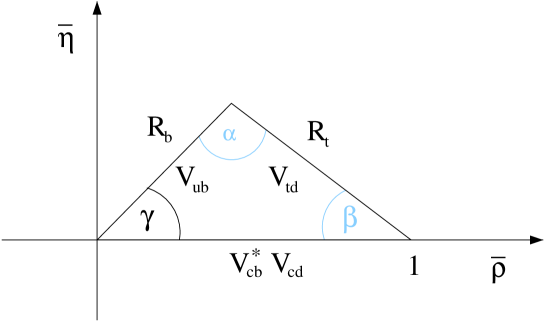
Figure 17: Unitarity triangle in the complex $(\bar{\varrho},\bar{\eta})$ plane.

An elaborate analysis of superallowed $\beta$ decay, semileptonic Kaon and $D$-meson decays and decays of $B$ mesons into charmed and charmless final states yields [3]

$$\begin{array}[]{cc}V_{ud}=0.9736\pm 0.001&V_{cs}=1.010\pm 0.16\\ V_{us}=0.2205\pm 0.0018&V_{cd}=0.224\pm 0.016\\ V_{ub}=0.04\pm 0.002&V_{cb}=0.0036\pm 0.006\\ \end{array}$$ (42)

These are (apart from corrections) all tree-level processes and therefore thought to be governed by the standard model . They are however not sufficient to check unitarity (unless very precise data from $t$ decays would be available, or if the sum of the squares would be significantly away from $1$).

Further input comes from loop-induced observables. They can be calculated within perturbation theory and input from hadronic physics. While the former are rather reliable and usually give results accurate to 10 percent or so, the latter are generally difficult to estimate. One usually considers the Kaon-mixing quantity $\epsilon_{K}$, the mass difference of the $B$ and the $\bar{B}$ mesons (and also of the $B_{s}$ and $\bar{B}_{s}$ mesons). This analysis has resulted in the range of values for the three angles $\alpha$, $\beta$ and $\gamma$ of the unitary triangle and its sides. The hadronic uncertainties are summarized in [4] and are reflected by

$$|R_{b}|=0.39\pm 0.07~{}~{}~{}~{}~{}~{}|R_{t}|=0.98+0.04-0.22$$ (43)

and by [5, 6, 7]

$$(\sin 2\beta)_{\rm SM}=0.75\pm 0.20.$$ (44)

The new results this summer concern the angle $\beta$. It was found that the coefficient a of $sin(\Delta M_{B_{d}})$ in the asymmetry for $B\to J/\Psi K_{S}$ is

$$a=0.79\pm 0.4(CDF)\cite[cite]{[\@@bibref{}{CDFB}{}{}]}$$ (45)

$$a=0.45\pm 0.4(Belle)\cite[cite]{[\@@bibref{}{Belle}{}{}]}$$ (46)

$$a=0.12\pm 0.4(BaBar)\cite[cite]{[\@@bibref{}{BaBar}{}{}]}$$ (47)

In the standard model, one has $a=sin(2\beta)$; comparing eqs. (44) and (10) we see a surprising inconsistency. Of course, this is a preliminary result, and may disappear as experiments collect more statistics. However, it makes it mandatory to investigate $CP$-violation in a (standard) model independent way. Unless $CP$-violation within the standard model is grossly wrong, this program essentially amounts to making many measurements and extracting discrepancies between quantities thought to be the same in the standard model. Many authors have discussed this situation; see e.g. [11, 12, 13, 14, 15].

3.3.2 A more general framework

New physics may affect every process. Because the standard model describes the most important weak decays, we will assume that it accounts for semileptonic and tree-level quark decays, at least to the required accuracy. This assumption can be tested, by investigating the consistency of different semileptonic decays, bounds from LEP etc. As an example consider the strengths of the effective Hamiltonians

$${\cal H}_{eff}=G_{F}(\bar{c}_{L}\gamma_{\mu}b_{L})(\bar{s}_{L}\gamma^{\mu}c_{L})$$ (48)

$${\cal H}_{eff}=G_{F}(\bar{u}_{L}\gamma_{\mu}b_{L})(\bar{s}_{L}\gamma^{\mu}u_{L}).$$ (49)

In the standard model, they are difficult to estimate. One usually considers the Kaon-mixing quantity $\epsilon_{K}$, the mass difference of the $B$ and the $\bar{B}$ mesons (and also of the $B_{s}$ and $\bar{B}_{s}$ mesons). On the other hand, a new neutral intermediate boson, say $Z^{\prime}$, may exist, coupled to the current $(\bar{s}_{L}\gamma_{\mu}b_{L})$. and $(\bar{c}_{L}\gamma_{\mu}c_{L})$. If it also couples to quark and lepton pairs, such as $(\bar{u}_{L}\gamma_{\mu}u_{L})$ and $(\bar{c}_{L}\gamma_{\mu}c_{L})$, it would contribute to the above interaction, to $B_{s}$ mixing, to $B_{s}\to l^{+}l^{-}$ etc. If the couplings are the same for all these pairs, the effective strength would be the same for the two terms in eqs. (48) and (12). Therefore a new $Z^{\prime}$-mediated interaction would induce a deviation from the standard model result that the couplings of the two interactions have a relative strength of $\lambda^{2}$. Thus detailed studies could in principle also test the first assumption. But of course, there are various experimental and theoretical difficulties to overcome before one will obtain accurate enough results.

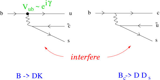
Figure 18: two quark diagrams whose interference gives $\gamma$

From fig. 3 we see that the determination of the angle $\gamma$ from tree level processes involves the interference of amplitudes proportional to $V_{ub}$ and $V_{ub}$ respectively. This is achieved in processes where the two diagrams of fig. 3 contribute. A well known example are the decays $B\to DK$ [16, 17]; more recently the advantage of $B_{c}\to DD_{s}$ was stressed [18]. The idea is the same as in the previous papers on $B\to DK$ : One needs to measure the six amplitudes shown in Fig. 4. One usually considers the Kaon-mixing quantity $\epsilon_{K}$, the mass difference of the $B$ and the $\bar{B}$ mesons (and also of the $B_{s}$ and $\bar{B}_{s}$ mesons). the sides of the triangles in Fig. 3 are of similar length and an extraction of $\gamma$ seems possible with the $10^{10}$ or so $B_{c}$-mesons expected at LHC. This method does not suffer from hadronic uncertainties.

Figure 19: The extraction of $\gamma$ from $B_{c}^{\pm}\to D^{\pm}_{s}\{D^{0},\overline{D^{0}},D^{0}_{+}\}$ decays.

The experimental difficulties associated with these decays have lead to other possibilities. The decays $B\to K\pi$ are sensitive to the interference of the tree level diagram (with $V_{ub}$) and the penguin diagram. This also yields the angle $\gamma$ if the penguin graph has no extra phase. This decay has been discussed by many people [19].

A third possibility that was discussed are the decays $B^{0}\to D^{\pm}\pi^{\mp}$ [20]. The usual mixing-decay formalism yields for the time dependent asymmetries the coefficients

$$a\sim Im(e^{-i(2\phi_{mix}+\gamma)})const$$ (50)

$$\bar{a}~{}\sim Im(e^{-i(2\phi_{mix}+\gamma)})/const.$$ (51)

where const is an unknown hadronic number. It cancels in the product which then yields the combination

$$2\phi_{mix}+\gamma$$ (52)

The $B\bar{B}$ mixing angle $\phi_{mix}$ can be determined as usual from the decay $B\to J/\Psi K_{s}$.

The other angles of the triangle cannot be determined by a tree level analysis independently. But we see, that the tree level analysis allows difficult to estimate. One usually considers the Kaon-mixing quantity $\epsilon_{K}$, the mass difference of the $B$ and the $\bar{B}$ mesons (and also of the $B_{s}$ and $\bar{B}_{s}$ mesons). to determine the unitary triangle of the standard model. It yields, in principle, also the unknown side $R_{t}$ and the angle $\beta$. Any further independent measurement of these quantities checks the standard model with high accuracy, but it requires loop effects.

3.3.3 New physics: phenomenology

Among the $CP$-violating observables, the mixing-decay asymmetry is the cleanest theoretically [21]. It is therefore reasonable to start an investigation of new physics with this quantity. Denoting the coefficient of $sin(\Delta mt)$ by $a$, one has in general

$$a_{M\to F}=Im((\frac{p}{q})_{M}\frac{a}{\bar{a}}(\frac{p}{q})_{F})$$ (53)

where ($\frac{p}{q}$) are the mixing parameters and $a$, $\bar{a}$ the amplitudes for $M\to F$ and $M\to\bar{F}$, respectively.

Setting for the $B$-meson mixing element $M_{12}$

$$M_{12}=r^{2}e^{2i\phi^{NP}}e^{2i\beta}|M_{12}^{SM}|$$ (54)

to account for a possible new phase and magnitude of the mixing, the asymmetry coefficient is given in the table below:

$quarks$	$B_{d}$	$a$	$B_{s}$	$a$
$b\to c\bar{c}s$	$\Psi K_{s}$	$\beta+\phi^{NP}_{d}$	$DD_{s}$	$\phi^{NP}_{s}$
$b\to s\bar{s}s$	$\Phi K_{s}$	$\beta+\phi^{NP}_{d}+\phi^{A}$	$\Phi\Phi$	$\phi^{NP}_{s}+\phi^{A}$
$b\to u\bar{u}s$	$\pi\pi$
$b\to c\bar{c}d$	$D^{+}D^{-}$
$b\to u\bar{u}s$	$\pi^{0}K_{s}$
$b\to s\bar{s}s$	$\Phi\pi$

The phase $\phi^{A}$ takes into account a possible new phase in the decay. The entries left out receive possibly sizeable contributions from penguin diagrams and cannot be brought to the simple form. This result tells us that comparing the different asymmetries, we can check the consistency of the standard model and determine the phases of new physics.

New physics will also influence other $CP$-violating observables, such as the direct asymmetries of, say charged B-meson decays. In cases such as $B\to K\pi$, where the asymmetry is small in the standard model new physics may give rise to sizeable asymmetries. Of course, one need to continue the search for these, but because of the difficulty of calculating direct asymmetries, only quantitative statements are possible.

3.3.4 New physics: analysis

If new physics is associated with a scale $\Lambda$ much above the weak scale ($\sim M_{W}$), the total Lagrangian density may be written in the form [22]

$${\cal L}={\cal L}^{SM}+\sum{d_{i}{\cal O}_{i}^{NP}}$$ (55)

where the $O_{i}$ are operators of dimension six induced by new physics and their coefficients $d_{i}$ are of order($1/{\Lambda^{2}}$). This ’effective’ Lagrangian is not renormalizable, and therefore one usually uses the new operators only at tree level (see a discussion by). The $CP$- violation induced by effective operators ${\cal O}_{i}^{N}P$ can in most cases only be seen when they are in loops, because the imaginary part (discontinuity) of the corresponding Feynman graph is responsible for $CP$-asymmetry. At low energies we then have an effective Hamiltonian

$${\cal H}=\sum{c_{i}{\cal O}_{i}^{SM}}+\sum{d_{i}{\cal O}_{i}^{NP}}$$ (56)

The amplitudes for a process $I\to F$ and the CP conjugated one $\bar{I}\to\bar{F}$ then are

$$A(I\to F)=\sum{c_{j}(R_{j}+iI_{j})^{SM}}+\sum{d_{j}^{*}(R_{j}+iI_{j})^{NP}}$$ (57)

where $R$ and $I$ are the dispersive and absorptive parts of the matrix elements. For the charge-conjugated process we have similarly

$$A(\bar{I}\to\bar{F})=\sum{c_{j}^{*}(R_{j}+iI_{j})^{SM}}+\sum{d_{j}(R_{j}+iI_{j})^{NP}}$$ (58)

When we calculate the $CP$-violating asymmetry $\alpha\sim(|A(I\to F)|^{2}-|A(\bar{I}\to\bar{F})|^{2})$, we obtain in leading order in QCD and in NP

$$\alpha\sim Im(cd^{*})(R^{SM}I^{NP}-R^{NP}I^{SM}).$$ (59)

$R^{NP}$ is a (finite) tree level amplitude, however also the loop $I^{NP}$ is finite. Therefore the problems associated with a the non-renormalizable theory $\sum{d_{i}{\cal O}_{i}^{NP}}$ disappear and exact predictions are indeed possible for the the $CP$-violating asymmetry. Therefore, an analysis of the effects of new operators is possible also at for CP-violating asymmetries, and not just at tree level!

3.3.5 New physics: models

Virtually any model beyond the standard one carries new sources for flavour and $CP$-violations. It is therefore more economical to look at them in increasing complexity.

The simplest one are the minimal flavour violating ones (MFV) where all sources of flavour violation reside in the CKM matrix. This results in many cases in a simple modification of the coefficients in the usual loop expressions. However, there still is a unitary triangle, but its sizes and angles may change. It was analyzed by Ali and London [6]; recently Buras and Buras [15] found a clever lower bound on $sin(2\beta)$. The idea is simple. For both $\epsilon$ and the $B$-meson mass difference, the standard model contribution consists mostly of a $W-W-t-t$ box diagram; its value might be denoted by $F_{tt}$. The $MFV$ modify this to

$$F_{tt}=S_{0}(m_{t})~{}(1+f)~{}.$$ (60)

Then we can write for $\epsilon_{K}$

$$\epsilon_{K}\sim\bar{\eta}\left[(1-\bar{\varrho})A^{2}\eta_{2}F_{tt}+P_{c}(\varepsilon)\right]A^{2}\hat{B}_{K}$$ (61)

while the $B$-meson mass difference yields the relation

$$R_{t}=1.26~{}\frac{R_{0}}{A}\frac{1}{\sqrt{F_{tt}}}~{},$$ (62)

where

$$R_{0}=\sqrt{\frac{(\Delta M)_{d}}{0.47/{\rm ps}}}\left[\frac{200~{}mev}{F_{B_{d}}\sqrt{\hat{B}_{d}}}\right]\sqrt{\frac{0.55}{\eta_{B}}}~{}.$$ (63)

With

$$\sin 2\beta=\frac{2\bar{\eta}(1-\bar{\varrho})}{R^{2}_{t}}$$ (64)

one gets [2]

$$\sin 2\beta=\frac{1.26}{R^{2}_{0}\eta_{2}}\left[\frac{0.226}{A^{2}\hat{B}_{K}}-\bar{\eta}P_{c}(\varepsilon)\right].$$ (65)

Since unitarity implies $\bar{\eta}\leq R_{b}~{}$, there exists a lower bound on $\sin 2\beta$. A careful numerical analysis implies

$$\bar{\eta}\geq 0.34.$$ (66)

The lower bound in fact corresponds to a $F_{tt}$ which is three times larger than the standard model value.

Supersymmetry is a attractive candidate for new physics. In general, there are many new $CP$-violating phases. Since they can directly affect observables such a the electric dipole moment, it is natural to take them to be small (approximate $CP$-violation, [1]). In this situation, also $CP$-violating effects in the $B$-system are small. This implies a small angle $\beta$. This is in contrast to the standard model, where the flavour structure suppresses CP-violation.

The problem with this scheme is that it is hard to get $\epsilon_{K}$ right and that $\epsilon^{\prime}/\epsilon$ tends to be to small.

Similarly, models with left-right symmetry tend to have small $CP$-violating phases, thus the effects tend to be small also.

3.3.6 $CP$-violation in $D$-mesons

In the standard model, $CP$-violation is small in the $D$-System. This is partly due to the rather large tree-level decay rates and small coupling of the third generation. Therefore one would expect new physics $CP$-violation mostly in the mixing (see [1] for a more detailed discussion). Recent studies of time-dependent decay rates of $D^{0}\rightarrow K^{+}\pi^{-}$ by the CLEO collaboration [23] and measurements of the combination of $D^{0}\rightarrow K^{+}K^{-}$ and $D^{0}\rightarrow K^{-}\pi^{+}$ rates by the FOCUS collaboration [24] gave first information on the mixing.

As usual, one define the mixing quantities

$$x\equiv{m_{2}-m_{1}\over\Gamma},\ \ \ y\equiv{\Gamma_{2}-\Gamma_{1}\over 2\Gamma}.$$ (67)

CP-violation in the mixing is defined by the angle $\phi$. The experiments find that the quantity $y\cos\phi$ is significantly larger than the expectation in the standard model. The errors being large, this result is not yet significant, but it shows the potential of $D$-meson physics.

3.3.7 $K$-physics

Finally let me mention $K$-physics. Of course, efforts continue in calculating $\epsilon^{\prime}/\epsilon$. However, the rare decays $K^{+}\to\pi^{+}\nu\bar{\nu}$ and $K^{0}\to\pi^{0}\nu\bar{\nu}$ provide a theoretically clean way to measure (in the standard model) $|V_{td}|$ and $ImV_{td}$ [25]. Clearly, this can be used as a test of the unitary triangle, however the measurement of the neutral decays is not easy and probably many years away.

3.3.8 Conclusions

The new results on $\sin 2\beta$ are surprising; they may indicate a failure of the standard model. Several parameters have to be stretched beyond their reasonable values to account for them. One can modify the standard model to accommodate the small value of $\sin 2\beta$, but it is not clear that these modifications are consistent.

Nevertheless, the result brings back the (old) view, that a (standard) model independent and broad analysis of $CP$-violation is required in order to fully understand this phenomenon and the need for new interaction. this implies in particular measurements of many decay channels.

I have sketched strategies to determine the source of $CP$-violation for the case that the standard model accounts for tree level processes and given a phenomenological framework to calculate the effects of new operators. Needless to say that all of this will take many years of hard work on both the experimental and the theoretical side and that also less perfect measurements have to be pursued.

References

4 What can we learn from $\epsilon^{\prime}/\epsilon$?

4.1 CP violation in the kaon system

V. Martin, University of Edinburgh

CP violation was first observed in the neutral kaon system by Christenson, Cronin, Fitch and Turlay in 1964  [1] when they observed the long-lived neutral kaon decay into a $\pi^{+}\pi^{-}$ state. To date, the neutral kaon system is the only place where CP violation has been conclusively observed.

In the neutral kaon system CP violation is classified into two types: indirect and direct, parameterised by $\epsilon$ and $\epsilon^{\prime}$ respectively. Indirect CP violation may be observed through the asymmetry in the mixing of the neutral kaons. Direct CP violation may be observed through the asymmetry in the decays of the neutral kaons. As direct CP violation is a much smaller effect than indirect CP violation, the ratio $\mathcal{R}e({\epsilon^{\prime}/\epsilon})\approx{\epsilon^{\prime}/\epsilon}$ is usually considered as the measurement of direct CP violation. The last generation of $\mathcal{R}e(\epsilon^{\prime}/\epsilon)$ experiments announced final results in 1993. The NA31 experiment at CERN had a result which was compatible with direct CP violation: $\mathcal{R}e(\epsilon^{\prime}/\epsilon)=(23.0\pm 6.5)\times 10^{-4}$ [2], whereas the E731 experiment at FNAL found a result compatible with no direct CP violation: $\mathcal{R}e(\epsilon^{\prime}/\epsilon)=(7.4\pm 5.9)\times 10^{-4}$ [3].

This disagreement prompted a new generation of direct CP violation experiments with the aim of measuring $\mathcal{R}e(\epsilon^{\prime}/\epsilon)$ at the $10^{-4}$ level.

Theoretical estimates for the value of $\mathcal{R}e(\epsilon^{\prime}/\epsilon)$ are based on QCD calculations. The short distance contributions have been reliably calculated using perturbative-QCD [4]. Various methods have been used to estimate the long distance effects, such as chiral perturbation theory and lattice QCD. Figure 20 shows some recent theoretical predictions of $\mathcal{R}e(\epsilon^{\prime}/\epsilon)$.

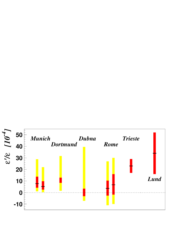
Figure 20: Recent theoretical estimates of $\mathcal{R}e(\epsilon^{\prime}/\epsilon)$ in chronological order [5, 6, 7, 8, 9]. The red/dark-grey error bars correspond to a Gaussian treatment of the input parameters. The yellow/light-grey error bars correspond to a flat scanning of all the input parameters. The cross lines corresponds to the most favoured value. Where there are two different results from one group, these correspond to different renormalisation schemes.

Experimentally, the parameter $\mathcal{R}e(\epsilon^{\prime}/\epsilon)$ is obtained by measuring the double ratio of decay rates ($\mathbf{R}$) of the long-lived and short-lived neutral kaons $\mathrm{K_{L}}$ and $\mathrm{K_{S}}$ into two pion final states:

$$\mathbf{R}\equiv\frac{\Gamma(\mathrm{K_{L}}\rightarrow\pi^{0}\pi^{0})/\Gamma(\mathrm{K_{S}}\rightarrow\pi^{0}\pi^{0})}{\Gamma(\mathrm{K_{L}}\rightarrow\pi^{+}\pi^{-})/\Gamma(\mathrm{K_{S}}\rightarrow\pi^{+}\pi^{-})}=1-6\,\mathcal{R}e(\epsilon^{\prime}/\epsilon)$$ (68)

Currently there are three dedicated experiments analysing or taking data with the aim of measuring $\mathcal{R}e(\epsilon^{\prime}/\epsilon)$: KTEV at FNAL, NA48 at CERN and KLOE at the DA$\Phi$NE $\Phi$ factory at Frascati. Each of these experiments was designed specifically to measure $\mathcal{R}e(\epsilon^{\prime}/\epsilon)$. In particular, they were designed to record high statistics and to minimise systematic errors in the measurement of $\mathcal{R}e(\epsilon^{\prime}/\epsilon)$. The following discussion here will focus on the measurements from NA48 and KTeV, which were presented at this workshop.

In the measurement of the double ratio R, many systematic effects cancel, such as the number of $\mathrm{K_{S}}$ and $\mathrm{K_{L}}$ particles produced, and the efficiency of detecting the charged and neutral final states.

The NA48 and KTeV experiments use a similar experimental set-up, aiming to exploit many of the cancellations in the measurement of $\mathbf{R}$. In order to be able to detect all four $\mathcal{R}e(\epsilon^{\prime}/\epsilon)$ decay modes simultaneously, both experiments employ a double beam technique: two neutral kaon beams are produced at different distances from the detector. Decays from the beam with the longer path length are predominantly $\mathrm{K_{L}}$ decays whereas decays from beam with the shorter path length are predominantly $\mathrm{K_{S}}$.

KTeV uses two identical, parallel, neutral kaon beams. A plastic scintillator regenerator is placed in one of the beams to regenerate $\mathrm{K_{S}}$ particles. The position of the decay products in the detectors can be used to determine whether the decay came from the vacuum or regenerator beam. The two NA48 beams are created by colliding the SPS protons on identical beryllium targets. The so-called $\mathrm{K_{L}}$ and $\mathrm{K_{S}}$ targets are placed respectively $240\;\mathrm{m}$ and $122\;\mathrm{m}$ upstream of the detector. The targets are arranged such that the two beams converge, meeting at the centre of the electromagnetic calorimeter. The times of the protons in transport to the $\mathrm{K_{S}}$ target are recorded by the proton tagging detector. The proton times can be compared offline to the time of the decay products in the detectors to determine which of the beams the decay came from.

To detect the decay products of the neutral kaons both the NA48 and KTeV experiments have: a magnetic spectrometer to detect charged tracks and reconstruct $\mathrm{K}\rightarrow\pi^{+}\pi^{-}$ decays; a high-resolution electromagnetic calorimeter to detect photons from $\pi^{0}\rightarrow 2\,\gamma$ decays and a muon detector to reject background from $\mathrm{K_{L}}\rightarrow\pi^{\pm}\mu^{\mp}\nu_{\mu}$ decays.

NA48 uses a quasi-homogeneous Liquid Krypton calorimeter which contains $9\;\mathrm{m^{3}}$ of liquid krypton kept at $121\;\mathrm{K}$. KTeV has a Cesium-Iodide crystal calorimeter, made of 3,100 blocks of pure Cesium-Iodide. The quality of these two calorimeters is reflected in the resolution in measuring reconstructed masses from the $\mathrm{K}\rightarrow\pi^{0}\pi^{0}\rightarrow 4\,\gamma$ decays. NA48 achieves a resolution on the reconstructed $\gamma\gamma$ mass of $1.1\;\mathrm{MeV/c^{2}}$, and KTeV achieves a resolution on the reconstructed kaon mass of $1.7-1.9\;\mathrm{MeV/c^{2}}$.

The analysis of the data from the $\mathcal{R}e(\epsilon^{\prime}/\epsilon)$ experiments is, in principle, straightforward. The number of events in each of the four decay modes in counted and a initial value of R is obtained. Corrections must be made to this value of R for backgrounds, trigger efficiencies, detector energy scale, beam scattering, accidental effects and detector acceptance. In addition both experiments make corrections for effects due to mis-identifying which of the beams the decay came from. Most of these corrections are small due to the cancellations present in R.

The largest potential correction to R is due to the differential acceptance of the four decay modes. To reduce this correction NA48 uses the technique of weighting the $\mathrm{K_{L}}$ events so that the decay distribution of weighted $\mathrm{K_{L}}$ events is the same as the (unweighted) $\mathrm{K_{S}}$ events. This reduces the correction to R due to the acceptance from around $13\%$ to around $3\times 10^{-3}$, but leads to a reduction of statistical precision of $35-40\%$. KTeV instead relies on a detailed Monte Carlo simulation of the experiment to calculate the acceptance. They calculate a correction to R of around $4\%$, which they measure with a precision of $13.4\times 10^{-3}$ [10].

KTeV collected data for the $\mathcal{R}e(\epsilon^{\prime}/\epsilon)$ measurement during 1996, 1997 and 1999. A preliminary result based on some of the data taken during 1996 and 1997 is described in [10]. The result of that analysis is $\mathcal{R}e(\epsilon^{\prime}/\epsilon)=\left(28.0\pm 3.0(\mathrm{stat})\pm 2.6(\mathrm{syst})\pm 1.0(\mathrm{MC\;stat})\right)\times 10^{-4}$.

NA48 has collected data for the $\mathcal{R}e(\epsilon^{\prime}/\epsilon)$ measurement in the years 1997–99 and will take more data in 2001. Preliminary results based on the data taken in 1997 and 1998 have been announced [11, 12]. The combined result from these data sets is: $\mathcal{R}e(\epsilon^{\prime}/\epsilon)=(14.0\pm 4.3)\times 10^{-4}$, where the statistical and systematic errors have been added in quadrature, and the small correlation between systematic effects has been taken into account. The error on this result is currently dominated by systematic effects, but as the systematic error includes some statistical component, the error will improve significantly when more data is analysed.

Table 11 shows the number decays in each $\mathcal{R}e(\epsilon^{\prime}/\epsilon)$ mode analyzed by NA48 (in 1998) and KTeV for these preliminary results.

Figure 21 shows the preliminary NA48 and KTeV results along with the results from E731 and NA31. A weighted average of these four results gives $\mathcal{R}e(\epsilon^{\prime}/\epsilon)_{\mathrm{global}}=(19.2\pm 2.5)\times 10^{-4}$ with a $\chi^{2}/\mathrm{ndf}=10.4/3$. The yellow/light-grey band on figure 21 shows the $\pm 1\sigma$ allowed region of this average. As the $\chi^{2}$ per degree of freedom on the average is larger than 1, the approach proposed by the PDG can be used to rescale the error by $(\chi^{2}/\mathrm{ndf})^{1/2}=1.8$, resulting in $\mathcal{R}e(\epsilon^{\prime}/\epsilon)_{\mathrm{global}}=(19.5\pm 4.6)\times 10^{-4}$.

experiment	$\mathrm{K_{L}}\rightarrow\pi^{0}\pi^{0}$	$\mathrm{K_{S}}\rightarrow\pi^{0}\pi^{0}$	$\mathrm{K_{L}}\rightarrow\pi^{+}\pi^{-}$	$\mathrm{K_{S}}\rightarrow\pi^{+}\pi^{-}$
NA48	$1.80\times 10^{6}$	$1.14\times 10^{6}$	$7.46\times 10^{6}$	$4.87\times 10^{6}$
KTeV	$0.86\times 10^{6}$	$1.42\times 10^{6}$	$2.61\times 10^{6}$	$4.51\times 10^{6}$

Table 11: Numbers of decays for each $\mathcal{R}e(\epsilon^{\prime}/\epsilon)$ decay mode collected by NA48 in 1998 and by KTeV for their preliminary result. The numbers have been corrected for background decays. The KTeV numbers actually refer to the numbers of decays counted from the vacuum beam ($\mathrm{K_{L}}$) and the regenerator beam ($\mathrm{K_{S}}$).

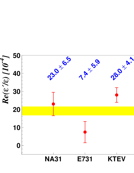
Figure 21: Recent measurements of $\mathcal{R}e(\epsilon^{\prime}/\epsilon)$ [2, 3, 10, 12]. Where both a statistical and systematic error is given, these have been added in quadrature. The yellow/light-grey band shows the $\pm 1\sigma$ allowed region of the average of these results.

The theoretical calculations shown in figure 20 generally predict smaller values for $\mathcal{R}e(\epsilon^{\prime}/\epsilon)$ than the experimental results, leading to some speculation that the measurement of $\mathcal{R}e(\epsilon^{\prime}/\epsilon)$ may be a sign of new physics. However due to the relatively large uncertainties reported by both theoretical calculations and experiments it is obviously too early to draw any conclusions on this issue.

Concluding on CP violation in kaon physics: the experimental picture is now much clearer than it was in 1993. Direct CP violation in the neutral kaon system is now firmly established. However, due to the large variation in the measurements, it is too early to settle on an exact value for $\mathcal{R}e(\epsilon^{\prime}/\epsilon)$. New, more precise experimental results will be produced by NA48, KTeV and KLOE in the future, allowing $\mathcal{R}e(\epsilon^{\prime}/\epsilon)$ to be known with an uncertainty of around $1\times 10^{-4}$.

References

4.2 Supersymmetry predictions for $\varepsilon^{\prime}/\varepsilon$

Shaaban Khalil, University of Sussex

4.2.1 Introduction

The most recent results of $\varepsilon^{\prime}/\varepsilon$ , which measures the size of the direct CP violation in $K_{L}\to\pi\pi$, reported by KTeV [1] and NA48 [2] lead to a world average of Re $\varepsilon^{\prime}/\varepsilon$ =$(21.4\pm 4.0)\times 10^{-4}$ [3]. This result is higher than the Standard Model (SM) predictions [4], opening the way to the interpretation that it may be a signal of new physics beyond the SM. The SM predictions for $\varepsilon^{\prime}/\varepsilon$ suffer from large theoretical uncertainties [5] such that one can not draw a definite conclusion if this observed high value of $\varepsilon^{\prime}/\varepsilon$ can be accommodated in the SM. In any case, one may wonder if the supersymmetry (SUSY) can be responsible for enhancing $\varepsilon^{\prime}/\varepsilon$ .

In the minimal supersymmetric extension of the SM (MSSM) there is no way of generating a sizable SUSY contribution to $\varepsilon^{\prime}/\varepsilon$ even if one assume that the SUSY CP violating phases are large and the electric dipole moments (EDM) of the electron and neutron are less than the experimental bounds due to the cancellation between the different contributions. This is mainly due to the assumption of universal boundary conditions of the soft-breaking terms [6, 7, 8, 9]. It has been shown that, without new flavor structure beyond the usual Yukawa couplings, general SUSY models with phases of the soft terms of order ${\cal O}(1)$ (but with a vanishing CKM phase $\delta_{\mathrm{CKM}}=0$) can not give a sizeable contribution to the CP violating processes [7, 8, 9, 10]. This means that the presence of non–universal soft breaking terms besides large SUSY phases is crucial to enhance these CP violation effects. In agreement with this, it has been explicitly shown that contributions to $\varepsilon_{K}$ are small within the dilaton–dominated SUSY breaking of the weakly coupled heterotic string model [10], where $A$–terms as well as gaugino masses are universal. On the other hand, it is well–known that the strict universality in the soft breaking sector is a strong assumption not realized in many supergravity and string inspired models [11, 12]. All these arguments indicate not only that the presence of non–universal soft terms can solve the problem of too large contributions to EDMs but also that it allows for large SUSY contributions in CP violation experiments. Hence, in this work we will follow this avenue and analyze the effects of non–universal soft terms in CP violation in the $K$–system [13, 14, 15].

4.2.2 CP violation in minimal supergravity model

It is well known that in SUSY models there are new possibilities for CP violation. In particular, the soft SUSY breaking terms contain several parameters that may be complex, as can also be the $\mu$-parameter. In the minimal supergravity model there are only two new CP-violating phases. This can be seen as follows. The parameters $M,A$ and $B$ and $\mu$ can be complex. But of these four phases only two are physical. First, by an R-rotation with R-charge $Q_{R}=1$ for lepton and quark superfields and $Q_{R}=0$ for the vector and the Higgs superfields, the gaugino mass parameter $M$ can be made real. Second, $B\mu$ can be made real by a change of phase of the Higgs superfield. This ensures that the Higgs vacuum expectation values are real. The remaining phases cannot be defined away and violate CP. One is in $A=A_{0}e^{i\phi_{A}}$ and the other in $B=B_{0}e^{i\phi_{B}}$. The $\mu$ parameter then has a fixed phase $\mu=\mu_{0}e^{-i\phi_{B}}$. In any phase convention

$$\phi_{A}=\mathrm{arg}(AM^{*}),\hskip 85.35826pt\phi_{B}=\mathrm{arg}(BM^{*}).$$ (69)

These phases can cause at one loop level an electric dipole moment (EDM) for the quarks and leptons, and therefore also for the neutron. It has been known for a long time that in the SUSY models the contributions to the neutron electric dipole moment are larger than the experimental limit $6.3\times 10^{-26}$ e cm unless either the new ‘SUSY phases’ are tuned to be of order $10^{-3}$, or the SUSY masses are of order a TeV. Such small phases can not generate sizable CP violation. Also they constitute a fine tuning. This is known as “ SUSY CP problem”. However, in the last few it has been suggested that a natural cancellation mechanism exists whereby the electric dipole moment of the neutron may be made small without such fine-tuning. In this case large SUSY phases are expected and still satisfy experimental bounds on the values of EDM of the electron and neutron.

In this section we will study the effect of these phases in CP violation observables as $\varepsilon$ and $\varepsilon^{\prime}/\varepsilon$ . We assume that $\delta_{CKM}=0$ to maximize this effect. The value of the indirect CP violation in the Kaon decays, $\varepsilon$, is defined as $\varepsilon=e^{i\frac{\pi}{4}}{\rm Im}M_{12}/\sqrt{2}\Delta m_{K},$ where $\Delta m_{K}=2{\rm Re}\langle K^{0}|H_{eff}|\bar{K}^{0}\rangle=3.52\times 10^{-15}$ GeV. The amplitude $M_{12}=\langle K^{0}|H_{eff}|\bar{K}^{0}\rangle$. The relevant supersymmetric contributions to $K^{0}-\bar{K}^{0}$ are the gluino and the chargino contributions, (i.e., the transition proceeds through box diagrams exchanging gluino-squarks and chargino-squarks). It is usually expected that the gluino is the dominant contribution. However, as we will show, it is impossible in the case of degenerate $A$-terms that the gluino gives any significant contribution to $\varepsilon$ when the CKM matrix is taken to be real even with large phase of $A$. The amplitude of the gluino contribution is given in terms of the mass insertion $\delta_{AB}$ defined by $\delta_{AB}=\Delta_{AB}/\tilde{m}^{2}$ where $\tilde{m}$ is an average sfermion mass and $\Delta$ is off-diagonal terms in the sfermion mass matrices. The mass insertion to accomplish the transition from $\tilde{d}_{iL}$ to $\tilde{d}_{jL}$ ($i,j$ are flavor indices) is given by

$$(\Delta^{d}_{LL})_{ij} \simeq -\frac{1}{8\pi^{2}}\left[\frac{K^{{\dagger}}(M_{u}^{diag})^{2}K}{v^{2}\sin^{2}\beta}\ln(\frac{M_{GUT}}{M_{W}})\right](3\tilde{m}^{2}+|X|^{2}),$$ (70)

$$(\Delta^{d}_{LR})_{ij} \simeq -\frac{1}{8\pi^{2}}\left[\frac{K^{{\dagger}}(M_{u}^{diag})^{2}K\ M_{d}}{v^{2}\sin^{2}\beta\cos\beta}\right]\ln(\frac{M_{GUT}}{M_{W}})X,$$ (71)

$$(\Delta^{d}_{RL})_{ij} \simeq -\frac{1}{8\pi^{2}}\left[\frac{M_{d}\ K^{{\dagger}}(M_{u}^{diag})^{2}K}{v^{2}\sin^{2}\beta\cos\beta}\right]\ln(\frac{M_{GUT}}{M_{W}})X,$$ (72)

$$(\Delta^{d}_{RR})_{ij} = 0,$$ (73)

where $X=A_{d}-\mu\ \tan\beta$. It is clear that $\Delta_{ij}$ in general are complex due to the complexity of the CKM matrix, the trilinear coupling $A$ and $\mu$ parameter. Here we assume the vanishing of $\delta_{CKM}$ to analyze the effect of the SUSY phases. We notice that $(\Delta^{d}_{LL})_{12}$ is proportional to $|X|^{2}$ i.e., it is real and does not contribute to $\varepsilon$ whatever the phase of $A$ is. Moreover, the values of the $(\Delta^{d}_{LR})_{12}$ and $(\Delta^{d}_{RL})_{12}$ are proportional to $m_{s}$ and $m_{d}$, hence they are quite small. Indeed in this case we find the gluino contribution to $\varepsilon$ is of order $10^{-6}$.

For the chargino contribution the amplitude is given by [16]

$$\langle K^{0}|H_{eff}|\bar{K}^{0}\rangle = -\frac{\displaystyle{G_{F}^{2}M_{W}^{2}}}{\displaystyle{(2\pi)^{2}}}(V_{td}^{*}V_{ts})^{2}f_{K}^{2}M_{k}\biggl{[}\frac{1}{3}C_{1}(\mu)B_{1}(\mu)$$ (74)

$$+ \bigl{(}\frac{M_{k}}{m_{s}(\mu)+m_{d}(\mu)}\bigr{)}^{2}\bigl{(}-\frac{5}{24}C_{2}(\mu)B_{2}(\mu)+\frac{1}{24}C_{3}(\mu)B_{3}(\mu)\bigr{)}\biggr{]}.$$

The complete expression for these function can be found in Ref. [16]. For low and moderate values of $\tan\beta$ the value of $C_{3}$ is much smaller than $C_{1}$ since it is suppressed by the ratio of $m_{s}$ to $M_{W}$. However, by neglecting the flavor mixing in the squark mass matrix $C_{1}$ turned out to be exactly real [9]. The imaginary part of $C_{1}$ is associated to the size of the intergenerational sfermion mixings, thus it is maximal for large $\tan\beta$. In low $\tan\beta$ case, that we consider, the imaginary part of $C_{1}$ is very small, and the gluino contribution is still the dominant contribution $\varepsilon$. In particular, we found that $\varepsilon$ is of order $10^{-6}$, which is less than the experimental value $2.26\times 10^{-3}$.

Now we consider the effect of these two phases ($\phi_{A}$ and $\phi_{\mu}$) on the direct CP violation parameter $\varepsilon^{\prime}/\varepsilon$ . Similar to the case of indirect CP violation parameter $\varepsilon$ , in the gluino contribution the $L$–$L$ transitions are almost real and the $L$–$R$ transitions are suppressed by two up Yukawa couplings and a down quark mass. Moreover, the analysis of chargino contribution is also the same as in the indirect CP violation. Even the experimental bounds on the branching ratio of $b\to s\gamma$ decay impose sever constraint on the LR transition. Therefore we do not find any significant SUSY CP violation effect in $\varepsilon^{\prime}/\varepsilon$ too.

4.2.3 Non–universal soft terms and SUSY CP violation

In the previous section, we have shown that CP violation effects are always very small in SUSY models with universal soft SUSY breaking terms. Recently, it has been shown that the non–universality of $A$–terms is very effective to generate large CP violation effects [7, 8, 13, 14, 17, 18]. In fact, the presence of non–degenerate $A$–terms is essential for enhancing the gluino contributions to $\varepsilon^{\prime}/\varepsilon$ through large imaginary parts of the $L$–$R$ mass insertions, $\mathrm{Im}(\delta_{LR})_{12}$ and $\mathrm{Im}(\delta_{RL})_{12}$. These SUSY contributions can, indeed, account for a sizeable part of the recently measured experimental value of $\varepsilon^{\prime}/\varepsilon$ [1, 2]. In the following, we will present an explicit realization of such mechanism in the framework of a type I superstring inspired SUSY model. Within this model, it is possible to obtain non–universal soft breaking terms, i.e. scalar masses, gaugino masses and trilinear couplings.

Type I string models contain nine–branes and three types of five–branes ($5_{a}$, $a=1,2,3$). If we assume that the gauge group $SU(3)\times U(1)$ is on one of the branes (9–brane) and the gauge group $SU(2)$ is on another brane ($5_{1}$–brane). Chiral matter fields correspond to open strings spanning between branes. Thus, they have non–vanishing quantum numbers only for the gauge groups corresponding to the branes between which the open string spans. For example, the chiral field corresponding to the open string between the $SU(3)$ and $SU(2)$ branes can have non–trivial representations under both $SU(3)$ and $SU(2)$, while the chiral field corresponding to the open string, which starts and ends on the $SU(3)$–brane, should be an $SU(2)$–singlet. There is only one type of the open string which spans between the 9 and $5_{1}$–branes, which we denote it as $C^{95_{1}}$. However, there are three types of open strings which could start and end on the 9–brane, that is, the $C^{9}_{i}$ sectors (i=1,2,3), which corresponding to the $i$-th complex compact dimension among the three complex dimensions. If we assign the three families to the different $C^{9}_{i}$ sectors we obtain non–universality in the right–handed sector. In particular, we assign the $C^{9}_{1}$ sector to the third family and $C^{9}_{3}$ and $C^{9}_{2}$ to the first and second families respectively. Under these assumption the soft SUSY breaking terms are obtained, following the formulae in Ref. [11, 12]. The gaugino masses are obtained

$$M_{3} = M_{1}=\sqrt{3}m_{3/2}\sin\theta\ e^{-i\alpha_{S}},$$ (75)

$$M_{2} = \sqrt{3}m_{3/2}\cos\theta\ \Theta_{1}e^{-i\alpha_{1}}.$$ (76)

While the $A$-terms are obtained as

$$A_{C_{1}^{9}}=-\sqrt{3}m_{3/2}\sin\theta\ e^{-i\alpha_{S}}=-M_{3},$$ (77)

for the coupling including $C_{1}^{9}$, i.e. the third family,

$$A_{C_{2}^{9}}=-\sqrt{3}m_{3/2}(\sin\theta\ e^{-i\alpha_{S}}+\cos\theta\ (\Theta_{1}e^{-i\alpha_{1}}-\Theta_{2}e^{-i\alpha_{2}})),$$ (78)

for the coupling including $C_{2}^{9}$, i.e. the second family and

$$A_{C_{3}^{9}}=-\sqrt{3}m_{3/2}(\sin\theta\ e^{-i\alpha_{S}}+\cos\theta\ (\Theta_{1}e^{-i\alpha_{1}}-\Theta_{3}e^{-i\alpha_{3}})),$$ (79)

for the coupling including $C_{3}^{9}$, i.e. the first family. Here $m_{3/2}$ is the gravitino mass, $\alpha_{S}$ and $\alpha_{i}$ are the CP phases of the F-terms of the dilaton field $S$ and the three moduli fields $T_{i}$, and $\theta$ and $\Theta_{i}$ are goldstino angles, and we have the constraint, $\sum\Theta_{i}^{2}=1$. Thus, if quark fields correspond to different $C_{i}^{9}$ sectors, we have non–universal A–terms. Then we obtain the following A–matrix for both of the up and down sectors,

$$A=\left(\begin{array}[]{ccc}A_{C^{9}_{3}}&A_{C^{9}_{2}}&A_{C^{9}_{1}}\\ A_{C^{9}_{3}}&A_{C^{9}_{2}}&A_{C^{9}_{1}}\\ A_{C^{9}_{3}}&A_{C^{9}_{2}}&A_{C^{9}_{1}}\end{array}\right).$$ (83)

Note that the non–universality appears only for the right–handed sector. The trilinear SUSY breaking matrix, $(Y^{A})_{ij}=(Y)_{ij}(A)_{ij}$, itself is obtained

$$Y^{A}=\left(\begin{array}[]{ccc}&&\\ &Y_{ij}&\\ &&\end{array}\right)\cdot\left(\begin{array}[]{ccc}A_{C^{9}_{3}}&0&0\\ 0&A_{C^{9}_{2}}&0\\ 0&0&A_{C^{9}_{1}}\end{array}\right),$$ (84)

in matrix notation. In addition, soft scalar masses for quark doublets and the Higgs fields are obtained,

$$m_{C^{95_{1}}}^{2}=m_{3/2}^{2}(1-\frac{\displaystyle{3}}{\displaystyle{2}}\cos^{2}\theta\ (1-\Theta_{1}^{2})).$$ (85)

The soft scalar masses for quark singlets are obtained as

$$m_{C_{i}^{9}}^{2}=m_{3/2}^{2}(1-3\cos^{2}\theta\ \Theta^{2}_{i}),$$ (86)

if it corresponds to the $C_{i}^{9}$ sector.

In models with non-degenerate $A$–terms we have to fix the Yukawa matrices to completely specify the model. In fact, with universal $A$–terms the textures of the Yukawa matrices at GUT scale affect the physics at EW scale only through the quark masses and usual CKM matrix, since the extra parameters contained in the Yukawa matrices can be eliminated by unitary fields transformations. This is no longer true with non-degenerate $A$–terms. Here, we choose our Yukawa texture to be

$$Y^{u}=\frac{1}{v\cos{\beta}}{\rm diag}\left(m_{u},m_{c},m_{t}\right)~{},~{}~{}Y^{d}=\frac{1}{v\sin{\beta}}K^{\dagger}\cdot{\rm diag}\left(m_{d},m_{s},m_{b}\right)\cdot K$$ (87)

where $K$ is the CKM matrix. In this case one find that the mass insertion $\delta^{d}_{LR}$ can be written as [14]

$$(\delta_{LR}^{(d)})_{ij} = \frac{1}{m^{2}_{\tilde{q}}}\ m_{i}\ \Big{(}\delta_{ij}\ (c_{A}A_{C^{9}_{3}}^{*}\ +\ c_{\tilde{g}}\ m_{\tilde{g}}^{*}-\ \mu e^{i\varphi_{\mu}}\tan\beta)$$ (88)

$$+ K_{i2}\ K^{*}_{j2}\ c_{A}\ (A_{C^{9}_{2}}^{*}-A_{C^{9}_{3}}^{*})+K_{i3}\ K^{*}_{j3}\ c_{A}\ (A_{C^{9}_{1}}^{*}-A_{C^{9}_{3}}^{*})\Big{)}$$

where $m^{2}_{\tilde{q}}$ is an average squark mass and $m_{i}$ the quark mass. This expression shows the main effects of the non–universal $A$–terms. In the first place, we can see that the diagonal elements are still very similar to the universal $A$–terms situation. Apart of the usual scaling with the quark mass, these flavor–diagonal mass insertions receive dominant contributions from the corresponding $A_{C^{9}_{i}}$ terms plus an approximately equal contribution from gluino to all three generations and an identical $\mu$ term contribution. Hence, given that the gluino RG effects are dominant, also the phases of these terms tend to align with the gluino phase, as in the minimal supergravity. Therefore, EDM bounds constrain mainly the relative phase between $\mu$ and gluino (or chargino) and give a relatively weaker constraint to the relative phase between $A_{C^{9}_{3}}$ (the first generation $A$–term) and the relevant gaugino. Effects of different $A_{C^{9}_{i}}$ in these elements are suppressed by squared CKM mixing angles. However, flavor–off–diagonal elements are completely new in this model. They do not receive significant contributions from gluino nor from $\mu$ and so their phases are still determined by the $A_{C^{9}_{i}}$ phases and, in principle, they do not directly contribute to EDMs .

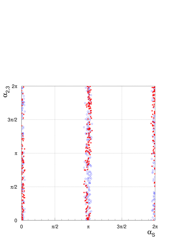
Figure 22: Allowed values for $\alpha_{2}$–$\alpha_{S}$ (open blue circles) and $\alpha_{3}$–$\alpha_{S}$ (red stars)

In figure 22 we show the allowed values for $\alpha_{S}$, $\alpha_{2}$ and $\alpha_{3}$ assuming $\alpha_{1}=\varphi_{\mu}=0$. We have imposed the EDM, $\varepsilon$ and $b\to s\gamma$ bounds with the usual bounds on SUSY masses. We can see that, similarly to the minimal supergravity, $\varphi_{\mu}$ is constrained to be very close to the gluino and chargino phases (in the plot $\alpha_{S}\simeq 0,\pi$), but $\alpha_{2}$ and $\alpha_{3}$ are completely unconstrained.

Finally, in figure 23 we show the values of $Im(\delta^{(d)}_{LR})_{21}$ versus the gluino mass in the same regions of parameter space and with the same constraints as in figure 22. As we can see due to the effect of the off-diagonal phases a large percentage of points are above or close to $1\times 10^{-5}$, hence, sizeable supersymmetric contribution to $\varepsilon^{\prime}/\varepsilon$ can be expected in the presence of non-universal $A$–terms.

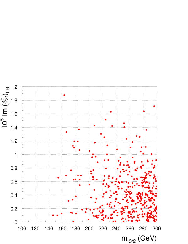
Figure 23: $(\delta_{LR}^{(d)})_{21}$ versus $m_{\tilde{g}}$ for experimentally allowed regions of the SUSY parameter space

4.2.4 Conclusions

Non–universal Supersymmetry soft breaking terms are a natural consequence in many supergravity or string inspired SUSY models. Moreover, the non–universality of the $A$–terms has a significant effect in the CP violation. We have shown that in these models a sizeable supersymmetric contribution to CP observables $\varepsilon^{\prime}/\varepsilon$ and $\varepsilon$ can be easily obtained.

References

5 $B_{s}\to J/\psi\phi$ for $\delta\gamma$ and the width difference in the $B_{d}$ - $\overline{B}_{d}$  system

5.1 The decays $B_{s}\to J/\psi\eta$ vs. $B_{s}\to J/\psi\phi$ for $\delta\gamma$

Amol S. Dighe, CERN

5.1.1 Disentangling the CP eigenstates

The decay rate of the mode $B_{s}\to J/\psi\eta$ as a function of time is approximately given as

$$\frac{d\Gamma(B_{s}\to J/\psi\eta)}{dt}\approx|{\cal A}(0)|^{2}~{}\left[e^{-\Gamma_{L}t}+2e^{-\bar{\Gamma}t}\sin(\Delta m_{s}t)\delta\gamma\right]~{}~{},$$ (89)

where $\bar{\Gamma}\equiv(\Gamma_{L}+\Gamma_{H})/2$. The non-oscillatory part of (89) gives the value of $\Gamma_{L}$ whereas the oscillatory part gives $\delta\gamma$.

The decay mode $B_{s}\to J/\psi(\ell^{+}\ell^{-})\phi(K^{+}K^{-})$ is another candidate for the determination of $\delta\gamma$. It has the advantages of having a larger branching ratio and a higher efficiency of detection (since all the four final state particles are charged). However, the final state $J/\psi\phi$ is not a pure $CP$ eigenstate, but an admixture of $CP$ odd and $CP$ even components. Here, we argue that in spite of this, the mode $J/\psi\phi$ is a better candidate than $J/\psi\eta$ for determining $\delta\gamma$.

The most general amplitude for this decay can be written in terms of the polarizations $\epsilon_{J/\psi},\epsilon_{\phi}$ of the two vector mesons as [1, 2]:

$$A(B_{s}\to J/\psi\phi)=A_{0}\left(\frac{m_{\phi}}{E_{\phi}}\right)\epsilon^{*L}_{J/\psi}\epsilon^{*L}_{\phi}-\frac{A_{\parallel}}{\sqrt{2}}~{}\epsilon^{*T}_{J/\psi}\cdot\epsilon^{*T}_{\phi}-i\frac{A_{\perp}}{\sqrt{2}}~{}\epsilon^{*}_{J/\psi}\times\epsilon^{*}_{\phi}\cdot{\bf\hat{p}}~{}~{},$$ (90)

where $E_{\phi}$ is the energy of $\phi$ and ${\bf\hat{p}}$ is the unit vector in the direction of $\phi$ in the $J/\psi$ rest frame. The superscripts $L$ and $T$ represent the longitudinal and transverse components respectively. Since the direct $CP$ violation in this mode is negligible, the amplitudes $A_{0}$ and $A_{\parallel}$ are $CP$ even whereas $A_{\perp}$ is $CP$ odd.

The final states with different $CP$ parities can be separated through their different angular distributions. The decay $B_{s}\to J/\psi(\ell^{+}\ell^{-})\phi(K^{+}K^{-})$, however, has four final state particles, which implies that the angular distributions will, in general, be in terms of three physical angles [1, 2]. Such a three angle analysis has been performed [3], where preliminary studies indicate that that the values of $\delta\gamma$ as low as 0.03 may be accessible, depending on the value of $x_{s}\equiv\Delta m_{s}/\bar{\Gamma}$.

However, more the number of angular terms, more formidable the task of disentangling their coefficients, which are the physical quantities of interest. The method of angular moments [2, 4] may be of some help, but with as many as 6 angular terms in the complete three angle distribution, the errors in the determination of the coefficients are large. Moreover, it involves a fit to as many as 8 independent parameters, some of which seem to have strong correlations. Getting rid of these problems would increase the sensitivity on the value of $\delta\gamma$, and might bring its SM value within the domain of measurability.

The angular analysis can be simplified a lot if the angles are chosen such that the angular distribution that separates the $CP$ odd and even terms can be written in terms of a single angle. Here we show that such a angle may be defined for this decay. It follows on the lines of the arguments given in [5]. The transversity angle distribution reduces the problem to disentangling only two angular terms (as opposed to six earlier) and only five independent parameters (as opposed to eight).

5.1.2 The transversity angle

In the rest frame of $\phi$, the decay $B\to J/\psi K^{+}K^{-}$ is planar. Let us define the transversity axis as the one perpendicular to this decay plane. Let the decay plane be the $x-y$ plane, so that the $z$ axis is the transversity axis. The transversity angle is the angle made by the spin of $J/\psi$ with this axis.

The final state $\{J/\psi K^{+}K^{-}\}$ in the rest frame of $\phi$ may be represented in the basis of $|\vec{p}_{K^{+}}\vec{p}_{K^{-}}\vec{p}_{\psi}J_{z\psi}\rangle_{\phi}$, where $J_{z\psi}$ is the $z$ component of the spin of $J/\psi$. Clearly, $\vec{p}_{K^{+}}=-\vec{p}_{K^{-}}$. Consider the operator ${\cal R}_{CP}$, which combines charge conjugation with the reflection in the $x-y$ plane:

$${\cal R}_{CP}\equiv{\cal C}{\cal R}_{P}={\cal CP}e^{i\pi J_{z}}~{}~{}$$ (91)

where ${\cal C}$ and ${\cal P}$ are the charge conjugation and parity transformation operators respectively. Since the total angular momentum of the final state is zero, from (91), we have

$${\cal R}_{CP}|\vec{p}_{K^{+}}\vec{p}_{K^{-}}\vec{p}_{\psi}J_{z\psi}\rangle_{\phi}=(CP)_{f}|\vec{p}_{K^{+}}\vec{p}_{K^{-}}\vec{p}_{\psi}J_{z\psi}\rangle_{\phi}~{}~{},$$ (92)

where $(CP)_{f}$ is the $CP$ parity of the final state.

On the other hand, both $|\vec{p}_{K^{+}}\vec{p}_{K^{-}}\rangle_{\phi}$ and $|\vec{p}_{\psi}J_{z\psi}\rangle_{\phi}$ are separately eigenstates of ${\cal R}_{CP}$, and ${\cal R}_{CP}$ commutes with any boost in the decay plane. Then, if we denote the boost from $\phi$ rest frame to $J/\psi$ rest frame by ${\cal B}$, so that ${\cal B}|\vec{p}_{\psi}J_{z\psi}\rangle_{\phi}=|\vec{p}_{\psi}J_{z\psi}\rangle_{J/\psi}$, then

$${\cal R}_{CP}|\vec{p}_{K^{+}}\vec{p}_{K^{-}}\vec{p}_{\psi}J_{z\psi}\rangle_{\phi} = {\cal R}_{CP}|\vec{p}_{K^{+}}\vec{p}_{K^{-}}\rangle_{\phi}~{}{\cal B}^{-1}{\cal R}_{CP}{\cal B}|\vec{p}_{\psi}J_{z\psi}\rangle_{\phi}$$ (93)

$$= (CP)_{\phi}|\vec{p}_{K^{+}}\vec{p}_{K^{-}}\rangle_{\phi}~{}{\cal B}^{-1}(CP)_{J/\psi}e^{i\pi\tau}|\vec{p}_{\psi}J_{z\psi}\rangle_{J/\psi}~{},$$ (94)

where $\tau$ is the transversity of $J/\psi$, i.e. the projection of its spin along the transversity axis. Using $(CP)_{\phi}=(CP)_{J/\psi}=+1$ and the fact that ${\cal B}$ commutes with the other operators, we can write

$${\cal R}_{CP}|\vec{p}_{K^{+}}\vec{p}_{K^{-}}\vec{p}_{\psi}J_{z\psi}\rangle_{\phi} = |\vec{p}_{K^{+}}\vec{p}_{K^{-}}\rangle_{\phi}~{}e^{i\pi\tau}|\vec{p}_{\psi}J_{z\psi}\rangle_{\phi}$$ (95)

$$= (-1)^{\tau}~{}|\vec{p}_{K^{+}}\vec{p}_{K^{-}}\vec{p}_{\psi}J_{z\psi}\rangle_{\phi}~{}~{}.$$ (96)

From (92) and (96), we get

$$(CP)_{f}|\vec{p}_{K^{+}}\vec{p}_{K^{-}}\vec{p}_{\psi}J_{z\psi}\rangle_{\phi}=(-1)^{\tau}~{}|\vec{p}_{K^{+}}\vec{p}_{K^{-}}\vec{p}_{\psi}J_{z\psi}\rangle_{\phi}~{}~{},$$ (97)

which shows that the final states with even and odd $CP$ parities correspond to the states with the transversity of $J/\psi$ equal to 0 and $\pm 1$ respectively. There two states can easily be separated by using the parity conserving decay $J/\psi\to\ell^{+}\ell^{-}$ as an analyzer, and studying the angular distribution in the transversity angle, the angle made by the decay products with the transversity axis in the rest frame of $J/\psi$.

The above argument may be generalized and shown to be applicable in the case of all decays of the form $B\to AC(\to C_{1}C_{2})$, where (a) $A$ and $C$ are self-conjugate particles with $C_{1}$ and $C_{2}$ spinless and charge conjugates of each other (as in the case under discussion), (b) $A,C_{1},C_{2}$ all are self-conjugate particles, or (c) $A$ and $C$ are charge conjugates of each other, with $C_{1}$ and $C_{2}$ spinless particles. In all such cases, a transversity angle can be defined such that the angular distribution separates $CP$ odd and even final states [5].

5.1.3 Transversity angle distribution in $J/\psi\phi$

Let us define the angles as shown in Fig. 24. Let $x$ axis be the direction of $\phi$ in the $J/\psi$ rest frame, and let $z$ axis be perpendicular to the decay plane of $\phi\to K^{+}K^{-}$, with positive $y$ direction chosen such that $p_{y}(K^{+})\geq 0$. Then we define $(\theta,\varphi)$ as the decay direction of $l^{+}$ in $J/\psi$ rest frame and $\psi$ as the angle made by $K^{+}$ with $x$ axis in $\phi$ rest frame.

Figure 24: The definitions of angles $\theta,\varphi,\psi$. Here $\theta$ is the transversity angle.

The angular distribution is then given by

$$\frac{d\Gamma[B_{s}\to J/\psi\phi]}{d\cos\theta dt}\approx\frac{3}{8}|{\cal A}_{+}(t)|^{2}(1+\cos^{2}\theta)+\frac{3}{4}|{\cal A}_{-}(t)|^{2}\sin^{2}\theta~{}~{},$$ (98)

where $|{\cal A}_{+}(t)|^{2}\equiv|A_{0}(t)|^{2}+|A_{\parallel}(t)|^{2}$ and $|{\cal A}_{-}(t)|^{2}\equiv|A_{\perp}(t)|^{2}$ are the $CP$ even and $CP$ odd components respectively. The time evolution of these components is given by

$$|{\cal A}_{+}(t)|^{2} =|{\cal A}_{+}(0)|^{2}\times$$ (99)

$$\left[\cos^{2}(\delta\gamma)e^{-\Gamma_{L}t}+\sin^{2}(\delta\gamma)e^{-\Gamma_{H}t}+e^{-\bar{\Gamma}t}\sin(\Delta m_{s}t)\sin(2\delta\gamma)\right],$$

$$|{\cal A}_{-}(t)|^{2} =|{\cal A}_{-}(0)|^{2}\times$$ (100)

$$\left[\sin^{2}(\delta\gamma)e^{-\Gamma_{L}t}+\cos^{2}(\delta\gamma)e^{-\Gamma_{H}t}-e^{-\bar{\Gamma}t}\sin(\Delta m_{s}t)\sin(2\delta\gamma)\right].$$

The time evolution of either one (or both of) the components lets us determine the values of $\Gamma_{H},\Gamma_{L}$ and $\delta\gamma$.

The value of $\delta\gamma$ is small ($\approx 0.015$) in the standard model. To first order in $\delta\gamma$, eqs. (99) and (100) may be written as

$$|{\cal A}_{+}(t)|^{2} \approx |{\cal A}_{+}(0)|^{2}~{}\left[e^{-\Gamma_{L}t}+2e^{-\bar{\Gamma}t}\sin(\Delta m_{s}t)\delta\gamma\right]~{}~{},$$ (101)

$$|{\cal A}_{-}(t)|^{2} \approx |{\cal A}_{-}(0)|^{2}~{}\left[e^{-\Gamma_{H}t}-2e^{-\bar{\Gamma}t}\sin(\Delta m_{s}t)\delta\gamma\right]~{}~{}.$$ (102)

The time evolution (101) is exactly the one used for the determination of $\delta\gamma$ through $J/\psi\eta$ in (89). Since only two angular terms are present in (98), the separation of their coefficients is not hard. Therefore, the accuracy obtained through these two modes would be similar if the number of events were the same. However, the mode $J/\psi\phi$ is expected to have almost an order of magnitude more number of events than $J/\psi\eta$.

An interesting situation arises when the measured value of $\delta\gamma$ is large. This is clearly a signal of physics beyond the SM, in particular of an extra phase appearing in the $B_{s}-\bar{B}_{s}$ mixing. Using the exact expressions for time evolution (eqs. 99 and 100) will give a measurement of this physically interesting phase, whereas The approximate time evolution (eqs. 89, 101 and 102) will fail to do so. In this case, any advantage $J/\psi\eta$ would have had due to its being close to a $CP$ eigenstate is lost. The non-oscillatory part of (89) can no longer be used to give a clean measurement of $\Gamma_{L}$, since the time evolution now consists of two exponential decays with similar lifetimes. In [4], the information content per event in such decays has been quantified, and it has been shown that the mode with angular information may have orders of magnitude more information per event than the mode with time information alone. Adding this to the larger number of expected events in $J/\psi\phi$, the case for this mode becomes even stronger.

References

5.2 Width Difference in the $B_{d}$ - $\overline{B}_{d}$  system

A. Dighe, CERN, T. Hurth, CERN, C.S. Kim, Yonsei University

Within the standard model, the difference in lifetimes of $B_{d}$ mesons is CKM suppressed compared with the ones of $B_{s}$ mesons. A rough estimate leads to:

$$\frac{\Delta\Gamma_{d}}{\Gamma_{d}}\approx\frac{\Delta\Gamma_{s}}{\Gamma_{s}}\left|\frac{V_{cs}}{V_{cd}}\right|^{2}\approx 0.5\%~{}~{},$$ (103)

where $\Gamma_{d}$ is the average lifetime of the light and heavy $B_{d}$ mesons ($B_{d}^{L}$ and $B_{d}^{H}$ respectively). We denote these lifetimes by $\Gamma^{d}_{L},\Gamma^{d}_{H}$ respectively, and define $\Delta\Gamma_{d}\equiv\Gamma^{d}_{L}-\Gamma^{d}_{H}$.

More precisely, we get for $\Gamma_{12}$ at leading order using the standard notations [1, 2]

$$\Gamma_{12}={\displaystyle{-\frac{G_{F}^{2}m_{b}^{2}m_{B}}{24\pi}[\frac{5}{3}\frac{m_{B}^{2}}{(m_{b}+m_{d})^{2}}(K_{2}-K_{1})f_{B}^{2}B_{S}(V_{tb}V_{td}^{*})^{2}}}$$

$${\displaystyle{+\frac{8}{3}(K_{1}+\frac{K_{2}}{2})f_{B}^{2}B_{B}(V_{tb}V_{td}^{*})^{2}+8(K_{1}+K_{2})f_{B}^{2}B_{B}\frac{m_{c}^{2}}{m_{b}^{2}}V_{cb}V_{cd}^{*}V_{tb}V_{td}^{*}}}].$$ (104)

$K_{1}=-0.39$ and $K_{2}=1.25$ are combinations of Wilson coefficients. $B_{S}$ and $B_{B}$ are the bag factors corresponding to the matrix elements of the operators $Q_{S}\equiv(\bar{b}d)_{S-P}(\bar{b}d)_{S-P}$ and $Q\equiv(\bar{b}d)_{V-A}(\bar{b}d)_{V-A}$. Using the known expression for $M_{12}$ (see i.e. [1]) and $m_{b}=4.5$ GeV, we have

$$\frac{\Gamma_{12}^{0}}{M_{12}^{0}}=-5.0\times 10^{-3}\left(1.4\frac{B_{S}}{B_{B}}+0.24+2.5\frac{m_{c}^{2}}{m_{b}^{2}}\frac{V_{cb}V_{cd}^{*}}{V_{tb}V_{td}^{*}}\right).$$ (105)

In the vacuum saturation approximation one has $B_{S}/B_{B}=1$ at some typical hadronic scale.

With ${\rm Re}(\Gamma_{12}/M_{12})\simeq\Delta\Gamma/\Delta m$, and the measured value $x_{d}=\Delta m_{d}/\Gamma_{d}=0.73\pm 0.05$ we confirm the rough estimate (103) taking into account the large hadronic uncertaintities.

No experimental measurement of $\Delta\Gamma_{d}$ is currently available. Indeed, any new physics contribution can only decrease $\Delta\Gamma_{d}$ [3], thus taking it still out of the range of sensitivity of the $B$ factories or at the present hadronic machines that concentrate on $B$ mesons. Moreover, no motivation for its measurement (other than just measuring another number to check with the SM prediction) has been discussed, and hence the study of the lifetime difference between $B_{d}$ mesons has hitherto been neglected as compared to the $B_{s}$ mesons. The corresponding lifetime difference in the case of $B_{s}$ is expected to be $\Delta\Gamma_{s}/\Gamma_{s}\approx 15\%$.

The time resolution and the high statistics expected at the LHC [4] might make it possible to measure $\Delta\Gamma_{d}$. Here we shall discuss the possible measurement of $\Delta\Gamma_{d}$ at the LHC, the effect of $\Delta\Gamma_{d}$ on the measurement of $\sin(2\beta)$ through $B_{d}\to J/\psi K_{s}$ and the possible resolution of the discrete ambiguity in $\beta$ through the decay $B_{d}\to J/\psi K^{\ast}$.

The lifetime of $B_{d}$ is $\Gamma_{d}\approx 1.5$ ps [5]. It is conventionally measured through the self-tagging semileptonic decays, and in terms of the lifetimes $B_{d}^{L}$ and $B_{d}^{H}$, is given by

$$\Gamma_{d}(sl)=\frac{(\Gamma^{d}_{L}+\Gamma^{d}_{H})\Gamma^{d}_{L}\Gamma^{d}_{H}}{(\Gamma^{d}_{L})^{2}+(\Gamma^{d}_{H})^{2}}=\bar{\Gamma}_{d}\frac{1-\frac{1}{4}\left(\frac{\Delta\Gamma_{d}}{\Gamma_{d}}\right)^{2}}{1+\frac{1}{4}\left(\frac{\Delta\Gamma_{d}}{\Gamma_{d}}\right)^{2}}$$ (106)

Since the difference between $\Gamma_{d}(sl)$ and $\bar{\Gamma}_{d}\equiv(\Gamma^{d}_{L}+\Gamma^{d}_{H})/2$ is quadratic in the small quantity $\Delta\Gamma_{d}/\bar{\Gamma}_{d}$, we shall neglect it and shall take $\Gamma_{d}\equiv\Gamma_{d}(sl)=\bar{\Gamma}_{d}$ in our analysis.

The lifetime difference $\Delta\Gamma_{d}$ affects the measurement of $\beta$ through $B_{d}\to J/\psi K_{s}$. The $CP$ asymmetry measured in order to determine $\beta$ through this mode is

$${\cal A}_{CP} = \frac{\Gamma[B_{d}(t)\to J/\psi K_{s}]-\Gamma[\bar{B}_{d}(t)\to J/\psi K_{s}]}{\Gamma[B_{d}(t)\to J/\psi K_{s}]+\Gamma[\bar{B}_{d}(t)\to J/\psi K_{s}]}$$ (107)

$$= \frac{e^{-\Gamma_{d}t}\sin(\Delta M_{d}t)\sin(2\beta)}{\cos^{2}\beta~{}e^{-\Gamma^{d}_{L}t}+\sin^{2}\beta~{}e^{-\Gamma^{d}_{H}t}}~{}~{},$$ (108)

where $\bar{\beta}$ is the experimentally measured value. In the limit $\Delta\Gamma_{d}\to 0$, the expression reduces to ${\cal A}_{CP}=\sin(\Delta M_{d}t)\sin(2\beta)$, which is the approximation used in the absence of accurate enough time measurements. The error introduced in the measurement of $\beta$ due to this aproximation is

$$\frac{\sin(2\beta)}{\sin(2\tilde{\beta})} = \cos^{2}\beta~{}e^{-\Delta\Gamma_{d}t/2}+\sin^{2}\beta~{}e^{\Delta\Gamma_{d}t/2}-1$$ (109)

$$\approx -\cos(2\beta)\Delta\Gamma_{d}t~{}~{},$$ (110)

so that for $t\sim 1/\Gamma_{d}$, the error introduced due to neglecting the lifetime difference is of the order of $\Delta\Gamma_{d}/\Gamma_{d}\approx 0.5\%$.

At LHCb, the proper time resolution is expected to be $\Delta\tau\approx 0.03$ ps [4], at least when the decay vertex lies within the silicon strips and its position can be accurately determined. This would imply that, if the number of relevant events with the proper time of decay measured with the precision $\Delta\tau$ above is $N$, then the value of $\Delta\Gamma_{d}/\Gamma_{d}$ is measured with an accuracy of $2\cdot 10^{-2}/\sqrt{N}$. With a sufficiently large number of events $N$, it would be possible to reach the accuracy of $0.5\cdot 10^{-2}$ or better.

The above naive argument works if there is a final state that decays with a given lifetime $\Gamma^{d}_{L}$ or $\Gamma^{d}_{H}$. However, such a state does not exist (e.g. decays into $CP$ eigenstates does not help since the $B_{d}-\bar{B}_{d}$ mixing phase ($2\beta$) is large and the $CP$ eigenstates are far away from the lifetime eigenstates). So we have to find a way to separate a mixture of two exponential decays with very similar lifetimes.

The time evolution of the decay rate of $B_{d}$ into $CP$ eigenstates is given by

$$|{\cal A}_{+}(t)|^{2} = |{\cal A}_{+}(0)|^{2}\left[\cos^{2}\beta~{}e^{-\Gamma^{d}_{L}t}+\sin^{2}\beta~{}e^{-\Gamma^{d}_{H}t}+e^{-\Gamma_{d}t}\sin(\Delta M_{d}t)\sin(2\beta)\right]~{}~{},$$ (111)

$$|{\cal A}_{-}(t)|^{2} = |{\cal A}_{-}(0)|^{2}\left[\sin^{2}\beta~{}e^{-\Gamma^{d}_{L}t}+\cos^{2}\beta~{}e^{-\Gamma^{d}_{H}t}-e^{-\Gamma_{d}t}\sin(\Delta M_{d}t)\sin(2\beta)\right]$$ (112)

for $CP$ even and odd final states respectively. Separating the two lifetimes from the non-oscillating part of the time evolutions above is a formidable task. However, if instead we use a decay to two vector mesons ($B\to VV$), the angular distribution of the events can help us in separating the two lifetimes. It has been shown in [6] that the additional information due to the measurement of the angles can be an order of magnitude more than the information in the decay time alone.

Let us have a close look at the decay $B_{d}\to J/\psi K^{\ast}(\to K_{s}\pi^{0})$, which will be useful in the determination of $\Delta\Gamma_{d}$. The most general amplitude for this decay is given in terms of the polarizations $\epsilon_{J/\psi},\epsilon_{K^{\ast}}$ of the two vector mesons:

$$A(B_{s}\to J/\psi K^{\ast})=A_{0}\left(\frac{m_{K^{\ast}}}{E_{K^{\ast}}}\right)\epsilon^{*L}_{J/\psi}\epsilon^{*L}_{K^{\ast}}-\frac{A_{\parallel}}{\sqrt{2}}~{}\epsilon^{*T}_{J/\psi}\cdot\epsilon^{*T}_{K^{\ast}}-i\frac{A_{\perp}}{\sqrt{2}}~{}\epsilon^{*}_{J/\psi}\times\epsilon^{*}_{K^{\ast}}\cdot{\bf\hat{p}}$$ (113)

where $E_{K^{\ast}}$ is the energy of the $K^{\ast}$ and ${\bf\hat{p}}$ the unit vector in the direction of $K^{\ast}$ in the $J/\psi$ rest frame. The superscripts $L$ and $T$ represent the longitudinal and transverse components respectively. Since the direct $CP$ violation in this mode is negligible, the amplitudes $A_{0}$ and $A_{\parallel}$ are $CP$ even whereas $A_{\perp}$ is $CP$ odd. Let us define the angles as follows. Let $x$ axis be the direction of $K^{\ast}$ in the $J/\psi$ rest frame, and $z$ axis be perpendicular to the decay plane of $K^{\ast}\to K_{s}\pi^{0}$, with positive $y$ direction chosen such that $p_{y}(K_{s})\geq 0$. Then we define $(\theta,\varphi)$ as the decay direction of $l^{+}$ in $J/\psi$ rest frame and $\psi$ as the angle made by $K_{s}$ with $x$ axis in $K^{\ast}$ rest frame.

The transversity angle distribution, which is sufficient to separate the $CP$ odd and even final states, is given by

$$\frac{d\Gamma[B\to J/\psi(\ell^{+}\ell^{-})K^{*}(K_{S}\pi^{0})]}{d\cos\theta dt}\approx\frac{3}{8}|{\cal A}_{+}(t)|^{2}(1+\cos^{2}\theta)+\frac{3}{4}|{\cal A}_{-}(t)|^{2}\sin^{2}\theta~{}~{},$$ (114)

where $|{\cal A}_{+}(t)|^{2}\equiv|A_{0}(t)|^{2}+|A_{\parallel}(t)|^{2}$ and $|{\cal A}_{-}(t)|^{2}\equiv|A_{\perp}(t)|^{2}$ are the $CP$ even and odd components respectively.

The complete solution to the time evolutions involves a maximal likelihood fit to the five parameters $\Gamma^{d}_{L},\Gamma^{d}_{H},\beta,\Delta M_{d},|{\cal A}_{-}(0)/{\cal A}_{+}(0)|$. The value of $\Delta M_{d}$ can also be taken from other experiments. This not only would give the values of $\Gamma^{d}_{L}$ and $\Gamma^{d}_{H}$ separately, but it will also determine the value of $\sin^{2}\beta$, so that $\beta$ is measured without the discrete ambiguity $\beta\to\pi/2-\beta$ present in its determination through the gold-plated decay $B_{d}\to J/\psi K_{s}$.

More ways for the determination of $\Delta\Gamma_{d}$ as well as $\beta$ are available through the angular distribution in the angles $\theta$ and $\varphi$:

$$\frac{d^{3}\Gamma[B_{d}\to(\ell^{+}\ell^{-})_{J/\psi}(K_{s}\pi^{0})_{K^{\ast}}]}{d\cos\theta~{}d\varphi~{}dt} = \frac{3}{8\pi}[|A_{0}|^{2}(1-\sin^{2}\theta\cos^{2}\varphi)$$

$$+|A_{\parallel}|^{2}(1-\sin^{2}\theta\sin^{2}\varphi) + |A_{\perp}|^{2}\sin^{2}\theta-{\rm Im}~{}(A_{\parallel}^{*}A_{\perp})\sin 2\theta\sin\varphi]~{}~{}~{}.$$ (115)

The time evolution of the coefficients of the four angular terms is

$$|A_{0}(t)|^{2} =|A_{0}(0)|^{2}\times$$

$$\left[\cos^{2}\beta~{}e^{-\Gamma^{d}_{L}t}+\sin^{2}\beta~{}e^{-\Gamma^{d}_{H}t}+e^{-\Gamma_{d}t}\sin(\Delta M_{d}t)\sin(2\beta)\right]$$

$$|A_{\|}(t)|^{2} =|A_{\|}(0)|^{2}\times$$

$$\left[\cos^{2}\beta~{}e^{-\Gamma^{d}_{L}t}+\sin^{2}\beta~{}e^{-\Gamma^{d}_{H}t}+e^{-\Gamma_{d}t}\sin(\Delta M_{d}t)\sin(2\beta)\right]$$

$$|A_{\perp}(t)|^{2} =|A_{\perp}(0)|^{2}\times$$

$$\left[\sin^{2}\beta~{}e^{-\Gamma^{d}_{L}t}+\cos^{2}\beta~{}e^{-\Gamma^{d}_{H}t}-e^{-\Gamma_{d}t}\sin(\Delta M_{d}t)\sin(2\beta)\right]$$

$$\mbox{Im}\{A_{\|}^{*}(t)A_{\perp}(t)\} =|A_{\|}(0)||A_{\perp}(0)|\times$$ (116)

$$\Bigl{[}e^{-\Gamma_{d}t}\left\{\sin\delta_{1}\cos(\Delta M_{d}t)-\cos\delta_{1}\sin(\Delta M_{d}t)\cos(2\beta)\right\}$$

$$-\frac{1}{2}\left(e^{-\Gamma^{d}_{H}t}-e^{-\Gamma^{d}_{L}t}\right)\cos\delta_{1}\sin(2\beta)\Bigr{]}~{}~{},$$

where $\delta_{1}=\rm{Arg}(A_{\|}^{*}(0)A_{\perp}(0))$. Note that even before reaching the precision to able to separate $\Gamma^{d}_{H}$ and $\Gamma^{d}_{L}$, the above can already measure the value of $\sin(2\beta)$ through $\mbox{Im}\{A_{\|}^{*}(t)A_{\perp}(t)\}$.

The discrete ambiguity $\beta\to\pi/2-\beta$ would remain unresolved in the absence of the lifetime separation, since the sign of $\cos\delta_{1}$, and hence the sign of $\cos(2\beta)$ is undetermined. One way to resolve this ambiguity by using $B_{s}\to J/\psi\phi$ angular distribution and $U$-spin symmetry is suggested in [7]. But the time evolution (116) above offers a way without having to take recourse to any other decay or flavour symmetry.

The non-oscillating part of (116) is

$${\cal C}\equiv[\mbox{Im}\{A_{\|}^{*}(t)A_{\perp}(t)\}]_{NO}=-\frac{1}{2}|A_{\|}(0)||A_{\perp}(0)|\left(e^{-\Gamma^{d}_{H}t}-e^{-\Gamma^{d}_{L}t}\right)\cos\delta_{1}\sin(2\beta)~{}~{},$$ (117)

which is also the non-oscillating part of the corresponding charge conjugate decay $\bar{B}_{d}\to J/\psi K^{\ast}(\to K_{s}\pi^{0})$. The sign of this quantity is the same as the sign of $\cos\delta_{1}$, since $\Gamma^{d}_{L}>\Gamma^{d}_{H}$. This in turn establishes the sign of $\cos(2\beta)$ through (116). Note that, in the absence of any $B_{d}-\bar{B}_{d}$ production asymmetry, the non-oscillating part of (116) is exactly the quantity measured if the initial $B$ meson was not tagged. Then determination of the sign of ${\cal C}$ would need neither tagging nor time measurements.

The $B_{d}-\bar{B}_{d}$ production asymmetry may be measured through the asymmetries in the pairs of self-tagging decays (a) $B_{d}\to D_{s}^{+}D^{-}$ vs. $\bar{B}_{d}\to D_{s}^{-}D^{+}$ or (b) $B_{d}\to J/\psi K^{*}(K^{+}\pi^{-})$ vs. $\bar{B}_{d}\to J/\psi K^{*}(K^{-}\pi^{+})$. The asymmetry in both the pairs of decays is a combination of the production asymmetry and a very small amount of direct $CP$ violation. However, though the production asymmetry is the same in both the pairs, the direct $CP$ violation is expected to be smaller for the pair (a). This can give us a handle on the $B_{d}-\bar{B}_{d}$ production asymmetry at the hadronic machines. In the case of $B$ factories that run at the $\upsilon(4S)$ resonance, the production asymmetry is absent and the sign of ${\cal C}$ can be cleanly measured. For further issues we refer the reader to a forthcoming paper [8].

6 Trigger and Event Selection Studies

6.1 Overview of the CDF B-physics trigger strategy

M.S.Martin, Oxford University

6.1.1 Trigger hardware

The CDF Run2 Trigger is a significant improvement over its Run1 counterpart. The luminosity expected in Run2 is expected to go up to $L=2\times 10^{32}cm^{-2}s^{-1}$[1]. This will require the trigger to be able to take the interaction rate (about the $7.6MHz$ bunch crossing rate) and convert this into the rate to tape (about 50 $ev/s$).

The physics capabilities of the Run2 trigger are greatly increased over Run1. We will be able to examine high $pt$ tracks at Level 1 (hardware). We will be able to reconstruct (in 2D) high impact parameter tracks at Level 2 (hardware), and we hope to be able to perform offline quality reconstruction at Level 3 (software).

Level 1

At Level 1, we will seek to find physics objects based on a subset of detector information. These include high energy muons and electrons, but also high $pt$ tracks using the Extremely Fast Tracker[2] (XFT). The XFT takes a subsection of the main tracking chamber[3] (Central Outer Tracker) data and applies a two stage algorithm to locate high $pt$ tracks. The COT is a large open cell drift chamber consisting of 96 layers which are subdivided into 8 superlayers. For each one of four layers of the COT, the first stage of the XFT algorithm applies a mask of possible hit configurations for $pt\geq 1.5GeV$. Then the second stage of the algorithm then examines $1.25^{\circ}$ angular bins to put the high $pt$ hits in these layers together to form high $pt$ track candidates. This trigger forms the basis for all of the hadronic B-Physics triggers at CDF Run2.

Level 2

Level 2 uses programmable hardware processors[4] to perform more sophisticated cuts on the physics objects obtained from Level 1. It will have an input rate of about 40 $kHz$. A significant Level 2 improvement over Run1 for B-Physics is the Secondary Vertex Trigger[5] (SVT) which uses the main silicon detector (SVX) to find high impact parameter tracks.

The SVT operates on a subset of the data from the SVX and the COT. It takes the high $pt$ track candidates from Level 1 and forms superstrips which are used in conjunction with SVX data in the pattern recognition stage. The digitised data from the SVX is fed into the Hit Finder which clusters the strips into hits. The combination of hits and superstrips are then fed in parallel to a number of Associative Memory chips which compare the data to a list of previously computed legitimate combinations. Finally, these legitimate combinations (roads) are sent to the Track Fitter Farm where they are fed into a linear approximation fit to yield 2D tracks with impact parameter information.

Level 3

Level 3 consists of a fast switch serving a farm of Linux PC’s. The output rate of Level 2 is going to be about $300Hz$, and the rate to tape is going to be about $50ev/s$. The necessary rejection will be obtained with a combination of confirmation of Level 2 measurements and more sophisticated cuts. We will only track in the parts of the detector which are necessary since there are too many channels (eg in the silicon) to do global tracking.

6.1.2 B-physics triggers

There are two types of B-Physics trigger to be implemented in Run2, Leptonic and Hadronic. The following sections describe the specific trigger strategies we intend to pursue for B-Physics. The modes mentioned are by no means exhaustive, but are rather the modes more relevant for CKM element measurements and CP-Violation.

Leptonic triggers

Firstly, building on extensive experience in Run1 we will be triggering on B-decays with leptons in the final state. The $J/\psi\rightarrow\mu\mu$ trigger[6] will be the most powerful version of this trigger and will make use of Level 2 muon objects to form $J/\psi$ candidates. We will also implement a $J/\psi\rightarrow ee$[8] trigger.

Secondly, we will implement a lepton plus displaced track trigger[9] to select more generic leptonic B-decays. The lepton will come from the Level 2 muon and electron objects, and the displaced track will come from the SVT.

Finally we are going to try to implement a Radiative B-Decay Conversion trigger[10] [11], where we attempt to trigger on an electron from the conversion, and a nearby displaced track from the B to bring the trigger cross-section down. This has a large overlap with the Lepton plus displaced track trigger.

$J/\psi\rightarrow\mu\mu$ triggers[6]

There are several interesting physics modes which are accessible via a $J/\psi$ trigger. The two I will highlight here are the $B\rightarrow J/\psi K_{s}$ and $B_{s}\rightarrow J/\psi\phi$.

The baseline requirements at Level 2 (Level 1 mirrors Level 2) for a $J/\psi$ candidate are two central muons with $pt>2.0GeV$. A central muon in the trigger is defined as a stub in the CMU[7] (Central Muon) or CMX (Central Muon Extension) which matches a track in the COT. The muons must also pass a transverse mass requirement $1.5<m_{T}<3.25GeV$. We are also investigating lowering the CMU $pt$ requirement to $1.5GeV$ to improve this trigger.

At Level 3 we will require an invariant mass cut $2.85<m<3.25GeV$. It is expected that the cross-section out of Level 3 for this trigger will be $20nb$ leading to 40 million $J/\psi$ signal plus sideband events in the first $2fb^{-1}$ of Run2. The number of signal events we expect for $2fb^{-1}$ are given in table 12. These estimates are obtained from scaling observed Run1 samples of these two modes.

Table 12: Flagship $J/\psi$ mode sample estimates

Mode	Expected sample size
$B\rightarrow J/\psi K_{s}$	20,000
$B_{s}\rightarrow J/\psi\phi$	4,000

$J/\psi\rightarrow ee$ triggers[8]

Although the $J/\psi\rightarrow\mu\mu$ trigger is by far the most powerful, we will seek to use electrons to trigger on $J/\psi$ candidates.

At Level 1 we require 2 electron candidates with $E_{T}>2GeV$ and $pt>2GeV$. We also require $Had/Em<0.125$ where $Had$ is the deposit of energy in the hadronic calorimeter, and $Em$ is the same for the electromagnetic calorimeter.

At Level 2 we make positional requirements on the shower using the Shower-max detector[12] (a proportional wire chamber), and require opposite sign tracks with $\Delta\phi<90^{\circ}$ (transverse angle). There is also a full invariant mass cut (in contrast to the transverse mass for muons) imposed $2.5<m<3.5GeV$. This strategy could be changed to match the muons though.

At Level 3, we will impose the same mass requirement as for the muon version. In addition we will require further cuts based upon soft lepton tagging[8].

After Level 1, the cross-section is 7 to 18 $\mu b$ depending on the luminosity. This could be reduced by additionally imposing opposite charge and an angle requirement at Level 1. After Level 2, the cross-section (without the extra Level 1 cuts) is 100 $nb$, with negligible luminosity dependence. The Level 3 cross-section is estimated to be 6 nb leading to an estimate 12 million of these events in the first $2fb^{-1}$ of Run2.

Lepton plus displaced track triggers[9]

Triggers of this type gain access primarily to semi-leptonic B-Decays. Therefore this trigger is relevant for collecting samples to constrain the CKM elements. This trigger subdivides into Muon, and Electron plus displaced track.

For the muon path at level one, we require a central muon matched to an XFT track (the Level 1 track trigger) with $pt>4Gev$. For the electron path, we require a $4GeV$ Central Electromagnetic calorimeter tower with $Had/Em<0.125$. Also, as for the muon we require a $4GeV$ XFT track matched to the calorimeter tower. These Level 1 triggers fully overlap with other triggers.

At Level 2 for the muon path we confirm Level 1 and require one SVT track with $120\mu m<|d0|<1mm$ which is correlated to the muon by opening angle and transverse mass: $\Delta\phi\leq 90^{\circ}$ and $m_{T}\leq 5GeV$. For the electron path at Level 2, we require the same correlation with the associated track, and some positional information about the shower from the shower-max wire chamber.

For the muon path the cross-section after Level 2 is 39 $nb$ while for the electron path it is 37 $nb$. The cross-section after Level 3 needs more study, but the estimated data set size is 60-134 million for $2fb^{-1}$.

Conversion trigger[10][11]

The physics goal of this trigger is to access the $B\rightarrow s\gamma$ type of decay (for example $B\rightarrow K^{*}\gamma$, or $B\rightarrow\phi\gamma$).

This trigger is very similar to the Lepton plus Displaced Track trigger, except that it doesn’t have the correlation requirements with the associated track. This means the cross-section goes up, and so we may require a second SVT track at Level 2.

Without the second SVT track required at Level 2, the cross-section out of Level 2 is $\sim 30nb$. The Level 3 cross section is estimated to be $6nb$, leading to a 12 million event data set for $2fb^{-1}$.

Hadronic triggers[13][14][15][16]

In contrast to leptonic B-decays, this class of decay will be accessible solely via the SVT. The strategy is to perform a range of cuts on combinations of two tracks. The generic term for this is the Two Track Trigger. There are two flavours of this trigger: $B\rightarrow\pi\pi$, and $B_{s}$ hadronic.

$B\rightarrow\pi\pi$

The main physics goals of this trigger are to measure the CKM angles $\alpha$ and $\gamma$. The measurement of $\gamma$ will be attempted in conjunctions with another mode [17] which we hope to collect with this trigger, $B_{s}\rightarrow K^{+}K^{-}$. We also require $B\rightarrow J/\psi K_{s}$ for this measurement. We also hope to collect samples of $B_{s/d}\rightarrow\pi K$ with this trigger with a view to a direct CP-Violation Limit/Measurement.

The cuts for this trigger are summarised in the table below.

Table 13: $B\rightarrow\pi\pi$ Two Track Trigger (d0 is impact parameter)

Trigger level	Cuts on each track	Cut on the pair
L1	$pt>2GeV$	$\Sigma pt>5.5Gev$, $\Delta\phi<135^{\circ}$
L2	$100\mu<d0<1mm$	$20^{\circ}<\Delta\phi<135^{\circ}$
L3	Under discussion

The $\Delta\phi$ cuts are made in 2D on the transverse angles. The difference between this trigger and the next one is that the opening angle of the two tracks is constrained to be quite large whereas the opening angle in the $B_{s}$ hadronic trigger can be more restricted. This effectively makes this trigger into a high Q-Value trigger, and correspondingly the subsequent one into a low Q-Value trigger.

At Level 3 the base-line is verification of Level 2, which will require tracking regionally in the silicon as mentioned in section 6.1.1. The cross-section of this trigger is considered with the subsequent one below.

$B_{s}$ hadronic

The main purpose for this trigger is to collect events for a measurement of $B_{s}$ mixing. However, many other fully reconstructed B decays will come in on this trigger. One example is $B_{s}\rightarrow D_{s}^{(*)}D_{s}^{(*)}$ in which CP-Violation is predicted to be zero.

The cuts for this trigger are summarised in the table below.

Table 14: $B_{s}$ hadronic Two Track Trigger (d0 is impact parameter)

Trigger level	Cuts on each track	Cut on the pair
L1	$pt>2GeV$	$\Sigma pt>5.5Gev$, $\Delta\phi<135^{\circ}$
L2	$100\mu<d0<1mm$	$2^{\circ}<\Delta\phi<90^{\circ}$, $(pt\cdot X_{\nu})>0$
L3	Under discussion

The $(pt\cdot X_{\nu})>0$ cut is defined as follows. $X_{\nu}$ is the vector pointing from the primary vertex to the secondary vertex, and so, the dot product $pt\cdot X_{\nu}$ will be positive for tracks originating in front of the primary, and negative for tracks originating behind it. See figure 25.

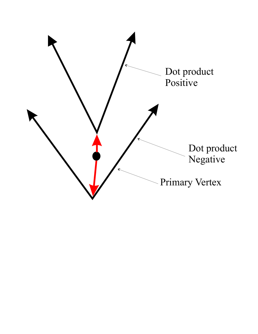
Figure 25: Diagram explaining the effect of $(pt\cdot X_{\nu})>0$ cut

At Level 3, as for $B\rightarrow\pi\pi$ we will at the very least verify Level 2, but we will probably need to do something more sophisticated than this to beat the cross-section down to an acceptable level.

The trigger rates are estimated to be (for the initial configuration of the accelerator) $250nb$ at level1, $560\pm 125nb$ at Level 2, and $200nb$ at Level 3. This would lead to a 200 million event data set size.

References

6.2 A brief outline of the LHCb trigger

C. Shepherd-Themistocleous, Cambridge University

6.2.1 Introduction

B meson decay processes of interest to CP violation physics have small branching ratios, typically of the order of 10^-5. The production of large quantities of B mesons is therefore required for a study of these processes. Such large rates, of the order of 10⁵ $\rm b\bar{b}$ events/s will be available at the LHC collider. The price that has to be paid for these large rates is a very high background rate. The rate of bunch crossings with at least 1 interaction at the LHCb interaction point will be of the order of 12MHz. One of the greatest challenges of the experiment is therefore to be able to trigger on interesting events. The event rate is so high that it is not even possible to record all B events. This therefore means that a highly selective and efficient trigger is required. It also has the important consequence that the designers of the trigger should be aware of all potentially interesting final states while the trigger is being designed. If a particular channel is only found to be of interest at a later date then it is likely that the trigger will be inefficient for this particular channel. While the parts of the trigger that are algorithms running on processors may easily be changed, changing the hardware is a much more difficult task. The strategy that will be followed at the LHCb detector is briefly outlined below.

6.2.2 Trigger strategy at the LHCb experiment

[1]

The beam crossing rate at the LHC is 40MHz and the LHCb trigger is designed to be ready to receive data at every beam crossing. This means that the detectors must be readout at a rate of 40MHz and a trigger decision must also be made a this rate. It is clear that a sophisticated trigger algorithm cannot be run in the 25ns available between beam crossings. The strategy followed therefore is to use a pipeline trigger and to use several different levels of trigger. In a pipeline trigger data are stored for a fixed time while processing is performed to make a trigger decision. The processing takes place in parallel for different events. Therefore, in the first level of the trigger for example, while a decision is made at a frequency of 40MHz, 4$\mu$s are available for each event to be processed.

The Level 0 trigger utilizes the fact that decay products of B decays have on average higher momenta transverse to the beam (p_t) direction than background particles. This trigger looks for high p_t muons, electrons and hadrons as well as photons and possibly neutral pions. These triggers take place in parallel and are then combined into a final Level 0 decision. At this stage a veto trigger on beam crossings that contain more than 1 interaction may also be used. This uses part of the vertex detector to identify multiple primary vertices. This level of the trigger is designed to produced an output of 1MHz.

The next trigger level utilizes the other major characteristic of B mesons, namely their long lifetimes. This leads to a mean decay length of 7mm at LHCb and hence to decay vertices clearly separated from the primary vertex. A silicon vertex detector placed close to the beam pipe is used to look for these secondary vertices.

These first two levels of the trigger are “hardware” triggers in the sense that it will be hard to change these triggers once the detector is built. Any changes would have implications for aspects such as the physical configuration in which the detectors are read out and the speed of operation of specialized chips on electronics boards. The first two levels of the trigger have to operate a high rates and hence essentially use one subdetector in each trigger for speed.

At this point all the data is made available to a processing farm and all subsequent triggers are software algorithms. Data from several subdetectors can now be combined to refine the earlier triggers. An example is the refinement of the vertex trigger. The vertex detector is not in a magnetic field and a source of fake secondary vertices is from multiply scattered low momentum tracks. This background can be removed by using information from tracking chambers. Complete tracking information will also be available to selection algorithms in the trigger. After all generic B selection algorithms the event is rate still too high to allow the recording of all events selected at this point. Once this stage has been reached algorithms to select specific B decays or classes of B decay are performed. Data will finally be written to tape at rate of about 200Hz. An important difference between this trigger and the trigger used in CDF is that analysis of data in the later stages of the trigger is not restricted to regions of interest in the detector that have been defined by earlier stages of trigger. The processing power available here is such that this time saving device is not required.

The discussion about triggers that took place in the CP violation working group proved to be a very useful one. In particular many people where made aware of the difficulty of triggering in the hadron collider environment and of the importance of knowing early in the design phase what final states must be triggered on. Many useful discussions on what ought to be included in the LHCb trigger took place.

References

6.3 Separating $\Upsilon(4\mbox{S})$ decays from continuum events using a neural network

Fabrizio Salvatore and Glen Cowan, Royal Holloway

6.3.1 Introduction

Artificial Neural Networks (NN) have been applied to a variety of problems in high energy physics in order to discriminate between different classes of events. Here the technique is used to separate $b\bar{b}$ events from $\Upsilon(4\mbox{S})$ decays (‘signal’) from the continuum background for $\mbox{e}^{+}\mbox{e}^{-}$ interactions at a centre-of-mass energy $E_{\rm cm}=10.58$ GeV, i.e., at the $\Upsilon(4\mbox{S})$ resonance. The analysis relies on the different topologies for signal and background at a B Factory: while $b\bar{b}$ events are more ‘spherical’, $uds$ and $c\bar{c}$ events are more ‘jet-like’. This is due to the fact that in the $\Upsilon(4\mbox{S})$ rest frame, the momenta of the produced B mesons are small and they decay isotropically. On the other hand, events where light quarks ($u\overline{u}$, $d\overline{d}$ or $s\overline{s}$) are produced are characterized by a preferred direction with hadron jets following roughly the quark and antiquark. A similar jet-like structure is also present in $c\overline{c}$ events, although there it is less pronounced.

For this study, two samples of 600k events of the type $\mbox{e}^{+}\mbox{e}^{-}\rightarrow q\overline{q}$ have been generated using PYTHIA [1] all at a centre-of-mass energy equal to the mass of the $\Upsilon(4\mbox{S})$, where the quark flavour $q$ is a mixture of $u$, $d$ and $s$ in the first set and $c$ in the second. A third data sample of the same size consisted of $\Upsilon(4\mbox{S})$ decays. The analysis has been performed at the level of the generated particles and no attempt has been made at this stage to simulate detector effects.

6.3.2 The shape variables

The variables used to discriminate jet-like from isotropic events are described below. Further information on the variables can be found in [2, 3].

• The ratio $R_{2}=H_{2}/H_{0}$ of the 2nd to the 0th Fox-Wolfram moments. Neglecting particle masses, 4-momentum conservation requires that $H_{0}=1$. For a two-jet event, $H_{1}=0$ and $H_{l}\sim 1$ for $l$ even and $H_{l}\sim 0$ for $l$ odd. The $R_{2}$ distribution is shown in Fig. 26, where the different behaviour for signal and background events can be observed.

• The thrust $T=\sum_{i}|\hat{T}\cdot{\bf p_{i}}|/\sum_{i}|{\bf p_{i}}|$, where $\hat{T}$ is the thrust axis of the event [2]. For an isotropic event one has $T=0.5$ while $T\sim 1$ for a highly directional one, as shown in Figs. 27 (a) and (c).

Figure 26: $R_{2}$ distribution for (a) $\Upsilon(4\mbox{S})$ signal and (b) continuum events.

The variables defined above are quite powerful for identifying events where the two-jet topology is well defined and clearly distinguishable from the isotropic case. The signal to background separation decreases, however, when one or more gluons are emitted, which is more likely to happen when light quarks are produced. In this case there are three or more jets, so that the event shape resembles more that of the signal.

To discriminate further between signal and background, the Durham clustering algorithm [4] is applied to group particles into jets. For every pair of particles $i$ and $j$, the ‘distance’ $y_{ij}$ is computed as

$$y_{ij}=\frac{2~{}\mbox{min}(E_{i}^{2},E_{j}^{2})~{}(1-\cos\theta_{ij})}{E_{\rm vis}^{2}}\,,$$ (118)

where $E_{i}$ and $E_{j}$ are the particles’ energies, $\theta_{ij}$ is their opening angle and $E_{\rm vis}$ is the total (visible) energy in the event. The pair with the smallest $y_{ij}$ is replaced by a pseudo-particle with four-momentum $p^{\mu}=p^{\mu}_{i}+p^{\mu}_{j}$. The procedure is repeated until $N$ jets have been found. In our case $N=3$ or 4 and the smallest $y_{ij}$ values are called $y_{3}$ and $y_{4}$, respectively. Once the clustering has been done, the following discriminating variables can be added to the list:

• $y_{3}$, $y_{4}$;

• $\theta_{\rm BZ}$, the angle between the highest and second highest energy jet;

• $\theta_{\rm KS}$, the angle between the lowest and second lowest energy jet;

• $\theta_{\rm NR}$, the angle between the planes defined by the highest and lowest energy jets and by the other two jets;

• $\theta_{34}$, the angle between the planes defined by the highest and second highest jets and by the other two jets;

• the QCD four-jet matrix element squared, $|M_{QCD}|^{2}$, averaged over all possible assignments of the jets to the final-state partons [5].

As an example, the distribution of $\ln|M_{QCD}|^{2}$ is shown in Fig. 27(b) and (d) for signal and background events.

Figure 27: Distribution of (a) thrust and (b) $\ln|M_{QCD}|^{2}$ (right) for signal events; (c) and (d) show the same for continuum events.

6.3.3 The analysis results

All the variables defined in the previous section have been combined in a Neural Network using the package JETNET 3.51 [6]. The network is a 3 layered feed-forward one, with 9 input nodes, 12 hidden nodes and one output. The network has been trained using 100k $b\bar{b}$, 100k $uds$ and 100k $c\bar{c}$ events. Each input variable has been scaled linearly so that it lies in the range [-1,1]; in this way at the start of the training no single variable dominates the inputs to any neuron. The training algorithm is ‘error back-propagation’.

After the training, the NN has been used with an independent sample of events, 500k for each type, and the output distributions are shown in Fig. 28. The signal and background curves are very well separated, with continuum background events accumulating around 0 and signal events around 1.

Figure 28: Distributions of the NN output for (a) signal and (b) background events. The distributions are superimposed in (c) after being normalized to unity.

To evaluate the rejection power of the NN we can set a cut on the output such that the efficiency for the signal is 90%; this corresponds to requiring an output greater than $0.35$. The fraction of background events surviving the cut is 14% for $uds$ events and 18% for $c\bar{c}$ events.

6.3.4 Conclusions

A feed-forward neural network has been applied to separate $q\overline{q}$ continuum events from $\Upsilon(4\mbox{S})$ decays produced in simulated $\mbox{e}^{+}\mbox{e}^{-}$ interactions at the $\Upsilon(4S)$ resonance. Preliminary results are quite encouraging. For a signal efficiency of 90%, only $\sim 16\%$ of background events survive the NN cut. More work needs to be done to verify that the results are still valid after a full detector simulation; nevertheless, the NN technique seems a promising option for this kind of analysis.

References

7 QCD Factorization

7.1 Factorization in charmless B decays

W.N. Cottingham

Apart from electro-weak terms and other small corrections and taking account of QCD corrections the effective Hamiltonian for b quark decay is a sum of current current terms $j\cdot j$. Factorization approximates the quasi two body sum of matrix elements $\langle h_{1}h_{2}\mid j\cdot j\mid B\rangle$ by a sum over products of single body matrix elements $\langle h_{1}\mid j^{\mu}\mid B\rangle\langle h_{2}\mid j_{\mu}\mid 0\rangle$. So that the transition amplitude [1, 2, 3] becomes

$$\langle h_{1}h_{2}\mid H_{eff}\mid B\rangle=G_{F}/\sqrt{2}\Sigma^{6}_{i}P_{i}[Q_{i}(h_{1},h_{2})+Q_{i}(h_{2},h_{1})]$$

$$Q_{1}(h_{1},h_{2})=\langle h_{1}\mid\bar{u}\gamma^{\mu}(1-\gamma_{5})b\mid B\rangle\langle h_{2}\mid\bar{q}\gamma_{\mu}(1-\gamma_{5})u\mid 0\rangle$$

$$Q_{2}(h_{1},h_{2})=\langle h_{1}\mid\bar{q}\gamma^{\mu}(1-\gamma_{5})b\mid B\rangle\langle h_{2}\mid\bar{u}\gamma_{\mu}(1-\gamma_{5})u\mid 0\rangle$$

$$Q_{3}(h_{1},h_{2})=\langle h_{1}\mid\bar{q}\gamma^{\mu}(1-\gamma_{5})b\mid B\rangle\langle h_{2}\mid\bar{q}^{{}^{\prime}}\gamma_{\mu}(1-\gamma_{5})q^{{}^{\prime}}\mid 0\rangle$$

$$Q_{4}(h_{1},h_{2})=\langle h_{1}\mid\bar{q}^{{}^{\prime}}\gamma^{\mu}(1-\gamma_{5})b\mid B\rangle\langle h_{2}\mid\bar{q}\gamma_{\mu}(1-\gamma_{5})q^{{}^{\prime}}\mid 0\rangle$$

$$Q_{5}(h_{1},h_{2})=\langle h_{1}\mid\bar{q}\gamma^{\mu}(1-\gamma_{5})b\mid B\rangle\langle h_{2}\mid\bar{q}^{{}^{\prime}}\gamma_{\mu}(1-\gamma_{5})q^{{}^{\prime}}\mid 0\rangle$$

$$Q_{6}(h_{1},h_{2})=(-2)\langle h_{1}\mid\bar{q}^{{}^{\prime}}(1-\gamma_{5})b\mid B\rangle\langle h_{2}\mid\bar{q}(1+\gamma_{5})q^{{}^{\prime}}\mid 0\rangle$$

$$q=d,s\hskip 28.45274ptq^{{}^{\prime}}=u,d,s$$

The coefficients $P_{i}$ are constructed from Wilson coefficients [4, 5] and CKM parameters. The Wilson coefficients have been quite reliably estimated from QCD. The single particle matrix elements, for example $\langle\pi^{+}\mid\bar{u}\gamma^{\mu}(1-\gamma_{5})d\mid 0\rangle=f_{\pi}p_{\pi}^{\mu}$, involve soft QCD parameters, in this case $f_{\pi}$ and many are quite precisely known for example from measured leptonic decay rates. The matrix elements $\langle h_{1}\mid j^{\mu}\mid B\rangle$ are in principle measurable from B semi leptonic decays, they involve only a few parameters. For the moment they are only available as theoretical estimates.

The physical justification for the factorisation approximation is the idea of colour transparency. It is argued that the b quark by virtue of its large mass imparts a large velocity to the light quark decay products, the pair which form the light particle $h_{2}$ move away but stay together as a colour singlet so escape from the gluonic environment of the B meson without interaction as does a lepton pair in the semi leptonic decay $B\rightarrow h_{1}+l+\nu$ which is described by a matrix element $\langle h_{1}\mid j^{\mu}\mid B\rangle$. This rationale has recently been given theoretical justification [3], it has been claimed that for decays into a pair of light mesons and in the heavy quark limit that the corrections to the factorisation approximation can be calculated from first principles of perturbative QCD. The corrections involve, as you might expect, hard gluon interactions with the spectator quark but the only long distance physics, other than the current matrix elements, involves the meson light cone distribution amplitudes. The beauty of the results presented in [3] for $\pi\pi$ decay is that the coefficients $P_{i}$ acquire additional perturbative corrections. The difference between the decay rate formulae of the factorisation approximation and the formulae with the QCD corrections lies only in the coefficients $P_{i}$, the factorisation matrix elements are common to both. Generalisations to other decay channels can be found in [5, 6, 7].

The corrections to the coefficients $P_{i}$ so far presented are to first order in $\alpha_{s}$. An encouraging feature is that they are not large, which leads one to hope that the precision with which the standard model can be tested will be determined by the proximity of the b quark mass to the heavy quark limit and the precision of our knowledge of the soft QCD parameters, B meson semileptonic transition form factors, meson light cone distribution amplitudes etc. Because of the involvement of soft QCD parameters, some of which are only poorly known, and to be confident of the conclusions about the standard model, it will be important to have a consistent picture of as many channels of charmless B decay as possible.

Limiting the discussion to the light hadrons $h_{1}$ and $h_{2}$ being the lowest mass pseudo scaler and vector mesons there are only a few poorly known soft QCD parameters. Because the B has zero spin a spin one meson with a spin zero partner is confined to the helicity zero state. Also in the heavy quark limit and to lowest order in $\left(m_{h}/m_{B}\right)^{2}$ only helicity zero states should be involved in transitions to two spin one mesons . The poorly known B transition form factors should then involve only five parameters that describe the transitions $B\rightarrow\pi,B\rightarrow\rho,B\rightarrow\omega,B\rightarrow K,B\rightarrow K^{*}$ Setting aside transitions involving the $\eta$ and $\eta^{{}^{\prime}}$ there are about forty channels of $B^{0}$ and $B^{+}$ decay with branching ratios anticipated to be greater than $10^{-6}$ [2]. It can be expected that the basic validity of the improved factorisation approximation will be tested within the next year or two, and the proximity of the b quark mass to the heavy quark limit will determine the sharpness of focus that this method provides on the standard model description of the weak interaction.

References

7.2 Phenomenological impact of the QCD improved factorization approach
Content identical to [1]

M. Beneke, RWTH Aachen

7.2.1 Introduction

The observation of $B$ decays into $\pi K$ and $\pi\pi$ final states has resulted in a large amount of theoretical and phenomenological work that attempts to interpret these observations in terms of the factorization approximation (FA), or in terms of general parameterizations of the decay amplitudes. A detailed understanding of these amplitudes would help us to pin down the value of the CKM angle $\gamma$ using only data on CP-averaged branching fractions. Theoretical work on the heavy-quark limit has justified the FA as a useful starting point [2, 3], but predicts important and computable corrections. Here we discuss the most important consequences of this approach for the $\pi K$ and $\pi\pi$ final states.

To leading order in an expansion in powers of $\Lambda_{\rm QCD}/m_{b}$, the $B\to\pi K$ matrix elements obey the factorization formula

$$\langle\pi K|Q_{i}|B\rangle = f_{+}^{B\to\pi}(0)\,f_{K}\,T_{K,i}^{\rm I}*\Phi_{K}$$

$$\mbox{}+f_{+}^{B\to K}(0)\,f_{\pi}\,T_{\pi,i}^{\rm I}*\Phi_{\pi}$$

$$\mbox{}+f_{B}f_{K}f_{\pi}\,T_{i}^{\rm II}*\Phi_{B}*\Phi_{K}*\Phi_{\pi}\,,$$

where $Q_{i}$ is an operator in the weak effective Hamiltonian, $f_{+}^{B\to M}(0)$ are semi-leptonic form factors of a vector current evaluated at $q^{2}=0$, $\Phi_{M}$ are leading-twist light-cone distribution amplitudes, and the $*$-products imply an integration over the light-cone momentum fractions of the constituent quarks inside the mesons. When the hard-scattering functions $T$ are evaluated to order $\alpha_{s}^{0}$, Eq. (7.2.1) reduces to the conventional FA. The subsequent results are based on kernels including all corrections of order $\alpha_{s}$. A detailed justification of (7.2.1) is given in Ref. [3]. Compared to our previous discussion of $\pi\pi$ final states[2] the present analysis incorporates three new ingredients:

i) the matrix elements of electroweak (EW) penguin operators (for $\pi K$ modes);

ii) hard-scattering kernels for general, asymmetric light-cone distributions;

iii) the complete set of “chirally enhanced” $1/m_{b}$ corrections [2].

The second and third items have not been considered in other [4] generalizations of Ref. [2] to the $\pi K$ final states. The third one, in particular, is essential for estimating some of the theoretical uncertainties of the approach.

We now briefly present the input to our calculations. Following Ref. [2], we obtained the coefficients $a_{i}(\pi K)$ of the effective factorized transition operator defined analogously to the case of $\pi\pi$ final states, but augmented by coefficients $a_{7-10}(\pi K)$ related to EW penguin operators and electro-magnetic penguin contractions of current–current and QCD penguin operators. A sensible implementation of QCD corrections to EW penguin matrix elements implies that one departs from the usual renormalization-group counting, in which the initial condition for EW penguin coefficients is treated as a next-to-leading order (NLO) effect. Our NLO initial condition hence includes the $\alpha_{s}$ corrections computed in Ref. [5].

Chirally enhanced corrections arise from twist-3 two-particle light-cone distribution amplitudes, whose normalization involves the quark condensate. The relevant parameter, $2\mu_{\pi}/m_{b}=-4\langle\bar{q}q\rangle/(f_{\pi}^{2}m_{b})$, is formally of order $\Lambda_{\rm QCD}/m_{b}$, but large numerically. The coefficients $a_{6}$ and $a_{8}$ are multiplied by this parameter. There are also additional chirally enhanced corrections to the spectator-interaction term in (7.2.1), which turn out to be the more important effect. In both cases, these corrections involve logarithmically divergent integrals, which violate factorization. For instance, for matrix elements of $V-A$ operators the hard spectator interaction is now proportional to ($\bar{u}\equiv 1-u$)

$$\int_{0}^{1}\!\frac{du}{\bar{u}}\frac{dv}{\bar{v}}\,\Phi_{K}(u)\left(\Phi_{\pi}(v)+\frac{2\mu_{\pi}}{m_{b}}\frac{\bar{u}}{u}\right)$$

when the spectator quark goes to the pion. (Here we used that the twist-3 distribution amplitudes can be taken to be the asymptotic ones when one neglects twist-3 corrections without the chiral enhancement.) The divergence of the $v$-integral in the second term as $\bar{v}\to 0$ implies that it is dominated by soft gluon exchange between the spectator quark and the quarks that form the kaon. We therefore treat the divergent integral $X=\int_{0}^{1}(dv/\bar{v})$ as an unknown parameter (different for the penguin and hard scattering contributions), which may in principle be complex owing to soft rescattering in higher orders. In our numerical analysis we set $X=\ln(m_{B}/0.35\,\mbox{GeV})+r$, where $r$ is chosen randomly inside a circle in the complex plane of radius 3 (“realistic”) or 6 (“conservative”). Our results also depend on the $B$-meson parameter[2] $\lambda_{B}$, which we vary between 0.2 and 0.5 GeV. Finally, there is in some cases a non-negligible dependence of the coefficients $a_{i}(\pi K)$ on the renormalization scale, which we vary between $m_{b}/2$ and $2m_{b}$.

7.2.2 Results

We take $|V_{ub}/V_{cb}|=0.085$ and $m_{s}(2\,\mbox{GeV})=110\,$MeV as fixed input, noting that ultimately the ratio $|V_{ub}/V_{cb}|$, along with the CP-violating phase $\gamma=\mbox{arg}(V_{ub}^{*})$, might be extracted from a simultaneous fit to the $B\to\pi K$ and $B\to\pi\pi$ decay rates.

$SU(3)$ breaking

Bounds[6, 7] on the CKM angle $\gamma$ derived from ratios of $\pi K$ branching fractions, as well as the determination of $\gamma$ using the method of Ref. [8], rely on an estimate of $SU(3)$ flavour-symmetry violations. We find that “non-factorizable” $SU(3)$-breaking effects (i.e., effects not accounted for by the different decay constants and form factors of pions and kaons in the conventional FA) do not exceed a few percent at leading power.

Amplitude parameters

The approach discussed here allows us to obtain the decay amplitudes for the $\pi\pi$ and $\pi K$ final states in terms of the form factors and the light-cone distribution amplitudes. The $\pi^{0}\pi^{0}$ final state is very poorly predicted and will not be discussed here. We write

$${\cal A}(B^{0}\to\pi^{+}\pi^{-})=T\,[e^{i\gamma}+(P/T)_{\pi\pi}]$$

and parametrize the $\pi K$ amplitudes by[7]

$${\cal A}(B^{+}\to\pi^{+}K^{0}) = P\left(1-\varepsilon_{a}\,e^{i\eta}e^{i\gamma}\right),$$

$$-\sqrt{2}\,{\cal A}(B^{+}\to\pi^{0}K^{+}) = P\Big{[}1-\varepsilon_{a}\,e^{i\eta}e^{i\gamma}-\varepsilon_{3/2}\,e^{i\phi}(e^{i\gamma}-q\,e^{i\omega})\Big{]},$$ (120)

$$-{\cal A}(B^{0}\to\pi^{-}K^{+}) = P\Big{[}1-\varepsilon_{a}\,e^{i\eta}e^{i\gamma}-\varepsilon_{T}\,e^{i\phi_{T}}(e^{i\gamma}-q_{C}\,e^{i\omega_{C}})\Big{]},$$

and $\sqrt{2}\,{\cal A}(B^{0}\to\pi^{0}K^{0})={\cal A}(B^{+}\to\pi^{+}K^{0})+\sqrt{2}\,{\cal A}(B^{+}\to\pi^{0}K^{+})-{\cal A}(B^{0}\to\pi^{-}K^{+})$. Table 15 summarizes the numerical values for the amplitude parameters for the conservative variation of $X$, and variation of the other parameters as explained above. The LO results correspond to the conventional FA at the fixed scale $\mu=m_{b}$. They are strongly scale dependent. In comparison, the scale-dependence of the NLO result is small, with the exception of $q_{C}\,e^{i\omega_{C}}$. One must keep in mind that the ranges may overestimate the true uncertainty, since the parameter $X$ may ultimately be constrained from a subset of branching fractions. This is true in particular for the quantity $\varepsilon_{3/2}$ in Table 15, which can be extracted from data.[7]

	Range, NLO	LO
$-\varepsilon_{a}\,e^{i\eta}$	$(0.017\mbox{--}0.020)\,e^{i\,[13,21]^{\circ}}$	$0.02$
$\varepsilon_{3/2}\,e^{i\phi}$	$(0.20\mbox{--}0.38)\,e^{i\,[-30,7]^{\circ}}$	$0.36$
$q\,e^{i\omega}$	$(0.53\mbox{--}0.63)\,e^{i\,[-7,3]^{\circ}}$	$0.64$
$\varepsilon_{T}\,e^{i\phi_{T}}$	$(0.20\mbox{--}0.29)\,e^{i\,[-19,3]^{\circ}}$	$0.33$
$q_{C}\,e^{i\omega_{C}}$	$(0.00\mbox{--}0.22)\,e^{i\,[-180,180]^{\circ}}$	$0.06$
$(P/T)_{\pi\pi}$	$(0.19\mbox{--}0.29)\,e^{i\,[-1,23]^{\circ}}$	$0.16$

Table 15: Parameters for the $B\to\pi K$ amplitudes as defined in (7.2.2), for conservative variation of all input parameters (see text).

Ratios of CP-averaged rates

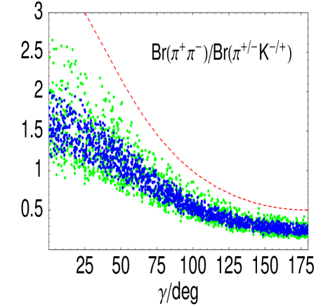
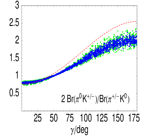
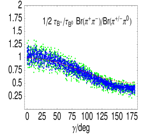
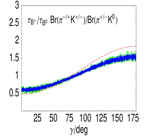
Figure 29: Ratios of CP-averaged $B\to\pi K$ and $\pi\pi$ decay rates. The scattered points cover a realistic (dark) and conservative (light) variation of input parameters. The dashed curve is the LO result, corresponding to conventional factorization.

Since the form factor $f_{+}(0)$ is not well known, we consider here only ratios of CP-averaged branching ratios, discarding the $\pi^{0}\pi^{0}$ final state. We display these as functions of the CKM angle $\gamma$ in Fig. 29.

Table 15 shows that the corrections with respect to the conventional FA are significant (and important to reduce the renormalization-scale dependence). Despite this fact, the qualitative pattern that emerges for the set of $\pi K$ and $\pi\pi$ decay modes is similar to that in conventional factorization. In particular, the penguin–tree interference is constructive (destructive) in $B\to\pi^{+}\pi^{-}$ ($B\to\pi^{-}K^{+}$) decays if $\gamma<90^{\circ}$. Taking the currently favoured range $\gamma=(60\pm 20)^{\circ}$, we find the following robust predictions:

$$\frac{\mbox{Br}(\pi^{+}\pi^{-})}{\mbox{Br}(\pi^{\mp}K^{\pm})} = 0.5\mbox{--}1.9\quad[0.25\pm 0.10]$$

$$\frac{\mbox{Br}(\pi^{\mp}K^{\pm})}{2\mbox{Br}(\pi^{0}K^{0})} = 0.9\mbox{--}1.4\quad[0.59\pm 0.27]$$

$$\frac{2\mbox{Br}(\pi^{0}K^{\pm})}{\mbox{Br}(\pi^{\pm}K^{0})} = 0.9\mbox{--}1.3\quad[1.27\pm 0.47]$$

$$\frac{\tau_{B^{+}}}{\tau_{B^{0}}}\,\frac{\mbox{Br}(\pi^{\mp}K^{\pm})}{\mbox{Br}(\pi^{\pm}K^{0})} = 0.6\mbox{--}1.0\quad[1.00\pm 0.30]$$

The first ratio is in striking disagreement with current CLEO data[10] (square brackets). The near equality of the second and third ratios is a result of isospin symmetry.[7] We find $\mbox{Br}(B\to\pi^{0}K^{0})=(4.5\pm 2.5)\times 10^{-6}\,(V_{cb}/0.039)^{2}(f^{B\to\pi}_{+}(0)/0.3)^{2}$ almost independently of $\gamma$. This is three time smaller than the central value reported by CLEO.

CP asymmetry in $B\to\pi^{+}\pi^{-}$ decay

The stability of the prediction for the $\pi^{+}\pi^{-}$ amplitude suggests that the CKM angle $\alpha$ can be extracted from the time-dependent mixing-induced CP asymmetry in this decay mode, without using isospin analysis. Fig. 30 displays the coefficient $S$ of $-\sin(\Delta M_{B_{d}}t)$ as a function of $\sin(2\alpha)$ for $\sin(2\beta)=0.75$, which may be compared with the result in Ref. [9]. For some values of $S$ there is a two-fold ambiguity (assuming all angles are between $0^{\circ}$ and $180^{\circ}$). A consistency check of the approach could be obtained, in principle, from the coefficient of the $\cos(\Delta m_{B_{d}}t)$ term.

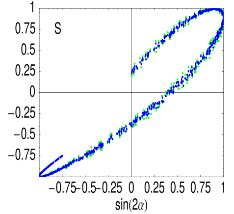
Figure 30: Mixing-induced CP asymmetry in $B\to\pi^{+}\pi^{-}$ decays. The lower band refers to values $45^{\circ}<\alpha<135^{\circ}$, the upper one to $\alpha<45^{\circ}$ (right) or $\alpha>135^{\circ}$ (left). We assume $\alpha,\beta,\gamma\in[0,\pi]$.

7.2.3 Conclusions

We have examined some of the consequences of the QCD factorization approach to $B$ decays into $\pi K$ and $\pi\pi$ final states, leaving a detailed discussion to a subsequent publication. Here we have focused on robust predictions for ratios of CP-averaged decay rates. Our result for the ratio of the $B\to\pi^{+}\pi^{-}$ and $B\to\pi^{\mp}K^{\pm}$ decay rates is in disagreement with the current experimental value, unless the weak phase $\gamma$ were significantly larger than $90^{\circ}$.

References

8 Statistical Errors

8.1 Feldman and Cousins for Pedestrians

R. Barlow, University of Manchester

“What confidence is this wherein thou trustest?”

Isaiah Chap. 36 v. 4

8.1.1 What is a confidence level?

Confidence levels are the subject of much confusion and argument. To bring out what they are, and what they are not, consider two statements which might validly be made with 90% confidence. (For illustration this note uses 90% confidence levels throughout, but of course any value can be chosen.)

A grocer: “Our potatoes weigh between $100$ and $400g$.”

A physicist:“The Higgs Boson has a mass between $100$ and $400GeV/c^{2}$.

The superficial similarity conceals a difference. The grocer has weighed many potatoes and found that 90% of them have weights in the limits given. The statement has a 90% probability of being true, with probability defined in the conventional (frequentist) way as

$$P=\lim_{N\to\infty}{N_{InRange}^{objects}\over N_{Total}^{objects}}$$

The physicist has not weighed any Higgs Bosons. If they had, they would discover either that all the bosons are within the range, or that all the bosons are outside it. Equation (1) will give a probability which is either 0 or 1. What they mean by a 90% confidence level statement is not

“A Higgs boson mass has a 90% probability of lying between $100$ and $400GeV/c^{2}$”

but

“The statement ‘The Higgs Boson Mass lies between $100$ and $400GeV/c^{2}$’ has a 90% probability of being true.”

If this physicist goes through life making statements of this type, they will be correct in 9 cases out of 10. The ‘probability’ of 90% is still given as the limit of a frequency, but a rather different one.

$$P=\lim_{N\to\infty}{N_{True}^{statements}\over N_{Total}^{statements}}$$

As a technical detail, a confidence level of 90% actually means that the probability is at least 90% (this covers cases in which it is not calculable exactly.) So they are right at least 9 times out of 10.

8.1.2 Frequentist confidence levels

The basic tool for constructing confidence intervals is the Confidence Diagram[2]. Suppose that a parameter of interest $a$ and an observed quantity $x$ are related by a pdf $P(x;a)$. (For example: $x$ could be a number of events, and $a$ a branching ratio.)

Choose a value of the probability (e.g. 68%, 90%, 95%) and a strategy (e.g. one sided upper, one sided lower, two-sided symmetrical). For any value of $a$, we can make statements about the probability of $x$ lying in certain regions, and determine a range $[x_{-},x_{+}]$ within which we say (at the desired level of confidence) that $x$ will lie.

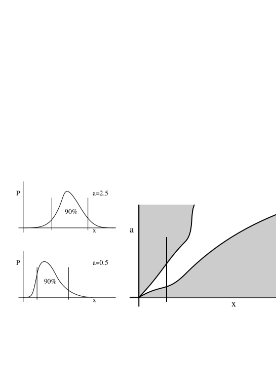
Figure 31: A two-sided confidence band.

We then plot $x_{-}$ and $x_{+}$ on the diagram as a function of $a$. Suppose we chose to quote 90% central confidence limits. Any horizontal line across the plot represents a particular value of $a$ and thus a pdf with its limits, as shown in two particular cases. There is a 5% chance of a measurement lying below the lower limit, and a 5% chance of it lying above the upper limit. The unshaded region between the limits is the confidence band (or belt).

The next step is a neat bit of logic. For any value of $a$, the probability that $x$ lies in the belt is, by construction, 90%. So if you make an observation $x$ the probability of the pair $(x,a)$ lying within the belt is $90\%$. A vertical line at the observed $x$ gives the limits for $a$ where it intersects the edges of the confidence belt.

A similar technique gives one sided (upper) limits: for each value of $a$ the value of $x$ is found for which the probability of a result this small or smaller is only 10% (or whatever), and for a measured $x$ you read off the upper limit $a_{+}$ for which the probability of such a low result is only 10% – for a higher value of $a$ the probability is even smaller.

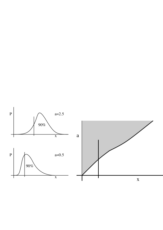
Figure 32: A one-sided confidence band.

8.1.3 Poisson statistics

This theory of confidence limits applies to any distribution function, but in B physics its main use is in dealing with rare decays, where observed numbers of events are governed by Poisson statistics. This means that the variable $x$ is discrete (integer) – denote it by $N$. Confidence diagrams have a continuous ordinate but a discrete abscissa and the smooth curves become staircases. Integrations are replaced by summations. For an observed number $N$ the limits are given by

$$\sum_{0}^{N}P(r;a_{+})=0.05\qquad\sum_{0}^{N-1}P(r;a_{-})=0.95$$

This means that in general it won’t be possible to find a range which satisfies $\sum P(r;a)=0.05$. One has to use the conservative requirement $\sum P(r;a)\leq 0.05$.

$a$ is a branching ratio, lifetime, or similar quantity describing a source of events. It trivially translates into a number of events $S$. The actual expected number is then often given by $S+B$, where $B$ is some background which we will take as being reliably and accurately estimated. The probability of observing $r$ events is the Poisson expression

$$e^{-(S+B)}(S+B)^{r}/r!$$

8.1.4 Problem: non-physical regions

Often this works perfectly well, but there are problems if the parameter estimates lie near some physical boundary. (For example Branching Ratios cannot be negative. Another relevant example is the interpretation of the limit on the Higgs mass from precision electroweak measurements when much of the range is already ruled out by direct searches.)

For example, if $B$ is 5.1, and you observe 1 event, what can you conclude about $S$? Following the above procedure, you calculate $0.05=\sum_{0}^{1}P(r;4.74)=\sum_{1}^{\infty}P(r;0.05)$ so $S+B$ lies between $0.05$ and $4.74$, so you can say with 90% confidence that $S$ lies between $-5.05$ and $-0.36$. One would have to be an extreme purist to publish such a statement. It is technically correct: you expect one in ten of your 90% CL statements to be wrong. In this case you just have independent confirmation that this is one of them; you happen to have had a large downward fluctuation in the background. There is no way of including the knowledge that $S$ must be non-negative.

8.1.5 Bayesian confidence levels

Bayesian statistics[3] handles these limits without problems using Bayes’ theorem.

$$P(a;x)={P(x;a)\over P(x)}P(a)$$

here $P(x;a)$ is the usual pdf. $P(x)$ is a prior distribution for $x$, usually ignored as being taken care of by normalisation. $P(a)$ is the prior probability for $a$. A full discussion of Bayesian versus Frequentist methodologies can be found in [4].

The probabilities $P(a)$ and $P(a;x)$ do not have a frequentist definition (except as a delta function) but can be defined as subjective probabilities. The form of $P(a)$ is often taken as uniform, under the ‘principle of ignorance’; this title is disingenuous as the assumption of a prior uniform in, say a lifetime $\tau$ will lead to different limits than those obtained from a prior uniform in, say, the width $\hbar/\tau$. According to Jeffreys’ prescription one should take a uniform distribution for a location parameter, whereas for a scale parameter $\lambda$ the distribution should be proportional to ${1\over\lambda}$ (i.e. uniform in $\ln\lambda$) [6]. Jeffreys’ criteria [7] suggests that for a Poisson source $S$ the appropriate prior should be taken as proportional to ${1\over\sqrt{S}}$.

With a step-function prior (zero for negative values and uniformly constant for positive ones), the requirement for a one-sided confidence limit $S$ on the signal at the level $\alpha$ from $N$ observed events with expected background $B$

$$\alpha=\int_{0}^{S}P(S^{\prime}|N)\,dS^{\prime}$$

produces (after repeated integration by parts) the requirement

$$1-\alpha={\sum_{0}^{N}P(r;B+S)\over\sum_{0}^{N}P(r;B)}$$

which is found in early versions of the PDG [5]. For large $N$, the denominator approaches the standard value of 1. For small $N$ it expresses the fact that we have manifestly got a downward fluctuation of the background, and one should temper the requirement on the signal accordingly.

8.1.6 What Feldman and Cousins do

Feldman and Cousins [1] get us out of this dilemma by pointing out another one.

In real life, physicists (being human) do not decide beforehand whether they will quote a one-sided or a two-sided limit. If the observations are high, a two-tailed limit will be appropriate; if they are low then a single upper limit is the best information that can be given.

For example: given a background of 1.1, if you observed 10 events you would very possibly quote as a result the range of 4.3 to 15.1 (at 90% confidence). If you observed 2 events you would probably say (with 90% confidence) that any signal was less than 4.2. There is some intermediate value at which you would ‘flip-flop’ between the two states.

This may be sensible, but it destroys the confidence belt logic. For small $x$ values we have the one sided belt of Figure 32; for large values the two-sided belt of Figure 31. The resulting hybrid (Figure 33) violates the basis on which the curves were constructed, as for the intermediate values of $a$ the probability content of the belt is not the specified 90%.

Figure 33: The effect of ’flip-flop’.

Feldman and Cousins thus argue that the strategy for deciding whether to quote a one-sided or two-sided result must be decided beforehand, and decided in such a way that for all values of $a$ the probability content of the belt is 90%. They propose a ‘unified approach’ in which a single algorithm decides whether to quote one-sided or two-sided limits, and gives the value(s) in question.

There are an infinite number of solutions for limits $x_{1}$ and $x_{2}$ satisfying

$$\int_{x_{1}}^{x_{2}}P(x;a)\,dx=0.90$$

(For discrete processes $\sum_{r_{1}}^{r_{2}}P(r;a)\geq 0.90$)

One initially plausible algorithm is to include the region where the pdf itself is greatest, adjusting $C$ to satisfy

$$\int_{P(x;a)>C}P(x;a)\,dx=0.90$$

This in fact gives the most compact region.

But consider an outcome with 1 events seen, with an expected signal and background of 0 and 15.1 respectively. This is very unlikely ($4\,10^{-6}$ probability) and this algorithm is bound to exclude the possibility. But given one observed event and a background of 15.1, any probabilities are going to be pretty small, and we would want to include 0 signal in the band, on the grounds that for any other values the probability is even lower! It would be fairer to include points by comparing their probability to, say, the best that can be achieved.

$$\int_{P(x;a)/P(x;a_{best})>C}P(x;a)=0.90$$

For Poisson processes with a known background $B$ and unknown signal $S$, $S_{best}$ is $x-B$, if the observed number is bigger than the expected background, and $0$ if it is smaller.

A Feldman-Cousins confidence interval for rare decays is thus constructed as previously, with a 90% (or whatever) confidence band being constructed for each value of the source strength $S$. For each $S$ the Poisson probability is calculated for each number of observed events $r=0,1,2\dots$, and its ratio taken to the ‘best’ probability (with $S=r-B$ or $S=0$ as appropriate). $r$ values are included in the confidence belt in order of their ranking in this ratio until the total probability condition is fulfilled. The result is a diagram where low values of $N$ will just give one limit whereas higher ones give a range, and the probability content of the belt is valid.

There is a loss of universality as such confidence diagrams, unlike those of the previous scheme, are non-trivially different for different background values.

8.1.7 Some examples

90% confidence intervals are shown for various values for an observed signal and expected background. Both 1-tailed and 2-tailed limits are given for conventional frequentist confidence intervals, and for Bayesian intervals, and Bayesian intervals are shown both for a step-function prior (uniform for positive values) and a prior according to Jeffreys’ prescription, proportional to $1/\sqrt{s}$. (Taking a prior proportional to $1/s$ gives divergent integrals.)

$N$	$B$	Conventional		Uniform Bayesian		Jeffreys’ Bayesian		Feldman-
		1 Tailed	2 tailed	1 Tailed	2 Tailed	1 Tailed	2 Tailed	Cousins
$10$	$0.0$	$<15.4$	$5.43\dots 17.0$	$<15.4$	$6.17\dots 17.0$	$<14.8$	$5.80\dots 16.3$	$5.50\dots 16.5$
	$1.0$	$<14.4$	$4.43\dots 16.0$	$<14.4$	$5.17\dots 16.0$	$<13.7$	$4.73\dots 15.3$	$4.50\dots 15.5$
	$5.0$	$<10.4$	$0.425\dots 12.0$	$<10.4$	$1.43\dots 12.0$	$<9.24$	$0.345\dots 10.8$	$1.19\dots 11.5$
	$10.$	$<5.41$	$-4.57\dots 6.96$	$<6.63$	$0.233\dots 8.08$	$<4.73$	$0.0106\dots 6.15$	$<6.50$
	$15.$	$<0.407$	$-9.57\dots 1.96$	$<4.83$	$0.124\dots 6.10$	$<3.07$	$0.00498\dots 4.21$	$<2.65$
$5$	$0.0$	$<9.27$	$1.97\dots 10.5$	$<9.27$	$2.61\dots 10.5$	$<8.64$	$2.29\dots 9.84$	$1.84\dots 9.99$
	$0.50$	$<8.77$	$1.47\dots 10.0$	$<8.77$	$2.11\dots 10.0$	$<8.07$	$1.71\dots 9.27$	$1.53\dots 9.49$
	$2.5$	$<6.77$	$-0.530\dots 8.01$	$<6.85$	$0.558\dots 8.09$	$<5.66$	$0.0580\dots 6.87$	$<7.49$
	$4.0$	$<5.27$	$-2.03\dots 6.51$	$<5.72$	$0.244\dots 6.92$	$<4.25$	$0.0127\dots 5.42$	$<5.99$
	$10.$	$<-0.725$	$-8.03\dots 0.513$	$<3.71$	$0.0907\dots 4.73$	$<2.30$	$0.00356\dots 3.19$	$<1.83$
$1$	$0.0$	$<3.89$	$0.0513\dots 4.74$	$<3.89$	$0.355\dots 4.74$	$<3.13$	$0.176\dots 3.91$	$0.104\dots 4.36$
	$0.50$	$<3.39$	$-0.449\dots 4.24$	$<3.51$	$0.141\dots 4.36$	$<2.48$	$0.00782\dots 3.25$	$<3.86$
	$1.0$	$<2.89$	$-0.949\dots 3.74$	$<3.27$	$0.100\dots 4.11$	$<2.18$	$0.00442\dots 2.93$	$<3.36$
	$5.0$	$<-1.11$	$-4.95\dots-0.256$	$<2.67$	$0.0615\dots 3.45$	$<1.60$	$0.00237\dots 2.25$	$<1.20$
	$10.$	$<-6.11$	$-9.95\dots-5.26$	$<2.51$	$0.0564\dots 3.25$	$<1.48$	$0.00217\dots 2.10$	$<0.672$
$0$	$0.0$	$<2.30$	$None$	$<2.30$	$0.0513\dots 3.00$	$<1.35$	$0.00196\dots 1.92$	$<2.43$
	$0.10$	$<2.20$	$None$	$<2.30$	$0.0513\dots 3.00$	$<1.35$	$0.00196\dots 1.92$	$<2.33$
	$1.0$	$<1.30$	$None$	$<2.30$	$0.0513\dots 3.00$	$<1.35$	$0.00196\dots 1.92$	$<1.61$
	$5.0$	$<-2.70$	$None$	$<2.30$	$0.0513\dots 3.00$	$<1.35$	$0.00196\dots 1.92$	$<0.770$
$9$	$3.7$	$<10.5$	$0.995\dots 12.0$	$<10.5$	$1.82\dots 12.0$	$<9.49$	$0.775\dots 11.0$	$1.49\dots 11.6$
$9$	$3.7$	$<12.0$	$0.415\dots 13.4$	$<12.0$	$1.24\dots 13.4$	$<11.0$	$0.306\dots 12.3$	$0.994\dots 13.1$
$9$	$3.7$	$<7.49$	$2.37\dots 9.39$	$<7.51$	$3.25\dots 9.40$	$<6.51$	$2.22\dots 8.39$	$2.64\dots 9.09$

Table 16: Some examples of 90% confidence limits for various values

It can be seen that where the signal is safely larger than the background, all methods are in broad agreement. Differences are a salutary reminder of the inevitable arbitrariness of any analysis.

As signal sinks below background, the conventional limits become manifestly erroneous. The Bayesian limits appear more sensible, though the differences between the two versions become larger. The Feldman-Cousins value(s) flip nicely.

8.1.8 Some objections

The new technique has been warmly welcomed by some, but has been criticised by others.

In the 1-sided regime the limit decreases with the value of the expected background, as can be seen from the table. This is apparently counterintuitive: for 2 experiments with the same number of events seen the one with worse (i.e. higher) background has the better (i.e. lower) limit! The counterargument is that the inferior experiment has to be very lucky to see so few events. On average, an experiment with a higher background will see more events and thus give a higher limit: some experiments will always be more fortunate than others, and by increasing $B$ for fixed $N$ you are increasing the experimental luck.

The method does not cope cleanly with the case of zero observed events. This is always going to be a special case because, uniquely, if you observe 0 events you know the number of signal events (zero), and all the background information is irrelevant. Modifications of the method have been suggested to get over this problem [8].

The method can flip to the two sided form in cases the physicist knows are inappropriate. When counting decays forbidden by the standard model, or even by basic conservation laws, the algorithm will give a two sided limit in cases (like 10 events on a background of 5) which are obviously just upward fluctuations of background. Here the experimenter is probably overstretching the applicability of the method. For more plausible decay channels the same experimenter would probably be happy to report a limit from the same data (10 on 5). The method, by its nature, knows only about the numbers and not about the physics.

Broadly speaking (and with some exceptions), frequentists accept the Feldman Cousins method as an improvement on the original form, though it does still have some drawbacks. Bayesians dislike it, perhaps because it expands the scope of frequentist analysis in an area where previously Bayesian technique had a monopoly.

8.1.9 Some questions

Can this method be adapted to the setting of limits on the ratio of two numbers, as was done by James and Roos [9] for the conventional frequentist confidence level?

When one is tuning cuts in an analysis, one aims to optimise signal/background or signal/(signal+background), depending on whether you are questioning the presence of a signal, or measuring the size of a signal you know to be there. Could a similar unified approach be found here?

The unified approach prevents the experimenter flip-flopping between limit strategies, but still leaves the choice of confidence level free. An experimenter who normally used 90% limits may choose to present 68% limits if they obtain a low result where they believe there should be a signal, or 95% or 99% limits if they obtain a high result where they believe no signal should be. Is there some natural way of incorporating this (undesirable?) freedom in an algorithm?

References

8.2 Statistical issues in heavy flavour physics

Glen Cowan, Royal Holloway, University of London

8.2.1 Introduction

In this paper two statistical issues are addressed that come up in many physics analyses but which are particularly relevant for heavy flavour physics. The first, presented in Section 8.2.2, is the problem of combining measurements of the branching ratios of rare decays where some of the measurements are based on only a few or perhaps no candidate events. The solution recommended is a straightforward application of the method of maximum likelihood. The next question, discussed in Section 8.2.3, is much more open-ended, namely, how to quantify theoretical uncertainties. Both issues are of course not unique to heavy flavour physics, and the approaches recommended can be applied in many other contexts.

8.2.2 Combining branching ratios for rare decays

Consider first a single experiment in which one searches for rare decay and finds $n$ candidate events out of $N$ total decays. Suppose the efficiency for the signal is $\varepsilon$ and there are $b$ expected background events. In general, $n$ should be treated as a binomially distributed variable where $N$ represents the total number of trials and the binomial probability ${\cal B}$ is the branching ratio. If ${\cal B}$ is very small and $N$ very large, however, we can treat $n$ as following a Poisson distribution with expectation value $\nu$, i.e.,

$$P(n;\nu)=\frac{\nu^{n}}{n!}e^{-\nu}\;.$$ (121)

Here the number of events observed $n$ is the sum of $n_{s}$ signal and $n_{b}$ background events and the expectation value of $n$, here called $\nu$, is also the sum of the signal and background expectation values $s$ and $b$:

$$n = n_{s}+n_{b}\;,$$ (122)

$$\nu = s+b\;.$$ (123)

The branching ratio ${\cal B}$, which is the parameter we want to estimate, is related to the expected number of signal events $s$, the efficiency $\varepsilon$ and the total number of events $N$ by

$${\cal B}=\frac{s}{\varepsilon N}\;.$$ (124)

For a single experiment, the likelihood function $L({\cal B})$ is simply the Poisson probability (121) evaluated with the observed number of events $n$ and expressed as a function of the branching ratio ${\cal B}$. Maximizing $L$ gives the maximum likelihood (ML) estimator $\hat{{\cal B}}$,

$$\hat{{\cal B}}=\frac{n-b}{\varepsilon N}\;,$$ (125)

where here estimators will be denoted by hats. The statistical uncertainty in $\hat{{\cal B}}$ can be quantified by giving an estimate of its standard deviation,

$$\hat{\sigma}_{\hat{{\cal B}}}=\frac{\sqrt{n}}{\varepsilon N}\;,$$ (126)

or by reporting a confidence interval (see e.g. [1]).

Now consider the case where we have $m$ independent measurements of the branching ratio ${\cal B}$. The $m$ experiments report $n_{1},\ldots,n_{m}$ candidate events out of $N_{1},\ldots,N_{m}$ total decays; they have signal efficiencies $\varepsilon_{1},\ldots,\varepsilon_{m}$ and expected numbers of signal and background events $s_{1},\ldots,s_{m}$ and $b_{1},\ldots,b_{m}$. Assuming the measurements are statistically independent, the likelihood function is the product of the Poisson probabilities for each,

$$L({\cal B}) = \prod_{i=1}^{m}\frac{\nu_{i}^{-n_{i}}}{n_{i}!}e^{-\nu_{i}}$$ (127)

$$= \prod_{i=1}^{m}\frac{(\varepsilon_{i}N_{i}{\cal B}+b_{i})^{n_{i}}}{n_{i}!}e^{-(\varepsilon_{i}N_{i}{\cal B}+b_{i})}\;.$$

The value of ${\cal B}$ that maximizes (127) is the ML estimator $\hat{{\cal B}}$, which in practice will need to be determined numerically, e.g., by solving

$$\frac{\partial\ln L}{\partial{\cal B}}=\sum_{i=1}^{m}\left[\frac{n_{i}\varepsilon_{i}N_{i}}{\varepsilon_{i}N_{i}{\cal B}+b_{i}}-\varepsilon_{i}N_{i}\right]=0\;.$$ (128)

As in the case of a single measurement, the statistical uncertainty in $\hat{{\cal B}}$ can be quantified by estimating its standard deviation using, for example, the curvature of the log-likelihood function at its maximum,

$$\hat{\sigma}_{\hat{{\cal B}}}=\left(\left.-\frac{\partial^{2}\ln L}{\partial{\cal B}^{2}}\right|_{{\cal B}=\hat{{\cal B}}}\right)^{-1}\;,$$ (129)

or by constructing a confidence interval.

As the final result must be determined numerically it is difficult to see what the properties of the ML estimator are. If, however, we consider the case where there is no background, i.e., $b_{i}=0$ for all $i$, then the estimator $\hat{{\cal B}}$ takes on the simple form

$$\hat{{\cal B}}=\frac{\sum_{i=1}^{m}n_{i}}{\sum_{i=1}^{m}\varepsilon_{i}N_{i}}\;,$$ (130)

for which the standard deviation can be estimated by

$$\hat{\sigma}_{\hat{{\cal B}}}=\frac{\sqrt{\sum_{i=1}^{m}n_{i}}}{\sum_{i=1}^{m}\varepsilon_{i}N_{i}}\;.$$ (131)

For this case, it is easy to see that there is no problem if some of the $n_{i}$ are small or even zero. Such problems would arise, for example, in least squares averaging of individual estimates of ${\cal B}$. Furthermore, in the real case with nonzero backgrounds, the ML estimate is not spoiled by including experiments that carry less information than others because, for example, they have larger backgrounds or are based on smaller data samples.

It should not be controversial that the ML estimator has many advantages and should be used unless there is a good reason not to. The important point to note here is that it is not sufficient for experimenters to report only an estimate of the branching ratio and a standard deviation. In order to combine the measurements using the method of maximum likelihood, one requires the number of observed events, the efficiency, the expected number of background events and the total number of events for all experiments.

8.2.3 Quantifying theoretical uncertainties

In many experimental analyses, the dominant uncertainty in the determination of a parameter does not stem from measurement errors but from the approximations used in deriving the theoretical prediction for the quantities observed. An important example from heavy flavour physics is the theoretical prediction for the differential decay rates of B mesons into various final states. Although the Standard Model makes a well-defined prediction for the functional form of the probability distribution for measured decay times, the exact form of this prediction cannot be derived because of calculational difficulties, especially for multi-body final states. Instead, approximations are used, based, for example, on a perturbation series calculated only to some finite order. As a result, the estimated parameter values are in general uncertain even in the absence of measurement errors, statistical or otherwise. This is what is meant here by the ‘theoretical uncertainty’ in an estimated parameter.

Here we will argue that the Bayesian approach to statistics provides a potentially useful framework for quantifying theoretical uncertainties. To keep the discussion as general as possible, suppose we measure a vector of data $\textstyle\bf x$, whose probability distribution function (pdf) is predicted as a function of a vector of parameters $\textstyle\bf\theta$. For example, the vector $\textstyle\bf x$ could represent a set of measured decay times for B meson decays into $\mbox{J}/\psi\mbox{K}^{0}_{\rm S}$ and the vector $\textstyle\bf\theta$ would then be related to CKM matrix elements as well as other Standard Model parameters that may enter.

Now suppose that we do not know the exact form of the pdf $f(\mathchoice{\mbox{\boldmath$\displaystyle\bf x$}}{\mbox{\boldmath$\textstyle\bf x$}}{\mbox{\boldmath$\scriptstyle\bf x$}}{\mbox{\boldmath$\scriptscriptstyle\bf x$}};\mathchoice{\mbox{\boldmath$\displaystyle\bf\theta$}}{\mbox{\boldmath$\textstyle\bf\theta$}}{\mbox{\boldmath$\scriptstyle\bf\theta$}}{\mbox{\boldmath$\scriptscriptstyle\bf\theta$}})$ but the function that we have to work with is only an approximation. This approximation can be viewed as belonging to a family of functions, one of which is the true prediction of the theory, or at least close to it. Suppose we can parametrize this family by some vector of nuisance parameters $\textstyle\bf\mu$. The elements of $\textstyle\bf\mu$ could represent, for example, higher order coefficients in a perturbation series that are not included in the prediction actually available, but which could be calculated in principle. It is necessary in the procedure presented here for one of the members of the family of functions to be sufficiently close (in principle, equal) to the true prediction. The family can always be made arbitrarily large by including more nuisance parameters, but this will have the end result of inflating the uncertainties in the parameters of interest.

In Bayesian statistics, all knowledge about the parameters of a theory is summarized by giving the posterior pdf, $p(\mathchoice{\mbox{\boldmath$\displaystyle\bf\theta$}}{\mbox{\boldmath$\textstyle\bf\theta$}}{\mbox{\boldmath$\scriptstyle\bf\theta$}}{\mbox{\boldmath$\scriptscriptstyle\bf\theta$}},\mathchoice{\mbox{\boldmath$\displaystyle\bf\mu$}}{\mbox{\boldmath$\textstyle\bf\mu$}}{\mbox{\boldmath$\scriptstyle\bf\mu$}}{\mbox{\boldmath$\scriptscriptstyle\bf\mu$}}|\mathchoice{\mbox{\boldmath$\displaystyle\bf x$}}{\mbox{\boldmath$\textstyle\bf x$}}{\mbox{\boldmath$\scriptstyle\bf x$}}{\mbox{\boldmath$\scriptscriptstyle\bf x$}})$. This is the conditional pdf for the parameters given the data $\textstyle\bf x$. In our case, the parameters consist of those in which we are interested, $\textstyle\bf\theta$, as well as the nuisance parameters $\textstyle\bf\mu$. According to Bayes’ theorem, they are related to the likelihood function $L(\mathchoice{\mbox{\boldmath$\displaystyle\bf x$}}{\mbox{\boldmath$\textstyle\bf x$}}{\mbox{\boldmath$\scriptstyle\bf x$}}{\mbox{\boldmath$\scriptscriptstyle\bf x$}}|\mathchoice{\mbox{\boldmath$\displaystyle\bf\theta$}}{\mbox{\boldmath$\textstyle\bf\theta$}}{\mbox{\boldmath$\scriptstyle\bf\theta$}}{\mbox{\boldmath$\scriptscriptstyle\bf\theta$}},\mathchoice{\mbox{\boldmath$\displaystyle\bf\mu$}}{\mbox{\boldmath$\textstyle\bf\mu$}}{\mbox{\boldmath$\scriptstyle\bf\mu$}}{\mbox{\boldmath$\scriptscriptstyle\bf\mu$}})$ and the prior pdf $\pi(\mathchoice{\mbox{\boldmath$\displaystyle\bf\theta$}}{\mbox{\boldmath$\textstyle\bf\theta$}}{\mbox{\boldmath$\scriptstyle\bf\theta$}}{\mbox{\boldmath$\scriptscriptstyle\bf\theta$}},\mathchoice{\mbox{\boldmath$\displaystyle\bf\mu$}}{\mbox{\boldmath$\textstyle\bf\mu$}}{\mbox{\boldmath$\scriptstyle\bf\mu$}}{\mbox{\boldmath$\scriptscriptstyle\bf\mu$}})$ by

$$p(\mathchoice{\mbox{\boldmath$\displaystyle\bf\theta$}}{\mbox{\boldmath$\textstyle\bf\theta$}}{\mbox{\boldmath$\scriptstyle\bf\theta$}}{\mbox{\boldmath$\scriptscriptstyle\bf\theta$}},\mathchoice{\mbox{\boldmath$\displaystyle\bf\mu$}}{\mbox{\boldmath$\textstyle\bf\mu$}}{\mbox{\boldmath$\scriptstyle\bf\mu$}}{\mbox{\boldmath$\scriptscriptstyle\bf\mu$}}|\mathchoice{\mbox{\boldmath$\displaystyle\bf x$}}{\mbox{\boldmath$\textstyle\bf x$}}{\mbox{\boldmath$\scriptstyle\bf x$}}{\mbox{\boldmath$\scriptscriptstyle\bf x$}})\propto L(\mathchoice{\mbox{\boldmath$\displaystyle\bf x$}}{\mbox{\boldmath$\textstyle\bf x$}}{\mbox{\boldmath$\scriptstyle\bf x$}}{\mbox{\boldmath$\scriptscriptstyle\bf x$}}|\mathchoice{\mbox{\boldmath$\displaystyle\bf\theta$}}{\mbox{\boldmath$\textstyle\bf\theta$}}{\mbox{\boldmath$\scriptstyle\bf\theta$}}{\mbox{\boldmath$\scriptscriptstyle\bf\theta$}},\mathchoice{\mbox{\boldmath$\displaystyle\bf\mu$}}{\mbox{\boldmath$\textstyle\bf\mu$}}{\mbox{\boldmath$\scriptstyle\bf\mu$}}{\mbox{\boldmath$\scriptscriptstyle\bf\mu$}})\pi(\mathchoice{\mbox{\boldmath$\displaystyle\bf\theta$}}{\mbox{\boldmath$\textstyle\bf\theta$}}{\mbox{\boldmath$\scriptstyle\bf\theta$}}{\mbox{\boldmath$\scriptscriptstyle\bf\theta$}},\mathchoice{\mbox{\boldmath$\displaystyle\bf\mu$}}{\mbox{\boldmath$\textstyle\bf\mu$}}{\mbox{\boldmath$\scriptstyle\bf\mu$}}{\mbox{\boldmath$\scriptscriptstyle\bf\mu$}})\;.$$ (132)

The likelihood function $L(\mathchoice{\mbox{\boldmath$\displaystyle\bf x$}}{\mbox{\boldmath$\textstyle\bf x$}}{\mbox{\boldmath$\scriptstyle\bf x$}}{\mbox{\boldmath$\scriptscriptstyle\bf x$}}|\mathchoice{\mbox{\boldmath$\displaystyle\bf\theta$}}{\mbox{\boldmath$\textstyle\bf\theta$}}{\mbox{\boldmath$\scriptstyle\bf\theta$}}{\mbox{\boldmath$\scriptscriptstyle\bf\theta$}},\mathchoice{\mbox{\boldmath$\displaystyle\bf\mu$}}{\mbox{\boldmath$\textstyle\bf\mu$}}{\mbox{\boldmath$\scriptstyle\bf\mu$}}{\mbox{\boldmath$\scriptscriptstyle\bf\mu$}})$ is the conditional probability for the data given the parameter values, and the prior pdf $\pi(\mathchoice{\mbox{\boldmath$\displaystyle\bf\theta$}}{\mbox{\boldmath$\textstyle\bf\theta$}}{\mbox{\boldmath$\scriptstyle\bf\theta$}}{\mbox{\boldmath$\scriptscriptstyle\bf\theta$}},\mathchoice{\mbox{\boldmath$\displaystyle\bf\mu$}}{\mbox{\boldmath$\textstyle\bf\mu$}}{\mbox{\boldmath$\scriptstyle\bf\mu$}}{\mbox{\boldmath$\scriptscriptstyle\bf\mu$}})$ summarizes our knowledge of the parameters before carrying out the experiment.

It should be emphasized here that the probability associated with the value of a parameter cannot be interpreted meaningfully as a frequency of an outcome of a repeatable experiment. Instead it is understood to reflect the degree of belief that the parameters have particular values, an interpretation called subjective probability. In order to determine this degree of belief given the data, we need to say what it was before carrying out the experiment, i.e., we need the prior pdf $\pi(\mathchoice{\mbox{\boldmath$\displaystyle\bf\theta$}}{\mbox{\boldmath$\textstyle\bf\theta$}}{\mbox{\boldmath$\scriptstyle\bf\theta$}}{\mbox{\boldmath$\scriptscriptstyle\bf\theta$}},\mathchoice{\mbox{\boldmath$\displaystyle\bf\mu$}}{\mbox{\boldmath$\textstyle\bf\mu$}}{\mbox{\boldmath$\scriptstyle\bf\mu$}}{\mbox{\boldmath$\scriptscriptstyle\bf\mu$}})$. Bayesian statistics provides no fundamental prescription for determining the prior pdf. Given $\pi(\mathchoice{\mbox{\boldmath$\displaystyle\bf\theta$}}{\mbox{\boldmath$\textstyle\bf\theta$}}{\mbox{\boldmath$\scriptstyle\bf\theta$}}{\mbox{\boldmath$\scriptscriptstyle\bf\theta$}},\mathchoice{\mbox{\boldmath$\displaystyle\bf\mu$}}{\mbox{\boldmath$\textstyle\bf\mu$}}{\mbox{\boldmath$\scriptstyle\bf\mu$}}{\mbox{\boldmath$\scriptscriptstyle\bf\mu$}})$, however, Bayes’ theorem specifies how our knowledge about the parameters should change in the light of the data.

The usefulness of the Bayesian approach in the present problem will depend on our being able to parametrize the pdf $f(\mathchoice{\mbox{\boldmath$\displaystyle\bf x$}}{\mbox{\boldmath$\textstyle\bf x$}}{\mbox{\boldmath$\scriptstyle\bf x$}}{\mbox{\boldmath$\scriptscriptstyle\bf x$}};\mathchoice{\mbox{\boldmath$\displaystyle\bf\theta$}}{\mbox{\boldmath$\textstyle\bf\theta$}}{\mbox{\boldmath$\scriptstyle\bf\theta$}}{\mbox{\boldmath$\scriptscriptstyle\bf\theta$}},\mathchoice{\mbox{\boldmath$\displaystyle\bf\mu$}}{\mbox{\boldmath$\textstyle\bf\mu$}}{\mbox{\boldmath$\scriptstyle\bf\mu$}}{\mbox{\boldmath$\scriptscriptstyle\bf\mu$}})$ in terms of the nuisance parameters $\textstyle\bf\mu$, and to make a reasonable statement about their probabilities. Often this means interrogating the theorist to the point where he or she tells you how large, say, the next order coefficient in a perturbation series could be. At first, the theorist may say something like ‘Until I’ve calculated it, all values are equally likely’. Under pressure, however, it will be admitted that if it were to differ by many orders of magnitude from the previous term, or from one’s naive expectation of the value based on past experience with perturbation theory or Padé approximants or some other procedure, then this would be surprising.

The key now is to quantify this level of surprise, by calibrating it against something for which probability can be defined in terms of a frequency. The theorist should state the range for the nuisance parameter such that the degree of surprise at finding out that it is outside this range is equal to, say, the level of surprise that one would experience at drawing a white ball out of an urn of balls, 32% of which are white. In most cases this level of surprise will be a smoothly varying function of the parameter, which could be represented by some sort of a bell-shaped curve like a Gaussian. It would be rare, for example, that a uniform distribution between fixed limits would provide a reasonable model for quantifying the uncertainty in such a parameter. Assuming a Gaussian model, the central interval containing 68% of the probability corresponds to the one-sigma error. In Bayesian parlance these are often called 68% credible intervals. More information on subjective probability and Bayesian statistics can be found in [2]; its application to problems of data analysis in physics is treated at various levels of detail in [3, 4, 5, 6].

It is clear that this calibration of a degree of belief will never be perfect, and we should be happy if it is reasonable to within a factor of two or even a factor of ten. In principle the level of calibration could be measured by forcing theorists to guess the 68% credible intervals, waiting long enough for the calculations to be made and then determining the frequency with which they are right. An alternative proposed at this workshop would be to force them to bet (large) sums of money on the values of nuisance parameters that at some point will be calculated. The Bayesian framework will be useful if reasonable prior probabilities can be assigned; there are no doubt cases in which this is not possible.

The importance of making reasonable statements about prior probabilities holds as well for the model parameters $\textstyle\bf\theta$, not only the nuisance parameters $\textstyle\bf\mu$. Here the posterior will be insensitive to the prior pdf for $\textstyle\bf\theta$ as long as it is a more slowly varying function of $\textstyle\bf\theta$ than is the likelihood function. If this is not the case, then the Bayesian approach is less likely to yield useful results, since the posterior pdf will be determined more by the prior beliefs than by the data.

Providing one can quantify the necessary prior probabilities, it is a straightforward exercise to apply Bayes’ theorem to obtain the posterior pdf $p(\mathchoice{\mbox{\boldmath$\displaystyle\bf\theta$}}{\mbox{\boldmath$\textstyle\bf\theta$}}{\mbox{\boldmath$\scriptstyle\bf\theta$}}{\mbox{\boldmath$\scriptscriptstyle\bf\theta$}},\mathchoice{\mbox{\boldmath$\displaystyle\bf\mu$}}{\mbox{\boldmath$\textstyle\bf\mu$}}{\mbox{\boldmath$\scriptstyle\bf\mu$}}{\mbox{\boldmath$\scriptscriptstyle\bf\mu$}}|\mathchoice{\mbox{\boldmath$\displaystyle\bf x$}}{\mbox{\boldmath$\textstyle\bf x$}}{\mbox{\boldmath$\scriptstyle\bf x$}}{\mbox{\boldmath$\scriptscriptstyle\bf x$}})$. We are then in a position to apply one of the most powerful tools of Bayesian statistics: we eliminate the nuisance parameters $\textstyle\bf\mu$ from the problem simply by computing the marginal pdf $p(\mathchoice{\mbox{\boldmath$\displaystyle\bf\theta$}}{\mbox{\boldmath$\textstyle\bf\theta$}}{\mbox{\boldmath$\scriptstyle\bf\theta$}}{\mbox{\boldmath$\scriptscriptstyle\bf\theta$}}|\mathchoice{\mbox{\boldmath$\displaystyle\bf x$}}{\mbox{\boldmath$\textstyle\bf x$}}{\mbox{\boldmath$\scriptstyle\bf x$}}{\mbox{\boldmath$\scriptscriptstyle\bf x$}})$, i.e.,

$$p(\mathchoice{\mbox{\boldmath$\displaystyle\bf\theta$}}{\mbox{\boldmath$\textstyle\bf\theta$}}{\mbox{\boldmath$\scriptstyle\bf\theta$}}{\mbox{\boldmath$\scriptscriptstyle\bf\theta$}}|\mathchoice{\mbox{\boldmath$\displaystyle\bf x$}}{\mbox{\boldmath$\textstyle\bf x$}}{\mbox{\boldmath$\scriptstyle\bf x$}}{\mbox{\boldmath$\scriptscriptstyle\bf x$}})=\int p(\mathchoice{\mbox{\boldmath$\displaystyle\bf\theta$}}{\mbox{\boldmath$\textstyle\bf\theta$}}{\mbox{\boldmath$\scriptstyle\bf\theta$}}{\mbox{\boldmath$\scriptscriptstyle\bf\theta$}},\mathchoice{\mbox{\boldmath$\displaystyle\bf\mu$}}{\mbox{\boldmath$\textstyle\bf\mu$}}{\mbox{\boldmath$\scriptstyle\bf\mu$}}{\mbox{\boldmath$\scriptscriptstyle\bf\mu$}}|\mathchoice{\mbox{\boldmath$\displaystyle\bf x$}}{\mbox{\boldmath$\textstyle\bf x$}}{\mbox{\boldmath$\scriptstyle\bf x$}}{\mbox{\boldmath$\scriptscriptstyle\bf x$}})\,d\mathchoice{\mbox{\boldmath$\displaystyle\bf\mu$}}{\mbox{\boldmath$\textstyle\bf\mu$}}{\mbox{\boldmath$\scriptstyle\bf\mu$}}{\mbox{\boldmath$\scriptscriptstyle\bf\mu$}}\;.$$ (133)

One can then summarize the posterior pdf by, for example, presenting contours of constant probability in two-dimensional subspaces or by characterizing it by various sorts of location parameters such as the mode. Regions in the parameter space can be determined which contain specified probabilities, e.g., 68%, 90%, etc.

The sizes of the contours of constant probability reflect both the statistical and systematic errors. These two components of the uncertainty can be separated by constructing estimators $\hat{\mathchoice{\mbox{\boldmath$\displaystyle\bf\theta$}}{\mbox{\boldmath$\textstyle\bf\theta$}}{\mbox{\boldmath$\scriptstyle\bf\theta$}}{\mbox{\boldmath$\scriptscriptstyle\bf\theta$}}}$, e.g., by taking the mode of the posterior pdf. These will be specific functions of the data, and as such they are random variables in the sense of frequentist probability. One can then ask, for example, how $\hat{\mathchoice{\mbox{\boldmath$\displaystyle\bf\theta$}}{\mbox{\boldmath$\textstyle\bf\theta$}}{\mbox{\boldmath$\scriptstyle\bf\theta$}}{\mbox{\boldmath$\scriptscriptstyle\bf\theta$}}}$ would be distributed upon repetition of the experiment, and in this way the statistical and systematic components can be separated, if desired.

Although up to now we have only taken $\textstyle\bf\mu$ to quantify errors due to approximations made in deriving theoretical predictions, it can just as easily represent other types of systematic uncertainties. In either case, the assumptions made in quantifying the uncertainties should clearly be reported along with the result. It should be emphasized that the posterior pdf by itself does not in general provide a useful summary of the result of the experiment, as it combines both the data and the subjective beliefs needed to construct the prior pdf. If only the posterior pdf is reported, it is impossible for a consumer of the result to separate the influence of the experimenter’s prior beliefs from the influence of the data.

The experimenter should therefore separate as well as possible a summary of the observations from their interpretation. In a paper, for example, this may be done in sections titled ‘results’ and ‘discussion’ or ‘interpretation’. In the section on results one can report the values of observables that to the greatest reasonable degree are free of systematic effects, theoretical or otherwise. For example, one should report the various numbers of events observed that satisfy specific criteria, and not only the estimates of parameters that are derived from these data. In the interpretation of the results, however, there is no reason for experimenters to shy away from making reasonable (stated) assumptions based on subjective probability and showing what they imply for the values of parameters of interest.

8.2.4 Conclusions

A straightforward technique based on the method of maximum likelihood has been presented for combining measurements of branching ratios. In order to employ this method, experimenters must report the number of candidate events seen, the efficiency of the selection procedure, the expected background and total number of decays observed. It cannot be used in general if only an estimate of the branching ratio and its standard deviation are reported.

The use of Bayesian statistics in quantifying systematic errors, in particular those due to uncertainties in the functional form of theoretical predictions, has been discussed. In this framework one must quantify the uncertainty of unknown constants using subjective probability, i.e., probability based on a degree of belief. The method is useful to the extent that the uncertainty can be parametrized and quantified, e.g., by interrogation of the theorist responsible for the prediction. Owing to difficulties in calibrating one’s degree of belief relative to frequentist probabilities, this is necessarily an approximate procedure and all assumptions made in quantifying the uncertainty should be reported along with the result.

References

9 Acknowledgements

The authors thank the organizers for a wonderful conference and many colleagues for discussions and help.

References

- [1] M. Verderi [BABAR Collaboration], hep-ex/0010076.
- [2] D. G. Hitlin [BABAR Collaboration], in hep-ex/0011024.
- [3] B. Aubert et al. [BABAR Collaboration], hep-ex/0008052.
- [4] B. Aubert et al. [BABAR Collaboration], hep-ex/0008060.
- [5] P. F. Harrison and H. R. Quinn [BABAR Collaboration], SLAC-R-0504 (section 14 and references therein) Papers from Workshop on Physics at an Asymmetric B Factory (BaBar Collaboration Meeting), Rome, Italy, 11-14 Nov 1996, Princeton, NJ, 17-20 Mar 1997, Orsay, France, 16-19 Jun 1997 and Pasadena, CA, 22-24 Sep 1997.

References

- [1] M. Kobayashi and T. Maskawa, Prog. Theo. Phys. 49, 652(1973)
- [2] I.I. Bigi and A.I. Sanda, Nucl. Phys. B281, 41(1987)
- [3] Particle Data Group, D.E. Groom et al, Eur. Phys. J. C 15, 1(2000)

References

- [1] T. Affolder et al, Phys. Rev. D. 61, 072005 2000.
- [2] The CDF Collaboration 1996, The CDF II Detector Technical Design Report FERMILAB-PUB-96/390-E-CDF.
- [3] The European Physical Journal C, Review of Particle Physics Vol. 15, 1-4 (2000)
- [4] R. Fleischer, Phys. Lett. B, 459, 306 (1999)
- [5] I. Dunietz Mixing, CP violation and Extraction of CKM Phases from Untagged Data Samples FERMILAB-PUB-94/361-T
- [6] F. Abe et al, Phys. Rev. Lett 77, 1945 1996.
- [7] I. Dunietz et al, Phys. Lett B 369 (1996)

References

- [1] S.Stone,Beauty 2000, Proc. of 7th Int. Conference on B Physics at Hadron Machines, Israel, 2000.
- [2] The LHCb Collaboration, LHCb Technical Proposal, CERN/LHCC/98-4.
- [3] The BTeV Collaboration, BTeV Technical Proposal, FNAL, May 2000.
- [4] The ATLAS Collaboration, ATLAS Technical Proposal, CERN/LHCC/94-43.
- [5] The CMS Collaboration, CMS Technical Proposal, CERN/LHCC/94-38.
-
[6]
N.Cabibbo, Phys. Rev. Lett.10 (1963) 531;
M.Kobayashi and T.Maskawa, Prog. Theo. Phys. 49 (1973) 652. - [7] L.Wolfenstein, Phys. Rev. Lett.51 (1983) 1945.
- [8] J.Dorfan, Proc. of 30th Int. Conference on High Energy Physics, Osaka, Japan 2000.
-
[9]
M.B.Gavela et al, Nucl. Phys.B430 (1994) 382,
P.Huet and E.Sather, Phys. Rev.D51 (1995) 379. - [10] A.G.Cohen, D.B.Kaplan and A.E.Nelson, Ann. Rev. Nuc. Part. Sci. 43 (1993) 27.
-
[11]
A review of CP Violation in and beyond the Standard Model can be found in,
Y.Nir, CP Violation In and Beyond the Standard Model,
Lectures given in the XXVII SLAC Summer Institute on Particle Physics, hep-ph/9911321. - [12] CERN yellow report, Proc. of the Workshop on Standard Model Physics (and more) at the LHC, May 2000, CERN 2000-004.
- [13] A. S. Dighe, I. Dunietz, H. J. Lipkin and J. L. Rosner, Phys. Lett. B369 (1996) 144; A. S. Dighe, Section 5.1.
- [14] A.Snyder and H.R.Quinn, Phys. Rev.D48 (1993) 2139.
- [15] R.Fleischer, Phys. Lett.B459 (1999) 306.
- [16] D.Atwood, I.Dunietz and A.Soni, Phys. Rev. Lett.78 (1997) 3257.
- [17] For overviews, see R.Fleischer, hep-ph/9904313; M.Neubert, hep-ph/9909564.
- [18] R.Fleischer, Eur. Phys. J. C10 (1999) 299.

References

- [1] For a review, see Y. Nir and H. R. Quinn, in B Decays (2nd edition), edited by S. Stone (World Scientific, Singapore, 1994) p.520.
- [2] M. Gronau and D. London, Phys. Lett. B253, 483 (1991); M. Gronau and D. Wyler, ibid. B265, 172 (1991); I. Dunietz, Phys. Lett. B270, 75 (1991); A. Soffer, Phys. Rev. D60, 054032 (1999); B. Kayser and D. London, Phys. Rev. D61, 116013 (2000).
- [3] D. Atwood, I. Dunietz, and A. Soni, Phys. Rev. Lett. 78, 3257 (1997).
- [4] M. Gronau, Phys. Rev. D58, 037301 (1998).
- [5] M. Gronau and J. L. Rosner, Phys. Lett. B439, 171 (1998); J.-H. Jang and P. Ko, Phys. Rev. D58, 111302 (1998).
- [6] C. S. Kim and Sechul Oh, hep-ph/0009082.
- [7] M. Athanas et al., CLEO Collaboration, Phys. Rev. Lett. 80, 5493 (1998).
- [8] M. Masetti, Phys. Lett. B286, 160 (1992); R. Fleischer and D. Wyler, hep-ph/0004010.
- [9] F. del Aguila, J. A. Aguilar-Saavedra, and R. Miquel, Phys. Rev. Lett. 82 1628 (1999); Y. Liao and X. Li, hep-ph/0005063.
- [10] C. S. Kim and H. Yamamoto, hep-ph/0004055, talk given at the 3rd Conference, Taipei Taiwan, December 1999.

References

- [1] M. Ciuchini et al., hep-ph/0012308.
- [2] J. Weatherall, Section 2.1.
- [3] Y. Iwasaki, Section 2.2.
- [4] A. J. Buras, hep-ph/9806471 and references therein.
- [5] M. Ciuchini, G. Degrassi, P. Gambino and G. F. Giudice, Nucl. Phys. B534 (1998) 3.
- [6] A. Ali and D. London, Eur. Phys. J. C9 (1999) 687.
- [7] A. J. Buras, P. Gambino, M. Gorbahn, S. Jager and L. Silvestrini, hep-ph/0007085.
- [8] G. Buchalla and A.J. Buras, Phys. Lett. B 333 (1994) 221.
- [9] D. Rein and L.M. Sehgal, Phys. Rev. D39 (1989) 3325; J.S. Hagelin and L.S. Littenberg, Prog. Part. Nucl. Phys. 23 (1989) 1; G. Buchalla and G. Isidori, Phys. Lett. B440 (1998) 170.
- [10] R. Fleischer, Nucl. Instr. Meth. A446 (2000) 1.
- [11] A. J. Buras, P. Gambino, M. Gorbahn, S. Jager and L. Silvestrini, Nucl. Phys. B592 (2000) 55.
- [12] A. J. Buras and R. Buras, hep-ph/0008273.
- [13] G. Eyal, Y. Nir and G. Perez, JHEP 0008 (2000) 028; J. P. Silva and L. Wolfenstein, hep-ph/0008004; A. L. Kagan and M. Neubert, Phys. Lett. B492 (2000) 115.

References

- [1] Y. Nir, hep-ph/0008226.
- [2] A.J. Buras, M.E. Lautenbacher and G. Ostermaier, Phys. Rev. D50 (1994), 3433 (1994).
- [3] Particle Data Group, Review of Particle Properties, Eur.Phys.J. C15, 1 (2000).
- [4] M. Ciuchini, G. D’Agostini, E. Franco, V. Lubicz, G. Martinelli, F. Parodi, P. Roudeau, A. Stocchi, ep-ph/0012308.
- [5] F. Caravaglios, F. Parodi, P. Roudeau, and A. Stocchi, hep-ph/0002171.
- [6] A. Ali and D. London, Eur. Phys. J. C9 (1999) 687, hep-ph/0002167.
- [7] S. Plaszczynski and M.-H. Schune, hep-ph/9911280.
- [8] T. Affolder et al., CDF collaboration, Phys. Rev. D61 (2000) 072005.
- [9] H. Aihara, Belle collaboration, plenary talk at ICHEP (Osaka, Japan, July 31, 2000).
- [10] D. Hitlin, BaBar collaboration, plenary talk at ICHEP (Osaka, Japan, July 31, 2000), SLAC-PUB-8540.
- [11] G. Eyal, Y. Nir, and G. Perez, JHEP 0008, 028 (2000), hep-ph/0008009.
- [12] J.P. Silva and L. Wolfenstein, hep-ph/0008004.
- [13] A.L. Kagan and M. Neubert, Phys. Lett. B492, (2000), hep-ph/0007360.
- [14] Z.Z Xing, hep-ph/0008018.
- [15] A. Buras and R. Buras, hep-ph/0008273.
- [16] M. Gronau and D. Wyler, Phys.Lett. B265, 172 (1991).
- [17] D. Atwood, I. Dunietz and A. Soni, Phys.Rev. Lett. 78, 3257 (1997).
- [18] R.Fleischer and D. Wyler, Phys.Rev. 62, 057503, (2000).
- [19] M. Gronau, J.L. Rosner and D. London, Phys. Rev.Lett. 73, 21 (1994); R. Fleischer, Phys. Lett. B365, 399 (1996); R. Fleischer and T. Mannel,Phys. Rev. 57, 2752, (1998); M. Neubert and J.L. Rosner, Phys. Rev. Lett. 81, 5076 (1998).
- [20] R. Fleischer, Nucl. Instrum. Meth. A446, (2000), hep-ph/9908340; A. Buras and R. Fleischer, hep-ph/0008298.
- [21] I. Bigi and A. Sanda, Nucl. Phys.B193, 85 (1981).
- [22] W. Buchmüller and D. Wyler, Nucl. Phys.B268, 621 (1986).
- [23] R. Godang et al., CLEO collaboration, Phys. Rev. Lett ,84,5038, (2000), hep-ex/0001060.
- [24] J.M. Link et al., FOCUS collaboration, Phys. Lett. B485, 62 (2000), hep-ex/0004034.
- [25] See A. Buras P. Gambino, M. Gorbahn, S. Jager, L. Silvestrini, Nucl. Phys. B592, 55 (2000); hep-ph/0007313.

References

-
[1]
J. H. Christenson, J. W. Cronin, V. L. Fitch and R. Turlay.
Evidence of the decay of the Meson. Phys. Rev. Lett. 13, 138 (1964). - [2] G. D. Barr et al., The NA31 Collaboration. Physics Letters B317, 233 (1993).
- [3] L. K. Gibbons et al., The E731 Collaboration. Phys. Rev. Lett. 70, 1203 (1993).
-
[4]
G. Buchalla, A. J. Buras and M. E. Lautenbacher.
Weak decays beyond leading logarithms. Rev. Mod. Phys. 68, 1125 (1996). - [5] S. Bosch et al. Standard Model Confronting New Results for . hep-ph/9904408
-
[6]
T. Hambye, G. O. Koehler, E. A. Paschos and P. H. Soldan.
Analysis of in the Expansion. hep-ph/9906434 - [7] A. A. Bel’kov, G. Bohm, A. V. Lanyov and A. A. Moshkin. Phenomenological analysis of within an effective chiral Lagrangian approach at . hep-ph/9907335
- [8] M. Ciuchini, E. Franco, L. Giusti, V. Lubicz and G. Martinelli. Combined analysis of the unitarity triangle and CP violation in the Standard Model. hep-ph/9910236
- [9] S. Bertolini, J. O. Eeg and M. Fabbrichesi. An updated analysis of in the Standard Model with hadronic matrix elements from the Chiral Quark Model. hep-ph/0002234
- [10] A. Alavi-Harati et al., The KTeV Collaboration. Observation of Direct CP Violation in Decays. Phys. Rev. Lett. 82, 22 (1999).
- [11] V. Fanti et al., The NA48 Collaboration. A new measurement of direct CP violation in two pion decays of the neutral kaon. Phys. Lett. B465, 335 (1999).
-
[12]
A. Ceccucci, Seminar at CERN, February 2000.
http://www.cern.ch/NA48.

References

- [1] A. Alavi–Harati et al. (KTeV Coll.), Phys. Rev. Lett. 83 (1999) 22.
- [2] V. Fanti et al. (NA48 Coll.), Phys. Lett. B 465 (1999) 335.
- [3] G. D’Agostini, hep-ex/9910036.
- [4] A. Buras, M. Jamin, and M.E: Lautenbacher, Nucl. Phys. B 408 (1993) 209; M. Ciuchini, E. Franco, G. Martinelli, and L. Reina, Nucl. Phys. B 415 (1994) 403; S. Bosh, A.J. Buras, M. Gorbahn, S. Jager, M. Jamin, M.E. Lautenbacher, and L. Silvestrini, Nucl. Phys. B 565 (2000) 3; M. Ciuchini, E. Franco, L. Giusti, V. Lubicz, and G. Martinelli, hep-ph/9910237; M. Jamin, hep-ph/9911390.
- [5] S. Bertolini, M. Fabbrichesi, and J.O. Eeg, Rev. Mod. Phys.72 (2000) 65; T. Hambye, G.O. Kohler, E.A. Paschos, and P.H. Soldan, Nucl. Phys. B 564 (2000) 391; J.Bijnens, and J.Prades, JHEP 01, (1999) 023; E. Pallante and A. Pich, Phys. Rev. Lett. 84 (2000) 2568.
- [6] E. Gabrielli and G.F. Giudice, Nucl. Phys. B 433 (1995) 3; Erratum-ibid. B 507 (1997) 549.
- [7] S. Abel and J. Frere, Phys. Rev. D 55 (1997) 1623.
- [8] S. Khalil, T. Kobayashi, and A. Masiero, Phys. Rev. D 60 (1999) 075003.
- [9] D.A. Demir, A. Masiero, and O. Vives, Phys. Lett. B 479 (2000) 230; D. A. Demir, A. Masiero, and O. Vives, Phys. Rev. D 61 (2000) 075009.
- [10] S. Barr and S. Khalil, Phys. Rev. D 61 (2000) 035005.
- [11] A. Brignole, L. E. Ibañez , and C. Muñoz , Nucl. Phys. B 422 (1994) 125, Erratum-ibid. B 436 (1995) 747.
- [12] L. E. Ibañez , C. Muñoz , and S. Rigolin, Nucl. Phys. B 553 (1999) 43.
- [13] S. Khalil and T. Kobayashi, Phys. Lett. B 460 (1999) 341.
- [14] S. Khalil, T. Kobayashi, and O. Vives, Nucl. Phys. B 580 (2000) 275.
- [15] E. Gabrielli, S. Khalil, E. Torrente-Lujan, hep-ph/0005303.
- [16] G.C. Branco, G.C. Cho, Y. Kizukuri and N. Oshimo, Nucl. Phys. B 449 (95) 483.
- [17] A. Masiero and H. Murayama, Phys. Rev. Lett. 83 (1999) 907.
-
[18]
R. Barbieri, R. Contino and A. Strumia, Nucl. Phys. B 578 (2000) 153;
K. Babu, B. Dutta and R.N. Mohapatra, Phys. Rev. D 61 (2000) 091701.

References

- [1] Dighe A S, Dunietz I, Lipkin H J and Rosner J L 1996 Phys. Lett. B 369 144
- [2] Dighe A S, Dunietz I and Fleischer R 1999 Eur. Phys. J. C 6 4, 647
- [3] Ball P et al 2000 Preprints CERN-TH/2000-101, hep-ph/0003238
- [4] Dighe A S and Sen S 1999 Phys. Rev. D 59 074002
- [5] Dunietz I, Quinn H, Snyder A, Toki W and Lipkin H J 1991 Phys. Rev. D 43 2193

References

- [1] R. N. Cahn and M. P. Worah, Phys. Rev. D60, 076006 (1999).
-
[2]
J. Hagelin, Nucl. Phys. B 193, 123 (1981).
A. Buras, W. Slominski and H. Steger, Nucl. Phys. B 245, 369 (1984).
M. Beneke, G. Buchalla and I. Dunietz, Phys. Rev. D 54, 4419 (1996). - [3] Y. Grossman, Phys. Lett. B380, 99 (1996).
- [4] P. Ball et al., hep-ph/0003238.
- [5] D. E. Groom et al., Eur. Phys. J. C15 (2000) 1.
- [6] sen A. Dighe and S. Sen, Phys. Rev. D 59, 074002 (1999) [hep-ph/9810381].
- [7] A. S. Dighe, I. Dunietz and R. Fleischer, Phys. Lett. B 433, 147 (1998).
- [8] A. Dighe, T. Hurth and C.S. Kim, in preparation

References

- [1] Fermilab Beams Division Run II Handbook http://www-bd.fnal.gov/runII/index.html
- [2] CDF TDR Chapter Twelve (section 12.3) http://www-cdf.fnal.gov/upgrades/tdr/tdr_12_trig.html
- [3] CDF TDR Chapter Four http://www-cdf.fnal.gov/upgrades/tdr/tdr_3_cot.html
- [4] CDF TDR Chapter Twelve(section 12.4) http://www-cdf.fnal.gov/upgrades/tdr/tdr_12_trig.html
- [5] CDF TDR Chapter Twelve(section 12.4.3) http://www-cdf.fnal.gov/upgrades/tdr/tdr_12_trig.html
- [6] Andreas Korn, Christoph Paus “A Trigger Study for RunII”,CDF Note 5093 (Aug 1999).
- [7] CDF TDR Chapter 10 http://www-cdf.fnal.gov/internal/upgrades/tdr/tdr_9_cen_mu.html
- [8] Masashi Tanaka, “A Trigger Study for RunII”,CDF Note 5189 (Dec 1999).
- [9] Mike Kirk, Jonathan Lewis, Masashi Tanaka “Run II Semileptonic Trigger Study” CDF Note 5324 (June 2000).
- [10] A.B.Wicklund, “, Trigger for CDF RunII”, CDF Note 4354 (Oct 1997).
- [11] M.Kirk, J.D.Lewis, M.Tanaka, Rare b Decays at RunII CDF”, CDF Note 5279 (April 2000).
- [12] CDF TDR Chapter Eight http://www-cdf.fnal.gov/upgrades/tdr/tdr_7_cen_cal.html
- [13] S.Donati, “All Hadronic B Decay Trigger with the CDF Silicon Vertex Tracker”, CDF Note 5074 (Oct. 1999).
- [14] S.Donati, G.Punzi, Trigger Rates from Run-1B Two-Track Samples”, CDF Note 3780 (Jan.1998).
- [15] Intae Yu and Jonathan Lewis, “Study of Trigger Rates for RunII”, CDF Note 4095 (Nov. 1997).
- [16] S.Donati, Signal/background in samples estimated from Run 1c data”, CDF Note 4212 (May 2000).
- [17] Frank Würthwein, “Measuring , the Phase of to better than 10% in RunII”, CDF Note 5271 (April 2000).

References

- [1] The LHCb Collaboration, LHCb Technical Proposal, CERN/LHCC/98-4.

References

- [1] T. Sjöstrand, Computer Physics Commun. 82 (1994) 74
- [2] P.F. Harrison and H.R. Quinn (eds.), The BaBar Physics Book: Physics at an Asymmetric B Factory, SLAC-R-504 (1998) 183
- [3] R. Barate et al. (ALEPH Collaboration), Physics Reports 294 (1998) 1
- [4] W. J. Stirling et al., J. Phys. G: Nucl. Part. Phys. 17 (1991) 1567
- [5] R. K. Ellis, D. A. Ross and A. E. Terrano, Phys. Rev. Lett. 45 (1980) 1225; Nucl. Phys. B178 (1981) 421
- [6] C. Peterson, T. Rögnvaldsson, L. Lönnblad Computer Physics Commun. 81 (1994) 185

References

- [1] M.Bauer and B Stech Phys. Lett. B 152 (1990) 380.
- [2] A. Ali G. Kramer and C.D. Lu Phys. Rev. D 58 (1998) 094009.
- [3] M. Beneke et al. Phys. Rev. Lett. 83 (1999) 1914.
- [4] A.Ali and C. Greub Phys. Rev. D 57 (1998) 2996.
- [5] S.A. Abel W.N. Cottingham and I.B. Whittingham Phys. Rev. D 58 (1998) 073006.
- [6] M.Z. Yang and Y.D. Yang hep-ph/0007038 July 2000.
- [7] D. Du D. Yang and G. Zhu hep-ph/0008216 August 2000, hep-ph/000506 April 2000.
- [8] H.Y. Cheng hep-ph/0008285 August 2000.

References

- [1] M. Beneke, G. Buchalla, M. Neubert and C. T. Sachrajda, hep-ph/0007256.
- [2] M. Beneke, G. Buchalla, M. Neubert, C.T. Sachrajda, Phys. Rev. Lett. 83, 1914 (1999).
- [3] M. Beneke, G. Buchalla, M. Neubert and C. T. Sachrajda, Nucl. Phys. B 591, 313 (2000).
- [4] D. Du, D. Yang, G. Zhu, hep-ph/0005006; T. Muta, A. Sugamoto, M. Yang, Y. Yang, hep-ph/0006022.
- [5] A.J. Buras, P. Gambino, U.A. Haisch, Nucl. Phys. B570, 117 (2000).
- [6] R. Fleischer, T. Mannel, Phys. Rev. D57, 2752 (1998).
- [7] M. Neubert, J.L. Rosner, Phys. Lett. B441, 403 (1998); M. Neubert, JHEP 02, 014 (1999).
- [8] M. Neubert, J.L. Rosner, Phys. Rev. Lett. 81, 5076 (1998).
- [9] M. Beneke, to appear in the Proceedings of EPS99, hep-ph/9910505.
- [10] D. Cronin-Hennessy et al. (CLEO Collaboration), hep-ex/0001010.

References

- [1] G. J. Feldman and R. D. Cousins A Unified Approach to the Classical Statistical Analysis of Small Signals, Phys. Rev. D57 1998 (3873)
- [2] A. Stuart and J.K. Ord Kendall’s Advanced theory of Statistics, 5th Edition, Oxford University Press (1991), Vol 2.
- [3] For a positive view of Bayesian statistics see G. D’Agostini Bayesian Reasoning in High-Energy Physics CERN 99-03 (1999) for a more sceptical view, see R. Barlow Statistics, John Wiley & Sons (1989) Section 7.1
- [4] F. James, L. Lyons and Y. Perrin (Eds) Proceedings of the Workshop on Confidence Limits, CERN 2000-005 (2000)
- [5] R. M. Barnett et al, Review of Particle Physics, Phys. Rev D 54 (1996) Equation 28.40 (p 166).
- [6] D. S. Sivia. Data Analysis: A Bayesian Tutorial, Clarendon Press (1996), p113
- [7] D. R. Cox and D. V. Hinkley Theoretical Statistics, Chapman and Hall (1974), p378
- [8] B. P. Roe and M. B. Woodroofe Improved probability method for estimating signal in the presence of background, Phys. Rev. D60 (1999) 053009 1-5
- [9] F. James and M. Roos Phys. Rev. D44 (1991) 299

References

- [1] G. J. Feldman and R. D. Cousins A Unified Approach to the Classical Statistical Analysis of Small Signals, Phys. Rev. D57 1998 (3873)
- [2] A. O’hagan, Kendall’s Advanced Theory of Statistics, Vol. 2B, Bayesian Inference, Edward Arnold, London (1994).
- [3] W.T. Eadie, D. Drijard, F.E. James, M. Roos and B. Sadoulet, Statistical Methods in Experimental Physics, North-Holland, Amsterdam (1971).
- [4] G. D’Agostini, Bayesian reasoning in high-energy physics: principles and applications, CERN 99-03 (1999).
- [5] D.S. Sivia, Data Analysis: a Bayesian Tutorial, Oxford University Press (1996).
- [6] G. Cowan, Statistical Data Analysis, Oxford University Press (1998).