ASPECTS OF SUPERSYMMETRIC MODELS WITH A
RADIATIVELY DRIVEN INVERTED MASS HIERARCHY

Abstract

A promising way to reconcile naturalness with a decoupling solution to the SUSY flavor and CP problems is suggested by models with a radiatively driven inverted mass hierarchy (RIMH). The RIMH models arise naturally within the context of SUSY $SO(10)$ grand unified theories. In their original form, RIMH models suffer from two problems: 1.) obtaining the radiative breakdown of electroweak symmetry, and 2.) generating the correct masses for third generation fermions. The first problem can be solved by the introduction of $SO(10)$ $D$-term contributions to scalar masses. We show that correct fermion masses can indeed be obtained, but at the cost of limiting the magnitude of the hierarchy that can be generated. We go on to compute predictions for the neutralino relic density as well as for the rate for the decay $b\rightarrow s\gamma$, and show that these yield significant constraints on model parameter space. We show that only a tiny corner of model parameter space is accessible to Fermilab Tevatron searches, assuming an integrated luminosity of 25 $fb^{-1}$. We also quantify the reach of the CERN LHC collider for this class of models, and find values of $m_{\tilde{g}}\sim 1600$ GeV to be accessible assuming just 10 fb^-1 of integrated luminosity. In an Appendix, we list the two loop renormalization group equations for the MSSM plus right handed neutrino model that we have used in our analysis.

I Introduction

Weak scale supersymmetry (SUSY) [1] provides a highly motivated framework for physics beyond the Standard Model (SM). The hunt for the predicted supersymmetric matter is one of the primary tasks for collider experiments in the 21st century. The details of superparticle signatures are model-dependent, and may shed light on the mechanism for the communication of supersymmetry breaking to the observable sector consisting of SM particles and their superpartners.

An elegant approach is to assume supersymmetry is spontaneously broken in a “hidden sector”, and that supersymmetry breaking is communicated to the observable sector via gravitational interactions[2]. Most generally, in these supergravity models, soft SUSY breaking (SSB) scalar mass parameters are flavor dependent[3], and lead to violation of experimental limits on flavor changing (and possibly also CP violating) phenomena [4]. Generic predictions for CP violating, but flavor conserving, quantities such as the electric dipole moments of the electron or the neutron also violate experimental upper limits on their values. These are the well known SUSY flavor and CP problems. The proposal of universality of scalar masses solves the SUSY flavor problem, but is not a direct consequence of supergravity models. Even if universality can be arranged at tree level, quantum corrections will lift the degeneracy, and lead back to problems in the flavor and CP sectors of the theory[5]. Problems with flavor conserving, but CP violating, observables arise because new phases are possible in SUSY theories. These problems are ameliorated if the associated (combination of) phases are small, or if sparticles are sufficiently heavy.

Over the years, considerable effort has been spent on the search for novel SUSY breaking schemes which are consistent with FCNC and CP violating processes. Three prominent classes of models include gauge-mediated SUSY breaking (GMSB)[6], anomaly-mediated SUSY breaking (AMSB)[7] and gaugino-mediated SUSY breaking[8]. Each of these models must introduce additional visible sector fields and/or extra dimensions, unlike the case with gravity-mediated SUSY breaking models. In these frameworks, the flavor problem is solved because particles with the same gauge quantum numbers are degenerate, but the CP problem may remain.

A different solution to the SUSY flavor problem in four dimensional supergravity theories is decoupling[9], where the superpartner masses (for the first two generations) are raised to such high values that FCNC and CP violating processes are strongly suppressed. Naively, this solution conflicts with naturalness considerations[10]: the SUSY flavor and CP problems demand multi-TeV scalar masses, while naturalness prefers sub-TeV SUSY breaking masses. A proposal which reconciles these requirements is to arrange for an inverted mass hierarchy (IMH) for scalars in the theory: multi-TeV masses for first and second generation scalars, but sub-TeV masses for third generation and Higgs scalars[11].

If the IMH of scalars already exists at the GUT scale (GSIMH models), then it has been emphasized that two-loop contributions to the renormalization group evolution of soft SUSY breaking scalar masses can cause a breakdown in color and/or electric charge symmetry unless the GUT scale top squark mass is sufficiently large[12]. Indeed one can generate viable GSIMH models[13] only over limited portions of model parameter space. The task then would be to explain the origin of the peculiar choice of SSB parameters at the GUT scale.

An attractive alternative has recently been suggested, and developed, in a series of papers[14]. The idea is to start with multi-TeV masses for all scalar fields at the GUT/Planck scale, and to generate the IMH radiatively (RIMH). Neglecting sub-TeV contributions to the renormalization group equations (RGE), and assuming Yukawa couplings and also $A$ parameters remain unified at all mass scales, the one loop RGEs for the third generation plus Higgs scalar SSB masses can be solved explicitly. Remarkably, for simple forms of GUT scale boundary conditions that are consistent with $SO(10)$ grand unification, Yukawa couplings rapidly drive third generation SSB and Higgs boson masses towards zero at the weak scale, while the first and second generation scalars (which have negligible Yukawa couplings) remain in the multi-TeV range. The contribution from the evolution of the gauge singlet right handed neutrino (RHN) superfield $\hat{N}^{c}$ that occurs in $SO(10)$ unified theories plays a crucial role. A crunch factor $S$ — essentially the average of first generation squared scalar masses compared to third generation ones — was defined. Using GUT scale Yukawa couplings of $f_{GUT}\sim 1-2$, and scale choices $M_{N}\sim 10^{4}-10^{15}$ GeV at which the RHN decouples from the MSSM, crunch factors of $S\sim 50-800$ were claimed. As an example, a crunch factor $S=400$ would imply that 10 TeV first and second generation scalars could co-exist with 0.5 TeV third generation scalars at the weak scale.

A number of problems arise if one attempts a realistic implementation of the RIMH model. The first, as noted also by the authors of Ref. [14], is that for models with large $\tan\beta$, which is where Yukawa coupling unification occurs, it is difficult to generate a radiative breakdown in electroweak symmetry (REWSB). The second, as we will see below, is that for model parameters which lead to large values of $S$, the experimental values for third generation fermion masses are not obtained. A third problem occurs in a full implementation of the renormalization group solution to the RIMH model. The neglected sub-TeV mass contributions, two-loop RGE contributions, and non-universal Yukawa couplings and $A$ parameters below the GUT scale all serve to perturb the simple solutions found in Ref. [14], generally resulting in a considerable diminution of the crunch factors that can be obtained.

It has been shown[15] that the problem of implementing REWSB in Yukawa unified $SO(10)$ models can be solved by including allowed $D$-term contributions to scalar field masses: these occur when spontaneous gauge symmetry breaking leads to a reduction in rank of the gauge group[16]. The form of the $SO(10)$ $D$-terms allows for a split in the GUT scale Higgs masses so that $m_{H_{u}}^{2}<m_{H_{d}}^{2}$ which, in turn, facilitates REWSB. The $D$-terms also affect other scalar masses, resulting in a sparticle mass spectrum where the bottom squark $\tilde{b}_{1}$ is frequently the lightest of all the matter scalars, and left- sleptons are lighter than right- sleptons, as opposed to the situation in the mSUGRA model, with GUT scale universality[15].

In a recent paper[17], it was shown that $SO(10)$ $D$-terms could rescue REWSB into the RIMH framework as well, so that sparticle masses could be explicitly calculated. In Ref.[17], a bottom up approach was used to calculate the values of GUT scale Yukawa couplings, and the GUT scale SSB boundary conditions identified in Ref. [14] were adopted. The sub-TeV contributions to RGEs were also included. The crunch factors obtained, however, were in the range $S\sim 2-7$, much smaller than the values found previously[14].

In this paper, we perform a more detailed analysis of RIMH models. We have two main goals. First, we seek a realistic implementation of RIMH models, keeping track of sub-TeV and two-loop contributions to RG evolution, requiring appropriate values of third generation fermion masses, and requiring a radiative breakdown in electroweak gauge symmetry. We find it possible to construct realistic RIMH models, but with crunch factors $S\lesssim 10$. Thus, we conclude that realistic RIMH models give only a partial solution to the SUSY flavor and CP problems. The RIMH model, coupled with a limited degree of non-universality of soft breaking scalar masses or alignment of fermion and sfermion matrices may be enough to obtain a complete solution. Once realistic SUSY particle mass spectra can be calculated within the RIMH model context, our second goal is to examine various phenomenological implications of these models, including the neutralino relic density, $b\rightarrow s\gamma$ decay rates, and expectations for collider searches.

Toward these ends, we upgrade the supersymmetric RG solution used in ISAJET to include the complete set of two-loop RGEs for both the MSSM and MSSM+RHN models. As first shown in Ref. [12], multi-TeV two loop contributions can potentially be as large as sub-TeV leading order contributions to the RGEs. In Sec. IIa, we first re-analyze RIMH models using a bottom-up approach to the SUSY RG solution. The bottom-up approach guarantees solutions with correct third generation fermion masses. Allowing more flexibility in the value of $M_{N}$ allows somewhat greater values (compared to Ref. [17]) of $S\sim 9$ to be obtained. These $S$ values are far below the values of $S$ claimed in Ref. [14]. To understand this, in Sec. IIb, we repeat much of our analysis using a top-down RGE approach. In this case, large GUT scale Yukawa couplings can be used. We find then that a significantly larger IMH mass gap, with $S\sim 35$ can be obtained. However, in this case the third generation fermion masses do not match their measured values. In particular, the fixed point prediction of the value of $m_{t}$ is quite far from its experimental value. The remainder of the paper focuses upon the phenomenological implications of the model. In Sec. III, we attempt to systematize the parameter space explored in Sec. II, and show plots of sparticle masses versus model parameters. In Sec. IV, we present our predictions for the cosmological neutralino relic density, while those for the branching ratio of the $b\rightarrow s\gamma$ decay are shown in Sec. V. Finally, in Sec. VI, we show the reach of the Fermilab Tevatron and CERN LHC for RIMH models. In spite of the decoupling solution with multi-TeV first and second generation scalars, a considerable reach is obtained at the CERN LHC, corresponding to values of $m_{\tilde{g}}\sim 1600-1700$ GeV, assuming just 10 fb^-1 of integrated luminosity. We end with a summary of our results along with some conclusions in Sec. VII. In an appendix, we list the two-loop RGEs for the MSSM and MSSM+RHN models used in our analysis.

II RIMH model

We begin by briefly reviewing the analysis of Bagger et al.[14]. Within the framework of the MSSM+RHN model (which is assumed to be valid up to the GUT scale), the 1-loop RGEs for the third generation and Higgs scalar masses and trilinear terms can be written as

$$\frac{d}{dt}{\bf m}^{2}=-Y{\bf N}{\bf m}^{2},$$ (1)

where ${\bf m}^{2}=(m_{H_{u}}^{2},m_{U}^{2},m_{Q}^{2},m_{D}^{2},m_{H_{d}}^{2},m_{L}^{2},m_{E}^{2},m_{N}^{2},A^{2})^{T}$, $t$ is the natural log of the energy scale and $Y={f^{2}\over{16\pi^{2}}}$. In Eq. (1), sub-TeV scale terms such as gaugino masses are neglected. Inspired by $SO(10)$ unification, $f$ here is the unified Yukawa coupling, and $A$ is the unified trilinear SSB coupling and ${\bf N}$ is a matrix of numerical coefficients obtained from the one-loop RGEs. The qualitative behaviour of the weak scale SSB masses can be obtained by neglecting the splitting between the third generation Yukawa couplings and $A$ parameters that arises from renormalization group running. The evolution of the SSB masses is then given by,

$${\bf m}^{2}(t=t_{f})=\sum c_{i}{\bf e}_{i}exp\left[-\lambda_{i}\int_{0}^{t_{f}}Y\ dt\right],$$ (2)

where $\lambda_{i}$ is the $i$th eigenvalue corresponding to eigenvector ${\bf e}_{i}$ of the matrix ${\bf N}$, and $t_{f}$ is the natural log of the weak scale.

The eigenvalues of the matrix ${\bf N}$ are non-negative, with the largest eigenvalue $\lambda_{1}=16$. Components of the initial conditions along this direction are strongly suppressed by renormalization group evolution to the weak scale: the corresponding eigenvector suggests that the SSB masses should be related as

$$4m_{Q}^{2}=4m_{U}^{2}=4m_{D}^{2}=4m_{L}^{2}=4m_{E}^{2}=4m_{N}^{2}=2m_{H_{u}}^{2}=2m_{H_{d}}^{2}=A_{0}^{2},$$ (3)

at the GUT scale. This condition is consistent with minimal $SO(10)$ unification. Plugging the eigenvector ${\bf e}_{1}$ and eigenvalue $\lambda_{1}$ into (2), it is found that third generation SSB masses are exponentially “crunched” to zero at the weak scale $t_{f}$. First and second generation scalars have only tiny Yukawa couplings, and hence, their masses are essentially unchanged by the evolution between the GUT and weak scales. This is the basic mechanism for the radiative generation of the IMH. The singlet neutrino superfield $N^{c}_{3}$, which is automatically present in $SO(10)$ SUSY GUT models is critical for this mechanism to work.

In our examination of the RIMH model, we adopt several assumptions motivated by the work of Bagger et al., Ref. [14]. First, we assume the existence of an $SO(10)$ SUSY GUT model above the scale $Q=M_{GUT}$, where $M_{GUT}$ is defined as the scale at which the gauge couplings $g_{1}$ and $g_{2}$ unify. The $SO(10)$ gauge symmetry breaks to $SU(3)_{C}\times SU(2)_{L}\times U(1)_{Y}$ at $M_{GUT}$, so that the MSSM+RHN model is the effective theory immediately below the GUT scale. The matter superfields of the model include the usual superfields of the MSSM plus a gauge singlet neutrino superfield:

$$\hat{Q}_{i}=\left(\begin{array}[]{c}\hat{u}_{i}\\ \hat{d}_{i}\end{array}\right),\ \hat{L}_{i}=\left(\begin{array}[]{c}\hat{\nu}_{i}\\ \hat{e}_{i}\end{array}\right),\ \hat{U}^{c}_{i},\ \hat{D}^{c}_{i},\ \hat{E}^{c}_{i},\ \hat{N}^{c}_{i},$$

where $i=1,2,3$ corresponds to the various generations. In addition, the Higgs multiplets are given by

$$\hat{H}_{u}({\bf 2})=\left(\begin{array}[]{c}\hat{h}_{u}^{+}\\ \hat{h}_{u}^{0}\end{array}\right),\ {\rm and}\ \hat{H}_{d}({\bf\bar{2}})=\left(\begin{array}[]{c}\hat{h}_{d}^{-}\\ \hat{h}_{d}^{0}\end{array}\right).$$

The superpotential is given by

$$\hat{f}=\hat{f}_{MSSM}+f_{\nu}\epsilon_{ij}\hat{L}^{i}\hat{H}_{u}^{j}\hat{N}^{c}+{1\over 2}M_{N}\hat{N}^{c}\hat{N}^{c},$$ (6)

where

$$\hat{f}_{MSSM}=\mu\hat{H}_{u}^{i}\hat{H}_{di}+f_{u}\epsilon_{ij}\hat{Q}^{i}\hat{H}_{u}^{j}\hat{U}^{c}+f_{d}\hat{Q}^{i}\hat{H}_{di}\hat{D}^{c}+f_{e}\hat{L}^{i}\hat{H}_{di}\hat{E}^{c}.$$

$\epsilon_{ij}$ is the completely antisymmetric $SU(2)$ tensor with $\epsilon_{12}=1$, and we neglect terms involving Yukawa couplings of the first and second generation. Here, and in the following, we show terms involving only third generation right handed neutrino and sneutrino fields, and suppress the generation index on these.

The soft SUSY breaking terms can be written as

$${\cal L}={{\cal L}_{MSSM}}-m_{\tilde{\nu}_{R}}^{2}|\tilde{\nu}_{R}|^{2}+\left[A_{\nu}f_{\nu}\epsilon_{ij}\tilde{L}^{i}H_{u}^{j}\tilde{\nu}_{R}^{\dagger}+\frac{1}{2}B_{\nu}M_{N}\tilde{\nu}_{R}^{2}+h.c.\right],$$ (7)

where

$${\cal L}_{MSSM}=-\sum_{r}m_{r}^{2}|\phi_{r}|^{2} - {1\over 2}\sum_{\lambda}M_{\lambda}\bar{\lambda}_{\alpha}\lambda_{\alpha}+\left[B\mu H_{u}^{i}H_{di}+h.c\right]$$

$$+ \left[A_{u}f_{u}\epsilon_{ij}\tilde{Q}^{i}H_{u}^{j}\tilde{u}_{R}^{\dagger}+A_{d}f_{d}\tilde{Q}^{i}H_{di}\tilde{d}_{R}^{\dagger}+A_{e}f_{e}\tilde{L}^{i}\tilde{H}_{di}\tilde{e}_{R}^{\dagger}+h.c.\right].$$

The parameters $A_{\nu}$, $B_{\nu}$ and $m_{\tilde{\nu}_{R}}$ are assumed to be comparable to the weak scale. Below the scale $Q=M_{N}$, but above the weak scale, the RHN superfield is integrated out, and the MSSM is the effective theory. In our renormalization group analysis, we use the full set of two loop renormalization group equations for the MSSM and the MSSM+RHN models, as given in the Appendix. These RGEs have been encoded into the event generator ISAJET 7.51[18], which we use for this analysis.

A Bottom-up approach

To generate supersymmetric spectra within the framework just described, we adopt the bottom-up approach inherent in ISAJET. This ensures that the matter fermion masses are as given by experimental measurements. Beginning with weak scale central values of the three SM gauge couplings and three third generation Yukawa couplings, we evolve upwards in energy until $g_{1}=g_{2}$, where the GUT scale is identified. In keeping with the spirit of $SO(10)$ unification, we then take the various GUT scale SSB scalar masses to be

$$m_{Q}^{2} = m_{E}^{2}=m_{U}^{2}=m_{16}^{2}+M_{D}^{2}$$

$$m_{D}^{2} = m_{L}^{2}=m_{16}^{2}-3M_{D}^{2}$$

$$m_{N}^{2} = m_{16}^{2}+5M_{D}^{2}$$

$$m_{H_{u,d}}^{2} = m_{10}^{2}\mp 2M_{D}^{2},$$

where $m_{16}$ is a common mass of all scalars in the 16-dimensional spinorial representation of $SO(10)$, and $m_{10}$ is the mass of the Higgs scalars, which are assumed to reside in a single ten-dimensional fundamental representation of $SO(10)$. The parameter $M_{D}$ reflects the magnitude of the $D$-term contribution to scalar masses induced by the breakdown of $SO(10)$; its magnitude is taken to be a free parameter. We also assume the gaugino masses and trilinear SSB terms unify to $m_{1/2}$ and $A_{0}$ at $M_{GUT}$, respectively. We do not impose Yukawa coupling unification at $M_{GUT}$, although as we shall see, the largest IMHs are generated when Yukawa couplings most nearly unify. Beginning at $M_{GUT}$, we evolve the SSB masses, gauge and Yukawa couplings down in energy to a scale $Q=M_{N}$ using the full two loop MSSM+RHN RGEs given in the Appendix of this paper. From $Q=M_{N}$ to $M_{weak}$, we evolve according to two loop MSSM RGEs. At $M_{weak}$, radiative electroweak symmetry breaking is imposed, using the renormalization group improved one-loop scalar potential, and SUSY loop corrections are included for the relation between matter fermion masses and the corresponding Yukawa couplings[19]. An iterative procedure is used in ISAJET to obtain the superparticle mass spectrum.

The model is completely specified by the parameter set,

$$m_{16},\ M_{D}^{2},\ m_{1/2},\ M_{N},\ \tan\beta,\ sign(\mu),$$

where $m_{10}$ and $A_{0}$ are determined in terms of $m_{16}$ by the boundary condition (3). We adopt pole masses $m_{\tau}=1.777$ GeV, $m_{b}=4.9$ GeV and $m_{t}=175$ GeV. We generate random samples of model parameters with the following ranges:

$$500 < m_{16}<10000\ {\rm GeV},$$

$$0 < M_{D}^{2}<m_{16}^{2}/3,$$

$$100 < m_{1/2}<3000\ {\rm GeV},$$

$$10^{6} < M_{N}<10^{16}\ {\rm GeV},$$

$$10 < \tan\beta<55,$$

$$\mu > 0\ {\rm or}\ \mu<0.$$

Our first results are shown in Fig. 1. Here, we show the “crunch” factor $S$ is defined as,

$$S={{3(m_{\tilde{u}_{L}}^{2}+m_{\tilde{d}_{L}}^{2}+m_{\tilde{u}_{R}}^{2}+m_{\tilde{d}_{R}}^{2})+m_{\tilde{e}_{L}}^{2}+m_{\tilde{e}_{R}}^{2}+m_{\tilde{\nu}_{e}}^{2}}\over{3(m_{\tilde{t}_{1}}^{2}+m_{\tilde{b}_{1}}^{2}+m_{\tilde{t}_{2}}^{2}+m_{\tilde{b}_{2}}^{2})+m_{\tilde{\tau}_{1}}^{2}+m_{\tilde{\tau}_{2}}^{2}+m_{\tilde{\nu}_{\tau}}^{2}}},$$ (8)

for solutions to the superparticle mass spectrum consistent with REWSB. We take $\mu<0$ and $A_{0}<0$ in this figure. Our definition of $S$ differs slightly from the one in Ref.[14] since we are able to use mass eigenvalues in the calculation. In frame a), we show $S$ versus $m_{16}$. We first see that the largest values of $S$ obtained are close to $\sim 7$. In dedicated searches, values of $S$ as high as 9 have been generated. The highest $S$ values occur for $m_{16}\sim 2000$ GeV. For higher values of $m_{16}$, two loop RGE can become important, thus perturbing even more the idealized solution of Ref. [14], and possibly leading to tachyonic mass parameters[12, 13]. In frame b), we show $S$ versus $\tan\beta$. Here, it is easy to see that the greatest IMH develops for very large values of $\tan\beta\sim 50$ where Yukawa unification can occur. Frame c) shows $S$ versus a ratio $R$ indicative of the degree of Yukawa coupling unification. We define $R_{tb}=max(f_{t}/f_{b},f_{b}/f_{t})$, with similar definitions for $R_{t\tau}$ and $R_{\tau b}$, and where $f_{t}$, $f_{b}$ and $f_{\tau}$ are the third generation Yukawa couplings evaluated at $Q=M_{GUT}$. Then, $R$ is the maximum of $R_{\tau b}$, $R_{tb}$ and $R_{t\tau}$. The largest $S$ values occur at values of $R\sim 1$, showing that the largest hierarchy is obtained for models with the best Yukawa coupling unification. Finally, in frame d), we plot model solutions versus the superpotential neutrino mass $M_{N}$. In this case, there is a mild correlation to obtain higher $S$ values at small to intermediate values of $M_{N}$, although a significant IMH can be generated at any of the $M_{N}$ values shown.

In Fig. 2, we plot in a) $S$ versus the ratio $m_{1/2}/m_{16}$. In this case, we see $S$ reaching a maximum for $m_{1/2}/m_{16}\sim 0.2$. If $m_{1/2}$ is comparable to $m_{16}$, then the effect of gaugino masses will be important, and will destroy the radiative IMH solution. If $m_{1/2}$ is too low, then would-be large $S$ models are excluded because we require that the lightest SUSY particle (LSP) should be a neutralino: in these scenarios, for a fixed value of $m_{16}$, third generation sfermion masses decrease faster with $m_{1/2}$ than does $m_{\widetilde{Z}_{1}}$. In frame b), we show $S$ versus the ratio $M_{D}/m_{16}$. The distribution is bounded from above by $1/\sqrt{3}$; higher values imply tachyonic sbottom masses at the GUT scale. We see that $S$ reaches a maximum at $M_{D}/m_{16}\sim 0.2$. Models with a high value of $\tan\beta$ required by Yukawa unification need a non-zero value of $M_{D}$ to achieve a consistent REWSB mechanism; models with $M_{D}\sim 0$ are allowed in our plot, but will typically have smaller $\tan\beta$ values, and hence a smaller degree of Yukawa unification.

In Figs. 3 and 4, we show similar plots, but for $\mu>0$. Many of the results are qualitatively the same as in Figs. 1 and 2. An exception occurs in the $S$ versus $R$ plot, where we see that values of $R\simeq 1$ are not allowed. This is a reflection of the well-known lack of Yukawa coupling unification for $\mu>0$ in a bottom-up approach. We have also made similar plots for $A_{0}>0$. In general, these models lead to smaller values of $S$, and so are less promising than the $A_{0}<0$ models. We do not show these for reasons of brevity.

Our conclusion is that the maximum crunch factors obtainable in realistic RIMH models are typically $S\sim 7-9$. While these crunch factors are considerably smaller than values found in Ref. [14], they can still lead to models with multi-TeV first and second generation scalar masses, which is sufficient to solve several, but not all, of the problems associated with FCNCs and CP violating processes.

In Table I, we show two sample RIMH model solutions, taking $m_{16}=2500$ GeV, $m_{1/2}=650$ GeV, $\tan\beta=50$, and $M_{D}=500$ GeV. The first solution, for $\mu<0$, has Yukawa coupling unification to $\pm 1.5$%, with GUT scale Yukawa couplings at $f\simeq 0.54$. The $\tilde{b}_{1}$ squark is the lightest of the third generation scalars, with $m_{\tilde{b}_{1}}=446.3$ GeV, while first and second generation scalars have masses around $2400-2800$ GeV. Note the relatively heavy light Higgs scalar $m_{h}=129.1$ GeV, which may make detection at Fermilab Tevatron experiments difficult. The tau sleptons have mass just beyond 1 TeV, while the lighter top squark has $m_{\tilde{t}_{1}}=858.8$ GeV.

The second case study has all the same parameters, but the sign of $\mu$ is flipped: $\mu>0$. In this case, SUSY loop corrections to Yukawa couplings make Yukawa unification difficult, with $f_{t}(M_{GUT})=.495$, while $f_{b}(M_{GUT})=.305$. The bottom squarks are all beyond 1 TeV, but $m_{\tilde{t}_{1}}=742.0$ GeV, and the light tau slepton is the lightest third generation scalar with $m_{\tilde{\tau}_{1}}=661.2$ GeV. For both cases, first and second generation scalars are heavy enough to suppress many flavor changing and $CP$-violating effects, but not all of them. Such a model would need to be coupled to some limited universality to solve, for instance, the SUSY flavor and CP problems in the kaon sector.

B Top-down approach

In the bottom-up approach of the previous subsection, starting with central values for the weak scale Yukawa couplings, we only were able to obtain GUT scale Yukawa couplings of order $f\sim 0.5$. These values of GUT scale Yukawa couplings are significantly lower than the choices used in Bagger et al., where $f(M_{GUT})\sim 1.0-2.4$. Extrapolating their results to lower values of GUT scale Yukawa couplings indicates that $S\lesssim 25-30$, only about a factor 3 larger than what we find. We attribute this difference to the additional effects such as inclusion of sub-TeV gaugino mass terms and two loop effects in the RGEs, as well as deviation from the ideal boundary condition due to the $D$-term contributions to scalar masses, all of which would result in a smaller crunch factor.

To examine why we were confined to small values of the unified Yukawa coupling, we modified our computer code to adopt a top-down RGE solution in ISAJET. In this case, we could use arbitrary values of a unified GUT scale Yukawa coupling as inputs, and compute the masses of third generation fermion (as well as their superpartners). Our results for $\mu<0$ are exhibited in Fig. 5. In frame a), we show the pole mass $m_{t}$ versus the value of $f(M_{GUT})$. The well-known Yukawa coupling fixed point behavior[20] is evident in this plot, where a large range of values of $f(M_{GUT})=1-2$ leads to $m_{t}\simeq 200-210$ GeV. We see, however, that values of $f(M_{GUT})\simeq 0.5$ are necessary in order to obtain $m_{t}=175$ GeV, and further, that for $f(M_{GUT})>1$, $m_{t}\geq 190$ GeV, which is conclusively excluded by experimental measurements.

In frame b), we show the crunch factor $S$ as a function of $f(M_{GUT})$. Taking $f(M_{GUT})\simeq 0.5$, which leads to the measured central value of the top quark mass, yields $S\lesssim 5$. Taking much larger values of $f(M_{GUT})$ can lead to a much greater IMH, with $S\sim 25-35$ being possible for $f(M_{GUT})\simeq 1.2$, to be compared with $S\lesssim 100$ in Ref. [14]. However, such models will in general lead to a value of the top quark mass significantly above its measured value. For yet larger values of $f(M_{GUT})$, electroweak symmetry is not correctly broken, and these large $S$ solutions are no longer obtained: for solutions with $\tan\beta$ near the maximum of its allowed range, we get $\mu^{2}<0$ when $f(M_{GUT})$ is increased; for other cases, we find that third generation mass parameters become tachyonic. Frame c) shows $S$ versus the ratio $M_{D}/m_{16}$ in the top-down approach. The largest $S$ values are obtained for smaller values of the $SO(10)$ $D$-term. Larger $D$-terms not only perturb the boundary conditions of Ref. [14], but can lead to tachyonic bottom squark masses. Finally, in frame d), we show $S$ versus the ratio $m_{1/2}/m_{16}$. In this case, there is a tight correlation, with the largest $S$ values being obtained for small values of $m_{1/2}$. Larger $m_{1/2}$ values again will increasingly perturb the simple evolution described in Ref. [14], which was obtained assuming that gaugino mass could be neglected. We have also analyzed the corresponding situation for $\mu>0$. The results, which are shown in Fig. 6, frames a)–d) are very similar to those in Fig. 5 just discussed.

We illustrate the spectrum of a model with a large unified GUT scale Yukawa coupling which yields $S=33.8$ in Table II. Here, we take $f(M_{GUT})=1.28$, with other parameters as shown. In this case, first generation masses of $\sim 12.5$ TeV are generated, while third generation scalar masses are typically $1-3$ TeV. The spectrum is meant for illustrative purposes only: not only is the top quark mass for this case $m_{t}=204.8$ GeV, but third generation scalars are too heavy to claim that the weak scale is really stabilized.

III Sparticle masses in the RIMH model

In this section, we attempt to systematize the parameter space and map out sparticle masses in preparation for a phenomenological analysis of the RIMH model. ¿From Figs. 1 and 3, we see that the largest crunch factors are obtained for large $\tan\beta$ values of $\sim 50$, where Yukawa coupling unification occurs with the best precision. In this region of parameter space, $D$-term contributions to scalar masses are needed to gain consistency with REWSB, and in fact we see from Figs. 2 and 4 that values of $M_{D}\sim 0.2m_{16}$ lead to the largest crunch factors.

Motivated by these considerations, we show in Fig. 7 the allowed regions of the $m_{16}\ vs.\ m_{1/2}$ parameter plane, taking $\tan\beta=50$, $M_{D}=0.2m_{16}$, $M_{N}=1\times 10^{7}$ GeV and $\mu<0$. Throughout the rest of the paper we take $A_{0}<0$, since this generally allows a bigger IMH. For the lattice of points in this plane we have used ISAJET to obtain the sparticle masses, subject of course to several theoretical constraints. Points with triangles are excluded because the LSP is not a neutralino, points with open circles are excluded because they do not lead to REWSB ($\mu^{2}<0$), while those denoted by dots lead to tachyonic scalar mass parameters. We show contours of regions where $S>3$ and $S>5$, indicating that $S$ increases as one proceeds towards the lower-right region of the plot. Values of $S$ as high as 8 can be obtained adjacent to the lower right excluded region. Contours of $m_{\tilde{g}}=2$ TeV and $m_{\tilde{u}_{L}}=3$ TeV are also shown, with particle labels on the contour side with lower mass values. We also show contours of $m_{\tilde{t}_{1}}$ and $m_{\tilde{b}_{1}}$ of 1 TeV, and $\mu=-1$ TeV. The regions below the $\tilde{t}_{1}$ and $\tilde{b}_{1}$ contours are most natural, while the region above the $\tilde{u}_{L}$ contour best suppresses FCNC and CP violating loop effects. Finally, a contour shows the region where $R<1.05$, corresponding to Yukawa coupling unification within $\pm 2.5$%.

To obtain an idea of how some of these quantities change with $M_{N}$, we plot a) $S$, b) $R$, c) $m_{\tilde{b}_{1}}$ and d) $m_{\tilde{t}_{1}}$ versus $m_{16}$ for $m_{1/2}=0.25m_{16}$ in Fig. 8 for several values of $M_{N}$ indicated on the figure. The curves cut off when they run into the excluded regions discussed in Fig. 7. ¿From a), we see that, for a given value of $m_{16}$, the largest $S$ values are obtained for the smallest values of $M_{N}$. From b), the smallest $M_{N}$ values also lead to models with the best Yukawa coupling unification. In c), it is seen that low values of $m_{16}$ and $M_{N}$ can lead to very small values of $m_{\tilde{b}_{1}}$, some of which might even be accessible to direct $\tilde{b}_{1}\bar{\tilde{b}}_{1}$ search experiments at the Fermilab Tevatron[23]. In d), the lightest top squark masses are generated for small $m_{16}$ but larger values of $M_{N}$, so that some parts of model parameter space may be accessible to direct $\tilde{t}_{1}\bar{\tilde{t}}_{1}$ search experiments at Fermilab Run 2[24].

In Fig. 9, we show various sparticle and Higgs boson masses and the $\mu$ parameter versus $m_{16}$ for the same parameters as in Fig. 8, but with $M_{N}=1\times 10^{7}$ GeV. In frame a), a significant mass gap is seen between first and third generation scalars. Although the value of $S$ decreases as $m_{16}$ increases, the mass gap between the two generations is increasing. For the first generation sleptons, we see that $m_{\tilde{e}_{L}}<m_{\tilde{e}_{R}}$, as opposed to the situation in mSUGRA models with universality of scalar masses. This can be a result of both $D$-term contributions to scalar masses, and the effect of two-loop contributions to the RGEs[13]. In frame b), we see that while $m_{\tilde{g}}$ and $m_{A}$ are increasing with $m_{16}$, the value of $|\mu|$ is decreasing, and in fact where $\mu\rightarrow 0$ forms the upper limit of the $m_{16}$ parameter space. This impacts upon the nature of the two lighter neutralinos and the light chargino, which are gaugino-like for small $m_{16}$, but become increasingly higgsino-like for larger values of $m_{16}$, and has implications for the cascade decay patterns[25] of gluinos, which should be accessible[26] at the LHC.

In Fig. 10, we show again the $m_{16}\ vs.\ m_{1/2}$ plane, as in Fig. 7, but for $\mu>0$. In this case, much more of the parameter plane is excluded. The measure of Yukawa unification $R$ varies from $1.6-1.9$ across the allowed region, and a slightly reduced value of crunch factor $S$ is obtained compared to the negative $\mu$ case. In Fig. 11, we show the corresponding values of $S$, $R$, $m_{\tilde{b}_{1}}$ and $m_{\tilde{t}_{1}}$ versus $m_{16}$, with the same parameters as in Fig. 8, except $m_{1/2}=0.22m_{16}$, and $\mu>0$. In this case, the largest $S$ values are obtained for the largest values of $M_{N}$, which is also where better Yukawa unification is achieved. The $\tilde{b}_{1}$ mass here is always rather high, and not accessible to Tevatron searches. However, the $\tilde{t}_{1}$ is the lightest of the scalars, and may be accessible to Tevatron searches at Run 2 if $m_{16}$ is small enough. Its mass is almost independent of the value of $M_{N}$. Finally, in Fig. 12, we show again various sparticle masses for the same parameters as in Fig. 11, but with $m_{1/2}=0.22m_{16}$ GeV. Once again, we see that the light chargino and the two lighter neutralinos go from being gaugino-like to higgsino-like as $m_{16}$ increases.

Before moving on to the phenomenology, we remark that several authors have suggested that since $\mu$ enters the tree level expression that determines $M_{Z}$ via the REWSB constraint, $\mu\lesssim 300$ GeV might provide a more valid determination of naturalness than the third generation scalar masses. Adopting this criterion, we would then conclude that in the region of the parameter plane in Fig. 7 or Fig. 10 close to the open circles (where $\mu^{2}\rightarrow 0$) the theory would be technically natural. We note, however, that $\mu$ generically tends to be large, and very sharply dives to zero over a limited range of parameters. This means that a small change in, for instance, $m_{16}$ could lead to quite a different value of $\mu$ in this region. For this reason we do not adopt $\mu$ as a naturalness measure in our analysis.

IV Neutralino relic density

The calculation of the cosmological relic density of neutralinos $\Omega_{\widetilde{Z}_{1}}h^{2}$ provides an important constraint on supersymmetric models with $R$-parity conservation. $\Omega_{\widetilde{Z}_{1}}h^{2}>0.02$ to account at least for galactic rotation curves. Analysis of the cosmic microwave background suggests a total energy density of the universe $\Omega=1.0\pm 0.2$. With the Hubble parameter estimated to be about 65 km/sec/Mpc, we have $\Omega h^{2}\simeq 0.42$. In a universe with 5% each of baryonic matter and massive neutrinos, and a cosmological constant with $\Omega_{\Lambda}h^{2}\sim 0.25$, we would expect $\Omega_{\widetilde{Z}_{1}}h^{2}\sim 0.13$. As an extreme, assuming no contribution to dark matter from the cosmological constant, we would obtain $\Omega_{\widetilde{Z}_{1}}h^{2}\sim 0.38$.

Our estimate of the relic density of neutralinos in the RIMH model follows the calculational procedure outlined in Ref. [27]. Briefly, we evaluate all tree level neutralino annihilation diagrams exactly as helicity amplitudes. We then calculate the neutralino annihilation cross section, and compute the thermally averaged cross section times velocity using the fully relativistic formulae of Gondolo and Gelmini[28]. Once the freeze-out temperature is obtained via an iterative solution, we can straightforwardly obtain the neutralino relic density $\Omega_{\widetilde{Z}_{1}}h^{2}$. Our program takes special care to integrate properly over any Breit-Wigner poles in $s$-channel annihilation diagrams[27], an important feature to reliably estimate the relic density at large values of the parameter $\tan\beta$. We neglect co-annihilation effects, which can be important when the $\widetilde{Z}_{1}$ is nearly mass degenerate with any of the other sparticles[29].

Our results for the neutralino relic density are shown in Fig. 13. We plot $\Omega_{\widetilde{Z}_{1}}h^{2}$ versus $m_{16}$ for both signs of $\mu$. Here, we take $\tan\beta=50$ and $M_{D}=0.2m_{16}$. For $\mu<0$, we take $m_{1/2}=0.25m_{16}$, while for $\mu>0$, we take $m_{1/2}=0.22m_{16}$, i.e. we calculate along a diagonal strip in each of Figs. 7 and 10, in the region where $S$ is large. For $\mu<0$, values of $m_{16}\lesssim 2200$ GeV are in the excluded region as can be seen from Fig. 7.

Usually, in the mSUGRA model with large values for scalars masses at the GUT scale, the relic density is too large as a result of scalar mass suppression of the neutralino annihilation cross section. In fact we see from Fig. 13 that significant ranges of $m_{16}$ can give rise to either a too small or a too large neutralino relic density. In the case that $\mu<0$, only a very narrow region with $m_{16}\sim 4400-4600$ GeV gives $0.13\lesssim\Omega_{\widetilde{Z}_{1}}h^{2}\lesssim 0.38$, the favoured range. In this region, $\widetilde{Z}_{1}$ is a mixture of higgsino and the bino, and annihilates efficiently via $Z$ exchange, until for very large $m_{16}$ the LSP is dominantly a higgsino, and the relic density becomes too small. Conversely, for $m_{16}$ smaller than 4400 GeV, the LSP is dominantly bino-like (see Fig. 9b), and the relic density rapidly increases because scalars are heavy and the LSP couplings to gauge particles are suppressed. For yet smaller values of $m_{16}$, the curve turns over and the relic density again drops, mainly because of efficient annihilation into bottom pairs via the exchange of a light $\tilde{b}_{1}$ (see Fig. 9a) in the $t$- and $u$-channels. In the $\mu>0$ case, our relic density computation favours the region around $m_{16}=3600$ GeV. For larger values of $m_{16}$, the relic density again becomes too low for the same reason as for the $\mu<0$ case. For smaller values of $m_{16}$, the relic density rapidly becomes too large, but again turns over for $m_{16}<3000$ GeV when the bottom and top squarks are light enough to allow significant LSP annihilation to $b\bar{b}$ and $t\bar{t}$ pairs, respectively. Indeed, the additional turnover in the curve just below $m_{16}=2000$ GeV is exactly where $\widetilde{Z}_{1}$ annihilation into top pairs becomes possible. In summary, the relic density constraints favour a relatively narrow range of $m_{16}$ where the LSP is in the bino-higgsino transition region. Furthermore, significant portions of parameter space in the RIMH model, yield $\Omega h^{2}\geq 1$, and so lead to too young a universe, and are excluded. However, viable parameter space regions can remain when certain squark masses are sufficiently light, or where the $\widetilde{Z}_{1}$ is in the transition region between being bino-like or higgsino-like.

We remark that in the parameter space region with a higgsino-like LSP, it is important to note that rates for neutralino-nucleon scattering are also enhanced[27], and this enhancement is compounded at large $\tan\beta$. Thus, in the higgsino-like LSP region (where the cosmogical dark matter must have a different origin), direct dark matter search experiments can hope to find the first evidence of supersymmetry by detection of neutralino-nucleon scattering.

V The decay $b\rightarrow s\gamma$ in the RIMH framework

It is well known that the decay $b\rightarrow s\gamma$ provides a stringent test of physics beyond the SM. The reason is that even within the SM framework, this decay can only occur at the 1-loop level, via a loop involving a top quark and a $W$ boson, with the photon attached to either one, and so, the SM amplitude for this is often comparable in magnitude to the corresponding amplitude from new physics. The CLEO experiment[30] still provides the best determination of its branching fraction,

$$BR(b\rightarrow s\gamma)=(3.15\pm 0.35\pm 0.32\pm 0.26)\times 10^{-4}$$ (9)

and restricts the branching ratio at 95% CL to be

$$2\times 10^{-4}<BR(b\rightarrow s\gamma)<4.5\times 10^{-4},$$ (10)

while the precision,

$$BR(b\rightarrow s\gamma)=(3.34\pm 0.5\pm 0.36\pm 0.27)\times 10^{-4},$$ (11)

from the BELLE experiment[31] is not much less. These results are in excellent agreement with the SM prediction, which at NLL accuracy [32] is,

$$BR(b\rightarrow s\gamma)=(3.28\pm 0.33)\times 10^{-4}.$$ (12)

The calculation of the width for $b\rightarrow s\gamma$ decay proceeds by calculating the loop interaction for $b\rightarrow s\gamma$ within any particular model framework, e.g. the MSSM, at some high mass scale $Q\sim M_{W}$, and then matching to an effective theory Hamiltonian given by

$$H_{eff}=-{4G_{F}\over\sqrt{2}}V_{tb}V^{*}_{ts}\sum_{i=1}^{8}C_{i}(Q)O_{i}(Q),$$ (13)

where the $C_{i}(Q)$ are Wilson coefficients evaluated at scale $Q$, and the $O_{i}$ are a complete set of operators relevant for the process $b\rightarrow s\gamma$. We have included all order QCD corrections via renormalization group resummation of the leading logs which arise from the disparity of the new physics scale and the scale $m_{b}$ relevant to the decay. Our procedure has been described in detail elsewhere[33], and we will not repeat it here.

However, to enable the reader to get some feel for our results, we mention that within the MSSM, the Wilson coefficients $C_{7}$ and $C_{8}$ receive additional (1-loop) contributions $tH^{-}$, $\tilde{q}_{i}\widetilde{W}_{j}$, $\tilde{q}_{i}\tilde{g}$ and $\tilde{q}_{i}\widetilde{Z}_{j}$ loops, but the first two, by far, dominate at least within the mSUGRA framework. We should think of these coefficients as being renormalized at a scale close to the scale of sparticle masses. As mentioned above, the coefficients have then to be evolved down to $Q=m_{b}$. The amplitude for the decay is proportional to $C_{7}(m_{b})$ which, in turn, depends on $C_{i}(M_{W})$ ($i=2,7,8$).

We now turn to the results of our computation of $BR(b\rightarrow s\gamma)$ within the RIMH framework. We have computed this branching fraction for the same two “large $S$” slices as in Fig. 13. Our result is shown in Fig. 14. We see that for the slice with negative $\mu$, the branching ratio that we obtain is considerably higher than the 95%CL upper limit (10), except for the largest values of $m_{16}$ in this figure. If we recall that large $S$ models with negative $\mu$ tend to give better Yukawa coupling unification, the reader will immediately recognize that the conflict between the experimental value and our prediction for the $b\rightarrow s\gamma$ decay has been noted before: models with the sign of $\mu$ that allows Yukawa coupling unification tend to give large values for $BR(b\rightarrow s\gamma)$ [34, 15]. We note though that for $m_{16}\sim 4600$ GeV, the value favored by our analysis of the relic density, the branching ratio is just about 25% larger than the CLEO upper limit. It is possible to imagine additional effects (e.g. squark mixings or SUSY phases) that could serve to reduce it to an acceptable level.

For the slice with $\mu>0$, we see that the RIMH model is in excellent agreement with experiment for $m_{16}\sim 1800-2000$ GeV. Unfortunately, this region of $m_{16}$ seems to be disallowed by our computation of the relic density from neutralinos in Fig. 13. For smaller values of $m_{16}$, the branching ratio rises rapidly to even beyond its maximum for the negative $\mu$ case, while for larger values of $\mu$, it decreases to well below the experimental lower bound from (10). An especially intriguing feature is the sharp dip near $m_{16}=3700$ GeV.

To gain some understanding of the behaviour seen in Fig. 14, we have examined the dominant contributions to the Wilson coefficients $C_{7}$ and $C_{8}$ (as mentioned $C_{2}$ does not get any SUSY correction so that $C_{2}(M_{W})\simeq 1$) as a function of $m_{16}$ for the same parameter space slices. We show our results for the negative and positive $\mu$ cases in Figs. 15 and Figs. 16, respectively. In frame a), we show our computation of $C_{7}$ while the corresponding computation for $C_{8}$ is shown in frame b). The dashed lines show the dominant individual components, while the solid lines labelled $C_{7}(M_{W})$ and $C_{8}(M_{W})$ show the sum of all individual contributions. Finally, we have also shown the result after evolution of these coefficients down to the weak scale. As mentioned, $C_{7}(m_{b})$ is the important quantity for the computation of the rate for the decay $b\rightarrow s\gamma$, and it is for this computation that $C_{2,8}(Q)$ are needed.

The following points are worth noting.

1. Contributions from gluino and neutralino loops are negligible and are not shown.

2. The contribution from the $H^{\pm}$ loop is small, and only weakly dependent on $m_{16}$, because $m_{H^{\pm}}$ (which is close to $m_{A}$) is always large. The SM contribution is, of course, independent of $m_{16}$. Essentially all the dependence on $m_{16}$ comes from the $\tilde{t}_{i}\widetilde{W}_{j}$ contributions, which tend to grow as $m_{16}$ gets close to its lower end, primarily because the top squarks tend to be relatively light, as can be seen from Fig. 9 and Fig. 12.

3. For $\mu<0$, the SUSY contributions interfere constructively with the SM contribution. Since the latter, by itself, gives good agreement with the experimental decay rate, it is not surprising that the SUSY model prediction for the rate is too large for this sign of $\mu$.

4. The SUSY amplitudes, which for large $\tan\beta$ are proportional to $A_{t}\mu\tan\beta$, reverse their sign if $\mu>0$, and interfere destructively with the SM amplitude. Indeed it is this that makes it possible for the RIMH model to be in agreement with the experimental value for $BR(b\rightarrow s\gamma)$. For this to be possible, the RIMH model amplitude (aside from the QCD evolution effect) has to have about the same magnitude (but opposite sign) as the amplitude in the SM.

5. We see that the chargino contribution, and thus the total amplitude, varies much more for the positive $\mu$ case than for the case with negative $\mu$. Presumably, this is because top squarks can get much lighter when $\mu>0$ as can be seen from Fig. 12. This also explains why the range for the prediction in Fig. 14 is much wider for the positive $\mu$ case. The sharp dip in the prediction of the branching ratio occurs when $C_{7}(m_{b})$ goes through zero.

6. The evolution of $C_{7}$ between $Q=M_{W}$ and $Q=m_{b}$ is much more sizeable for the $\mu>0$ case than for $\mu<0$. Indeed we see that this effect reduces $\Gamma(b\rightarrow s\gamma)$, which should be proportional to $|C_{7}|^{2}$, quite substantially when $\mu>0$.

VI Reach of Fermilab Tevatron and CERN LHC for RIMH models

Supersymmetric models with an IMH spectrum for the superparticles present unique problems and opportunities for detection at collider experiments. Since scalars of the first two generations have multi-TeV masses, they effectively decouple, and will be produced (if at all) with only tiny cross sections. Charginos, neutralinos and gluinos may also be too heavy, so that search experiments may be forced to focus on direct detection of third generation scalars. In addition, third generation sleptons are generally difficult to detect at hadron colliders, so that searches may have to focus on direct production of top and/or bottom squarks.

If $\mu<0$, then from Fig. 9 we see that the light bottom squark $\tilde{b}_{1}$ can be the lightest of all matter scalars. It has been shown that pairs of bottom squarks may be directly detectable at the Fermilab Tevatron $p\bar{p}$ collider if $m_{\tilde{b}_{1}}\lesssim 240$ GeV, provided $\tilde{b}_{1}\rightarrow b\widetilde{Z}_{1}$ is the dominant decay mode, $m_{\widetilde{Z}_{1}}$ is not too heavy, and sufficient integrated luminosity is obtained[23, 35]. In Fig. 7, we have denoted with stars in the lower left corner the points in parameter space where direct detection of bottom squark pairs should be possible, assuming 25 fb^-1 of integrated luminosity at the Fermilab Tevatron. The region below the associated dashed contour shows where $m_{\tilde{b}_{1}}<240$ GeV.

If $\mu>0$, for the allowed region shown in Fig. 10, bottom squarks are always too heavy to be detectable at the Tevatron. However, for some parameter space points, $m_{\tilde{t}_{1}}<210$ GeV, the putative reach of Tevatron upgrades[24]. For these cases, however, the associated value of $m_{\widetilde{Z}_{1}}$ from Fig. 12b exceeds 140 GeV so that the top squark decay products are too soft to yield an observable signal at the Fermilab Tevatron[24, 35].

We have also examined in a limited context the observability of signals in the RIMH model at the CERN LHC $pp$ collider. In Ref. [26], the reach of the CERN LHC for SUSY particles within the mSUGRA model has been examined. In that model, values of $m_{\tilde{g}}\sim 1500-2000$ GeV are generally accessible assuming just 10 fb^-1 of integrated luminosity. The strategy was to select events with

• jet multiplicity, $n_{\rm jet}\geq 2$ (with $E_{T,{\rm jet}}>100$ GeV),

• transverse sphericity $S_{T}>0.2$,

• $E_{T}(j_{1}),\ E_{T}(j_{2})\ >\ E_{T}^{c}$ and $\not\!\!{E_{T}}>E_{T}^{c}$,

where the parameter $E_{T}^{c}$ is adjusted to optimize the signal. We classify the events by the multiplicity of isolated leptons, and in the case of dilepton events, we also distinguish between the opposite sign (OS) and same sign (SS) sample as these could have substantially different origins. For the leptons we require

• $p_{T}(\ell)>20$ GeV ($\ell=e$ or $\mu$) and $M_{T}(\ell,\not\!\!{E_{T}})>100$ GeV for the $1\ell$ signal, and

• $p_{T}(\ell_{1},\ell_{2})>20$ GeV for $n=2,3,\ldots$ lepton signals. We do not impose any $p_{T}(\ell)>E_{T}^{c}$ requirement on the leptons.

In Fig. 17, we show the maximum value of signal cross section ($\sigma_{S}$) over square root of background cross section ($\sqrt{\sigma_{B}}$) in fb^1/2, where the ratio is maximized over five choices of $E_{T}^{c}=100$, 200, 300, 400 and 500 GeV. The numeral at each plot point corresponds to the value of $E_{T}^{c}$ which gives the maximum value, e.g. 1 corresponds to $E_{T}^{c}=100$ GeV, etc.. The SM background has been taken from Ref. [26]. As before, the negative (positive) $\mu$ plot is made for a slice out of Fig. 7 (Fig. 10), where $m_{1/2}=0.25m_{16}$ ($m_{1/2}=0.22m_{16}$) along which $S$ is large. The other parameters are shown on the figure. This plot can be used to obtain the SUSY reach of the LHC in each of the channels shown, for any integrated luminosity and any statistical significance of the signal. The dashed line labelled 10 fb^-1 shows the $5\sigma$ level for that integrated luminosity. In Fig. 17, we have in addition required that $\sigma_{S}\geq 0.5$ $fb$ – if this is not the case for the $E_{T}^{c}$ value that maximizes the statistical significance, we show a lower value of $E_{T}^{c}$ in this plot. We have also checked that for the range of $m_{16}$ values for which the signal in any channel satisfies our “$5\sigma$” and “$5\ events$” criteria, $\sigma_{S}/\sigma_{B}$ is automatically larger than 0.2. We see from frame a) that for the chosen slice of the $\mu<0$ parameter plane, models $m_{16}\lesssim 2400$ GeV should yield observable signals at the CERN LHC for just 10 fb^-1 of integrated luminosity. This corresponds to a value of $m_{\tilde{g}}\sim 1450$ GeV, with $m_{\tilde{b}_{1}}\sim 450$ GeV being the smallest of the squark masses. The best significance is achieved in the $0\ell$ and $1\ell$ channels. The corresponding results are shown in frame b) for the slice with $\mu>0$. In this case, $m_{16}\sim 2600$ GeV can be probed for the same integrated luminosity, corresponding to $m_{\tilde{g}}\sim 1400$ GeV, and the lighter top squark with $m_{\tilde{t}_{1}}\sim 625$ GeV is the lightest squark. We emphasize that the cuts used above were designed to pick out signals from the cascade decays of heavy squarks and gluinos in the mSUGRA framework, and not for the IMH model with a relatively light bottom or top squark. Nevertheless, we felt that it is instructive to show these results because general purpose searches similar to these will almost certainly be the first to be carried out when LHC data become available.

The reach can be somewhat extended if one concentrates on signals associated with direct top or bottom squark production. As an attempt in this direction, we require events with exactly two tagged $b$-jets (with $b$-tag efficiency of 50%), together with the following cuts:

• $\not\!\!{E_{T}}>100$ GeV,

• $p_{T}(b-jet(1))>100$ GeV,

• $p_{T}(b-jet(2))>50$ GeV,

• $\not\!\!{E_{T}}+\sum E_{T}(QCD-jets)>1500$ GeV,

where QCD jets must have $p_{T}>25$ GeV. The SM background is assumed to come dominantly from $t\bar{t}$ production, for which we find $\sigma_{B}(t\bar{t})=1.26$ fb. Our signal cross sections after these cuts are plotted in Fig. 18, for the same parameter plane slices as in Fig. 17. In this case, for just 10 fb^-1 of integrated luminosity, the reach in frame a) for $\mu<0$ extends to $m_{16}\sim 2850$ GeV, and in b) for $\mu>0$ to $m_{16}\sim 2950$ GeV. This corresponds to a reach in $m_{\tilde{g}}\sim 1700$ and 1600 GeV, respectively. We note that the rather hard cuts that we have made (to eliminate the top background) will likely cut out the direct $\tilde{t}_{1}$ or $\tilde{b}_{1}$ SUSY signal if the sbottom or stop mass is very small. In this case, dedicated searches for these may be possible. It should also be kept in mind that within the RIMH framework, $t$ or $b$ squarks may also be within the reach of future linear electron positron colliders.

VII Summary and conclusions

An inverted scalar mass hierarchy has been suggested[11] as a possible way to ameliorate the SUSY flavor and CP problems without destabilizing the weak scale. A particularly attractive approach pioneered in Ref.[14] is to generate this hierarchy dynamically. These authors identified a simple set of $SO(10)$ symmetric boundary conditions for the renormalization group evolution of the soft SUSY breaking parameters of an MSSM +RHN model, and showed that the large Yukawa couplings for third generation sparticles drove their masses to sub-TeV values, leaving first and second generation sparticle masses in the multi-TeV range. Our main goals in this paper were to examine the extent of the hierarchy that could be generated within realistic RIMH supersymmetric models, and to explore the phenomenological consequences of these scenarios.

In contrast to values of the crunch factor (8) in the range $S=50-800$ reported in Ref.[14], we found that a much more limited IMH could be generated, with $S\leq 9$. We found several reasons for the difference. First, in our bottom-up approach, starting from the observed values of matter fermion masses, to calculate third generation Yukawa couplings, only solutions with $f(M_{GUT})\sim 0.5$ could be obtained, to be compared with $f(M_{GUT})\sim 1-2$ used in Ref. [14]. Using a top-down approach, we checked that such large values of the GUT scale Yukawa coupling lead to $m_{t}\sim 195-210$ GeV, which is well beyond its experimental value measured at Fermilab. We also verified that for $f(M_{GUT})\sim 1.2$, values of $S$ up to 35 could be obtained but, of course, with unacceptable values of $m_{t}$. The second difference came from the inclusion of numerous perturbations to the simple analytical solution of Ref. [14] which reduce the hierarchy that can be obtained. These include i.) SSB terms of order the weak scale in the RGE, ii.) splitting between Yukawa couplings and also $A$-parameters below the $GUT$ scale, iii.) two-loop contributions to renormalization group running, and iv.) inclusion of $SO(10)$ $D$-term contributions to scalar masses: these contributions, which are essential[17] for obtaining solutions with REWSB, perturb the simple boundary conditions suggested in Ref. [14].

While these considerations make it clear why we are unable to find model solutions where third generation scalars are an order of magnitude lighter than their counterparts of the first two generations, we have found realistic models with REWSB that give first and second generation scalar masses of several TeV, at the same time maintaining sub-TeV third generation scalar masses.

We attempted a systematic exposition of parameter space leading to RIMH models. The parameter space for which the largest hierarchy is obtained is characterized by large $\tan\beta\sim 50$, $A_{0}<0$, $M_{D}\sim 0.2m_{16}$, and for any fixed value of $m_{1/2}$, as large as possible values of $m_{16}$ as allowed by REWSB (see Figs. 7 and 10). The RIMH solution can be obtained for either sign of $\mu$; solutions with negative $\mu$ tend to lead to a somewhat larger hierarchy.

To analyze the phenomenological implications of RIMH models, we have selected two slices of the parameter space which yield large $S$, one for each sign of $\mu$. The corresponding sparticle masses are shown as a function of $m_{16}$ in Fig. 9 for $\mu<0$, and in Fig. 12 for $\mu>0$. The model predictions for the neutralino relic density are shown in Fig. 13. We found that a significant fraction of the model parameter space is excluded because it leads to too young a universe. This is because sparticles are heavy so that the LSP annihilation cross sections are generally suppressed. The relic density prediction falls close to or within the experimentally favoured region for models characterized by either a very light bottom squark ($\mu<0$), or by a lightest neutralino in the transition region between being bino-like and higgsino-like (both signs of $\mu$).

We have also evaluated the branching fraction for the decay $b\rightarrow s\gamma$ as a function of $m_{16}$ for these same parameter space slices. Our result is shown in Fig. 14. We see that models with negative $\mu$ yield too large a rate for this decay, and are essentially excluded by the CLEO experiment[30] at the 95%CL, except for the largest values of $m_{16}$ in the figure. We note, however, that the branching fraction is $\leq 25$% larger than this upper limit as long $m_{16}>4600$ GeV. Since it is possible that other effects (squark mixing, SUSY phases) may modify the calculation of this branching ratio, it may be worthwhile to exercise some caution before definitively ruling out these scenarios. Models with positive $\mu$ can yield agreement with the experimental measurements for $m_{16}\sim 1800-2000$ GeV. Unfortunately, this range is conclusively excluded by the relic density constraints, assuming that the LSP is absolutely stable (as it is within our framework). Combining the constraints from the $b\rightarrow s\gamma$ decay with those from the relic density, we see that values of $m_{16}\sim 4600-5000$ GeV and $\mu<0$ might lead to the most viable of these large $S$ scenarios.

Finally, in the previous section, we have examined some consequences of RIMH models for collider searches. For the Fermilab Tevatron, only very small regions of model parameter space could be accessed via direct searches for bottom squark pair production. At the CERN LHC collider, the limited IMH obtained means that a complete decoupling of heavier states does not take place, in contrast to what happens[13] in GSIMH models. By searching for $\not\!\!{E_{T}}+jets$ events with at least two tagged $b$-jets, values of $m_{\tilde{g}}\sim 1600-1700$ GeV could be probed with just 10 fb^-1 of data. There are, however, potentially viable regions of parameter space (including the region favored by the combined constraint from the neutralino relic density and radiative $b$ decay) where finding supersymmetric signals could pose a much bigger challenge.

Appendix: Two loop RGEs for the MSSM plus RHN model

In this appendix, we give the relevant two loop RGEs for the MSSM plus right handed neutrino model adopted in this paper. We augment the field content of the MSSM by adding a singlet neutrino superfield $\hat{N}^{c}_{i}$ for each generation $i=1,2,3$. In keeping with the basic structure of $SO(10)$ GUT models, we will assume that only the third generation neutrino Yukawa coupling is significant, and will neglect terms including neutrino Yukawa couplings for the first two generations. The form of the superpotential and SSB terms given in Eqs. 6 and 7 are then sufficient to determine the form of the renormalization group equations.

The two loop RGEs for the MSSM+RHN model can be extracted from Ref. [36]. For the gauge couplings, we find

$$\frac{d}{dt}g_{a}=\frac{g_{a}^{3}}{16\pi^{2}}B_{a}^{(1)}+\frac{g_{a}^{3}}{(16\pi^{2})^{2}}\left[\sum_{b=1}^{3}B_{ab}^{(2)}g_{b}^{2}-\sum_{x=t,b,\tau,\nu}C_{a}^{x}f_{x}^{2}\right],$$ (14)

where $B_{a}^{(1)}$ and $B_{ab}^{(2)}$ are given in Ref. [36], and

$$C_{a}^{t,b,\tau,\nu}=\left(\begin{array}[]{cccc}{26\over 5}&{14\over 5}&{18\over 5}&{6\over 5}\\ 6&6&2&2\\ 4&4&0&0\end{array}\right).$$ (15)

The expression for the gaugino masses can be written in terms of the same matrices of coefficients:

$$\frac{d}{dt}M_{a}=\frac{2g_{a}^{2}}{16\pi^{2}}B_{a}^{(1)}M_{a}+\frac{2g_{a}^{2}}{(16\pi^{2})^{2}}\left[\sum_{b=1}^{3}B_{ab}^{(2)}g_{b}^{2}(M_{a}+M_{b})+\sum_{x=t,b,\tau,\nu}C_{a}^{x}(f_{x}^{2}A_{x}-M_{a}f_{x}^{2})\right].$$ (16)

For the Yukawa couplings, we find

$$\frac{d}{dt}f_{t,b,\tau,\nu}=\frac{1}{16\pi^{2}}\beta_{f_{t,b,\tau,\nu}}^{(1)}+\frac{1}{(16\pi^{2})^{2}}\beta_{f_{t,b,\tau,\nu}}^{(2)},$$ (17)

with

$$\beta_{t}^{(1)} = f_{t}\left[6f_{t}^{2}+f_{b}^{2}+f_{\nu}^{2}-{16\over 3}g_{3}^{2}-3g_{2}^{2}-{13\over 15}g_{1}^{2}\right],$$ (18)

$$\beta_{b}^{(1)} = f_{b}\left[f_{t}^{2}+6f_{b}^{2}+f_{\tau}^{2}-{16\over 3}g_{3}^{2}-3g_{2}^{2}-{7\over 15}g_{1}^{2}\right],$$ (19)

$$\beta_{\tau}^{(1)} = f_{\tau}\left[3f_{b}^{2}+4f_{\tau}^{2}+f_{\nu}^{2}-3g_{2}^{2}-{9\over 5}g_{1}^{2}\right],$$ (20)

$$\beta_{\nu}^{(1)} = f_{\nu}\left[3f_{t}^{2}+f_{\tau}^{2}+4f_{\nu}^{2}-3g_{2}^{2}-{3\over 5}g_{1}^{2}\right],$$ (21)

and the two loop contributions are given by

$$\beta_{t}^{(2)} = f_{t}\left[-22f_{t}^{4}-5f_{b}^{4}-3f_{\nu}^{4}-5f_{t}^{2}f_{b}^{2}-3f_{t}^{2}f_{\nu}^{2}-f_{b}^{2}f_{\tau}^{2}-f_{\nu}^{2}f_{\tau}^{2}+\left({6\over 5}g_{1}^{2}+6g_{2}^{2}+16g_{3}^{2}\right)f_{t}^{2}\right.$$ (23)

$$\left.+{2\over 5}f_{b}^{2}g_{1}^{2}+\left(g_{2}^{2}+{136\over 45}g_{3}^{2}\right)g_{1}^{2}+8g_{2}^{2}g_{3}^{2}-{16\over 9}g_{3}^{4}+{15\over 2}g_{2}^{4}+{2743\over 450}g_{1}^{4}\right],$$

$$\beta_{b}^{(2)} = f_{b}\left[-5f_{t}^{4}-22f_{b}^{4}-3f_{\tau}^{4}-5f_{t}^{2}f_{b}^{2}-f_{t}^{2}f_{\nu}^{2}-3f_{b}^{2}f_{\tau}^{2}-f_{\nu}^{2}f_{\tau}^{2}+\left({2\over 5}g_{1}^{2}+6g_{2}^{2}+16g_{3}^{2}\right)f_{b}^{2}\right.$$ (25)

$$\left.+{4\over 5}f_{t}^{2}g_{1}^{2}+{6\over 5}f_{\tau}^{2}g_{1}^{2}+\left(g_{2}^{2}+{8\over 9}g_{3}^{2}\right)g_{1}^{2}+8g_{2}^{2}g_{3}^{2}-{16\over 9}g_{3}^{4}+{15\over 2}g_{2}^{4}+{287\over 90}g_{1}^{4}\right],$$

$$\beta_{\tau}^{(2)} = f_{\tau}\left[-9f_{b}^{4}-10f_{\tau}^{4}-3f_{\nu}^{4}-3f_{t}^{2}f_{b}^{2}-3f_{t}^{2}f_{\nu}^{2}-9f_{b}^{2}f_{\tau}^{2}-3f_{\nu}^{2}f_{\tau}^{2}+\left(16g_{3}^{2}-{2\over 5}g_{1}^{2}\right)f_{b}^{2}\right.$$ (27)

$$\left.+\left({6\over 5}g_{1}^{2}+6g_{2}^{2}\right)f_{\tau}^{2}+{9\over 5}g_{2}^{2}g_{1}^{2}+{15\over 2}g_{2}^{4}+{27\over 2}g_{1}^{4}\right],$$

$$\beta_{\nu}^{(2)} = f_{\nu}\left[-9f_{t}^{4}-3f_{\tau}^{4}-10f_{\nu}^{4}-3f_{t}^{2}f_{b}^{2}-9f_{t}^{2}f_{\nu}^{2}-3f_{b}^{2}f_{\tau}^{2}-3f_{\nu}^{2}f_{\tau}^{2}+\left(16g_{3}^{2}+{4\over 5}g_{1}^{2}\right)f_{t}^{2}\right.$$ (29)

$$\left.+\left({6\over 5}g_{1}^{2}+6g_{2}^{2}\right)f_{\nu}^{2}+{6\over 5}f_{\tau}^{2}g_{1}^{2}+{9\over 5}g_{2}^{2}g_{1}^{2}+{15\over 2}g_{2}^{4}+{207\over 50}g_{1}^{4}\right].$$

For the $A$-parameters, we find

$$\frac{d}{dt}A_{t,b,\tau,\nu}=\frac{1}{16\pi^{2}}\beta_{A_{t,b,\tau,\nu}}^{(1)}+\frac{1}{(16\pi^{2})^{2}}\beta_{A_{t,b,\tau,\nu}}^{(2)},$$ (30)

with

$$\beta_{A_{t}}^{(1)} = 2\left[\sum c_{i}g_{i}^{2}M_{i}+6f_{t}^{2}A_{t}+f_{b}^{2}A_{b}+f_{\nu}^{2}A_{\nu}\right],$$ (31)

$$\beta_{A_{b}}^{(1)} = 2\left[\sum c_{i}^{\prime}g_{i}^{2}M_{i}+6f_{b}^{2}A_{b}+f_{t}^{2}A_{t}+f_{\tau}^{2}A_{\tau}\right],$$ (32)

$$\beta_{A_{\tau}}^{(1)} = 2\left[\sum c_{i}^{\prime\prime}g_{i}^{2}M_{i}+3f_{b}^{2}A_{b}+4f_{\tau}^{2}A_{\tau}+f_{\nu}^{2}A_{\nu}\right],$$ (33)

$$\beta_{A_{\nu}}^{(1)} = 2\left[\sum c_{i}^{\prime\prime\prime}g_{i}^{2}M_{i}+3f_{t}^{2}A_{t}+4f_{\nu}^{2}A_{\nu}+f_{\tau}^{2}A_{\tau}\right],$$ (34)

where the $c_{i}$, $c_{i}^{\prime}$ and $c_{i}^{\prime\prime}$ are given in Ref. [37], and $c_{i}^{\prime\prime\prime}=({3\over 5},3,0)$. Also,

$$\beta_{A_{t}}^{(2)} = -{2\over 225}M_{1}\left(2743g_{1}^{2}+225g_{2}^{2}+680g_{3}^{2}+90f_{b}^{2}+270f_{t}^{2}\right)g_{1}^{2}-2A_{\tau}\left(f_{b}^{2}+f_{\nu}^{2}\right)f_{\tau}^{2}$$ (38)

$$-2g_{2}^{2}M_{2}\left(g_{1}^{2}+15g_{2}^{2}+8g_{3}^{2}+6f_{t}^{2}\right)-{16\over 45}g_{3}^{2}M_{3}\left(17g_{1}^{2}+45g_{2}^{2}-20g_{3}^{2}+90f_{t}^{2}\right)$$

$$+{2\over 5}A_{t}f_{t}^{2}\left(6g_{1}^{2}+30g_{2}^{2}+80g_{3}^{2}-25f_{b}^{2}-220f_{t}^{2}-15f_{\nu}^{2}\right)$$

$$+{2\over 5}A_{b}f_{b}^{2}\left(2g_{1}^{2}-50f_{b}^{2}-25f_{t}^{2}-5f_{\tau}^{2}\right)-2A_{\nu}f_{\nu}^{2}\left(3f_{t}^{2}+6f_{\nu}^{2}+f_{\tau}^{2}\right),$$

$$\beta_{A_{b}}^{(2)} = -{2\over 45}M_{1}\left(287g_{1}^{2}+45g_{2}^{2}+40g_{3}^{2}+18f_{b}^{2}+36f_{t}^{2}+54f_{\tau}^{2}\right)g_{1}^{2}$$ (42)

$$-2g_{2}^{2}M_{2}\left(g_{1}^{2}+15g_{2}^{2}+8g_{3}^{2}+6f_{b}^{2}\right)-{16\over 9}g_{3}^{2}M_{3}\left(g_{1}^{2}+9g_{2}^{2}-4g_{3}^{2}+18f_{b}^{2}\right)$$

$$+{2\over 5}A_{t}f_{t}^{2}\left(4g_{1}^{2}-25f_{b}^{2}-50f_{t}^{2}-5f_{\nu}^{2}\right)+{2\over 5}A_{\tau}f_{\tau}^{2}\left(6g_{1}^{2}-15f_{b}^{2}-5f_{\nu}^{2}-30f_{\tau}^{2}\right)$$

$$+{2\over 5}A_{b}f_{b}^{2}\left(2g_{1}^{2}+30g_{2}^{2}+80g_{3}^{2}-220f_{b}^{2}-25f_{t}^{2}-15f_{\tau}^{2}\right)-2A_{\nu}f_{\nu}^{2}\left(f_{t}^{2}+f_{\tau}^{2}\right),$$

$$\beta_{A_{\tau}}^{(2)} = -{2\over 5}M_{1}\left(135g_{1}^{2}+9g_{2}^{2}-2f_{b}^{2}+6f_{\tau}^{2}\right)g_{1}^{2}-32g_{3}^{2}M_{3}f_{b}^{2}-6A_{t}f_{t}^{2}\left(f_{b}^{2}+f_{\nu}^{2}\right)$$ (45)

$$+{2\over 5}A_{\tau}f_{\tau}^{2}\left(6g_{1}^{2}+30g_{2}^{2}-45f_{b}^{2}-15f_{\nu}^{2}-100f_{\tau}^{2}\right)-6A_{\nu}f_{\nu}^{2}\left(f_{t}^{2}+2f_{\nu}^{2}+f_{\tau}^{2}\right)$$

$$-{6\over 5}g_{2}^{2}M_{2}\left(3g_{1}^{2}+25g_{2}^{2}+10f_{\tau}^{2}\right)-{2\over 5}A_{b}f_{b}^{2}\left(2g_{1}^{2}-80g_{3}^{2}+90f_{b}^{2}+15f_{t}^{2}+45f_{\tau}^{2}\right),$$

$$\beta_{A_{\nu}}^{(2)} = -{2\over 25}M_{1}\left(207g_{1}^{2}+45g_{2}^{2}+20f_{t}^{2}+30f_{\nu}^{2}+30f_{\tau}^{2}\right)g_{1}^{2}-32g_{3}^{2}M_{3}f_{t}^{2}$$ (49)

$$+{2\over 5}A_{t}f_{t}^{2}\left(4g_{1}^{2}+80g_{3}^{2}-15f_{b}^{2}-90f_{t}^{2}-45f_{\nu}^{2}\right)-{6\over 5}g_{2}^{2}M_{2}\left(3g_{1}^{2}+25g_{2}^{2}+10f_{\nu}^{2}\right)$$

$$+{2\over 5}A_{\nu}f_{\nu}^{2}\left(6g_{1}^{2}+30g_{2}^{2}-45f_{t}^{2}-100f_{\nu}^{2}-15f_{\tau}^{2}\right)+{6\over 5}A_{\tau}f_{\tau}^{2}\left(2g_{1}^{2}-5f_{b}^{2}-5f_{\nu}^{2}-10f_{\tau}^{2}\right)$$

$$-6A_{b}f_{b}^{2}\left(f_{t}^{2}+f_{\tau}^{2}\right).$$

For the soft SUSY breaking scalar masses, we find

$$\frac{d}{dt}m^{2}=\frac{1}{16\pi^{2}}\beta_{m^{2}}^{(1)}+\frac{1}{(16\pi^{2})^{2}}\beta_{m^{2}}^{(2)},$$ (50)

where for the Higgs masses, we have

$$\beta_{m_{H_{u}}^{2}}^{(1)} = 6f_{t}^{2}X_{t}+2f_{\nu}^{2}X_{\nu}-{6\over 5}g_{1}^{2}M_{1}^{2}-6g_{2}^{2}M_{2}^{2}+{3\over 5}g_{1}^{2}{\cal S},$$ (51)

$$\beta_{m_{H_{d}}^{2}}^{(1)} = 6f_{b}^{2}X_{b}+2f_{\tau}^{2}X_{\tau}-{6\over 5}g_{1}^{2}M_{1}^{2}-6g_{2}^{2}M_{2}^{2}-{3\over 5}g_{1}^{2}{\cal S},$$ (52)

and

$$\beta_{m_{H_{u}}^{2}}^{(2)} = 36{\cal A}_{t}+12{\cal A}_{\nu}+6{\cal B}_{bt}+2{\cal B}_{\nu\tau}+\frac{8}{5}{\cal C}_{1t}+32{\cal C}_{3t}+{621\over 25}g_{1}^{4}M_{1}^{2}+33g_{2}^{4}M_{2}^{2}$$ (54)

$$+{18\over 5}{\cal M}_{12}+{6\over 5}g_{1}^{2}{\cal S}^{\prime}+3g_{2}^{2}\sigma_{2}+{3\over 5}g_{1}^{2}\sigma_{1},$$

$$\beta_{m_{H_{d}}^{2}}^{(2)} = 36{\cal A}_{b}+12{\cal A}_{\tau}+6{\cal B}_{bt}+2{\cal B}_{\nu\tau}-\frac{4}{5}{\cal C}_{1b}+32{\cal C}_{3b}+\frac{12}{5}{\cal C}_{1\tau}+{621\over 25}g_{1}^{4}M_{1}^{2}$$ (56)

$$+33g_{2}^{4}M_{2}^{2}+{18\over 5}{\cal M}_{12}-{6\over 5}g_{1}^{2}{\cal S}^{\prime}+3g_{2}^{2}\sigma_{2}+{3\over 5}g_{1}^{2}\sigma_{1},$$

where

$${\cal A}_{i} = -(A_{i}^{2}+X_{i})f_{i}^{4},~{}~{}~{}~{}~{}~{}~{}~{}~{}~{}~{}~{}~{}~{}~{}~{}~{}~{}~{}i=t,b,\tau,\nu$$ (57)

$${\cal B}_{ij} = -(2A_{i}A_{j}+X_{i}+X_{j})f_{i}^{2}f_{j}^{2},~{}~{}~{}~{}i,j=t,b,\tau,\nu$$ (58)

$${\cal C}_{ij} = g_{i}^{2}(2M_{i}(M_{i}-A_{j})+X_{j})f_{j}^{2},~{}~{}~{}i=1,2,3,~{}j=t,b,\tau,\nu$$ (59)

$${\cal M}_{ij} = g_{i}^{2}g_{j}^{2}\left(M_{i}^{2}+M_{j}^{2}+M_{i}M_{j}\right),~{}~{}~{}i=1,2,3$$ (60)

$$X_{t} = m_{Q}^{2}+m_{U}^{2}+m_{H_{u}}^{2}+A_{t}^{2},$$ (61)

$$X_{b} = m_{Q}^{2}+m_{D}^{2}+m_{H_{d}}^{2}+A_{b}^{2},$$ (62)

$$X_{\tau} = m_{L}^{2}+m_{E}^{2}+m_{H_{d}}^{2}+A_{\tau}^{2},$$ (63)

$$X_{\nu} = m_{L}^{2}+m_{\tilde{\nu}_{R}}^{2}+m_{H_{u}}^{2}+A_{\nu}^{2},$$ (64)

$${\cal S} = m_{H_{u}}^{2}-m_{H_{d}}^{2}+Tr\left[{\bf m}_{Q}^{2}-{\bf m}_{L}^{2}-2{\bf m}_{U}^{2}+{\bf m}_{D}^{2}+{\bf m}_{E}^{2}\right],$$ (65)

$${\cal S}^{\prime} = f_{\tau}^{2}(-2m_{E}^{2}+m_{H_{d}}^{2}+m_{L}^{2})+f_{b}^{2}(-2m_{D}^{2}+3m_{H_{d}}^{2}-m_{Q}^{2})+f_{t}^{2}(4m_{U}^{2}-3m_{H_{u}}^{2}-m_{Q}^{2})$$ (69)

$$+f_{\nu}^{2}(m_{L}^{2}-m_{H_{u}}^{2})+{6\over 5}g_{1}^{2}Tr({\bf m}_{E}^{2})-{3\over 10}(g_{1}^{2}+5g_{2}^{2})\left(m_{H_{d}}^{2}-m_{H_{u}}^{2}+Tr({\bf m}_{L}^{2})\right)$$

$$+{2\over 15}(g_{1}^{2}+20g_{3}^{2})Tr({\bf m}_{D}^{2})-{16\over 15}(g_{1}^{2}+5g_{3}^{2})Tr({\bf m}_{U}^{2})$$

$$+{1\over 30}(g_{1}^{2}+45g_{2}^{2}+80g_{3}^{2})Tr({\bf m}_{Q}^{2}),$$

$$\sigma_{1} = {1\over 5}g_{1}^{2}\left\{3(m_{H_{u}}^{2}+m_{H_{d}}^{2})+Tr\left[{\bf m}_{Q}^{2}+3{\bf m}_{L}^{2}+8{\bf m}_{U}^{2}+2{\bf m}_{D}^{2}+6{\bf m}_{E}^{2}\right]\right\},$$ (70)

$$\sigma_{2} = g_{2}^{2}\left\{m_{H_{u}}^{2}+m_{H_{d}}^{2}+Tr\left[3{\bf m}_{Q}^{2}+{\bf m}_{L}^{2}\right]\right\},\ \ {\rm and}$$ (71)

$$\sigma_{3} = g_{3}^{2}Tr\left[2{\bf m}_{Q}^{2}+{\bf m}_{U}^{2}+{\bf m}_{D}^{2}\right].$$ (72)

In the above equations the sums over color and flavor are included, and $Tr$ simply means a sum over generations. The term ${\cal S}=0$ if universality is imposed, but can be significant if scalar masses are non-universal.

The third generation matter scalar $\beta$-functions are given by

$$\beta_{m_{Q}^{2}}^{(1)} = 2f_{t}^{2}X_{t}+2f_{b}^{2}X_{b}-{2\over 15}g_{1}^{2}M_{1}^{2}-6g_{2}^{2}M_{2}^{2}-{32\over 3}g_{3}^{2}M_{3}^{2}+{1\over 5}g_{1}^{2}{\cal S},$$ (73)

$$\beta_{m_{U}^{2}}^{(1)} = 4f_{t}^{2}X_{t}-{32\over 15}g_{1}^{2}M_{1}^{2}-{32\over 3}g_{3}^{2}M_{3}^{2}-{4\over 5}g_{1}^{2}{\cal S},$$ (74)

$$\beta_{m_{D}^{2}}^{(1)} = 4f_{b}^{2}X_{b}-{8\over 15}g_{1}^{2}M_{1}^{2}-{32\over 3}g_{3}^{2}M_{3}^{2}+{2\over 5}g_{1}^{2}{\cal S},$$ (75)

$$\beta_{m_{L}^{2}}^{(1)} = 2f_{\tau}^{2}X_{\tau}+2f_{\nu}^{2}X_{\nu}-{6\over 5}g_{1}^{2}M_{1}^{2}-6g_{2}^{2}M_{2}^{2}-{3\over 5}g_{1}^{2}{\cal S},$$ (76)

$$\beta_{m_{E}^{2}}^{(1)} = 4f_{\tau}^{2}X_{\tau}-{24\over 5}g_{1}^{2}M_{1}^{2}+{6\over 5}g_{1}^{2}{\cal S},$$ (77)

$$\beta_{m_{\tilde{\nu}_{R}}^{2}}^{(1)} = 4f_{\nu}^{2}X_{\nu},$$ (78)

and the two loop contributions are

$$\beta_{m_{Q}^{2}}^{(2)} = 20({\cal A}_{b}+{\cal A}_{t})+2({\cal B}_{b\tau}+{\cal B}_{t\nu})+\frac{4}{5}({\cal C}_{1b}+2{\cal C}_{1t})+{199\over 75}g_{1}^{4}M_{1}^{2}+33g_{2}^{4}M_{2}^{2}-{128\over 3}g_{3}^{4}M_{3}^{2}$$ (80)

$$+{2\over 5}{\cal M}_{12}+32{\cal M}_{23}+{32\over 45}{\cal M}_{13}+{2\over 5}g_{1}^{2}{\cal S}^{\prime}+{1\over 15}g_{1}^{2}\sigma_{1}+3g_{2}^{2}\sigma_{2}+{16\over 3}g_{3}^{2}\sigma_{3},$$

$$\beta_{m_{U}^{2}}^{(2)} = 32{\cal A}_{t}+4({\cal B}_{b,t}+{\cal B}_{t,\nu})+\frac{4}{5}(-{\cal C}_{1,t}+15{\cal C}_{2,t})+{3424\over 75}g_{1}^{4}M_{1}^{2}-{128\over 3}g_{3}^{4}M_{3}^{2}$$ (82)

$$+{512\over 45}{\cal M}_{13}-{8\over 5}g_{1}^{2}{\cal S}^{\prime}+{16\over 3}g_{3}^{2}\sigma_{3}+{16\over 15}g_{1}^{2}\sigma_{1},$$

$$\beta_{m_{D}^{2}}^{(2)} = 32{\cal A}_{b}+4({\cal B}_{b,t}+{\cal B}_{b,\tau})+\frac{4}{5}({\cal C}_{1,b}+15{\cal C}_{2,b})+{808\over 75}g_{1}^{4}M_{1}^{2}-{128\over 3}g_{3}^{4}M_{3}^{2}$$ (84)

$$+{128\over 45}{\cal M}_{13}+{4\over 5}g_{1}^{2}{\cal S}^{\prime}+{16\over 3}g_{3}^{2}\sigma_{3}+{4\over 15}g_{1}^{2}\sigma_{1},$$

$$\beta_{m_{L}^{2}}^{(2)} = 12({\cal A}_{\nu}+{\cal A}_{\tau})+6({\cal B}_{b,\tau}+{\cal B}_{t,\nu})+\frac{12}{5}{\cal C}_{1,\tau}+{621\over 25}g_{1}^{4}M_{1}^{2}+33g_{2}^{4}M_{2}^{2}$$ (86)

$$+{18\over 5}{\cal M}_{12}-{6\over 5}g_{1}^{2}{\cal S}^{\prime}+3g_{2}^{2}\sigma_{2}+{3\over 5}g_{1}^{2}\sigma_{1},$$

$$\beta_{m_{E}^{2}}^{(2)} = 16{\cal A}_{\tau}+4(3{\cal B}_{b,\tau}+{\cal B}_{\tau,\nu})+\frac{12}{5}(-{\cal C}_{1,\tau}+5{\cal C}_{2,\tau})+{2808\over 25}g_{1}^{4}M_{1}^{2}+{12\over 5}g_{1}^{2}{\cal S}^{\prime}+{12\over 5}g_{1}^{2}\sigma_{1},$$ (87)

$$\beta_{m_{\tilde{\nu}_{R}}^{2}}^{(2)} = 16{\cal A}_{\nu}+4(3{\cal B}_{t,\nu}+{\cal B}_{\nu,\tau})+\frac{12}{5}({\cal C}_{1,\nu}+5{\cal C}_{2,\nu}).$$ (88)

For completeness, we also list the relevant $\beta$-functions for the superpotential $\mu$ parameter and $M_{N}$, and the soft breaking terms $B$ and $B_{\nu}$:

$$\beta_{\mu}^{(1)} = \mu\left(-{3\over 5}g_{1}^{2}-3g_{2}^{2}+3f_{b}^{2}+3f_{t}^{2}+f_{\tau}^{2}+f_{\nu}^{2}\right),$$ (89)

$$\beta_{B}^{(1)} = {6\over 5}g_{1}^{2}M_{1}+6g_{2}^{2}M_{2}+6f_{t}^{2}A_{t}+6f_{b}^{2}A_{b}+2f_{\tau}^{2}A_{\tau}+2f_{\nu}^{2}A_{\nu},$$ (90)

$$\beta_{M_{N}}^{(1)} = 4M_{N}f_{\nu}^{2},$$ (91)

$$\beta_{B_{\nu}}^{(1)} = 8A_{\nu}f_{\nu}^{2},$$ (92)

and

$$\beta_{\mu}^{(2)} = \mu\left({207\over 50}g_{1}^{4}+{9\over 5}g_{1}^{2}g_{2}^{2}+{6\over 5}f_{\tau}^{2}g_{1}^{2}+{15\over 2}g_{2}^{4}-9f_{b}^{4}-9f_{t}^{4}-3f_{\nu}^{4}-3f_{\tau}^{4}\right.$$ (94)

$$\left.+\left(16g_{3}^{2}-{2\over 5}g_{1}^{2}\right)f_{b}^{2}-6f_{b}^{2}f_{t}^{2}+\left({4\over 5}g_{1}^{2}+16g_{3}^{2}\right)f_{t}^{2}-2f_{\nu}^{2}f_{\tau}^{2}\right),$$

$$\beta_{B}^{(2)} = -36A_{t}f_{t}^{4}-36A_{b}f_{b}^{4}-12A_{\tau}f_{\tau}^{4}-12A_{\nu}f_{\nu}^{4}-12(A_{t}+A_{b})f_{t}^{2}f_{b}^{2}-4(A_{\tau}+A_{\nu})f_{\tau}^{2}f_{\nu}^{2}$$ (97)

$$+\left(\frac{8}{5}(A_{t}-M_{1})g_{1}^{2}+32(A_{t}-M_{3})g_{3}^{2}\right)f_{t}^{2}+\left(-\frac{4}{5}(A_{b}-M_{1})g_{1}^{2}+32(A_{b}-M_{3})g_{3}^{2}\right)f_{b}^{2}$$

$$+\frac{12}{5}(A_{\tau}-M_{1})g_{1}^{2}f_{\tau}^{2}-30g_{2}^{4}M_{2}-\frac{18}{5}g_{1}^{2}g_{2}^{2}(M_{1}+M_{2})-\frac{414}{25}g_{1}^{4}M_{1},$$

$$\beta_{M_{N}}^{(2)} = {4\over 5}M_{N}f_{\nu}^{2}\left(3g_{1}^{2}+15g_{2}^{2}-15f_{t}^{2}-10f_{\nu}^{2}-5f_{\tau}^{2}\right),$$ (98)

$$\beta_{B_{\nu}}^{(2)} = 8f_{\nu}^{2}\left(\frac{3}{5}(A_{\nu}-M_{1})g_{1}^{2}+3(A_{\nu}-M_{2})g_{2}^{2}-3(A_{t}+A_{\nu})f_{t}^{2}-A_{\nu}(4f_{\nu}^{2}+f_{\tau}^{2})-A_{\tau}f_{\tau}^{2}\right).$$ (99)

TABLE I.: Weak scale sparticle masses and parameters (GeV) for two IMH model case studies. The first has $\mu<0$, and the second has $\mu>0$.

parameter	case 1	case 2
$m_{16}$	2500.0	2500.0
$m_{10}$	3535.5	3535.5
$M_{D}$	500.0	500.0
$m_{1/2}$	650.0	650.0
$M_{N}$	$1.0\times 10^{7}$	$1.0\times 10^{7}$
$A_{0}$	-5000.0	-5000.0
$\tan\beta$	50.0	50.0
$m_{\tilde{g}}$	1547.4	1558.9
$m_{\tilde{u}_{L}}$	2789.4	2784.2
$m_{\tilde{d}_{R}}$	2589.9	2585.5
$m_{\tilde{\ell}_{L}}$	2367.7	2366.1
$m_{\tilde{\ell}_{R}}$	2566.7	2567.1
$m_{\tilde{\nu}_{e}}$	2366.3	2364.8
$m_{\tilde{t}_{1}}$	858.8	742.0
$m_{\tilde{t}_{2}}$	1250.6	1500.4
$m_{\tilde{b}_{1}}$	446.4	1422.0
$m_{\tilde{b}_{2}}$	1126.0	1527.9
$m_{\tilde{\tau}_{1}}$	1089.0	661.2
$m_{\tilde{\tau}_{2}}$	1299.0	878.8
$m_{\tilde{\nu}_{\tau}}$	1088.5	862.4
$m_{\widetilde{W}_{1}}$	518.6	528.0
$m_{\widetilde{Z}_{2}}$	518.5	527.8
$m_{\widetilde{Z}_{1}}$	281.5	281.2
$m_{h}$	129.1	129.1
$m_{A}$	819.3	1839.9
$m_{H^{+}}$	826.3	1844.2
$\mu$	-651.5	849.1
$R$	1.03	1.74
$f_{t}(M_{GUT})$	0.535	0.495
$f_{b}(M_{GUT})$	0.544	0.305
$f_{\tau}(M_{GUT})$	0.552	0.531
$S$	7.0	4.6

TABLE II.: Weak scale sparticle masses and parameters (GeV) for an IMH model using a top-down approach. In this case, the unified Yukawa coupling at the GUT scale is $f(M_{GUT})=1.282$, and the top quark pole mass is found to be $m_{t}=204.8$ GeV. We take $\mu<0$.

parameter	value
$m_{16}$	12766.3
$m_{10}$	18054.3
$M_{D}$	765.4
$m_{1/2}$	732.3
$M_{N}$	$3.5\times 10^{8}$
$A_{0}$	-25532.7
$\tan\beta$	52.7
$m_{\tilde{g}}$	2052.3
$m_{\tilde{u}_{L}}$	12684.7
$m_{\tilde{d}_{R}}$	12621.8
$m_{\tilde{\ell}_{L}}$	12662.5
$m_{\tilde{\ell}_{R}}$	12779.2
$m_{\tilde{\nu}_{e}}$	12662.3
$m_{\tilde{t}_{1}}$	1419.0
$m_{\tilde{t}_{2}}$	1955.5
$m_{\tilde{b}_{1}}$	1041.3
$m_{\tilde{b}_{2}}$	1931.7
$m_{\tilde{\tau}_{1}}$	3381.7
$m_{\tilde{\tau}_{2}}$	3725.7
$m_{\tilde{\nu}_{\tau}}$	3721.8
$m_{\widetilde{W}_{1}}$	735.7
$m_{\widetilde{Z}_{2}}$	735.6
$m_{\widetilde{Z}_{1}}$	376.4
$m_{h}$	153.6
$m_{A}$	779.0
$m_{H^{+}}$	786.7
$\mu$	-2367.7
$R$	1.0
$S$	33.9

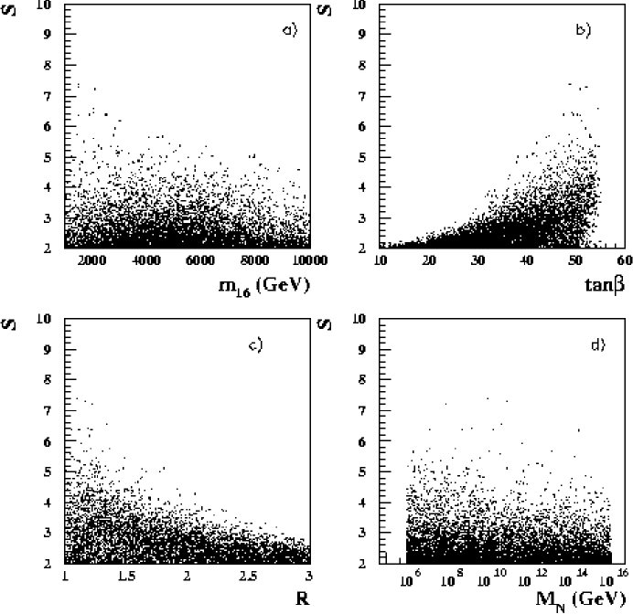
FIG. 1.: A plot of crunch factor $S$ versus a) $m_{16}$, b) $\tan\beta$, c) $R$ and d) $M_{N}$, for all models with $A_{0}<0$ and $\mu<0$.

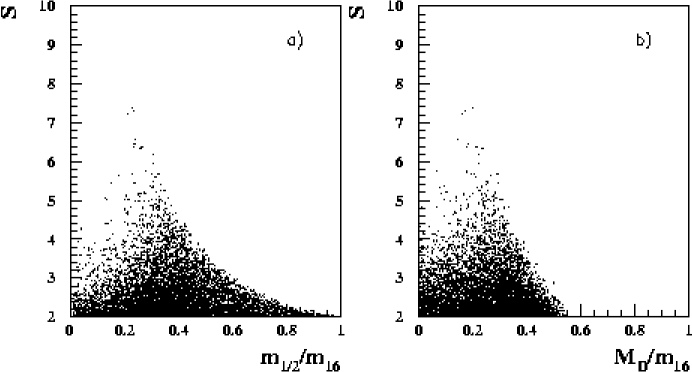
FIG. 2.: A plot of crunch factor $S$ versus a) $m_{1/2}/m_{16}$ and b) $M_{D}/m_{16}$, for all models with $A_{0}<0$ and $\mu<0$.

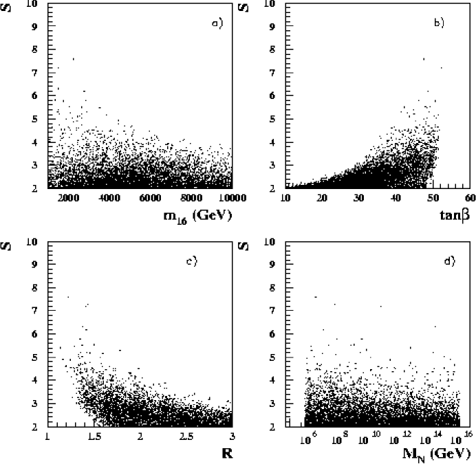
FIG. 3.: A plot of crunch factor $S$ versus a) $m_{16}$, b) $\tan\beta$, c) $R$ and d) $M_{N}$, for all models with $A_{0}<0$ and $\mu>0$.

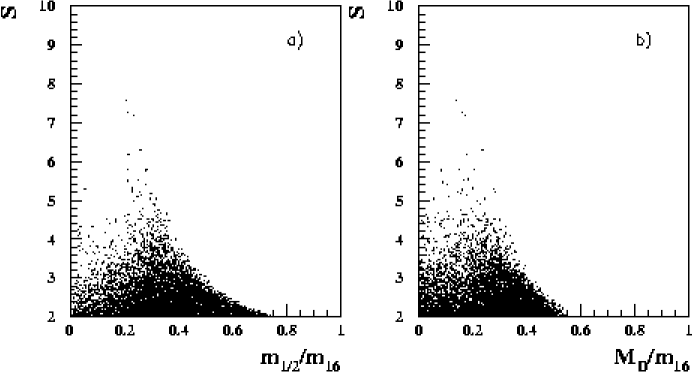
FIG. 4.: A plot of crunch factor $S$ versus a) $m_{1/2}/m_{16}$ and b) $M_{D}/m_{16}$, for all models with $A_{0}<0$ and $\mu>0$.

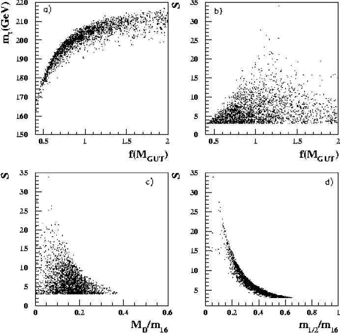
FIG. 5.: A plot of a) the physical value of $m_{t}$ versus $f(M_{GUT})$, b) crunch factor $S$ versus $f(M_{GUT})$, and c) $S$ versus $M_{D}/m_{16}$ and d) $S$ versus $m_{1/2}/m_{16}$, using a top-down solution to RGEs, and a unified $GUT$ scale Yukawa coupling. In these plots, we adopt $\mu<0$.

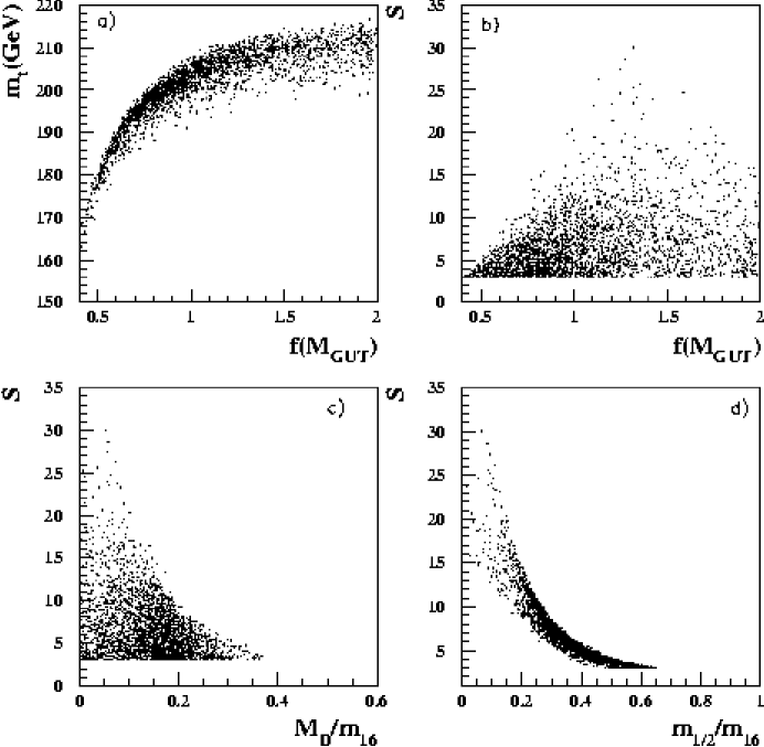
FIG. 6.: Same as Fig. 5, except for $\mu>0$.

FIG. 7.: A plot of allowed regions for the RIMH model in the $m_{16}\ vs.m_{1/2}$ plane, for $M_{N}=1\times 10^{7}$ GeV, $M_{D}=0.2m_{16}$, $\tan\beta=50$ and $\mu<0$. Points with triangles are excluded by a non-neutralino LSP, open circles by lack of REWSB and dots by tachyonic scalar masses. We show contours of $S=3$ and 5, $R=1.05$, $m_{\tilde{g}}=2$ TeV, $m_{\tilde{u}_{L}}=3$ TeV, $\mu=-1$ TeV, and $m_{\tilde{t}_{1}}$ and $m_{\tilde{b}_{1}}$ of 1 TeV. The stars denote points where bottom squarks should be detectable at the Fermilab Tevatron, assuming an integrated luminosity of 25 $fb^{-1}$.

FIG. 8.: A plot of a) $S$, b) $R$, c) $m_{\tilde{b}_{1}}$ and d) $m_{\tilde{t}_{1}}$ versus $m_{16}$ for $m_{1/2}=0.25m_{16}$, $\tan\beta=50$ and $\mu<0$, for the various $M_{N}$ values (in GeV) exhibited in the figure.

FIG. 9.: A plot of various sparticle and Higgs boson masses and $-\mu$ versus $m_{16}$ for $m_{1/2}=0.25m_{16}$, $\tan\beta=50$, $\mu<0$ and $M_{N}=1\times 10^{7}$ GeV.

FIG. 10.: Same as Fig. 7, except $\mu>0$. The degree of Yukawa unification ranges from $R=1.6-1.9$ thoughout the plane.

FIG. 11.: A plot of a) $S$, b) $R$, c) $m_{\tilde{b}_{1}}$ and d) $m_{\tilde{t}_{1}}$ versus $m_{16}$ for $m_{1/2}=0.22m_{16}$, $\tan\beta=50$ and $\mu>0$, for the various $M_{N}$ values (in GeV) exhibited in the figure.

FIG. 12.: A plot of various sparticle and Higgs boson masses and $\mu$ versus $m_{16}$ for $m_{1/2}=0.22m_{16}$, $\tan\beta=50$, $\mu>0$ and $M_{N}=1\times 10^{7}$ GeV.

FIG. 13.: The neutralino relic density as a function of $m_{16}$, for $M_{D}=0.2m_{16}$, $\tan\beta=50$, $M_{N}=1\times 10^{7}$ GeV and a) $\mu<0$ with $m_{1/2}=0.25m_{16}$ and b) $\mu>0$ with $m_{1/2}=0.22m_{16}$.

FIG. 14.: The branching fraction for the decay $b\rightarrow s\gamma$ for the same two slices of the parameter plane as in Fig. 13 versus the parameter $m_{16}$. The CLEO experiment requires that this branching fraction is between $2\times 10^{-4}$ and $4.5\times 10^{-4}$ at the 95% CL, while the recent measurement from the BELLE collaboration has a central value only slightly higher.

FIG. 15.: The Wilson coefficients a) $C_{7}$, and b) $C_{8}$ that enter the computation of the radiative decay of the $b$ quark, versus the model parameter $m_{16}$ for the parameter space slice with negative $\mu$. The dashed lines labelled, SM, $H^{\mp}$ and $\widetilde{W}$, respectively denote contributions to $C_{7}$ or $C_{8}$ from the SM $tW$ loop, the $tH^{+}$ loop and the $\widetilde{W}_{i}\tilde{q}_{j}$ loop. The sum of these is shown by the solid line labelled $C_{7,8}(M_{W})$. The result of evolving this down to the scale $m_{b}$ is shown as the other solid line labelled $C_{7,8}(m_{b})$.

FIG. 16.: The same as Fig. 15, except for the parameter space slice with $\mu>0$.

FIG. 17.: A plot of signal cross section over square root of background cross section for $0\ell$, $1\ell$, $OS$ and $SS$ dilepton events after cuts from the RIMH model at the CERN LHC, versus the parameter $m_{16}$. The $n-\sigma$ significance can be gained by multiplying by the square root of the integrated luminosity in fb. In a), we take $m_{1/2}=0.25m_{16}$ and $\mu<0$. In b), we take $m_{1/2}=0.22m_{16}$ and $\mu>0$. In both frames, we take $M_{D}=0.2m_{16}$, $\tan\beta=50$ and $M_{N}=1\times 10^{7}$ GeV.

FIG. 18.: A plot of signal cross section for multijet $+\not\!\!{E_{T}}$ events which contain exactly two tagged $b$-jets, after cuts, from the RIMH model at the CERN LHC, versus the parameter $m_{16}$. In a), we take $m_{1/2}=0.25m_{16}$ and $\mu<0$. In b), we take $m_{1/2}=0.22m_{16}$ and $\mu>0$. In both frames, we take $M_{D}=0.2m_{16}$, $\tan\beta=50$ and $M_{N}=1\times 10^{7}$ GeV.

REFERENCES

- [1] For recent reviews, see e.g. S. Martin, in Perspectives on Supersymmetry, edited by G. Kane (World Scientific), hep-ph/9709356; M. Drees, hep-ph/9611409 (1996); J. Bagger, hep-ph/9604232 (1996); X. Tata, Proc. IX J. Swieca Summer School, J. Barata, A. Malbousson and S. Novaes, Eds. hep-ph/9706307; S. Dawson, Proc. TASI 97, J. Bagger, Ed. hep-ph/9712464.
- [2] A. Chamseddine, R. Arnowitt and P. Nath, Phys. Rev. Lett. 49, 970 (1982); R. Barbieri, S. Ferrara and C. Savoy, Phys. Lett. B119, 343 (1982); L.J. Hall, J. Lykken and S. Weinberg, Phys. Rev. D27, 2359 (1983); for a review, see H. P. Nilles, Phys. Rep. 110, 1 (1984).
- [3] S. K. Soni and H. A. Weldon, Phys. Lett. B126, 215 (1983); V. Kaplunovsky and J. Louis, Phys. Lett. B306, 269 (1993).
- [4] F. Gabbiani, E. Gabrielli, A. Masiero and L. Silvestrini, Nucl. Phys. B477, 321 (1996).
- [5] K. Choi, J. S. Lee and C. Munoz, Phys. Rev. Lett. 80, 3686 (1998).
- [6] M. Dine, A. Nelson, Y. Nir and Y. Shirman, Phys. Rev. D53, 2658 (1996). For a review, see G. Giudice and R. Rattazzi, Phys. Rep. 322, 419 (1999).
- [7] L. Randall and R. Sundrum, Nucl. Phys. B557, 79 (1999); G. Giudice, M. Luty, H. Murayama and R. Rattazzi, JHEP 9812, 027 (1998).
- [8] M. Schmaltz and W. Skiba, Phys. Rev. D62 095004 (2000) and ibid D62 095005 (2000).
- [9] M. Dine, A. Kagan and S. Samuel, Phys. Lett. B243, 250 (1990).
- [10] See for example R. Barbieri and G. Giudice, Nucl. Phys. B306, 63 (1988); G. Anderson and D. Castano, Phys. Lett. B347, 300 (1995) and Phys. Rev. D52, 1693 (1995); S. Dimopoulos and G. Giudice, Phys. Lett. B357, 573 (1995); K. L. Chan, U. Chattopadhyay and P. Nath, Phys. Rev. D58, 096004 (1998).
- [11] M. Drees, Phys. Rev. D33, 1468 (1986); S. Dimopoulos and G. Giudice, Ref. [10]; A. Pomarol and D. Tommasini, Nucl. Phys. B466, 3 (1996); A.G. Cohen, D.B. Kaplan, and A.E. Nelson, Phys. Lett. B388, 588 (1996); J. Hisano, K. Kurosawa and Y. Nomura, Phys. Lett. B445, 316 (1999) and hep-ph/0002286 (2000); V. Barger, C. Kao and R-J. Zhang, Phys. Lett. B483, 184 (2000); for an overview, see H. Baer, M. Diaz, P. Quintana and X. Tata, JHEP 0004, 016 (2000).
- [12] N. Arkani-Hamed and H. Murayama, Phys. Rev. D56, R6733 (1997); K. Agashe and M. Graesser, Phys. Rev. D59, 015007 (1999).
- [13] H. Baer, C. Balázs, P. Mercadante, X. Tata and Y. Wang, Phys. Rev. D63, 015011 (2001).
- [14] J. Feng, C. Kolda and N. Polonsky, Nucl. Phys. B546, 3 (1999); J. Bagger, J. Feng and N. Polonsky, Nucl. Phys. B563, 3 (1999); J. Bagger, J. Feng, N. Polonsky and R. Zhang, Phys. Lett. B473, 264 (2000).
- [15] H. Baer, M. Diaz, J. Ferrandis and X. Tata, Phys. Rev. D61, 111701 (2000); H. Baer, M. Brhlik, M. Diaz, J. Ferrandis, P. Mercadante, P. Quintana and X. Tata, Phys. Rev. D63, 015007 (2001).
- [16] C. Kolda and S. Martin, Phys. Rev. D53, 3871 (1996); see references therein for a guide to the earlier literature.
- [17] H. Baer. P. Mercadante and X. Tata, Phys. Lett. B475, 289 (2000).
- [18] F. Paige, S. Protopopescu, H. Baer and X. Tata, hep-ph/0001086 (2000).
- [19] D. Pierce, J. Bagger, K. Matchev and R. Zhang, Nucl. Phys. B491, 3 (1997).
- [20] V. Barger, P. Ohmann and R. Phillips, Phys. Rev. D47, 1093 (1993); W. Bardeen, M. Carena, S. Pokorski and C.E.M. Wagner, Phys. Lett. B320, 110 (1994); M. Carena, M. Olechowski, S. Pokorski and C. Wagner, Nucl. Phys. B419, 213 (1994).
- [21] O. Yakovlev and S. Groote, hep-ph/0008156 (2000).
- [22] L.V. Avdeev and M. Yu. Kalmykov, Nucl. Phys. B502, 419 (1997).
- [23] H. Baer, P. Mercadante and X. Tata, Phys. Rev. D59, 015010 (1999).
- [24] H. Baer, M. Drees, R. Godbole, J. Gunion and X. Tata, Phys. Rev. D44, 725 (1991); H. Baer, J. Sender and X. Tata, Phys. Rev. D50, 4517 (1994); R. Demina, J. Lykken, K. Matchev and A. Nomerotski, Phys. Rev. D62, 035011 (2000); J. Sender, Ph. D. thesis, hep-ph/0010025 (2000).
- [25] H. Baer, V. Barger, D. Karatas and X. Tata, Phys. Rev. D36, 96 (1987).
- [26] H. Baer, C. H. Chen, F. Paige and X. Tata, Phys. Rev. D52, 2746 (1995) and Phys. Rev. D53, 6241 (1996); H. Baer, C. H. Chen, M. Drees, F. Paige and X. Tata, Phys. Rev. D59, 055014 (1999).
- [27] H. Baer and M. Brhlik, Phys. Rev. D53, 597 (1996) and Phys. Rev. D57, 567 (1998); V. Barger and C. Kao, Phys. Rev. D57, 3131 (1998).
- [28] P. Gondolo and G. Gelmini, Nucl. Phys. B360, 145 (1991).
- [29] K. Griest and D. Seckel, Phys. Rev. D43, 3191 (1991). J. Ellis, T. Falk, K. Olive and M. Srednicki, Astropart. Phys. 13, 181 (2000); C. Boehm, A. Djouadi and M. Drees, Phys. Rev. D62, 035012 (2000).
- [30] S. Ahmed et al. (CLEO Collaboration), hep-ex/9908022 (1999).
- [31] M. Nakao, presented at the International Conference on High Energy Physics, Osaka, Japan, July, 2000.
- [32] K. G. Chetyrkin, M. Misiak and M. Münz, Phys. Lett. B400, 206 (1997); A. Buras, A. Kwiatkowski and N. Pott, Phys. Lett. B414, 157 (1997); ibid., erratum, Phys. Lett. B434, 459 (1998); C. Grueb and T. Hurth, hep-ph9708214 (1997).
- [33] H. Baer and M. Brhlik, Phys. Rev. D55, 3201 (1997); H. Baer, M. Brhlik, D. Castano and X. Tata, Phys. Rev. D58, 015007 (1998). See references cited herein for a guide to the original computations of these decays.
- [34] M. Carena and C. Wagner, CERN-TH-7321-94 (1994); F. Borzumati, M. Olechowski and S. Pokorski, Phys. Lett. B349, 311 (1995).
- [35] S. Abel et al. (SUGRA Working Group Collaboration, Fermilab Run 2 Workshop), hep-ph/0003154 (2000).
- [36] S. Martin and M. Vaughn, Phys. Rev. D50, 2282 (1994).
- [37] V. Barger, M. Berger and P. Ohmann, Phys. Rev. D49, 4908 (1994).