Minimisation of a one-loop charge breaking effective potential

Abstract. We compute the field derivatives of a one-loop charge breaking effective potential and analyse their effect in its minimisation. The impact on charge breaking bounds on the MSSM parameters is discussed.

DIAS-STP-01-03

Spontaneous gauge symmetry breaking occurs in the Minimal Supersymmetric Standard Model when the neutral - and obviously colourless - components of the Higgs doublets $H_{1}$ and $H_{2}$ acquire non zero vevs. The presence in the theory of many other scalar fields means there is no a priori reason why the minimum of the potential should be a charge and colour preserving one. If fields other than $H_{1}^{0}$ and $H_{2}^{0}$ have vevs and for a particular combination of MSSM parameters the resulting minimum is deeper than the standard one we would therefore be in a situation where charge and/or colour symmetries were broken. This simple fact gives us, in principle, a way of imposing bounds on the MSSM parameter space [1]. There has been a great deal of work done in this area [2], most of it based on the analysis of the tree-level effective potential along specific charge and/or colour breaking (CCB) directions. A fundamental point in these works is that the CCB and MSSM potentials be compared at different renormalisation scales - this is based upon the work of Gamberini et al [3], where it was showed the vevs derived from the tree-level MSSM potential are a reasonable approximation to those obtained from the one-loop potential if one chooses a renormalisation scale of the order of the largest particle mass in the theory. Because that typical mass is different in the MSSM (of the order of tens or hundreds of GeV) and the CCB (of the TeV or tens of TeV order) cases, comparing both potentials at the tree-level order should in principle be done at two different scales. The authors of ref. [4] determined CCB bounds including the one-loop contributions to the potential from the top-stop sectors, which they argued were the most significant ones. Recently [5] the full one-loop potential for a particular CCB direction was calculated and used to restrict the parameter space of the MSSM. It was argued that comparing the MSSM and CCB potentials at different renormalisation scales neglected to take into account the field-independent part of those same potentials, vital to ensure their renormalisation group invariance [6]. The higgs and chargino contributions to the one-loop potential proved to be as important as the top-stop ones. This analysis was done at the typical CCB mass scale, so that, using the results of [3], the computation of the one-loop derivatives of the CCB potential could be avoided. The results that were found had some renormalisation scale dependence, and it was then theorised that it would vanish if one performed the full one-loop minimisation of the CCB potential. In this letter we will undertake just that task. We rely heavily on the results of ref. [5] and refer the reader to its conventions. We recall that we only consider the Yukawa couplings of the third generation, and the superpotential of the model is thus given by

$$W = \lambda_{t}H_{2}\,Q\,t_{R}\;+\;\lambda_{b}H_{1}\,Q\,b_{R}\;+\;\lambda_{\tau}H_{1}\,L\,\tau_{R}\;+\;\mu H_{2}\,H_{1}\;\;\;.$$ (1)

Supersymmetry is broken softly in the standard manner by the inclusion in the potential of explicit mass terms for the scalar partners and gauginos, and soft-breaking bilinear and trilinear terms proportional, via coefficients $A_{i}$ and $B$, to their counterparts in the superpotential (1). At a renormalisation scale $M$, the one-loop contributions to the potential are given by

$$\Delta V_{1}\,=\,\sum_{\alpha}\,\frac{n_{\alpha}}{64\pi^{2}}\,M_{\alpha}^{4}\,\left(\,\log\frac{M_{\alpha}^{2}}{M^{2}}\,-\,\frac{3}{2}\,\right)\;\;\;,$$ (2)

where the $M_{\alpha}$ are the tree-level masses of each particle of spin $s_{\alpha}$ and $n_{\alpha}=(-1)^{2s_{\alpha}}\,(2s_{\alpha}+1)\,C_{\alpha}\,Q_{\alpha}$. $C_{\alpha}$ is the number of colour degrees of freedom and $Q_{\alpha}$ is 2 for charged particles, 1 for chargeless ones. The “real” minimum occurs when the neutral components of $H_{1}$ and $H_{2}$ acquire vevs $v_{1}/\sqrt{2}$ and $v_{2}/\sqrt{2}$, the value of the tree-level potential then being

$$V_{0}\;=\;\frac{1}{2}\left(m_{1}^{2}\,v_{1}^{2}\;+\;m_{2}^{2}\,v_{2}^{2}\right)\;-\;B\,\mu\,v_{1}\,v_{2}\;+\;\frac{1}{32}({g^{\prime}}^{2}+g_{2}^{2})\,(v_{2}^{2}-v_{1}^{2})^{2}\;\;\;,$$ (3)

with $m_{1}^{2}=m_{H_{1}}^{2}+\mu^{2}$ and $m_{2}^{2}=m_{H_{2}}^{2}+\mu^{2}$. In the CCB direction we will consider the scalar fields $\tau_{L}$ and $\tau_{R}$ also have non-zero vevs, $l/\sqrt{2}$ and $\tau/\sqrt{2}$ respectively, and the vacuum tree-level potential is now given by

$$V_{0} = \frac{\lambda_{\tau}^{2}}{4}[v_{1}^{2}\,(l^{2}+\tau^{2})+l^{2}\,\tau^{2}]\;-\;\frac{\lambda_{\tau}}{\sqrt{2}}\,(A_{\tau}\,v_{1}+\mu\,v_{2})\,l\,\tau\;+\;\frac{1}{2}\,(m_{1}^{2}\,v_{1}^{2}\;+\;m_{2}^{2}\,v_{2}^{2}\;+\;m_{L}^{2}\,l^{2}\;+$$ (4)

$$m_{\tau}^{2}\,\tau^{2})\;-\;B\,\mu\,v_{1}\,v_{2}\;+\;\frac{g^{\prime 2}}{32}\,(v_{2}^{2}-v_{1}^{2}-l^{2}+2\,\tau^{2})^{2}\;+\;\frac{g_{2}^{2}}{32}\,(v_{2}^{2}-v_{1}^{2}+l^{2})^{2}\;\;\;.$$

The derivatives of this tree-level potential with respect to each of the vevs are very simple, but the same cannot be said for the one-loop derivatives, their total contribution given by

$$\sum_{\alpha}\,\frac{n_{\alpha}}{32\pi^{2}}\,M_{\alpha}^{2}\,\frac{\partial M_{\alpha}^{2}}{\partial v_{i}}\,\left(\,\log\frac{M_{\alpha}^{2}}{M^{2}}\,-\,1\,\right)\;\;\;.$$ (5)

Some of the squared masses’ derivatives are trivial to calculate: that is the case of the top and bottom quarks, and the scalar partners of the second and first generation up and down quarks and electron and neutrinos (expressions (15) to (18) of ref. [5]) - we present these results in the appendix. For the remaining sparticles the calculation is made more difficult by the masses being given by the eigenvalues of square matrices, sometimes as large as $6\times 6$ - many of these matrices are much more complex than their MSSM counterparts due to the existence of charged vevs causing mixing of charged and neutral fields. For example, the “higgs scalars” of the CCB potential are in fact the result of the mixing between the neutral components of $H_{1}$, $H_{2}$ and the fields $\tau_{L}$ and $\tau_{R}$, their squared masses thus given by the eigenvalues of a $4\times 4$ matrix. It is nevertheless possible to find analytical expressions for $\partial M_{\alpha}^{2}/\partial v_{i}$, once the $M_{\alpha}$ themselves have been determined (which is easy to do numerically, where an analytical determination proves impossible) - this is accomplished by noticing that the particle masses are always given by the roots of an $n^{th}$-order polynomial (in our case, $n=2$, 3, 4 and 6),

$$F(\lambda\;,\;v_{i})\;=\;\lambda^{n}\;+\;A\,\lambda^{n-1}\;+\;B\,\lambda^{n-2}\;+\;\ldots\;=\;0\;\;\;,$$ (6)

with coefficients $\{A,B,\ldots\}$ generally depending on the vevs $v_{i}=\{v_{1},v_{2},l,\tau\}$. This equation implicitly defines the squared masses $\lambda$ in function of the $v_{i}$, so we have

$$\frac{\partial M_{\alpha}^{2}}{\partial v_{i}}\;=\;-\;\left.\frac{{\displaystyle\frac{\partial F}{\partial v_{i}}}}{{\displaystyle\frac{\partial F}{\partial\lambda}}}\;=\;-\;\frac{{\displaystyle\frac{\partial A}{\partial v_{i}}}\,\lambda^{n-1}\;+\;{\displaystyle\frac{\partial B}{\partial v_{i}}}\,\lambda^{n-2}\;+\;\ldots}{n\,\lambda^{n-1}\;+\;(n-1)\,A\,\lambda^{n-2}\;+\;(n-2)\,B\,\lambda^{n-3}\;+\;\ldots}\;\;\right|_{\lambda=M_{\alpha}^{2}}\;\;\;.$$ (7)

If $n>2$ the final expressions depend on the numerical solving of eq. (6). For $n=2$ it is possible to write down fully analytical expressions of the derivatives of the squared masses, but from a practical point of view it is better to use the recipe of eq. (7). In the following we show how to calculate the coefficients $\{A,B,C,\ldots\}$ (and their derivatives) of eq. (6) for the several sparticles in terms of the elements $\{a,b,c,\ldots\}$ of their mass matrices. The derivatives of $\{a,b,c,\ldots\}$ are listed in the appendix. So, for a symmetric $2\times 2$ mass matrix with diagonal elements $a$ and $c$ and off-diagonal element $b$, eq. (7) reduces to

$$\frac{\partial M_{\alpha}^{2}}{\partial v_{i}}\;=\;\frac{a\,{\displaystyle\frac{\partial c}{\partial v_{i}}}\;+\;c\,{\displaystyle\frac{\partial(ac)}{\partial v_{i}}}\;-\;2\,b\,{\displaystyle\frac{\partial b}{\partial v_{i}}}\;-\;{\displaystyle\frac{\partial(a\,+\,c)}{\partial v_{i}}}}{a\;+\;c\;-\;2\,\lambda}\;\;\;.$$ (8)

This is the case of the stop, sbottom and neutral gauge boson masses, the coefficients $\{a,b,c\}$ are given in eqs. (12), (14) and (21) of ref. [5], and their derivatives a simple calculation. The squared masses of the charginos are also determined by a quadratic equation , namely (from eq. (22) of ref. [5]), $\lambda^{2}\;-\;A_{\chi^{\pm}}\,\lambda\;+\;B_{\chi^{\pm}}\;=\;0$, with

$$A_{\chi^{\pm}} = M_{2}\;+\;\mu^{2}\;+\;\frac{1}{2}\,\left[g_{2}^{2}\,(v_{1}^{2}+v_{2}^{2}+l^{2})\;+\;\lambda_{\tau}^{2}\,\tau^{2}\right]$$

$$B_{\chi^{\pm}} = \left(\frac{1}{2}\,g_{2}^{2}\,v_{1}\,v_{2}\;-\;\mu\,M_{2}\right)^{2}\;+\;\frac{1}{2}\,g_{2}^{2}\,l^{2}\,\left(\frac{1}{2}\,g_{2}^{2}\,v_{1}^{2}\;+\;\mu^{2}\right)\;+\;\frac{\lambda_{\tau}^{2}}{2}\,\left(\frac{1}{2}\,g_{2}^{2}\,v_{2}^{2}\;+\;M_{2}^{2}\right)\,\tau^{2}\;-$$ (9)

$$\frac{\lambda_{\tau}}{\sqrt{2}}\,g_{2}^{2}\,(\mu\,v_{2}\;+\;M_{2}\,v_{1})\,l\,\tau\;\;\;.$$

All that remains is to calculate the derivatives of $A_{\chi^{\pm}}$ and $B_{\chi^{\pm}}$ and substitute their values in eq. (7). The charged Higgses are a mix between the charged components of $H_{1}$ and $H_{2}$ and the tau sneutrino, with a $3\times 3$ mass matrix with elements $\{a_{\pm},b_{\pm},\ldots,f_{\pm}\}$, as shown in eq. (24) of ref. [5]. The squared masses end up being determined by a cubic equation,

$$\lambda^{3}\;-\;A_{\pm}\,\lambda^{2}\;-\;B_{\pm}\,\lambda\;-\;C_{\pm}\;=\;0\;\;\;,$$ (10)

with

$$A_{\pm} = a_{\pm}\;+\;c_{\pm}\;+\;f_{\pm}$$

$$B_{\pm} = b_{\pm}^{2}\;+\;d_{\pm}^{2}\;+\;e_{\pm}^{2}\;-\;a_{\pm}\,(c_{\pm}+f_{\pm})\;-\;c_{\pm}\,f_{\pm}\;\;\;.$$ (11)

$C_{\pm}$ is, of course, the determinant of the mass matrix, but we end up not needing to calculate it, only its derivative. Adopting the convention $X_{,v}$ to indicate $\partial X/\partial v$, with $v$ any of the vevs, we obtain

$$A_{\pm,v} = a_{\pm,v}\;+\;c_{\pm,v}\;+\;f_{\pm,v}$$

$$B_{\pm,v} = 2\,(b_{\pm}\,b_{\pm,v}\;+\;d_{\pm}\,d_{\pm,v}\;+\;e_{\pm}\,{}_{\pm}\,e_{\pm,v})\;-\;a_{\pm}\,(c_{\pm,v}\;+\;f_{\pm,v})\;-\;c_{\pm}\,(a_{\pm,v}\;+\;f_{\pm,v})\;-$$

$$f_{\pm}\,(a_{\pm,v}\;+\;c_{\pm,v})$$

$$C_{\pm,v} = 2\,(b_{\pm,v}\,d_{\pm}\,e_{\pm}\;+\;d_{\pm,v}\,b_{\pm}\,e_{\pm}\;+\;e_{\pm,v}\,b_{\pm}\,d_{\pm})\;+\;a_{\pm,v}\,c_{\pm}\,f_{\pm}\;+\;c_{\pm,v}\,a_{\pm}\,f_{\pm}\;+$$ (12)

$$f_{\pm,v}\,a_{\pm}\,c_{\pm}\;-\;d_{\pm}\,(2\,d_{\pm,v}\,c_{\pm}\;+\;c_{\pm,v}\,d_{\pm})\;-\;b_{\pm}\,(2\,b_{\pm,v}\,f_{\pm}\;+\;f_{\pm,v}\,b_{\pm})\;-$$

$$e_{\pm}\,(2\,e_{\pm,v}\,a_{\pm}\;+\;a_{\pm,v}\,e_{\pm})\;\;\;.$$

The squared masses of both the pseudoscalars and Higgs scalars are given by $4\times 4$ matrices (eqs. (26) and (28) of ref. [5]) with one set of coefficients $\{a,b,\ldots j\}$ for each case. The resulting fourth-order eigenvalue equation,

$$\lambda^{4}\;-\;A\,\lambda^{3}\;+\;B\,\lambda^{2}\;+\;C\,\lambda\;+\;D\;=\;0\;\;\;,$$ (13)

has coefficients

$$A = a\;+\;c\;+\;h\;+\;j$$

$$B = a\,(c\;+\;h\;+\;j)\;+\;c\,(h\;+\;j)\;+\;h\,j\;-\;b^{2}\;-\;d^{2}\;-\;e^{2}-\;f^{2}\;-\;g^{2}-\;i^{2}$$

$$C = a\,(g^{2}\;+\;f^{2}\;+\;i^{2}\;-\;c\,j\;-\;c\,h\;-\;h\,j)\;+\;c\,(d^{2}\;+\;e^{2}\;+\;i^{2}\;-\;h\,j)\;+$$ (14)

$$h\,(b^{2}\;+\;e^{2}\;+\;g^{2})\;+\;j\,(b^{2}\;+\;d^{2}\;+\;f^{2})\;-$$

$$2\,(f\,g\,i\;+\;b\,f\,d\;+\;d\,e\,i\;+\;b\,g\,e)\;\;\;.$$

Once again, for the calculation of the derivatives of eq. (7), we don’t need the explicit value of $D$, the determinant of the mass matrix. With the same convention as before, we have

$$A_{,v} = a_{,v}\;+\;c_{,v}\;+\;h_{,v}\;+\;j_{,v}$$

$$B_{,v} = a\,(c_{,v}\;+\;h_{,v}\;+\;j_{,v})\;+\;c\,(a_{,v}\;+\;h_{,v}\;+\;j_{,v})\;+\;h\,(a_{,v}\;+\;c_{,v}\;+\;j_{,v})\;+$$

$$j\,(a_{,v}\;+\;c_{,v}\;+\;h_{,v})\;-\;2\,(b\,b_{,v}\;+\;d\,d_{,v}\;+\;e\,e_{,v}\;+\;f\,f_{,v}\;+\;g\,g_{,v}\;+\;i\,i_{,v})$$

$$C_{,v} = a_{,v}\,(g^{2}\,+\,f^{2}\,+\,i^{2}\,-\,c\,j\,-\,c\,h\,-\,h\,j)\,+\,c_{,v}\,(d^{2}\,+\,e^{2}\,+\,i^{2}\,-\,a\,j\,-\,a\,h\,-\,h\,j)\,+$$

$$h_{,v}\,(b^{2}\,+\,e^{2}\,+\,g^{2}-\,a\,j\,-\,a\,c\,-\,c\,j)\,+\,j_{,v}\,(b^{2}\,+\,d^{2}\,+\,f^{2}-\,a\,h\,-\,a\,c\,-\,c\,h)\,+$$

$$2\,b_{,v}\,(b\,h\,+\,b\,f\,-\,f\,d\,-\,g\,e)\,+\,2\,d_{,v}\,(d\,c\,+\,d\,j\,-\,b\,f\,-\,e\,i)\,+$$

$$2\,e_{,v}\,(e\,c\,+\,e\,h\,-\,d\,i\,-\,b\,g)\,+\,2\,f_{,v}\,(f\,a\,+\,f\,j\,-\,g\,i\,-\,b\,d)\,+$$

$$2\,g_{,v}\,(g\,a\,+\,g\,h\,-\,f\,i\,-\,e\,b)\,+\,2\,i_{,v}\,(i\,a\,+\,i\,c\,-\,g\,f\,-\,e\,d)$$

$$D_{,v} = a_{,v}\,(chj+2\,fgi-jf^{2}-ci^{2}-hg^{2})\,+\,c_{,v}\,(ahj+2\,dei-jd^{2}-ai^{2}-he^{2})\,+$$ (15)

$$h_{,v}\,(acj+2\,beg-jb^{2}-ag^{2}-ce^{2})\,+\,j_{,v}\,(ach+2\,bfd-hb^{2}-af^{2}-cd^{2})\,+$$

$$2\,b_{,v}\,(b\,i^{2}\,-\,b\,h\,j\,+\,f\,d\,j\,+\,g\,e\,h\,-\,f\,e\,i\,-\,g\,d\,i)\,+$$

$$2\,d_{,v}\,(d\,g^{2}\,-\,c\,d\,j\,+\,f\,b\,j\,+\,c\,e\,i\,-\,b\,g\,i\,-\,e\,g\,f)\,+$$

$$2\,e_{,v}\,(e\,f^{2}\,-\,c\,h\,e\,+\,g\,b\,h\,+\,c\,d\,i\,-\,b\,f\,i\,-\,g\,d\,f)\,+$$

$$2\,f_{,v}\,(f\,e^{2}\,-\,a\,f\,j\,+\,d\,b\,j\,+\,a\,g\,i\,-\,b\,e\,i\,-\,g\,d\,e)\,+$$

$$2\,g_{,v}\,(g\,d^{2}\,-\,a\,h\,g\,+\,e\,b\,h\,+\,a\,f\,i\,-\,b\,d\,i\,-\,f\,d\,e)\,+$$

$$2\,i_{,v}\,(i\,b^{2}\,-\,a\,c\,i\,+\,a\,f\,g\,+\,d\,c\,e\,-\,b\,f\,e\,-\,b\,d\,g)$$

For the neutralinos, the sixth-order equation for the masses is made reasonably simple by the mass matrix (eq. (23) of [5]) having several zeroes. We thus have

$$\lambda^{6}\;-\;A_{\chi^{0}}\,\lambda^{5}\;-\;B_{\chi^{0}}\,\lambda^{4}\;+\;C_{\chi^{0}}\,\lambda^{3}\;+\;D_{\chi^{0}}\,\lambda^{2}\;+\;E_{\chi^{0}}\,\lambda\;+\;F_{\chi^{0}}\,\lambda\;=\;0\;\;\;,$$ (16)

with

$$A_{\chi^{0}} = M_{1}\,+\,M_{2}$$

$$B_{\chi^{0}} = \frac{\lambda_{\tau}^{2}}{2}\,(v_{1}^{2}\,+\,l^{2}\,+\,\tau^{2})\;+\;\frac{1}{4}\,({g^{\prime}}^{2}\,+\,g_{2}^{2})\,(v_{1}^{2}\,+\,v_{2}^{2}\,+\,l^{2})\;+\;{g^{\prime}}^{2}\,\tau^{2}\;+\;\mu^{2}\;-\;M_{1}\,M_{2}$$

$$C_{\chi^{0}} = -\,\frac{\lambda_{\tau}^{2}}{2}\,(M_{1}\,+M_{2})\,(v_{1}^{2}\,+\,l^{2}\,+\,\tau^{2})\;-\;\frac{1}{4}\,({g^{\prime}}^{2}\,M_{2}\,+\,g_{2}^{2}\,M_{1})\,(v_{1}^{2}\,+\,v_{2}^{2}\,+\,l^{2})\;-$$

$${g^{\prime}}^{2}\,M_{2}\,\tau^{2}\;+\;\frac{1}{2}\,({g^{\prime}}^{2}\,+\,g_{2}^{2})\,\mu\,v_{1}\,v_{2}\;-\;\frac{\lambda_{\tau}}{2\sqrt{2}}\,(3\,{g^{\prime}}^{2}\,-\,g_{2}^{2}\,-\,2\,\lambda_{\tau}^{2})\,v_{1}\,l\,\tau\;-\;\mu^{2}\,(M_{1}\,+\,M_{2})$$

$$D_{\chi^{0}} = \frac{\lambda_{\tau}^{3}}{\sqrt{2}}\,(M_{1}\,+\,M_{2})\,v_{1}\,l\,\tau\;+\;\lambda_{\tau}^{2}\,\left\{\frac{}{}\right.\frac{{g^{\prime}}^{2}}{2}\,\tau^{2}\,(v_{1}^{2}\,+\,l^{2}\,+\,\tau^{2})\;+\;\frac{1}{8}\,({g^{\prime}}^{2}\,+\,g_{2}^{2})\,\left[v_{1}^{4}\,+\,l^{4}\,+\right.$$

$$\left.l^{2}\,(v_{2}^{2}\,-\,2\,v_{1}^{2})\,+\,v_{2}^{2}\,(v_{1}^{2}\,+\,\tau^{2})\right]\;-\;\frac{1}{2}\,M_{1}\,M_{2}\,(v_{1}^{2}\,+\,l^{2}\,+\,\tau^{2})\,+\frac{\mu^{2}}{2}\,v_{1}^{2}\left.\frac{}{}\right\}\;+$$

$$\frac{\lambda_{\tau}}{2\sqrt{2}}\,l\,\tau\,\left[(g_{2}^{2}\,M_{1}\,-\,3\,{g^{\prime}}^{2}\,M_{2})\,v_{1}\;+\;({g^{\prime}}^{2}\,-\,g_{2}^{2})\,\mu\,v_{2}\right]\;+$$

$$\frac{1}{4}\,{g^{\prime}}^{2}\,g_{2}^{2}\,(v_{1}^{2}\,+\,v_{2}^{2}\,+\,l^{2})\,\tau^{2}\;+\;\frac{1}{2}\,({g^{\prime}}^{2}\,M_{2}\,+\,g_{2}^{2}\,M_{1})\,\mu\,v_{1}\,v_{2}\;+$$

$$\left[\frac{1}{4}\,({g^{\prime}}^{2}\,+\,g_{2}^{2})\,l^{2}\;+\;{g^{\prime}}^{2}\,\tau^{2}\;-\;\,M_{1}\,M_{2}\right]\,\mu^{2}$$

$$E_{\chi^{0}} = \frac{\lambda_{\tau}^{3}}{\sqrt{2}}\,\left[\frac{1}{4}\,({g^{\prime}}^{2}\,+\,g_{2}^{2})\,v_{2}^{2}\;-\;M_{1}\,M_{2}\right]\,v_{1}\,l\,\tau\;+\;\lambda_{\tau}^{2}\,\left\{\frac{}{}\right.-\,\frac{1}{8}\,({g^{\prime}}^{2}\,M_{2}\,+\,g_{2}^{2}\,M_{1})\,\left[v_{1}^{4}\,+\,l^{4}\,+\right.$$

$$\left.l^{2}\,(v_{2}^{2}\,-\,2\,v_{1}^{2})\,+\,v_{2}^{2}\,(v_{1}^{2}\,+\,\tau^{2})\right]\;-\;\frac{1}{4}\,({g^{\prime}}^{2}\,+\,g_{2}^{2})\,\mu\,v_{1}\,v_{2}\,(l^{2}\,-\,v_{1}^{2})\;-$$

$$\frac{\mu^{2}}{2}\,(M_{1}\,+\,M_{2})\,v_{1}^{2}\;-\;\frac{{g^{\prime}}^{2}}{2}\,\tau^{2}\,\left[M_{2}\,(v_{1}^{2}\,+\,l^{2}\,+\,\tau^{2})\;-\;\mu\,v_{1}\,v_{2}\right]\left.\frac{}{}\right\}\;+$$

$$\frac{\lambda_{\tau}}{2\sqrt{2}}\,l\,\tau\,\left[{g^{\prime}}^{2}\,(g_{2}^{2}\,\tau^{2}\;-\;2\,\mu^{2})\,v_{1}\;+\;(g_{2}^{2}\,M_{1}\,-\,{g^{\prime}}^{2}\,M_{2})\,\mu\,v_{2}\right]\;-$$

$$\frac{1}{4}\,({g^{\prime}}^{2}\,M_{2}\,+\,g_{2}^{2}\,M_{1})\,\mu^{2}\,l^{2}\;+\;\frac{{g^{\prime}}^{2}}{2}\,(g_{2}^{2}\,v_{1}\,v_{2}\;-\;2\,\mu\,M_{2})\,\mu\,\tau^{2}$$

$$F_{\chi^{0}} = -\,\frac{\lambda_{\tau}^{3}}{4\sqrt{2}}\,({g^{\prime}}^{2}\,M_{2}\,+\,g_{2}^{2}\,M_{1})\,v_{1}\,l\,\tau\,v_{2}^{2}\;+\;\frac{\lambda_{\tau}^{2}}{4}\,\left[({g^{\prime}}^{2}\,M_{2}\,+\,g_{2}^{2}\,M_{1})\,\mu\,(l^{2}\,-\,v_{1}^{2})\,v_{1}\,v_{2}\;+\frac{}{}\right.$$ (17)

$$\left.2\,\mu^{2}\,M_{1}\,M_{2}\,v_{1}^{2}\;-\;\frac{{g^{\prime}}^{2}}{2}\,v_{2}\,\tau^{2}\,(4\,\mu\,M_{2}\,v_{1}\;+\;g_{2}^{2}\,\tau^{2}\,v_{2})\right]\;+$$

$$\frac{\lambda_{\tau}}{2\sqrt{2}}\,{g^{\prime}}^{2}\,(2\,\mu\,M_{2}\,v_{1}\;+\;g_{2}^{2}\,\tau^{2}\,v_{2})\,\mu\,l\,\tau\;-\;\frac{\mu^{2}}{4}\,{g^{\prime}}^{2}\,g_{2}^{2}\,l^{2}\,\tau^{2}\;\;\;.$$

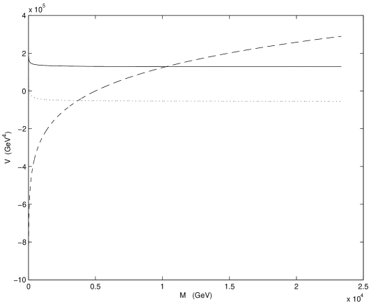
Figure 1: Evolution of $(V_{0}\,+\,\Delta V_{1})^{CCB}(v_{i}^{1})$, $(V_{0}\,+\,\Delta V_{1})^{CCB}(v_{i}^{0})/100$ and $(V_{0}\,+\,\Delta V_{1})^{MSSM}$ (solid, dashed and dotted lines respectively) with the renormalisation scale $M$. Notice how the two one-loop minimised potentials run almost parallel to one another. For this case, $M_{G}=$ 80 GeV, $m_{G}=$ 40 GeV, $A_{G}=$ 400 GeV, $\tan\beta=$ 6.5 and $\mu_{G}=$ -1.436.

With such complex formulae, a check of the results is quite useful - because supersymmetry is softly broken, $Str\,M^{2}$ is a field-independent quantity, so we should have $Str\,\partial M^{2}/\partial v_{i}\,=\,0$. In this manner we can check the mass matrices themselves  and the consistency of our sign conventions. With the derivatives (5) computed, we can perform the one-loop minimisation of the CCB potential. We apply our formulae to the same simple model of ref. [5]: one with universality of the soft parameters at the gauge unification scale and input parameters in the ranges $20\leq M_{G}\leq 100$ GeV, $10\leq m_{G}\leq 160$ GeV, $-600\leq A_{G}\leq 600$ GeV and $2.5\leq\tan\beta\leq 10.5$, with both signs of the $\mu$ parameter considered. In the work of ref. [5], we had performed the tree-level minimisation of the CCB potential at a renormalisation scale $M=0.6\,g_{2}|A_{\tau}|/\lambda_{\tau}$ - which was shown to be of the order of the highest of the CCB masses - and, out of an initial parameter space of about 3200 “points”, CCB extrema had been found for roughly $40\%$ of the cases. However, by repeating the process with the full one-loop derivatives of the CCB potential, we encounter drastically different results - only in almost 200 “points” does CCB seem to occur. These “points” are uniformly distributed according to the input parameters of $M_{G}$ and $m_{G}$, do not occur for values of $\mu_{G}$ close to zero (like in ref. [5]) and occur mostly for $\tan\beta>$ 6 and $150<|A_{G}|<500$ GeV. In figure (1) we see the reason for the discrepancy between these results and those of ref. [5]: there we have plotted the evolution with the renormalisation scale $M$ of the value of the one-loop MSSM potential ($(V_{0}+\Delta V_{1})^{MSSM}$, with one-loop vevs) and the one-loop CCB potentials calculated with the tree-level CCB vevs ($(V_{0}+\Delta V_{1})^{CCB}(v_{i}^{0})$ - for convenience, we divide it by a factor of 100) and the one-loop derived vevs ($(V_{0}+\Delta V_{1})^{CCB}(v_{i}^{1})$). To interpret this figure, we need to remember that $V_{0}+\Delta V_{1}$ is not a one-loop renormalisation scale independent quantity [6], rather, in terms of the parameters $\lambda_{i}$ and fields $\phi_{j}$, the RGE invariant effective potential is given by

$$V(M,\lambda_{i},\phi_{j})\;=\;\Omega(M,\lambda_{i})\;+\;V_{0}(\lambda_{i},\phi_{j})\;+\;\Delta V_{1}(M,\lambda_{i},\phi_{j})\;+\;O(\hbar^{2})\;\;\;.$$ (18)

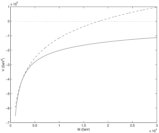
Figure 2: Evolution of $(V_{0}\,+\,\Delta V_{1})^{CCB}(v_{i}^{1})$, $(V_{0}\,+\,\Delta V_{1})^{CCB}(v_{i}^{0})$ and $(V_{0}\,+\,\Delta V_{1})^{MSSM}$ (solid, dashed and dotted lines respectively) with the renormalisation scale $M$. The strong variation with $M$ of the vevs displayed in fig. (3) causes the similar dependence of the CCB potential here. $M_{G}=$ 100 GeV, $m_{G}=$ 160 GeV, $A_{G}=$ -600 GeV, $\tan\beta=$ 10.5 and $\mu_{G}=$ -2.9823.

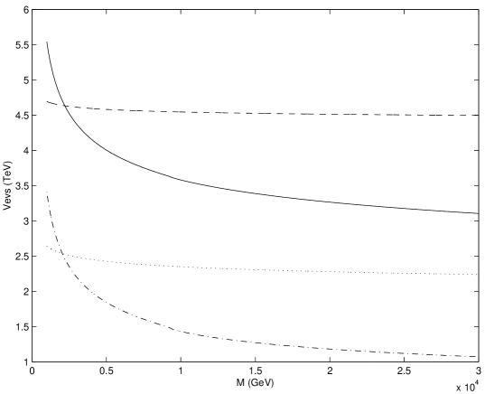
Figure 3: Evolution of the vevs $v_{1}$ (from one-loop - solid line - and tree-level - dashed line - minimisation) and $v_{2}$ (from one-loop - dot-dashed line - and tree-level - dotted line - minimisation) with the renormalisation scale $M$, for the same choice of parameters of fig. (2). Notice the large difference in value between the tree-level and one-loop vevs. For very high values of the renormalisation scale, the one-loop vevs begin to stabilise.

The only difference between the CCB and MSSM potentials is the different set of values for some of the fields $\phi_{j}$, which means the field-independent function $\Omega$ is the same in both cases . Therefore, given that $V$ is renormalisation scale invariant, we must have $d(V_{0}+\Delta V_{1})^{CCB}/dM\;=\;d(V_{0}+\Delta V_{1})^{MSSM}/dM$ - this is certainly the case for the two one-loop minimised potentials of fig. (1) (a plot of their renormalisation scale derivatives would show them to be almost identical for $M\gtrsim 1$ TeV), as they run parallel to one another, but the one-loop potential calculated with the tree-level vevs is clearly different. It has a very strong $M$ dependence, and the inequality $(V_{0}+\Delta V_{1})^{CCB}(v_{i}^{0})\,<\,(V_{0}+\Delta V_{1})^{MSSM}$ is verified only for $M\lesssim 4$ TeV. Notice how, judging by the value of the one-loop minimised CCB potential, this “point” is not a CCB minimum. Unfortunately, we find that for those points that are identified as one-loop CCB minima the potential does not have the correct renormalisation scale dependence seen in fig. (1), as may be seen in fig. (2) - there, for a different choice of parameters, we obtain CCB potentials that, whether computed with tree-level or one-loop vevs, are strongly dependent on $M$. Although the one-loop vevs do seem to somewhat stabilize $(V_{0}+\Delta V_{1})^{CCB}$, one can expect its value will become greater than the MSSM potential for a higher renormalisation scale. Again, the finding of a CCB minimum becomes $M$-dependent. The reason for this seems to be the values of the vevs found - in the case of fig. (1) the one-loop vevs are smaller than 1 TeV, and very stable against variations in $M$. But, for the “points” where we find $(V_{0}+\Delta V_{1})^{CCB}(v_{i}^{1})\,<\,(V_{0}+\Delta V_{1})^{MSSM}$, the values of the vevs are much bigger than in the previous case and, as may be seen in fig. (3), change immensely with the renormalisation scale. In the same plot we also see the evolution of the tree-level vevs - remarkably they are rather stable with $M$, but the potential thereof resulting is still strongly $M$ dependent. We must compare this figure to fig. (2.b) of the work of Gamberini et al [3]: whereas there, for a range of $M$ of the order of the largest mass present in $\Delta V_{1}$, the tree-level and one-loop vevs coincide, in our CCB potential they simply touch in one particular point. We must add that for the seemingly perfect case of fig. (1) the vevs do not even touch: $v_{1}^{0}$ had a fairly stable value of about 4.6 TeV for the whole range of $M$, and $v_{1}^{1}$, also stable, was equal to $\sim 0.8$ TeV.

In conclusion, we have shown that the one-loop contributions to the minimisation of a CCB potential have a large effect in both the values of the vevs and the potential itself. We found that the one-loop minimisation stabilizes both vevs and the potential against changes in the renormalisation scale, but only if the values of the vevs found are small (“small” in this case being inferior to about 1 TeV). In those cases, however, no CCB minima are found. We did find a small number of CCB minima, but the corresponding vevs had large values and the one-loop potential proved to be strongly $M$ dependent. We believe the reason for this difference in behaviour is a breakdown in perturbation theory - for higher values of the fields, the one-loop contributions become too large and two-loop terms become necessary to achieve renormalisation scale invariance. As a result, the CCB minima found cannot be trusted - the corresponding value of the potential may well be smaller than the MSSM one, but perturbation theory is no longer valid and it is altogether possible the two-loop contributions would reverse that result. Also very important is the fact the tree-level derived vevs do not coincide with the one-loop ones for a range of renormalisation scale in the way described in ref. [3]. The conclusion is that taking a renormalisation scale of the order of the largest mass present in $\Delta V_{1}$ does not correctly reproduce the effect of the one-loop contributions to the potential, at least for this particular CCB potential and these values for the SUSY parameters - as the usual CCB analysis rely on this assumption, our findings cast doubt over their validity. Overall, the importance of performing a one-loop minimisation whilst studying CCB bounds cannot be underestimated, even if the results are not to our liking. To avoid the perturbative breakdown we encountered here we should study a CCB direction with lower typical masses, which suggests those directions associated with the top Yukawa coupling. We expect to approach this subject in the future.

Appendix A Appendix

We now list the non-zero derivatives with respect to the vevs $\{v_{1},v_{2},l,\tau\}$ of squared masses and elements of mass matrices. For the top and bottom quarks, the scalar quarks and leptons of the first and second generations and the charged gauge bosons, we have

$$M_{t,v_{2}}^{2} =\lambda_{t}^{2}\,v_{2} M_{b,v_{1}}^{2} =\lambda_{b}^{2}\,v_{1} M^{2}_{\tilde{u}_{1},v_{1}} =-\frac{1}{12}({g^{\prime}}^{2}-3\,g_{2}^{2})\,v_{1}$$

$$M^{2}_{\tilde{u}_{1},v_{2}} =\frac{1}{12}({g^{\prime}}^{2}-3\,g_{2}^{2})\,v_{2} M^{2}_{\tilde{u}_{1},l} =-\frac{1}{12}({g^{\prime}}^{2}+3\,g_{2}^{2})\,l M^{2}_{\tilde{u}_{1},\tau} =\frac{1}{6}\,{g^{\prime}}^{2}\,\tau$$

$$M^{2}_{\tilde{u}_{2},v_{1}} =\frac{1}{3}\,{g^{\prime}}^{2}\,v_{1} M^{2}_{\tilde{u}_{2},v_{2}} =-\frac{1}{3}\,{g^{\prime}}^{2}\,v_{2} M^{2}_{\tilde{u}_{2},l} =\frac{1}{3}\,{g^{\prime}}^{2}\,l$$

$$M^{2}_{\tilde{u}_{2},\tau} =-\frac{2}{3}\,{g^{\prime}}^{2}\,\tau M^{2}_{\tilde{d}_{1},v_{1}} =-\frac{1}{12}({g^{\prime}}^{2}+3\,g_{2}^{2})\,v_{1} M^{2}_{\tilde{d}_{1},v_{2}} =\frac{1}{12}({g^{\prime}}^{2}+3\,g_{2}^{2})\,v_{2}$$

$$M^{2}_{\tilde{d}_{1},l} =\frac{1}{12}(-{g^{\prime}}^{2}+3\,g_{2}^{2})\,l M^{2}_{\tilde{d}_{1},\tau} =\frac{1}{6}\,{g^{\prime}}^{2}\,\tau M^{2}_{\tilde{d}_{2},v_{1}} =-\frac{1}{6}\,{g^{\prime}}^{2}\,v_{1}$$

$$M^{2}_{\tilde{d}_{2},v_{2}} =\frac{1}{6}\,{g^{\prime}}^{2}\,v_{2} M^{2}_{\tilde{d}_{2},l} =-\frac{1}{6}\,{g^{\prime}}^{2}\,l M^{2}_{\tilde{d}_{2},\tau} =\frac{1}{3}\,{g^{\prime}}^{2}\,\tau$$

$$M^{2}_{\tilde{e}_{1},v_{1}} =-\frac{1}{4}(g_{2}^{2}-{g^{\prime}}^{2})\,v_{1} M^{2}_{\tilde{e}_{1},v_{2}} =\frac{1}{4}(g_{2}^{2}-{g^{\prime}}^{2})\,v_{2} M^{2}_{\tilde{e}_{1},l} =\frac{1}{4}(g_{2}^{2}+{g^{\prime}}^{2})\,l$$

$$M^{2}_{\tilde{e}_{1},\tau} =-\frac{1}{2}{g^{\prime}}^{2}\,\tau M^{2}_{\tilde{e}_{2},v_{1}} =-\frac{1}{2}{g^{\prime}}^{2}\,v_{1} M^{2}_{\tilde{e}_{2},v_{2}} =\frac{1}{2}{g^{\prime}}^{2}\,v_{2}$$

$$M^{2}_{\tilde{e}_{2},l} =-\frac{1}{2}{g^{\prime}}^{2}\,l M^{2}_{\tilde{e}_{2},\tau} ={g^{\prime}}^{2}\,\tau M^{2}_{\tilde{\nu}_{e},v_{1}} =\frac{1}{4}({g^{\prime}}^{2}+g_{2}^{2})\,v_{1}$$

$$M^{2}_{\tilde{\nu}_{e},v_{2}} =-\frac{1}{4}({g^{\prime}}^{2}+g_{2}^{2})\,v_{2} M^{2}_{\tilde{\nu}_{e},l} =\frac{1}{4}({g^{\prime}}^{2}-g_{2}^{2})\,l M^{2}_{\tilde{\nu}_{e},\tau} =-\frac{1}{2}{g^{\prime}}^{2}\,\tau$$

$$M^{2}_{W,v_{1}} =\frac{1}{2}\,g_{2}^{2}\,v_{1} M^{2}_{W,v_{2}} =\frac{1}{2}\,g_{2}^{2}\,v_{2} M^{2}_{W,l} =\frac{1}{2}\,g_{2}^{2}\,l$$ (19)

For the stop, sbottom and neutral gauge bosons, whose squared masses are given by symmetric $2\times 2$ matrices with diagonal elements $a$ and $c$ and off-diagonal element $b$, we have

$$a_{\tilde{t},v_{1}} =-\frac{1}{12}({g^{\prime}}^{2}-3\,g_{2}^{2})\,v_{1} a_{\tilde{t},v_{2}} =\frac{1}{12}(12\,\lambda_{t}^{2}+{g^{\prime}}^{2}-3\,g_{2}^{2})\,v_{2} a_{\tilde{t},l} =-\frac{1}{12}({g^{\prime}}^{2}+3\,g_{2}^{2})\,l$$

$$a_{\tilde{t},\tau} =\frac{1}{6}\,{g^{\prime}}^{2}\,\tau b_{\tilde{t},v_{1}} =\frac{\lambda_{t}}{\sqrt{2}}\,\mu b_{\tilde{t},v_{2}} =-\frac{\lambda_{t}}{\sqrt{2}}\,A_{t}$$

$$c_{\tilde{t},v_{1}} =\frac{1}{3}\,{g^{\prime}}^{2}\,v_{1} c_{\tilde{t},v_{2}} =\frac{1}{3}(3\,\lambda_{t}^{2}-\,{g^{\prime}}^{2})\,v_{2} c_{\tilde{t},l} =\frac{1}{3}\,{g^{\prime}}^{2}\,l$$

$$c_{\tilde{t},\tau} =-\frac{2}{3}\,{g^{\prime}}^{2}\,\tau a_{\tilde{b},v_{1}} =\frac{1}{12}(12\,\lambda_{b}^{2}-{g^{\prime}}^{2}-3\,g_{2}^{2})\,v_{1} a_{\tilde{b},v_{2}} =\frac{1}{12}({g^{\prime}}^{2}+3\,g_{2}^{2})\,v_{2}$$

$$a_{\tilde{b},l} =-\frac{1}{12}({g^{\prime}}^{2}-3\,g_{2}^{2})\,l a_{\tilde{b},\tau} =\frac{1}{6}\,{g^{\prime}}^{2}\,\tau b_{\tilde{b},v_{1}} =\frac{\lambda_{b}}{\sqrt{2}}\,A_{b}$$

$$b_{\tilde{b},v_{2}} =-\frac{\lambda_{b}}{\sqrt{2}}\,\mu b_{\tilde{b},l} =\frac{1}{2}\,\lambda_{b}\,\lambda_{\tau}\,\tau b_{\tilde{b},\tau} =\frac{1}{2}\,\lambda_{b}\,\lambda_{\tau}\,l$$

$$c_{\tilde{b},v_{1}} =\frac{1}{6}(6\,\lambda_{b}^{2}\,-\,{g^{\prime}}^{2})\,v_{1} c_{\tilde{b},v_{2}} =\frac{1}{6}\,{g^{\prime}}^{2}\,v_{2} c_{\tilde{b},l} =-\frac{1}{6}\,{g^{\prime}}^{2}\,l$$

$$c_{\tilde{b},\tau} =\frac{1}{3}\,{g^{\prime}}^{2}\,\tau a_{G^{0},l} =2\,g_{2}^{2}\,\sin^{2}\,\theta_{W}\,l a_{G^{0},\tau} =2\,{g^{\prime}}^{2}\,\tau$$

$$b_{G^{0},l} =g_{2}^{2}\,\tan\,\theta_{W}\,\cos(2\theta_{W})\,l c_{G^{0},v_{1}} =\frac{g_{2}^{2}}{2\cos^{2}\theta_{W}}\,v_{1} c_{G^{0},v_{2}} =\frac{g_{2}^{2}}{2\cos^{2}\theta_{W}}\,v_{2}$$

$$c_{G^{0},l} =\frac{g_{2}^{2}}{2\cos^{2}\theta_{W}}\,\cos(2\theta_{W})\,l$$ (20)

For the charged higgses, we have

$$a_{\pm,v_{1}} =\frac{1}{4}({g^{\prime}}^{2}+g_{2}^{2})\,v_{1} a_{\pm,v_{2}} =-\frac{1}{4}({g^{\prime}}^{2}-g_{2}^{2})\,v_{2} a_{\pm,l} =\frac{1}{4}({g^{\prime}}^{2}+g_{2}^{2})\,l$$

$$a_{\pm,\tau} =\frac{1}{2}(2\,\lambda_{\tau}^{2}\,+\,{g^{\prime}}^{2})\,\tau b_{\pm,v_{1}} =\frac{1}{4}\,g_{2}^{2}\,v_{2} b_{\pm,v_{2}} =\frac{1}{4}\,g_{2}^{2}\,v_{1}$$

$$c_{\pm,v_{1}} =-\frac{1}{4}({g^{\prime}}^{2}-g_{2}^{2})\,v_{1} c_{\pm,v_{2}} =\frac{1}{4}({g^{\prime}}^{2}+g_{2}^{2})\,v_{2} c_{\pm,l} =-\frac{1}{4}({g^{\prime}}^{2}+g_{2}^{2})\,l$$

$$c_{\pm,\tau} =\frac{1}{2}\,{g^{\prime}}^{2}\,\tau d_{\pm,v_{1}} =-\frac{1}{4}(2\,\lambda_{\tau}^{2}\,-\,g_{2}^{2})\,l d_{\pm,l} =-\frac{1}{4}(2\,\lambda_{\tau}^{2}\,-\,g_{2}^{2})\,v_{1}$$

$$d_{\pm,\tau} =-\frac{\lambda_{\tau}}{\sqrt{2}}\,A_{\tau} e_{\pm,v_{2}} =\frac{g_{2}^{2}}{4}\,l e_{\pm,l} =\frac{g_{2}^{2}}{4}\,v_{2}$$

$$e_{\pm,\tau} =-\frac{\lambda_{\tau}}{\sqrt{2}}\,\mu f_{\pm,v_{1}} =\frac{1}{4}({g^{\prime}}^{2}+g_{2}^{2})\,v_{1} f_{\pm,v_{2}} =-\frac{1}{4}({g^{\prime}}^{2}+g_{2}^{2})\,v_{2}$$

$$f_{\pm,l} =\frac{1}{4}({g^{\prime}}^{2}+g_{2}^{2})\,l f_{\pm,\tau} =\frac{1}{2}(2\,\lambda_{\tau}^{2}\,-\,{g^{\prime}}^{2})\,\tau\;\;\;.$$ (21)

For the pseudoscalars,

$$a_{\bar{H},v_{1}} =\frac{1}{4}({g^{\prime}}^{2}+g_{2}^{2})\,v_{1} a_{\bar{H},v_{2}} =-\frac{1}{4}({g^{\prime}}^{2}+g_{2}^{2})\,v_{2} a_{\bar{H},l} =\frac{1}{4}(4\,\lambda_{\tau}^{2}\,+\,{g^{\prime}}^{2}\,-\,g_{2}^{2})\,l$$

$$a_{\bar{H},\tau} =\frac{1}{2}(2\,\lambda_{\tau}^{2}\,-\,{g^{\prime}}^{2})\,\tau c_{\bar{H},v_{1}} =-\frac{1}{4}({g^{\prime}}^{2}+g_{2}^{2})\,v_{1} c_{\bar{H},v_{2}} =\frac{1}{4}({g^{\prime}}^{2}+g_{2}^{2})\,v_{2}$$

$$c_{\bar{H},l} =-\frac{1}{4}({g^{\prime}}^{2}-g_{2}^{2})\,l c_{\bar{H},\tau} =\frac{1}{2}\,{g^{\prime}}^{2}\,\tau d_{\bar{H},\tau} =-\frac{\lambda_{\tau}}{\sqrt{2}}\,A_{\tau}$$

$$e_{\bar{H},l} =-\frac{\lambda_{\tau}}{\sqrt{2}}\,A_{\tau} f_{\bar{H},\tau} =-\frac{\lambda_{\tau}}{\sqrt{2}}\,\mu g_{\bar{H},l} =-\frac{\lambda_{\tau}}{\sqrt{2}}\,\mu$$

$$h_{\bar{H},v_{1}} =\frac{1}{4}(4\,\lambda_{\tau}^{2}\,+\,{g^{\prime}}^{2}\,-\,g_{2}^{2})\,v_{1} h_{\bar{H},v_{2}} =-\frac{1}{4}({g^{\prime}}^{2}-g_{2}^{2})\,v_{2} h_{\bar{H},l} =\frac{1}{4}({g^{\prime}}^{2}+g_{2}^{2})\,l$$

$$h_{\bar{H},\tau} =\frac{1}{2}(2\,\lambda_{\tau}^{2}\,-\,{g^{\prime}}^{2})\,\tau i_{\bar{H},v_{1}} =-\frac{\lambda_{\tau}}{\sqrt{2}}\,A_{\tau} i_{\bar{H},v_{2}} =\frac{\lambda_{\tau}}{\sqrt{2}}\,\mu$$

$$j_{\bar{H},v_{1}} =\frac{1}{2}(2\,\lambda_{\tau}^{2}\,-\,{g^{\prime}}^{2})\,v_{1} j_{\bar{H},v_{2}} =\frac{1}{2}\,{g^{\prime}}^{2}\,v_{2} j_{\bar{H},l} =\frac{1}{2}(2\,\lambda_{\tau}^{2}\,-\,{g^{\prime}}^{2})\,l$$

$$j_{\bar{H},\tau} ={g^{\prime}}^{2}\,\tau\;\;\;.$$ (22)

And for the higgs scalars,

$$a_{H,v_{1}} =\frac{3}{4}({g^{\prime}}^{2}+g_{2}^{2})\,v_{1} a_{H,v_{2}} =-\frac{1}{4}({g^{\prime}}^{2}+g_{2}^{2})\,v_{2} a_{H,l} =\frac{1}{4}(4\,\lambda_{\tau}^{2}\,+\,{g^{\prime}}^{2}\,-\,g_{2}^{2})\,l$$

$$a_{H,\tau} =\frac{1}{2}(2\,\lambda_{\tau}^{2}\,-\,{g^{\prime}}^{2})\,\tau b_{H,v_{1}} =-\frac{1}{4}({g^{\prime}}^{2}+g_{2}^{2})\,v_{2} b_{H,v_{2}} =-\frac{1}{4}({g^{\prime}}^{2}+g_{2}^{2})\,v_{1}$$

$$c_{H,v_{1}} =-\frac{1}{4}({g^{\prime}}^{2}+g_{2}^{2})\,v_{1} c_{H,v_{2}} =\frac{3}{4}({g^{\prime}}^{2}+g_{2}^{2})\,v_{2} c_{H,l} =-\frac{1}{4}({g^{\prime}}^{2}-g_{2}^{2})\,l$$

$$c_{H,\tau} =\frac{1}{2}\,{g^{\prime}}^{2}\,\tau d_{H,v_{1}} =\frac{1}{4}(4\,\lambda_{\tau}^{2}\,+\,{g^{\prime}}^{2}-g_{2}^{2})\,l d_{H,l} =\frac{1}{4}(4\,\lambda_{\tau}^{2}\,+\,{g^{\prime}}^{2}-g_{2}^{2})\,v_{1}$$

$$d_{H,\tau} =\frac{\lambda_{\tau}}{\sqrt{2}}\,A_{\tau} e_{H,v_{1}} =\frac{1}{2}(2\,\lambda_{\tau}^{2}\,-\,{g^{\prime}}^{2})\,\tau e_{H,l} =\frac{\lambda_{\tau}}{\sqrt{2}}\,A_{\tau}$$

$$e_{H,\tau} =\frac{1}{2}(2\,\lambda_{\tau}^{2}\,-\,{g^{\prime}}^{2})\,v_{1} f_{H,v_{2}} =-\frac{1}{4}\,({g^{\prime}}^{2}\,-\,g_{2}^{2})\,l f_{H,l} =-\frac{1}{4}\,({g^{\prime}}^{2}\,-\,g_{2}^{2})\,v_{2}$$

$$f_{H,\tau} =-\frac{\lambda_{\tau}}{\sqrt{2}}\,\mu g_{H,v_{2}} =\frac{1}{2}\,{g^{\prime}}^{2}\,\tau g_{H,l} =-\frac{\lambda_{\tau}}{\sqrt{2}}\,\mu$$

$$g_{H,\tau} =\frac{1}{2}\,{g^{\prime}}^{2}\,v_{2} h_{H,v_{1}} =\frac{1}{4}(4\,\lambda_{\tau}^{2}\,+\,{g^{\prime}}^{2}\,-\,g_{2}^{2})\,v_{1} h_{H,v_{2}} =-\frac{1}{4}({g^{\prime}}^{2}-g_{2}^{2})\,v_{2}$$

$$h_{H,l} =\frac{3}{4}({g^{\prime}}^{2}+g_{2}^{2})\,l h_{H,\tau} =\frac{1}{2}(2\,\lambda_{\tau}^{2}\,-\,{g^{\prime}}^{2})\,\tau i_{H,v_{1}} =\frac{\lambda_{\tau}}{\sqrt{2}}\,A_{\tau}$$

$$i_{H,v_{2}} =-\frac{\lambda_{\tau}}{\sqrt{2}}\,\mu i_{H,l} =\frac{1}{2}(2\,\lambda_{\tau}^{2}\,-\,{g^{\prime}}^{2})\,\tau i_{H,\tau} =\frac{1}{2}(2\,\lambda_{\tau}^{2}\,-\,{g^{\prime}}^{2})\,l$$

$$j_{H,v_{1}} =\frac{1}{2}(2\,\lambda_{\tau}^{2}\,-\,{g^{\prime}}^{2})\,v_{1} j_{H,v_{2}} =\frac{1}{2}\,{g^{\prime}}^{2}\,v_{2} j_{H,l} =\frac{1}{2}(2\,\lambda_{\tau}^{2}\,-\,{g^{\prime}}^{2})\,l$$

$$j_{H,\tau} =3\,{g^{\prime}}^{2}\,\tau\;\;\;.$$ (23)

For the charginos, from eq. (9), we have

$$A_{\chi^{\pm},(v_{1},v_{2},l)} = g_{2}^{2}\,(v_{1}\;,\;v_{2}\;,\;l)\hskip 56.9055ptA_{\chi^{\pm},\tau}\;=\;\lambda_{\tau}^{2}\,\tau$$

$$B_{\chi^{\pm},v_{1}} = \frac{1}{2}\,g_{2}^{4}\,(v_{2}^{2}+l^{2})\,v_{1}\;-\;\frac{\lambda_{\tau}}{\sqrt{2}}\,g_{2}^{2}\,M_{2}\,l\,\tau\;-\;g_{2}^{2}\,\mu\,M_{2}\,v_{2}$$

$$B_{\chi^{\pm},v_{2}} = \frac{1}{2}\,g_{2}^{4}\,v_{1}^{2}\,v_{2}\;+\;\frac{\lambda_{\tau}^{2}}{2}\,g_{2}^{2}\,\tau^{2}\,v_{2}\;-\;\frac{\lambda_{\tau}}{\sqrt{2}}\,g_{2}^{2}\,\mu\,l\,\tau\;-\;g_{2}^{2}\,\mu\,M_{2}\,v_{1}$$

$$B_{\chi^{\pm},l} = g_{2}^{2}\,\left(\mu^{2}\,+\,\frac{g_{2}^{2}}{2}\,v_{1}^{2}\right)\,l\;-\;\frac{\lambda_{\tau}}{\sqrt{2}}\,g_{2}^{2}\,(\mu\,v_{2}\,+\,M_{2}\,v_{1})\,\tau$$

$$B_{\chi^{\pm},\tau} = \lambda_{\tau}^{2}\,\left(M_{2}^{2}\,+\,\frac{g_{2}^{2}}{2}\,v_{2}^{2}\right)\,\tau\;-\;\frac{\lambda_{\tau}}{\sqrt{2}}\,g_{2}^{2}\,(\mu\,v_{2}\,+\,M_{2}\,v_{1})\,l\;\;\;.$$ (24)

Finally, for the neutralinos, from eq. (17), we find

$$B_{\chi^{0},v_{1}} = \frac{1}{2}\,(2\,\lambda_{\tau}^{2}\,+\,{g^{\prime}}^{2}\,+\,g_{2}^{2})\,v_{1}\hskip 42.67912ptB_{\chi^{0},v_{2}}\;=\;\frac{1}{2}\,({g^{\prime}}^{2}\,+\,g_{2}^{2})\,v_{2}$$

$$B_{\chi^{0},l} = \frac{1}{2}\,(2\,\lambda_{\tau}^{2}\,+\,{g^{\prime}}^{2}\,+\,g_{2}^{2})\,l\hskip 48.36958ptB_{\chi^{0},\tau}\;=\;(\lambda_{\tau}^{2}\,+\,2\,{g^{\prime}}^{2})\,\tau$$

$$C_{\chi^{0},v_{1}} = -\,\left[2\,\lambda_{\tau}^{2}\,(M_{1}\,+\,M_{2})\;+\;({g^{\prime}}^{2}\,M_{2}\,+\,g_{2}^{2}\,M_{1})\right]\,\frac{v_{1}}{2}\;+\;({g^{\prime}}^{2}\,+\,g_{2}^{2})\,\frac{\mu}{2}\,v_{2}\;-$$

$$\frac{\lambda_{\tau}}{2\sqrt{2}}\,(3\,{g^{\prime}}^{2}\,-\,g_{2}^{2}\,-\,2\,\lambda_{\tau}^{2})\,l\,\tau$$

$$C_{\chi^{0},v_{2}} = -\,({g^{\prime}}^{2}\,M_{2}\,+\,g_{2}^{2}\,M_{1})\,\frac{v_{2}}{2}\;+\;({g^{\prime}}^{2}\,+\,g_{2}^{2})\,\frac{\mu}{2}\,v_{1}$$

$$C_{\chi^{0},l} = -\,\left[2\,\lambda_{\tau}^{2}\,(M_{1}\,+\,M_{2})\;+\;({g^{\prime}}^{2}\,M_{2}\,+\,g_{2}^{2}\,M_{1})\right]\,\frac{l}{2}\;-$$

$$\frac{\lambda_{\tau}}{2\sqrt{2}}\,(3\,{g^{\prime}}^{2}\,-\,g_{2}^{2}\,-\,2\,\lambda_{\tau}^{2})\,v_{1}\,\tau$$

$$C_{\chi^{0},\tau} = -\,\left[\lambda_{\tau}^{2}\,(M_{1}\,+\,M_{2})\;+\;2\,{g^{\prime}}^{2}\,M_{2}\right]\,\tau\;-\;\frac{\lambda_{\tau}}{2\sqrt{2}}\,(3\,{g^{\prime}}^{2}\,-\,g_{2}^{2}\,-\,2\,\lambda_{\tau}^{2})\,v_{1}\,l$$

$$D_{\chi^{0},v_{1}} = \frac{\lambda_{\tau}^{3}}{\sqrt{2}}\,(M_{1}\,+\,M_{2})\,l\,\tau\;+\;\lambda_{\tau}^{2}\,\left[\frac{}{}\right.{g^{\prime}}^{2}\,\tau^{2}\,+\,\frac{1}{4}\,({g^{\prime}}^{2}\,+\,g_{2}^{2})\,(2\,v_{1}^{2}\,+\,v_{2}^{2}\,-\,2\,l^{2})\,-$$

$$\left.\frac{}{}M_{1}\,M_{2}\,+\,\mu^{2}\right]\,v_{1}\;+\;\frac{\lambda_{\tau}}{2\sqrt{2}}\,(g_{2}^{2}\,M_{1}\,-\,3\,{g^{\prime}}^{2}\,M_{2})l\,\tau\;+$$

$$\frac{1}{2}\,\left[{g^{\prime}}^{2}\,g_{2}^{2}\,\tau^{2}\,v_{1}\;+\;({g^{\prime}}^{2}\,M_{2}\,+\,g_{2}^{2}\,M_{1})\,\mu\,v_{2}\right]$$

$$D_{\chi^{0},v_{2}} = \frac{\lambda_{\tau}^{2}}{4}\,({g^{\prime}}^{2}\,+\,g_{2}^{2})\,(v_{1}^{2}\,+\,l^{2}\,+\,\tau^{2})\,v_{2}\;+\;\frac{\lambda_{\tau}}{2\sqrt{2}}\,({g^{\prime}}^{2}\,-\,g_{2}^{2})\,\mu\,l\,\tau\;+\;\frac{1}{2}\,\left[\frac{}{}\right.{g^{\prime}}^{2}\,g_{2}^{2}\,\tau^{2}\,v_{2}\;+$$

$$\left.({g^{\prime}}^{2}\,M_{2}\,+\,g_{2}^{2}\,M_{1})\,\mu\,v_{1}\right]$$

$$D_{\chi^{0},l} = \frac{\lambda_{\tau}^{3}}{\sqrt{2}}\,(M_{1}\,+\,M_{2})\,v_{1}\,\tau\;+\;\lambda_{\tau}^{2}\,\left[{g^{\prime}}^{2}\,\tau^{2}\,+\,\frac{1}{4}\,({g^{\prime}}^{2}\,+\,g_{2}^{2})\,(2\,l^{2}\,+\,v_{2}^{2}\,-\,2\,v_{1}^{2})\,-\right.$$

$$\left.\frac{}{}M_{1}\,M_{2}\right]\,l\;+\;\frac{\lambda_{\tau}}{2\sqrt{2}}\,\left[(g_{2}^{2}\,M_{1}\,-\,3\,{g^{\prime}}^{2}\,M_{2})\,v_{1}\,+\,({g^{\prime}}^{2}\,-\,g_{2}^{2})\,\mu\,v_{2}\right]\,\tau\;+$$

$$\frac{l}{2}\,\left[{g^{\prime}}^{2}\,g_{2}^{2}\,\tau^{2}\,l\,+\,({g^{\prime}}^{2}\,+\,g_{2}^{2})\,\mu^{2}\right]$$

$$D_{\chi^{0},\tau} = \frac{\lambda_{\tau}^{3}}{\sqrt{2}}\,(M_{1}+M_{2})\,v_{1}\,l\,+\,\lambda_{\tau}^{2}\,\left[{g^{\prime}}^{2}\,(v_{1}^{2}+l^{2}+2\,\tau^{2})+\frac{1}{4}\,({g^{\prime}}^{2}\,+\,g_{2}^{2})\,v_{2}^{2}-M_{1}\,M_{2}\right]\,\tau\,+$$

$$\frac{\lambda_{\tau}}{2\sqrt{2}}\,\left[(g_{2}^{2}\,M_{1}\,-\,3\,{g^{\prime}}^{2}\,M_{2})\,v_{1}\,+\,({g^{\prime}}^{2}\,-\,g_{2}^{2})\,\mu\,v_{2}\right]\,l\;+$$

$$\frac{\tau}{2}\,\left[{g^{\prime}}^{2}\,g_{2}^{2}\,(v_{1}^{2}\,+\,v_{2}^{2}\,+\,l^{2})\,+\,4\,{g^{\prime}}^{2}\,\mu^{2}\right]$$

$$E_{\chi^{0},v_{1}} = \frac{\lambda_{\tau}^{3}}{4\sqrt{2}}\,\left[({g^{\prime}}^{2}\,+\,g_{2}^{2})\,v_{2}^{2}\;-\;4\,M_{1}\,M_{2}\right]\,l\,\tau\;+\;\frac{\lambda_{\tau}^{2}}{4}\,\left[({g^{\prime}}^{2}\,M_{2}\,+\,g_{2}^{2}\,M_{1})\,(2\,l^{2}\,-\right.$$

$$\,2\,v_{1}^{2}\,-\,v_{2}^{2})\,v_{1}\,-\,({g^{\prime}}^{2}\,+\,g_{2}^{2})\,\mu\,(l^{2}\,-\,3\,v_{1}^{2})\,v_{2}\;-\;4\,(M_{1}\,+\,M_{2})\,\mu^{2}\,v_{1}\;-$$

$$\left.4\,{g^{\prime}}^{2}\,\left(M_{2}\,v_{1}\,-\,\frac{\mu}{2}\,v_{2}\right)\right]\;+\;\frac{\lambda_{\tau}}{2\sqrt{2}}\,\left({g^{\prime}}^{2}\,g_{2}^{2}\,\tau^{2}\;-\;2\,{g^{\prime}}^{2}\,\mu^{2}\right)\,l\,\tau\;+\;{g^{\prime}}^{2}\,g_{2}^{2}\,\frac{\mu}{2}\,v_{2}\,\tau^{2}$$

$$E_{\chi^{0},v_{2}} = \frac{\lambda_{\tau}^{3}}{2\sqrt{2}}\,({g^{\prime}}^{2}\,+\,g_{2}^{2})\,v_{1}\,v_{2}\,l\,\tau\;+\;\frac{\lambda_{\tau}^{2}}{4}\,\left[-({g^{\prime}}^{2}\,M_{2}\,+\,g_{2}^{2}\,M_{1})\,(v_{1}^{2}\,+\,l^{2}\,+\,\tau^{2})\,v_{2}\;-\right.$$

$$\left.({g^{\prime}}^{2}\,+\,g_{2}^{2})\,\mu\,(l^{2}\,-v_{1}^{2})\,v_{1}\;+\;2\,{g^{\prime}}^{2}\,\mu\,v_{1}\,\tau^{2}\right]\;+\;\frac{\lambda_{\tau}}{2\sqrt{2}}\,(g_{2}^{2}\,M_{1}\,-\,{g^{\prime}}^{2})\,\mu\,l\,\tau\;+$$

$${g^{\prime}}^{2}\,g_{2}^{2}\,\frac{\mu}{2}\,v_{1}\,\tau^{2}$$

$$E_{\chi^{0},l} = \frac{\lambda_{\tau}^{3}}{4\sqrt{2}}\,\left[({g^{\prime}}^{2}\,+\,g_{2}^{2})\,v_{2}^{2}\;-\;4\,M_{1}\,M_{2}\right]\,v_{1}\,\tau\;+\;\frac{\lambda_{\tau}^{2}}{4}\,\left[-({g^{\prime}}^{2}\,M_{2}\,+\,g_{2}^{2}\,M_{1})\,(2\,l^{2}\,-\right.$$

$$2\left.\,v_{1}^{2}\,+\,v_{2}^{2})\,l\;-\;4\,{g^{\prime}}^{2}\,M_{2}\,\tau^{2}\;-\;2\,({g^{\prime}}^{2}\,+\,g_{2}^{2})\,\mu\,v_{1}\,v_{2}\,l\right]\;+$$

$$\frac{\lambda_{\tau}}{2\sqrt{2}}\,\left[{g^{\prime}}^{2}\,(g_{2}^{2}\,\tau^{2}\,-\,\mu^{2})\,v_{1}\;+\;\mu\,(g_{2}^{2}\,M_{1}\,-\,{g^{\prime}}^{2}\,M_{2})\,v_{2}\right]\,\tau\;-\;\frac{\mu^{2}}{2}\,({g^{\prime}}^{2}\,M_{2}\,+\,g_{2}^{2}\,M_{1})\,l$$

$$E_{\chi^{0},\tau} = \frac{\lambda_{\tau}^{3}}{4\sqrt{2}}\,\left[({g^{\prime}}^{2}\,+\,g_{2}^{2})\,v_{2}^{2}\;-\;4\,M_{1}\,M_{2}\right]\,v_{1}\,l\;+\;\frac{\lambda_{\tau}^{2}}{4}\,\left[-({g^{\prime}}^{2}\,M_{2}\,+\,g_{2}^{2}\,M_{1})\,v_{2}^{2}\,\tau\;-\right.$$

$$4\,{g^{\prime}}^{2}\,M_{2}\,(v_{1}^{2}\,+\,l^{2}\,+\,2\,\tau^{2})\;+\;\left.4\,{g^{\prime}}^{2}\,\mu\,v_{1}\,v_{2}\tau\right]\;+\;\frac{\lambda_{\tau}}{2\sqrt{2}}\,\left[(3\,{g^{\prime}}^{2}\,g_{2}^{2}\,\tau^{2}\,-\,2\,{g^{\prime}}^{2}\,\mu^{2})\,v_{1}\;+\right.$$

$$\left.(g_{2}^{2}\,M_{1}\,-\,{g^{\prime}}^{2}\,M_{2})\,\mu\,v_{2}\right]\,l\;+\;{g^{\prime}}^{2}\,(g_{2}^{2}\,v_{1}\,v_{2}\,-\,2\,\mu\,M_{2})\,\mu\,\tau$$

$$F_{\chi^{0},v_{1}} = -\frac{\lambda_{\tau}^{3}}{4\sqrt{2}}\,({g^{\prime}}^{2}\,M_{2}\,+\,g_{2}^{2}\,M_{1})\,v_{2}^{2}\,l\,\tau\;+\;\frac{\lambda_{\tau}^{2}}{4}\,\left[({g^{\prime}}^{2}\,M_{2}\,+\,g_{2}^{2}\,M_{1})\,\mu\,(l^{2}\,-\,3\,v_{1}^{2})\,v_{2}\;-\right.$$

$$\left.2\,{g^{\prime}}^{2}\,\mu\,M_{2}\,v_{2}\,\tau^{2}\;+\;4\,\mu^{2}\,M_{1}\,M_{2}\,v_{1}\right]\;+\;\frac{\lambda_{\tau}}{\sqrt{2}}\,{g^{\prime}}^{2}\,\mu^{2}\,M_{2}\,l\,\tau$$

$$F_{\chi^{0},v_{2}} = -\frac{\lambda_{\tau}^{3}}{2\sqrt{2}}\,({g^{\prime}}^{2}\,M_{2}\,+\,g_{2}^{2}\,M_{1})\,v_{1}\,v_{2}\,l\,\tau\;+\;\frac{\lambda_{\tau}^{2}}{4}\,\left[({g^{\prime}}^{2}\,M_{2}\,+\,g_{2}^{2}\,M_{1})\,\mu\,(l^{2}\,-\,v_{1}^{2})\,v_{1}\;-\right.$$

$$\left.{g^{\prime}}^{2}\,\left(2\,\mu\,M_{2}\,v_{1}\;+\;g_{2}^{2}\,v_{2}\,\tau^{2}\right)\,\tau^{2}\right]\;+\;\frac{\lambda_{\tau}}{2\sqrt{2}}\,{g^{\prime}}^{2}\,g_{2}^{2}\,\mu\,l\,\tau^{3}$$

$$F_{\chi^{0},l} = -\frac{\lambda_{\tau}^{3}}{4\sqrt{2}}\,({g^{\prime}}^{2}\,M_{2}\,+\,g_{2}^{2}\,M_{1})\,v_{1}\,v_{2}^{2}\,\tau\;+\;\frac{\lambda_{\tau}^{2}}{2}\,({g^{\prime}}^{2}\,M_{2}\,+\,g_{2}^{2}\,M_{1})\,\mu\,v_{1}\,v_{2}\,l\;+$$

$$\frac{\lambda_{\tau}}{2\sqrt{2}}\,{g^{\prime}}^{2}\,(2\,\mu\,M_{2}\,v_{1}\,+\,g_{2}^{2}\,v_{2}\,\tau^{2})\,\mu\,\tau\;-\;\frac{\mu^{2}}{2}\,{g^{\prime}}^{2}\,g_{2}^{2}\,l\,\tau^{2}$$

$$F_{\chi^{0},\tau} = -\frac{\lambda_{\tau}^{3}}{4\sqrt{2}}\,({g^{\prime}}^{2}\,M_{2}\,+\,g_{2}^{2}\,M_{1})\,v_{1}\,v_{2}^{2}\,l\;-\;\frac{\lambda_{\tau}^{2}}{2}\,{g^{\prime}}^{2}\,(2\,\mu\,M_{2}\,v_{1}\,+\,g_{2}^{2}\,\tau^{2}\,v_{2})\,v_{2}\,\tau\;+$$ (25)

$$\frac{\lambda_{\tau}}{2\sqrt{2}}\,{g^{\prime}}^{2}\,(2\,\mu\,M_{2}\,v_{1}\,+\,3\,g_{2}^{2}\,v_{2}\,\tau^{2})\,\mu\,l\;-\;\frac{\mu^{2}}{2}\,{g^{\prime}}^{2}\,g_{2}^{2}\,l^{2}\,\tau$$