THE TWO CUTOFF PHASE SPACE SLICING METHOD

Abstract

The phase space slicing method of two cutoffs for next-to-leading-order Monte-Carlo style QCD corrections has been applied to many physics processes. The method is intuitive, simple to implement, and relies on a minimum of process dependent information. Although results for specific applications exist in the literature, there is not a full and detailed description of the method. Herein such a description is provided, along with illustrative examples; details, which have not previously been published, are included so that the method may be applied to additional hard scattering processes.

I Introduction

Perturbative quantum chromodynamic (QCD) calculations are essential in the effort to describe large momentum transfer hadronic scattering processes. At one time it was sufficient to work at lowest order for the hard scattering subprocesses and utilize the leading-logarithm approximation to treat the higher order gluon radiation and quark-antiquark pair production which give rise to the scale dependence of the parton distribution and fragmentation functions, and to the running of the strong coupling $\alpha_{s}$. As the experimental systematic and statistical errors decreased, the need for increased precision for the theoretical calculations became apparent, leading to the widespread use of next-to-leading-order expressions for the hard scattering subprocesses with the remaining higher order terms being treated in the next-to-leading-logarithm approximation. Early calculations of this type were typically performed with a combination of analytic and numerical integration techniques. The phase space integrations at the parton level were often performed analytically, and the convolutions with the parton distribution or fragmentation functions done numerically. This approach is satisfactory for fully or singly inclusive cross sections, but information is lost about quantities over which the integrations have been performed. Thus, if cuts are to be placed on two or more partons (or hadrons or jets), the calculation must be started anew. Furthermore, for some observables it is difficult to calculate the appropriate Jacobian for the transformation from partonic to hadronic variables. For these reasons it was recognized that Monte Carlo techniques would be useful for such calculations. The Jacobians would be handled by the choice of histogramming variables and several observables could be histogrammed simultaneously. Additionally, it would be simple to define jets and to implement experimental cuts on the four-vectors of the produced partons.

In light of the above observations, a method for performing next-to-leading-logarithm calculations using Monte Carlo techniques was developed bergmann . Two cutoff parameters serve to separate the regions of phase space containing the soft and collinear singularities from the non-singular regions; nowadays this is referred to as the phase-space slicing technique.

The usefulness and generality of the method may be appreciated by considering the many physics processes to which it has been applied. The basic core of the method was first developed to study QCD corrections to dihadron production bergmann . It has subsequently been applied to direct jet photoproduction boo1 , hadronic photon–jet boo2 , direct photon boo3 , W breno , ZZ oo , WW ohnemus1 , WZ ohnemus2 , two photon boo_2photon ; cg1 , Z$\gamma$ ohnemus3 , and W–Higgs os_whiggs ; bbo_whiggs production, nonstandard three vector boson couplings in W$\gamma$ bho1 , WZ bho2 and WW bho3 production, hadronic photon–heavy quark production bbg1 ; bbg2 , jet photoproduction ho , quantum electrodynamic (QED) corrections to hadronic Z production bks , QCD corrections to slepton pair production bhr , electroweak corrections to W production bkw , single-top-quark production harris , and dihadron production Owens:2001rr .

Despite this usefulness, a full and detailed description of the method does not exist in the literature. Here we provide such a description. Naturally, as the method was applied to the above physics processes, refinements were made. We therefore take this opportunity to modernize and systematize the presentation relative to that given in bergmann , and show details, which have not previously been published. Searches for signals of new physics often rely on next-to-leading-order Monte Carlo-based calculations. It is anticipated that the details provided here will prove to be helpful for anyone wanting to apply the method to additional processes.

In the course of a next-to-leading-order calculation ultra-violet singularities show up in loop integrals where the momenta go to infinity. They are removed through the process of renormalization. (See, for example, Refs. smith ; sterman for a discussion.)  Soft (infrared) divergences arise if the theory includes a massless field like the photon in QED or the gluon in QCD. They are encountered in both loop and phase space integrals and are found in the low energy region where the integration momenta go to zero. The soft singularities cancel between the virtual and bremsstrahlung processes kln . If the massless field couples to another massless field, or to itself, a collinear (mass) singularity may occur in both loop and phase space integrals. Final state mass singularities cancel when summed over degenerate (experimentally indistinguishable) final states according to the theorem of Kinoshita-Lee-Nauenberg kln . For tagged hadrons there is no final state sum, and the associated mass singularities are factorized into fragmentation functions. Similarly, initial state singularities do not cancel because there is typically no sum over degenerate states; they are removed by factorization css ; bodwin .

The goal of the practitioner of next-to-leading-order calculations is to organize the soft and collinear singularity cancellations described above without loss of information in terms of observable quantities. The phase space slicing method provides a relatively simple and robust method to do this. Several other methods for handling the organization of the cancellations exist in the literature and have been used to study a wide variety of high energy processes, including some of those listed above. The phase space slicing method of one cutoff first developed in ycut1 ; ycut2 divides the phase space according to $s_{ij}=(p_{i}+p_{j})^{2}>ys_{12}$ where $p_{i}$ and $p_{j}$ label the momenta of partons $i$ and $j$, and $y$ is a small dimensionless parameter. Another variant for jets gg ; ggk and hadrons and heavy quarks kl partitions phase space according to $s_{ij}>s_{\rm min}$ where $s_{\rm min}$ is a small dimension-full parameter. It is also possible to engineer the singularity cancellation using plus distributions, commonly referred to as the subtraction method, which has been applied to jets ert ; kn ; ks ; eks1 ; eks2 ; Frixione:1995ms ; Frixione:1997np ; Nagy:1996bz and heavy quark final states mnr ; fmnr ; hs ; ho2 . The subtraction method taken together with factorization formulae that interpolate between the soft and collinear approximations to the matrix elements is known as the dipole method dipole . The dipole method was originally developed for jet and light hadron cross sections where it has seen extensive application Nagy:1997yn ; Weinzierl:1999yf ; Nagy:2001xb ; Campbell:1999ah ; Ellis:1998fv ; Beenakker:1999xh ; Maina:1996ep ; Catani:1999nf ; Kramer:1999bf . It has recently been extended to handle massive fermions and partons ditt ; Phaf:2001gc ; Catani:2002hc and is finding many applications harris ; Denner:2000bj ; Dittmaier:2001ay ; Dittmaier:2000tc in that domain as well. A brief comparison of the slicing and subtraction methods is given in Appendix A. Properly implemented, all methods should give identical physics predictions.

This paper proceeds as follows. In Section II we give details of the phase space slicing method with two cutoffs. We examine the soft and collinear regions of phase space and see how to arrive at a finite cross section. In Section III the process of electron-positron annihilation into quarks is studied for massive, massless, and tagged final states. After that, the examples of lepton pair production and single particle production in hadronic collisions are given. We conclude in Section IV. As mentioned above, Appendix A contains a brief comparison with the subtraction method. Appendix B contains angular integrals useful in the soft analysis. A discussion of terms that vanish like the ratio of the two cutoffs is given in Appendix C. Appendix D explains how to improve numerical convergence.

II The Method

This section contains the main derivations for jet, fragmentation, and heavy quark final states, as well as a discussion of initial state mass factorization. Before getting into too many details, it will be helpful to outline the procedure first. The typical calculation involves lowest order two-to-two subprocesses which have two-body final states and higher order two-to-three subprocesses which lead to both two- and three-body final states. In addition, the one-loop virtual corrections also contribute to the two-body final states.

We begin by decomposing the three-body phase space used to calculate the two-to-three contribution to the partonic cross section into two regions which we call soft, S, and hard, H, by writing

$$\sigma=\frac{1}{2\Phi}\int\overline{\sum}|M_{3}|^{2}d\Gamma_{3}=\frac{1}{2\Phi}\int_{\rm S}\overline{\sum}|M_{3}|^{2}d\Gamma_{3}+\frac{1}{2\Phi}\int_{\rm H}\overline{\sum}|M_{3}|^{2}d\Gamma_{3}\,,$$ (1)

where $\Phi=\lambda^{1/2}(s,m_{1}^{2},m_{2}^{2})$ is the usual flux factor which depends on the partonic center-of-momentum energy squared $s$ and the incident particle masses $m_{1}$ and $m_{2}$, $\overline{\sum}|M_{3}|^{2}$ is the two-to-three body squared matrix element averaged (summed) over initial (final) degrees of freedom, and $d\Gamma_{3}$ is the three-body phase space. The partitioning of phase space into S and H depends on a parameter $\delta_{s}$ in a manner to be described below. Within S the double pole (eikonal) approximation to the matrix elements is made and then analytically integrated over the unobserved degrees of freedom in $n$ space-time dimensions. The result, depending on the masses of the partons involved, may contain double and/or single poles in $n-4$, and accompanying double and/or single logarithms in the soft cutoff $\delta_{s}$. We always work in the approximation where the cutoffs are small, so terms of order $\delta_{s}$ may be neglected. Just how small is needed will be studied below.

Next, if there are collinear singularities present, the hard region is further decomposed into collinear C, and non-collinear ${\rm\overline{C}}$, regions as follows:

$$\frac{1}{2\Phi}\int_{\rm H}\overline{\sum}|M_{3}|^{2}d\Gamma_{3}=\frac{1}{2\Phi}\int_{\rm HC}\overline{\sum}|M_{3}|^{2}d\Gamma_{3}+\frac{1}{2\Phi}\int_{\rm H\overline{C}}\overline{\sum}|M_{3}|^{2}d\Gamma_{3}\,.$$ (2)

This partitioning depends on a second cutoff $\delta_{c}$. Within HC the leading collinear pole approximation to the squared matrix element is made. As explained below, exact collinear kinematics may be used to define the integration domain of HC when $\delta_{c}\ll\delta_{s}$. The integrations over the unobserved degrees of freedom are performed analytically in $n$ space-time dimensions giving a factorized result where single poles in $n-4$, and single logarithms in both cutoffs $\delta_{c}$ and $\delta_{s}$, multiply splitting functions and lower-order squared matrix elements. This is in the approximation where terms of order $\delta_{c}$ and $\delta_{s}$ are neglected.

The cancellation of poles in $n-4$ is based on the Kinoshita-Lee-Nauenberg theorem kln , or mass factorization css ; bodwin , depending on the situation. For experimentally degenerate final states, the soft and final state hard collinear singularities cancel upon addition of the interference of the leading order diagrams with the renormalized one-loop virtual diagrams. The remaining initial state collinear singularities are factorized and absorbed into the parton distribution functions. The result is finite in $n=4$ dimensions, but depends logarithmically on the cutoffs. For tagged hadrons there is no final state sum, and the associated mass singularities are factorized into fragmentation functions.

The integration over the hard non-collinear ${\rm H\overline{C}}$ portion of the phase space is performed using standard Monte Carlo techniques. The result is finite by construction and the expressions may be evaluated in four dimensions. At this stage, the calculation yields a set of two-body weights which have explicit logarithmic dependence on the two cutoffs and the three-body weights for which a logarithmic dependence on the cutoffs develops as the Monte Carlo integration is performed. When all of the contributions are combined at the histogramming stage, the cutoff dependence cancels for suitably defined infrared-safe observables. In the following subsections we look at each of these steps in detail.

II.1 Soft

In this subsection we describe the procedure for extracting soft gluon singularities. When one of the gluons is soft, the phase space is greatly simplified and the eikonal (double pole) approximation of the matrix element is valid gy ; cs ; bcm ; fmr ; cg . The cross section is simple enough to be analytically integrated over the unobserved degrees of freedom in $n$ space-time dimensions. The required integrals are well known hs ; been ; willy . The result, depending on the masses of the partons involved, contains double and/or single poles in $n-4$, and accompanying double and/or single logarithms in the soft cutoff $\delta_{s}$. We work in the approximation where terms of order $\delta_{s}$ are neglected.

Generically, we begin by writing the two-to-three body contribution to the partonic cross section

$$\sigma=\frac{1}{2\Phi}\int\overline{\sum}|M_{3}|^{2}d\Gamma_{3}\,,$$ (3)

as the sum of soft, ${\rm S}$, and hard, ${\rm H}$, terms

$$\sigma=\sigma_{\rm S}+\sigma_{\rm H}\,,$$ (4)

where

$$\sigma_{\rm S}=\frac{1}{2\Phi}\int_{\rm S}\overline{\sum}|M_{3}|^{2}d\Gamma_{3}\,,$$ (5)

and

$$\sigma_{\rm H}=\frac{1}{2\Phi}\int_{\rm H}\overline{\sum}|M_{3}|^{2}d\Gamma_{3}\,.$$ (6)

In this section we examine $\sigma_{\rm S}$ in detail. Further evaluation of $\sigma_{\rm H}$ is deferred to the following subsections.

Let the particles in the scattering be labeled by their four-momenta $p_{1}+p_{2}=p_{3}+p_{4}+p_{5}$ and define the Mandelstam invariants $s_{ij}=(p_{i}+p_{j})^{2}$ and $t_{ij}=(p_{i}-p_{j})^{2}$. Consider the case when parton 5 is a soft gluon. The soft region ${\rm S}$ is defined in terms of the gluon energy $E_{5}$ in the $p_{1}+p_{2}$ rest frame by $0\leq E_{5}\leq\delta_{s}\sqrt{s_{12}}/2$. The hard region ${\rm H}$ is the complement: $E_{5}>\delta_{s}\sqrt{s_{12}}/2$. The gluon energy can be calculated from the other invariants in the problem as follows. Start with $p_{1}+p_{2}-p_{5}=p_{3}+p_{4}$ which, after squaring both sides, yields $(p_{1}+p_{2})^{2}-2p_{5}\cdot(p_{1}+p_{2})=(p_{3}+p_{4})^{2}$. In the $p_{1}+p_{2}$ rest frame $p_{1}+p_{2}=\sqrt{s_{12}}(1,0,0,0)$, so $s_{12}-2E_{5}\sqrt{s_{12}}=s_{34}$. Solving for the gluon energy gives

$$E_{5}=\frac{s_{12}-s_{34}}{2\sqrt{s_{12}}}\,.$$ (7)

This expression for $E_{5}$ and the definition of the soft region are independent of the masses of the other particles in the reaction. Now that we have defined the boundaries of the soft portion of phase space, we examine the approximations that can be made.

The three-body phase space in $n$ dimensions is given by

$$d\Gamma_{3}=\frac{d^{n-1}p_{3}}{2p^{0}_{3}(2\pi)^{n-1}}\frac{d^{n-1}p_{4}}{2p^{0}_{4}(2\pi)^{n-1}}\frac{d^{n-1}p_{5}}{2p^{0}_{5}(2\pi)^{n-1}}(2\pi)^{n}\delta^{n}(p_{1}+p_{2}-p_{3}-p_{4}-p_{5})\,.$$ (8)

The divergence in the integral of the matrix element over phase space will be at worst logarithmic. Therefore, up to corrections of ${\cal O}(\delta_{s})$, we can set $p_{5}^{\mu}=0$ in the delta function and regroup terms, yielding

$$d\Gamma_{3}|_{\rm soft}=\left[\frac{d^{n-1}p_{3}}{2p^{0}_{3}(2\pi)^{n-1}}\frac{d^{n-1}p_{4}}{2p^{0}_{4}(2\pi)^{n-1}}(2\pi)^{n}\delta^{n}(p_{1}+p_{2}-p_{3}-p_{4})\right]\frac{d^{n-1}p_{5}}{2p^{0}_{5}(2\pi)^{n-1}}\,.$$ (9)

This is simply

$$d\Gamma_{3}|_{\rm soft}=d\Gamma_{2}\frac{d^{n-1}p_{5}}{2p^{0}_{5}(2\pi)^{n-1}}\,,$$ (10)

where

$$d\Gamma_{2}=\frac{d^{n-1}p_{3}}{2p^{0}_{3}(2\pi)^{n-1}}\frac{d^{n-1}p_{4}}{2p^{0}_{4}(2\pi)^{n-1}}(2\pi)^{n}\delta^{n}(p_{1}+p_{2}-p_{3}-p_{4})\,,$$ (11)

is the two-body phase space of partons 3 and 4. Likewise, up to corrections of ${\cal O}(\delta_{s})$, we can parameterize the gluon’s $n-$momentum in the $p_{1}+p_{2}$ rest frame as

$$p_{5}=E_{5}(1,\ldots,\sin\theta_{1}\sin\theta_{2},\sin\theta_{1}\cos\theta_{2},\cos\theta_{1})\,,$$ (12)

where the dots indicate the $n-4$ unspecified momentum components which may be trivially integrated over using

$$d^{n-1}p_{5} = d|\vec{p_{5}}||\vec{p_{5}}|^{n-2}d\Omega_{n-2}$$ (13)

$$= dE_{5}E_{5}^{n-2}\sin^{n-3}\!\theta_{1}\,d\theta_{1}\sin^{n-4}\!\theta_{2}\,d\theta_{2}\Omega_{n-4}\,.$$

The angular volume element

$$\Omega_{n-4}=\frac{2\pi^{(n-3)/2}}{\Gamma[(n-3)/2]}\,,$$ (14)

may be rewritten using

$$\Gamma[(n-3)/2]=\sqrt{\pi}2^{2\epsilon}\frac{\Gamma(1-2\epsilon)}{\Gamma(1-\epsilon)}\,,$$ (15)

where we have set $n=4-2\epsilon$. The final result for the phase space volume approximated in the soft region is

$$d\Gamma_{3}|_{\rm soft}=d\Gamma_{2}\left[\left(\frac{4\pi}{s_{12}}\right)^{\epsilon}\frac{\Gamma(1-\epsilon)}{\Gamma(1-2\epsilon)}\frac{1}{2(2\pi)^{2}}\right]dS\,,$$ (16)

with

$$dS=\frac{1}{\pi}\left(\frac{4}{s_{12}}\right)^{-\epsilon}\int_{0}^{\delta_{s}\sqrt{s_{12}}/2}dE_{5}E_{5}^{1-2\epsilon}\sin^{1-2\epsilon}\!\theta_{1}\,d\theta_{1}\sin^{-2\epsilon}\!\theta_{2}\,d\theta_{2}\,.$$ (17)

Once we have the corresponding soft approximation to the matrix element this integral can be performed, yielding the advertised singularity structure. But before proceeding, we pause to note that choosing 5 to be the soft gluon is not special. A similar analysis holds when parton 3 or 4 is a gluon. At this order in perturbation theory, only one gluon may be soft at a time.

Soft photon emission in QED is characterized by the factorization of an eikonal current from the scattering amplitude. The structure of multiple soft photon emission has been studied by Grammer and Yennie gy . In QCD the process is different because gluons carry color charge and can therefore radiate during the scattering. Fortunately, when QCD amplitudes are decomposed into color sub-amplitudes they enjoy the same factorization properties as QED amplitudes cs ; bcm ; fmr ; cg .

Let parton 5 be the soft gluon and take it to have color index $a$ ($=1,\ldots,N^{2}-1$) and Lorentz index $\mu$. The matrix element factorizes as

$$M^{a}_{3}|_{\rm soft}\simeq g\mu_{r}^{\epsilon}\varepsilon^{\mu}(p_{5}){\bf J}_{\mu}^{a}(p_{5}){\bf M}_{2}\,.$$ (18)

The mass dimensions of the strong coupling have been isolated into the parameter $\mu_{r}$ which is identified with the renormalization scale, leaving the dimensionless coupling $g$. The soft gluon’s polarization vector, denoted by $\varepsilon^{\mu}(p_{5})$, is Lorentz contracted with the non-abelian eikonal current given by

$${\bf J}^{a}_{\mu}(p_{5})=\sum_{f=1}^{4}{\bf T}^{a}_{f}\frac{p_{f}^{\mu}}{p_{f}\cdot p_{5}}\,,$$ (19)

which itself is color contracted with the color sub-amplitude ${\bf M}_{2}$. The sum corresponds to the soft gluon being emitted from each external line in turn. The $SU(N)$ color charge associated with the emitting parton $f$ is denoted by ${\bf T}_{f}$. Squaring and summing Eq. (18) over the soft gluon polarizations gives

$$|M_{3}|^{2}|_{\rm soft}\simeq-g^{2}\mu_{r}^{2\epsilon}\sum_{f,{f^{\prime}}=1}^{4}\frac{p_{f}\cdot p_{f^{\prime}}}{p_{f}\cdot p_{5}\;p_{f^{\prime}}\cdot p_{5}}M^{0}_{f{f^{\prime}}}\,,$$ (20)

where

$$M^{0}_{f{f^{\prime}}}=({\bf T}^{a}_{f}{\bf M}_{2})({\bf T}^{a}_{f^{\prime}}{\bf M}_{2})^{{}^{\dagger}}=\left[M_{c_{1}\ldots b_{f}\ldots b_{f^{\prime}}\ldots c_{4}}\right]^{*}T_{b_{f}d_{f}}^{a}T_{b_{f^{\prime}}d_{f^{\prime}}}^{a}M_{c_{1}\ldots d_{f}\ldots d_{f^{\prime}}\ldots c_{4}}\,,$$ (21)

is the square of the color connected Born amplitude. If the emitting parton is a final state quark or initial state anti-quark, the color charge is in the fundamental representation $(T^{a})_{ij}=t^{a}_{ij}$ ($i,j=1,\ldots,N$). For a final state anti-quark or initial state quark $(T^{a})_{ij}=-t^{a}_{ij}$. If the emitting parton is a gluon, the color charge is in the adjoint representation $(T^{a})_{bc}=-if_{abc}$.

Substituting (16) and (20) into (5) gives

$$d\sigma_{\rm S}=\left[\frac{\alpha_{s}}{2\pi}\frac{\Gamma(1-\epsilon)}{\Gamma(1-2\epsilon)}\left(\frac{4\pi\mu_{r}^{2}}{s_{12}}\right)^{\epsilon}\right]\sum_{f,{f^{\prime}}=1}^{4}d\sigma_{f{f^{\prime}}}^{0}\int\frac{-p_{f}\cdot p_{f^{\prime}}}{p_{f}\cdot p_{5}\;p_{f^{\prime}}\cdot p_{5}}dS\,,$$ (22)

where

$$d\sigma^{0}_{f{f^{\prime}}}=\frac{1}{2\Phi}\overline{\sum}M^{0}_{f{f^{\prime}}}d\Gamma_{2}\,.$$ (23)

The integration over the eikonal factors depends on the masses of the particles in the reaction. We leave the integrals to be performed on a case-by-case basis, although all possible mass combinations may be worked out. Specific applications of Eq. (22) are given below.

From a practical point of view, the presentation just made requires only the calculation of the eikonal factors and the color connected Born amplitudes in $n=4-2\epsilon$ dimensions. There is no need to evaluate the full two-to-three body matrix element in $n$ dimensions. Depending on the complexity of the process, this may be a simplification. However, if the full two-to-three body matrix element in $n=4-2\epsilon$ dimensions is at hand, setting $p_{5}^{\mu}=0$ everywhere in the numerator and retaining only the leading singular terms as $p_{5}^{\mu}\rightarrow 0$ will reproduce Eq. (20) directly, this being known as the double pole approximation bergmann .

II.2 Collinear

We now return to the further evaluation of the hard portion of the cross section which was separated out in Sec. II.1. The phase space is greatly simplified in the limit where two of the partons are collinear. In the same limit, the leading pole approximation of the matrix element is valid. The cross section is simple enough to be analytically integrated over the unobserved degrees of freedom in $n$ space-time dimensions. The result contains single poles in $n-4$, and accompanying logarithms of the soft $\delta_{s}$ and collinear $\delta_{c}$ cutoffs. Terms of order $\delta_{s}$ and $\delta_{c}$ are neglected.

To this end we further decompose $\sigma_{\rm H}$ given in Eq. (6) into a sum of hard-collinear ${\rm HC}$ and hard-non-collinear ${\rm H\overline{C}}$ terms

$$\sigma_{\rm H}=\sigma_{\rm HC}+\sigma_{\rm H\overline{C}}\,,$$ (24)

with

$$\sigma_{\rm HC}=\frac{1}{2\Phi}\int_{\rm HC}\overline{\sum}|M_{3}|^{2}d\Gamma_{3}\,,$$ (25)

and

$$\sigma_{\rm H\overline{C}}=\frac{1}{2\Phi}\int_{\rm H\overline{C}}\overline{\sum}|M_{3}|^{2}d\Gamma_{3}\,.$$ (26)

The ${\rm HC}$ regions of phase space are those where any invariant ($s_{ij}$ or $t_{ij}$) becomes smaller in magnitude than $\delta_{c}s_{12}$, the collinear condition, while at the same time all gluons remain hard. The complementary ${\rm H\overline{C}}$ pieces are finite and may be evaluated numerically in four dimensions using standard Monte-Carlo techniques vegas .

The piece containing the collinear singularities, $\sigma_{\rm HC}$, is treated according to whether the singularities are initial or final state in origin. For the former, factorization provides the formalism for removing the singularities. In the latter case, we distinguish between experimentally degenerate and tagged final states, and rely on either the Kinoshita-Lee-Nauenberg theorem or factorization to dispose of the singularities. We discuss the final state cases first, then return to the initial state.

II.2.1 Indistinguishable Final States

Consider the case when there is a sum over experimentally degenerate final states, such as a jet or total cross section. Let partons 4 and 5 be massless and collinear to each other, $0\leq s_{45}\leq\delta_{c}s_{12}$. If we define $p_{45}=p_{4}+p_{5}$, then for fixed $p_{5}$ we have $d^{n-1}p_{45}=d^{n-1}p_{4}$. The three body phase space Eq. (8) may be written as

$$d\Gamma_{3}|_{\rm coll}=\left[\frac{d^{n-1}p_{3}}{2p^{0}_{3}(2\pi)^{n-1}}\frac{d^{n-1}p_{45}}{2p^{0}_{45}(2\pi)^{n-1}}(2\pi)^{n}\delta^{n}(p_{1}+p_{2}-p_{3}-p_{45})\right]\frac{d^{n-1}p_{5}}{2p^{0}_{5}(2\pi)^{n-1}}\frac{p^{0}_{45}}{p^{0}_{4}}\,.$$ (27)

This is simply

$$d\Gamma_{3}|_{\rm coll}=d\Gamma_{2}\frac{d^{n-1}p_{5}}{2p^{0}_{5}(2\pi)^{n-1}}\frac{p^{0}_{45}}{p^{0}_{4}}\,,$$ (28)

where $d\Gamma_{2}$ is the two-body phase space of the particles 3 and 45. In the collinear limit ($p_{t}\rightarrow 0$ with $z$ fixed) we can write

$$p_{45} = (P,0,0,P)$$

$$p_{4} \simeq (zP+\frac{p_{t}^{2}}{2zP},\vec{p}_{t},zP)$$

$$p_{5} \simeq ((1-z)P+\frac{p_{t}^{2}}{2(1-z)P},-\vec{p}_{t},(1-z)P)\,.$$ (29)

Then $p_{4}+p_{5}=p_{45}+{\cal O}(p_{t}^{2})$ and

$$s_{45}=2p_{4}\cdot p_{5}\simeq\frac{p_{t}^{2}}{z(1-z)}\,.$$ (30)

Now using $d^{n-2}p=dpp^{n-3}d\Omega_{n-3}$ and $z(1-z)ds_{45}=dp_{t}^{2}$ we find

$$\frac{d^{n-1}p_{5}}{2p^{0}_{5}(2\pi)^{n-1}}\frac{p^{0}_{45}}{p^{0}_{4}}=\frac{(4\pi)^{\epsilon}}{16\pi^{2}\Gamma(1-\epsilon)}dzds_{45}[s_{45}z(1-z)]^{-\epsilon}\,.$$ (31)

The corresponding approximation to the matrix element is obtained by imposing collinear kinematics on the portion of the two-to-three matrix element proportional to the leading collinear singularity. This is known as the leading pole or collinear approximation. As a consequence of the factorization theorems css ; bodwin , the squared matrix element factors into the product of a splitting kernel and a leading order squared matrix element bergmann ; ert ; ks ; mnr ; ap .

As above, let partons 4 and 5 be collinear. The matrix element factorizes as

$$\overline{\sum}|M_{3}(1+2\rightarrow 3+4+5)|^{2}\simeq\overline{\sum}|M_{2}(1+2\rightarrow 3+4^{\prime})|^{2}P_{44^{\prime}}(z,\epsilon)g^{2}\mu_{r}^{2\epsilon}\frac{2}{s_{45}}\,,$$ (32)

where the $P_{ij}(z,\epsilon)$ are the unregulated ($z<1$) splitting functions calculated in $n=4-2\epsilon$ dimensions related to the usual Altarelli-Parisi splitting kernels ap . We label as $4^{\prime}$ the parton which splits into the 45 collinear pair. Generally, Eq. (32) contains an additional term that vanishes after integration over the azimuthal angles in $n$ dimensions ks ; mnr . Such a term does not contribute to our result.

Substituting Eqs. (28), (31), and (32) into Eq. (25) gives

$$d\sigma_{\rm HC}^{1+2\rightarrow 3+4+5} = d\sigma_{0}^{1+2\rightarrow 3+4^{\prime}}\left[\frac{\alpha_{s}}{2\pi}\frac{\Gamma(1-\epsilon)}{\Gamma(1-2\epsilon)}\left(\frac{4\pi\mu_{r}^{2}}{s_{12}}\right)^{\epsilon}\right]$$ (33)

$$\times \int_{0}^{\delta_{c}s_{12}}\frac{ds_{45}}{s_{45}}\left(\frac{s_{45}}{s_{12}}\right)^{-\epsilon}\int dz[z(1-z)]^{-\epsilon}P_{44^{\prime}}(z,\epsilon)\,,$$

where we have used

$$\frac{1}{\Gamma(1-\epsilon)}=\frac{\Gamma(1-\epsilon)}{\Gamma(1-2\epsilon)}+{\cal O}(\epsilon^{2})\,.$$ (34)

The collinear condition ($0\leq s_{45}\leq\delta_{c}s_{12}$) sets the $s_{45}$ integration limits. The hard condition sets the $z$ integration limits which depend additionally on the splitting function involved, and also on the mass of the parton recoiling against the 45 pair (3 in this case). This later dependence enters through the threshold condition, as discussed below.

First take parton 3 to be massless. For $q\rightarrow qg$ splitting the hard region is defined by $\delta_{s}\sqrt{s_{12}}/2\leq E_{5}\leq\sqrt{s_{12}}/2$, assuming 4 labels $q$ and 5 labels $g$. From Eq. (29) we have $s_{34}=(p_{3}+p_{4})^{2}=2p_{3}\cdot p_{4}\simeq(2p_{3}\cdot p_{45})z$ and $s_{12}=(p_{3}+p_{45})^{2}=s_{45}+2p_{3}\cdot p_{45}\simeq 2p_{3}\cdot p_{45}$ which together yield $s_{34}\simeq zs_{12}$. Using Eq. (7) the hard condition becomes

$$0\leq z\leq 1-\delta_{s}\,.$$ (35)

For the $g\rightarrow gg$ splitting it is required that both gluons be hard, i.e., $E_{4}$ and $E_{5}\geq\delta_{s}\sqrt{s_{12}}/2$. $z$ then satisfies the relation $\delta_{s}\leq z\leq 1-\delta_{s}$. For the $g\rightarrow q\overline{q}$ splitting there are no soft singularities, so $0\leq z\leq 1$ may be taken. In all of these cases the $z$ integration limits are independent of $s_{45}$ by virtue of the approximation $s_{45}=0$ implicit in $s_{12}\simeq 2p_{3}\cdot p_{45}$ (this point is discussed further at the end of Sec. III.2 and in Appendix C). The outermost integration over $s_{45}$ may therefore be performed giving the result

$$d\sigma_{\rm HC}^{1+2\rightarrow 3+4+5}=d\sigma_{0}^{1+2\rightarrow 3+4^{\prime}}\left[\frac{\alpha_{s}}{2\pi}\frac{\Gamma(1-\epsilon)}{\Gamma(1-2\epsilon)}\left(\frac{4\pi\mu_{r}^{2}}{s_{12}}\right)^{\epsilon}\right]\left(-\frac{1}{\epsilon}\right)\delta_{c}^{-\epsilon}\int dzz^{-\epsilon}(1-z)^{-\epsilon}P_{44^{\prime}}(z,\epsilon)\,.$$ (36)

For $z<1$ the $n-$dimensional unregulated splitting functions may be written as $P_{ij}(z,\epsilon)=P_{ij}(z)+\epsilon P^{\prime}_{ij}(z)$. Explicitly,

$$P_{qq}(z) = C_{F}\frac{1+z^{2}}{1-z}$$ (37)

$$P_{qq}^{\prime}(z) = -C_{F}(1-z)$$ (38)

$$P_{gq}(z) = C_{F}\frac{1+(1-z)^{2}}{z}$$ (39)

$$P_{gq}^{\prime}(z) = -C_{F}z$$ (40)

$$P_{gg}(z) = 2N\left[\frac{z}{1-z}+\frac{1-z}{z}+z(1-z)\right]$$ (41)

$$P_{gg}^{\prime}(z) = 0$$ (42)

$$P_{qg}(z) = \frac{1}{2}\left[z^{2}+(1-z)^{2}\right]$$ (43)

$$P_{qg}^{\prime}(z) = -z(1-z)\,,$$ (44)

where $N=3$ and $C_{F}=(N^{2}-1)/2N=4/3$ for QCD. Expanding the integrand in Eq. (36) to ${\cal O}(\epsilon)$ and integrating over $z$ yields the final state hard-collinear terms

$$d\sigma_{HC}^{1+2\rightarrow 3+4+5}=d\sigma_{0}^{1+2\rightarrow 3+4^{\prime}}\left[\frac{\alpha_{s}}{2\pi}\frac{\Gamma(1-\epsilon)}{\Gamma(1-2\epsilon)}\left(\frac{4\pi\mu_{r}^{2}}{s_{12}}\right)^{\epsilon}\right]\left(\frac{A_{1}^{4^{\prime}\rightarrow 45}}{\epsilon}+A_{0}^{4^{\prime}\rightarrow 45}\right)\,,$$ (45)

where

$$A_{1}^{q\rightarrow qg} = C_{F}\left(3/2+2\ln\delta_{s}\right)$$ (46)

$$A_{0}^{q\rightarrow qg} = C_{F}\left[7/2-\pi^{2}/3-\ln^{2}\delta_{s}-\ln\delta_{c}\left(3/2+2\ln\delta_{s}\right)\right]$$ (47)

$$A_{1}^{g\rightarrow q\overline{q}} = -n_{f}/3$$ (48)

$$A_{0}^{g\rightarrow q\overline{q}} = n_{f}/3\left(\ln\delta_{c}-5/3\right)$$ (49)

$$A_{1}^{g\rightarrow gg} = N\left(11/6+2\ln\delta_{s}\right)$$ (50)

$$A_{0}^{g\rightarrow gg} = N\left[67/18-\pi^{2}/3-\ln^{2}\delta_{s}-\ln\delta_{c}\left(11/6+2\ln\delta_{s}\right)\right]\,.$$ (51)

where $n_{f}$ denotes the number of active flavors.

When the mass of the parton recoiling against the 45 pair, $m_{3}$, is retained, the factorization of the phase space and matrix element is unaffected. Likewise, the collinear condition $0\leq s_{45}\leq\delta_{c}s_{12}$ remains unchanged. It is only the boundries of the hard region that are modified. The full kinematic range of the invariant $s_{34}$ is $m_{3}^{2}\leq s_{34}\leq s_{12}$. The threshold for producing a particle of mass $m_{3}$ sets the lower limit. In terms of $s_{34}$ the hard region is $m_{3}^{2}\leq s_{34}\leq(1-\delta_{s})s_{12}$. This implies the hard condition Eq. (35) becomes $0\leq z\leq 1-\delta_{s}/(1-m_{3}^{2}/s_{12})$. A similar analysis follows for the $g\rightarrow gg$ splitting case wherein $\delta_{s}/(1-m_{3}^{2}/s_{12})\leq z\leq 1-\delta_{s}/(1-m_{3}^{2}/s_{12})$. We therefore immediately see that Eqs. (46)–(51) are valid with the replacement $\delta_{s}\rightarrow\delta_{s}/(1-m_{3}^{2}/s_{12})$.

II.2.2 Tagged Final States

Next, consider a process where a particular type of hadron is identified in the final state. This necessitates the introduction of a fragmentation function $D_{h/c}(z)$ which gives the probability density for finding a hadron $h$ which carries a fraction $z$ of the momentum of the parent parton $c$. Consider the case where parton 4 fragments into a hadron $h$, for which the lowest order cross section is

$$d\sigma_{0}^{1+2\rightarrow 3+h}=d\sigma_{0}^{1+2\rightarrow 3+4}D_{h/4}(z)dz\,.$$ (52)

The hard collinear cross section expression in Eq. (36) becomes

$$d\sigma_{\rm HC}^{1+2\rightarrow 3+h+5} = d\sigma_{0}^{1+2\rightarrow 3+4^{\prime}}\left[\frac{\alpha_{s}}{2\pi}\frac{\Gamma(1-\epsilon)}{\Gamma(1-2\epsilon)}\left(\frac{4\pi\mu_{r}^{2}}{s_{12}}\right)^{\epsilon}\right]\left(-\frac{1}{\epsilon}\right)\delta_{c}^{-\epsilon}$$ (53)

$$\times \int dyy^{-\epsilon}(1-y)^{-\epsilon}D_{h/4}(x)dxP_{44^{\prime}}(y,\epsilon)\delta(xy-z)dz\,.$$

The delta function insures that the hadron $h$ carries a momentum fraction $z$ of the parent parton’s momentum (parton $4^{\prime}$ in this example). Here there is a splitting $4^{\prime}\rightarrow 45$ followed by parton 4 fragmenting to hadron $h$. When all possible $2\rightarrow 3$ subprocesses are considered, there will be several contributions of this same form, corresponding to a sum over the parton 4. For example, if $4^{\prime}$ is a gluon, there can be $g\rightarrow gg$ followed by $g\rightarrow h$ or $g\rightarrow q\overline{q}$ followed by $q\rightarrow h$ or $\overline{q}\rightarrow h$. Similarly, if $4^{\prime}$ is a quark $q$, there can be $q\rightarrow qg$ followed by $q\rightarrow h$ or by $g\rightarrow h$. Furthermore, the limits of integration on $y$ depend on the splitting function as in the case discussed in the previous subsection.

The collinear singularity, evidenced by the pole in $\epsilon$ in Eq. (53), must be factorized and absorbed into the bare fragmentation function. To do this, we introduce a scale dependent parton fragmentation function

$$D_{h/c}(z,M_{f})=D_{h/c}(z)+\left(-\frac{1}{\epsilon}\right)\left[\frac{\alpha_{s}}{2\pi}\frac{\Gamma(1-\epsilon)}{\Gamma(1-2\epsilon)}\left(\frac{4\pi\mu_{r}^{2}}{M_{f}^{2}}\right)^{\epsilon}\right]\int_{z}^{1}\frac{dy}{y}D_{h/c^{\prime}}(z/y)P^{+}_{c^{\prime}c}(y)\,.$$ (54)

In this expression there is an implied sum over the index $c^{\prime}$ corresponding to the sum over the different fragmentation possibilities referred to above. The final state factorization scale has been denoted by $M_{f}$. Notice, too, that the integration over $y$ extends from $z$ to 1. This form for the scale dependent fragmentation function corresponds to the $\overline{\rm MS}$ convention. The regulated ($x\leq 1$) splitting functions ap are given by

$$P^{+}_{qq}(x) = C_{F}\left[\frac{1+x^{2}}{(1-x)_{+}}+\frac{3}{2}\delta(1-x)\right]$$ (55)

$$P^{+}_{gq}(x) = C_{F}\left[\frac{1+(1-x)^{2}}{x}\right]$$ (56)

$$P^{+}_{gg}(x) = 2N\left[\frac{x}{(1-x)_{+}}+\frac{1-x}{x}+x(1-x)\right]+\left(\frac{11}{6}N-\frac{1}{3}n_{f}\right)\delta(1-x)$$ (57)

$$P^{+}_{qg}(x) = \frac{1}{2}\left[x^{2}+(1-x)^{2}\right]\,.$$ (58)

Next, we rewrite the bare fragmentation function in Eq. (52) in terms of the scale dependent expression given above, yielding to ${\cal O}(\alpha_{s})$

$$d\sigma_{0}^{1+2\rightarrow 3+h} = d\sigma_{0}^{1+2\rightarrow 3+4}$$

$$\times \left\{D_{h/4}(z,M_{f})+\left(\frac{1}{\epsilon}\right)\left[\frac{\alpha_{s}}{2\pi}\frac{\Gamma(1-\epsilon)}{\Gamma(1-2\epsilon)}\left(\frac{4\pi\mu_{r}^{2}}{M_{f}^{2}}\right)^{\epsilon}\right]\int_{z}^{1}\frac{dy}{y}D_{h/c^{\prime}}(z/y)P^{+}_{c^{\prime}4}(y)\right\}dz\,.$$

The second term is sometimes refered to as the mass factorization counterterm. When $d\sigma_{0}$ and $d\sigma_{\rm HC}$ are added together, there is a cancellation between the two singular expressions. Note, however, that this cancellation is not complete since the limits of the $y$ integration in the two expressions differ.

After the cancellation, the resulting ${\cal O}(\alpha_{s})$ expression for the fragmentation contribution is

$$d\sigma_{frag}^{1+2\rightarrow 3+h} = d\sigma_{0}^{1+2\rightarrow 3+4^{\prime}}\left[\frac{\alpha_{s}}{2\pi}\frac{\Gamma(1-\epsilon)}{\Gamma(1-2\epsilon)}\left(\frac{4\pi\mu_{r}^{2}}{s_{12}}\right)^{\epsilon}\right]$$

$$\times \left\{\widetilde{D}_{h/4^{\prime}}(z,M_{f})+\left[\frac{A_{1}^{sc}(4^{\prime}\rightarrow 4+5)}{\epsilon}+A_{0}^{sc}(4^{\prime}\rightarrow 4+5)\right]D_{h/4}(z,M_{f})\right\}dz\,.$$

The soft collinear factors $A_{i}^{sc}$ result from the mismatch in the $y$ integrations in the fragmentation and subtraction pieces, mentioned above. They are given by

$$A_{0}^{sc} = A_{1}^{sc}\ln\left(\frac{s_{12}}{M_{f}^{2}}\right)$$ (61)

$$A_{1}^{sc}(q\rightarrow qg) = C_{F}(2\ln\delta_{S}+3/2)$$ (62)

$$A_{1}^{sc}(g\rightarrow gg) = 2N\ln\delta_{s}+(11N-2n_{f})/6\,.$$ (63)

The modified fragmentation function $\widetilde{D}_{h/c}(z,M_{f})$ is given by

$$\widetilde{D}_{h/c}(z,M_{f})=\sum_{c^{\prime}}\int_{z}^{1-\delta_{s}\delta_{c^{\prime}c}}\frac{dy}{y}D_{h/c^{\prime}}(z/y,M_{f})\widetilde{P}_{c^{\prime}c}^{\rm frag}\,,$$ (64)

where

$$\widetilde{P}_{c^{\prime}c}^{\rm frag}=P_{c^{\prime}c}(y)\ln\left[\frac{y(1-y)\delta_{c}s_{12}}{M_{f}^{2}}\right]-P^{\prime}_{c^{\prime}c}(y)\,.$$ (65)

$P(y)$ and $P^{\prime}(y)$ are the $n=4$ and ${\cal O}(\epsilon)$ pieces, respectively, of the unregulated splitting kernels given in Eqs. (37)–(44). The $\widetilde{D}$ functions contain an explicit logarithm of $\delta_{c}$ as well as logarithmic dependences on $\delta_{s}$ which are built up by the integration on $y$ when $c^{\prime}=c$. In Appendix D it is shown how to make the $\delta_{s}$ dependence explicit, thereby improving the convergence of the Monte Carlo integration.

Comparing with the previous subsection, we see that when going to the fragmentation case, the hard collinear terms, Eqs. (46)–(51), for the fragmenting parton are replaced by a combination of the $\widetilde{D}$ function and soft collinear factors $A_{i}^{sc}$. Nevertheless, a careful comparison of the two cases shows that the poles in $\epsilon$ cancel and the final results for physics observables are independent of the cutoffs. This will be illustrated by several examples to follow.

II.2.3 Initial State

The treatment of the initial state collinear singularities is much the same as that for the previous case of final state fragmentation. The collinear singularities are absorbed into the bare parton distribution functions leaving a finite remainder which is written in terms of modified parton distribution functions. In addition, there are accompanying soft collinear factors as in the fragmentation case. However, some of the details are different, so a brief summary of the derivation is given here. In order not to unnecessarily complicate the discussion, only the details for one of the incoming partons will be shown.

Consider a process which involves a parton on leg 2 coming from an incoming hadron $B$, so that in lowest order

$$d\sigma_{0}^{1+B\rightarrow 3+4}=G_{2/B}(x)dxd\hat{\sigma}_{0}^{1+2\rightarrow 3+4}\,,$$ (66)

where $G_{2/B}(x)dx$ denotes the probability of getting parton 2 from hadron $B$ with a momentum fraction between $x$ and $x+dx$. The hat symbol $\hat{}$ is used here to label a purely partonic subprocess. We are interested in the next-to-leading-order corrections coming from the various possible parton splittings which can occur on leg 2. The hard collinear contribution Eq. (25) is calculated by applying the collinear approximation to the appropriate three-body matrix elements as follows:

$$\overline{\sum}|M_{3}(1+2\rightarrow 3+4+5)|^{2}\simeq\overline{\sum}|M_{2}(1+2^{\prime}\rightarrow 3+4)|^{2}P_{2^{\prime}2}(z,\epsilon)g^{2}\mu_{r}^{2\epsilon}\frac{-2}{zt_{25}}\,,$$ (67)

where $z$ denotes the fraction of parton 2’s momentum carried by parton $2^{\prime}$ with parton 5 taking a fraction $(1-z)$. Using the approximation $p_{2}-p_{5}\simeq zp_{2}$, the three-body phase space may be written as

$$d\Gamma_{3}|_{coll}=\left[\frac{d^{n-1}p_{3}}{2p_{3}^{0}(2\pi)^{n-1}}\frac{d^{n-1}p_{4}}{2p_{4}^{0}(2\pi)^{n-1}}(2\pi)^{n}\delta^{n}(p_{1}+zp_{2}-p_{3}-p_{4})\right]\frac{d^{n-1}p_{5}}{2p_{5}^{0}(2\pi)^{n-1}}\,.$$ (68)

The square bracketed portion is just two-body phase space evaluated at a squared parton-parton energy of $zs_{12}$. The $p_{5}$ dependent part may be rewritten as

$$\frac{d^{n-1}p_{5}}{2p_{5}^{0}(2\pi)^{n-1}}=\frac{(4\pi)^{\epsilon}}{16\pi^{2}\Gamma(1-\epsilon)}dzdt_{25}[-(1-z)t_{25}]^{-\epsilon}\,.$$ (69)

The allowed range for $t_{25}$ is given by the collinear condition $0<-t_{25}<\delta_{c}s_{12}$. The $t_{25}$ integration yields

$$\int_{0}^{\delta_{c}s_{12}}-dt_{25}(-t_{25})^{-1-\epsilon}=-\frac{1}{\epsilon}(\delta_{c}s_{12})^{-\epsilon}\,.$$ (70)

Using these results, the three-body cross section in the hard collinear region may be written as

$$d\sigma_{HC}^{1+B\rightarrow 3+4+5} = G_{2/B}(y)dyd\hat{\sigma}_{0}^{1+2^{\prime}\rightarrow 3+4}(zs_{12},t_{13},t_{14})\left[\frac{\alpha_{s}}{2\pi}\frac{\Gamma(1-\epsilon)}{\Gamma(1-2\epsilon)}\left(\frac{4\pi\mu_{r}^{2}}{s_{12}}\right)^{\epsilon}\right]$$ (71)

$$\times \left(-\frac{1}{\epsilon}\right)\delta_{c}^{-\epsilon}P_{2^{\prime}2}(z,\epsilon)dz(1-z)^{-\epsilon}\delta(yz-x)dx\,.$$

Note that a factor of $1/z$ has been absorbed into the flux factor for the two-body subprocess. The delta function insures that the fraction of hadron $B^{\prime}s$ momentum carried by parton $2^{\prime}$ into the two-body subprocess is $x$ in order to be able to combine this result with the lowest order contribution. The delta function may be used to perform the $y$ integration, but one point must first be made. $s_{12}$ is related to the square of the overall hadronic squared center-of-mass energy $S$ by $s_{12}=yS$. On the other hand, in the lowest order subprocess the relation is $s_{12}=xS$. It is convenient to rewrite the above expression using this latter definition for $s_{12}$. Therefore, after the $y$ integration, we obtain

$$d\sigma_{HC}^{1+B\rightarrow 3+4+5} = G_{2/B}(x/z)d\hat{\sigma}_{0}^{1+2^{\prime}\rightarrow 3+4}(s_{12},t_{13},t_{14})\left[\frac{\alpha_{s}}{2\pi}\frac{\Gamma(1-\epsilon)}{\Gamma(1-2\epsilon)}\left(\frac{4\pi\mu_{r}^{2}}{s_{12}}\right)^{\epsilon}\right]$$ (72)

$$\times \left(-\frac{1}{\epsilon}\right)\delta_{c}^{-\epsilon}P_{2^{\prime}2}(z,\epsilon)\frac{dz}{z}\left[\frac{(1-z)}{z}\right]^{-\epsilon}dx\,.$$

Comparing with the corresponding result for final state fragmentation, we see that a factor of $[z(1-z)]^{-\epsilon}$ has been changed to $[(1-z)/z]^{-\epsilon}$.

In order to factorize the collinear singularity into the parton distribution function, we introduce a scale dependent parton distribution function using the $\overline{\rm MS}$ convention:

$$G_{b/B}(x,\mu_{f})=G_{b/B}(x)+\left(-\frac{1}{\epsilon}\right)\left[\frac{\alpha_{s}}{2\pi}\frac{\Gamma(1-\epsilon)}{\Gamma(1-2\epsilon)}\left(\frac{4\pi\mu_{r}^{2}}{\mu_{f}^{2}}\right)^{\epsilon}\right]\int_{z}^{1}\frac{dz}{z}P_{bb^{\prime}}(z)G_{b^{\prime}/B}(x/z)\,.$$ (73)

Next, using this definition, we replace $G_{2/B}(x)$ in the lowest order expression (66) and combine the result with the hard collinear contribution (72). The resulting ${\cal O}(\alpha_{s})$ expression for the initial state collinear contribution is

$$d\sigma_{coll}^{1+B\rightarrow 3+4+5} = d\hat{\sigma}_{0}^{1+2^{\prime}\rightarrow 3+4}\left[\frac{\alpha_{s}}{2\pi}\frac{\Gamma(1-\epsilon)}{\Gamma(1-2\epsilon)}\left(\frac{4\pi\mu_{r}^{2}}{s_{12}}\right)^{\epsilon}\right]$$ (74)

$$\times \left\{\widetilde{G}_{2^{\prime}/B}(z,\mu_{f})+\left[\frac{A_{1}^{sc}(2\rightarrow 2^{\prime}+5)}{\epsilon}+A_{0}^{sc}(2\rightarrow 2^{\prime}+5)\right]G_{2/B}(z,\mu_{f})\right\}dz\,.$$

Note that in this expression the soft collinear factors (given in Eqs. (61)–(63)) depend on the initial state factorization scale $\mu_{f}$. The $\widetilde{G}$ functions are given by

$$\widetilde{G}_{c/B}(x,\mu_{f})=\sum_{c^{\prime}}\int_{x}^{1-\delta_{s}\delta_{cc^{\prime}}}\frac{dy}{y}G_{c^{\prime}/B}(x/y,\mu_{f})\widetilde{P}_{cc^{\prime}}(y)$$ (75)

with

$$\widetilde{P}_{ij}(y)=P_{ij}(y)\ln\left(\delta_{c}\frac{1-y}{y}\frac{s_{12}}{\mu_{f}^{2}}\right)-P_{ij}^{\prime}(y)\,.$$ (76)

The $n=4$ and ${\cal O}(\epsilon)$ pieces of the unregulated splitting kernels, $P(y)$ and $P^{\prime}(y)$, are given in Eqs. (37)–(44). An example of a hadron-hadron process will be given in the next section.

As in the final state hadron case, the $\widetilde{G}$ functions contain an explicit logarithm of $\delta_{c}$ as well as logarithmic dependences on $\delta_{s}$ which are built up by the integration on $y$. In Appendix D it is shown how to make the $\delta_{s}$ dependence explicit, thereby improving the convergence of the Monte Carlo integration.

III Examples

In this section we provide five illustrative examples applying the method developed in the previous section. The results are shown to be in complete agreement with those available in the literature. We begin by calculating the QCD corrections to electron-positron annihilation into a massive quark pair. The quark mass serves to regulate any would be collinear singularities. There are only final state soft singularities and, hence, only the soft cutoff is required. Next, the QCD corrections to electron-positron annihilation into a massless quark pair are considered. In this case final state soft and collinear singularities are encountered, necessitating the use of both soft and collinear cutoffs. The example of inclusive photon production in hadronic final states of electron-positron annihilation is then presented, illustrating the use of fragmentation functions. Finally, we close the examples section by showing how to calculate the QCD corrections to lepton pair and single particle inclusive production in hadron-hadron collisions. Both examples contain initial state soft and collinear singularities, necessitating the use of scale dependent parton distribution functions. Furthermore, the single particle inclusive cross section calculation also requires the use of scale dependent fragmentation functions.

III.1 Electron-positron annihilation to massive quark pair

Figure 1: Leading order contribution to electron-positron annihilation via photon exchange.

Electron-positron annihilation into a massive quark pair has a particularly simple singularity structure, that of soft singularities in the final state only. It will therefore be used as a first example of the method described in the section above.

Working in the single photon exchange approximation, the leading order Feynman diagram is shown in Fig. 1. Neglecting the electron mass and denoting the quark mass by $m$, the leading order cross section

$$d\sigma^{0}=\frac{1}{2s_{12}}\overline{\sum}|M_{2}|^{2}d\Gamma_{2}\,,$$ (77)

calculated in $n=4-2\epsilon$ dimensions is expressed in terms of the (summed and averaged) matrix element squared

$$\overline{\sum}|M_{2}|^{2}=2Ne^{4}Q_{q}^{2}\left(\frac{{t_{13}^{\prime}}^{2}+{t_{23}^{\prime}}^{2}}{s_{12}^{2}}+\frac{2m^{2}}{s_{12}}-\epsilon\right)\,,$$ (78)

and the two-body phase space

$$d\Gamma_{2}=\frac{2^{2\epsilon}}{16\pi}\left(\frac{4\pi}{s_{12}}\right)^{\epsilon}\beta^{1-2\epsilon}\frac{1}{\Gamma(1-\epsilon)}\int_{0}^{\pi}\sin^{1-2\epsilon}\!\theta\,d\theta\,.$$ (79)

The center-of-mass scattering angle is denoted by $\theta$ and $\beta=\sqrt{1-4m^{2}/s_{12}}$. $Q_{q}$ is the quark charge in units of $e$ and $N=3$ is the number of colors. When masses are present, it is often convenient to define primed Mandelstam invariants which are the ones defined previously minus some combination of squared masses. In this case, $s_{ij}^{\prime}\equiv s_{ij}-m^{2}$ and $t_{ij}^{\prime}\equiv t_{ij}-m^{2}$. Performing the integration over $\theta$ we obtain the well known $\epsilon=0$ result,

$$\sigma^{0}=\frac{4\pi\alpha^{2}}{3s_{12}}Q_{q}^{2}N(1+\frac{2m^{2}}{s_{12}})\beta\,,$$ (80)

with $\alpha=e^{2}/4\pi$.

Because the quark mass regulates any would-be final state collinear singularity, the appropriate decomposition of the two-to-three contribution to the cross section is simply given by Eq. (4). For the ${\cal O}(\alpha_{s})$ QCD corrections we therefore need the soft cross section (5), the hard cross section (6), and the virtual corrections.

The real emission diagrams that give $|M_{3}|^{2}$ are shown in Fig. 2.

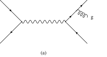
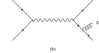
Figure 2: Real emission contribution to electron-positron annihilation.

If we define the (summed and averaged) squared matrix element as

$$\overline{\sum}|M_{3}|^{2}=\frac{1}{4}e^{4}Q_{q}^{2}g^{2}\frac{1}{s_{12}^{2}}NC_{F}\Psi\,,$$ (81)

then

$$\Psi = {\rm tr}\left[\hbox to0.0pt{\hbox{$\mskip 1.0mu/$}\hss}p_{2}\gamma^{\mu}\hbox to0.0pt{\hbox{$\mskip 1.0mu/$}\hss}p_{1}\gamma^{\nu}\right]$$ (82)

$$\times \left\{{\rm tr}\left[(\hbox to0.0pt{\hbox{$\mskip 1.0mu/$}\hss}p_{3}+m)\gamma_{\mu}(\hbox to0.0pt{\hbox{$\mskip 1.0mu/$}\hss}p_{4}+\hbox to0.0pt{\hbox{$\mskip 1.0mu/$}\hss}p_{5}-m)\gamma^{\sigma}(\hbox to0.0pt{\hbox{$\mskip 1.0mu/$}\hss}p_{4}-m)\gamma_{\sigma}(-\hbox to0.0pt{\hbox{$\mskip 1.0mu/$}\hss}p_{4}-\hbox to0.0pt{\hbox{$\mskip 1.0mu/$}\hss}p_{5}+m)\gamma_{\nu}\right]/{s_{45}^{\prime}}^{2}\right.$$

$$+2\,{\rm tr}\left[(\hbox to0.0pt{\hbox{$\mskip 1.0mu/$}\hss}p_{3}+m)\gamma^{\sigma}(\hbox to0.0pt{\hbox{$\mskip 1.0mu/$}\hss}p_{3}+\hbox to0.0pt{\hbox{$\mskip 1.0mu/$}\hss}p_{5}+m)\gamma^{\mu}(\hbox to0.0pt{\hbox{$\mskip 1.0mu/$}\hss}p_{4}-m)\gamma_{\sigma}(\hbox to0.0pt{\hbox{$\mskip 1.0mu/$}\hss}p_{4}+\hbox to0.0pt{\hbox{$\mskip 1.0mu/$}\hss}p_{5}-m)\gamma_{\nu}\right]/s_{35}^{\prime}s_{45}^{\prime}$$

$$+\left.{\rm tr}\left[(\hbox to0.0pt{\hbox{$\mskip 1.0mu/$}\hss}p_{3}+m)\gamma^{\sigma}(\hbox to0.0pt{\hbox{$\mskip 1.0mu/$}\hss}p_{3}+\hbox to0.0pt{\hbox{$\mskip 1.0mu/$}\hss}p_{5}+m)\gamma^{\mu}(-\hbox to0.0pt{\hbox{$\mskip 1.0mu/$}\hss}p_{4}+m)\gamma_{\nu}(\hbox to0.0pt{\hbox{$\mskip 1.0mu/$}\hss}p_{3}+\hbox to0.0pt{\hbox{$\mskip 1.0mu/$}\hss}p_{5}+m)\gamma_{\sigma}\right]/{s_{35}^{\prime}}^{2}\right\}\,,$$

where the strong coupling is denoted by $g$ and $C_{F}=(N^{2}-1)/2N=4/3$. To obtain the hard contribution, $\sigma_{\rm H}$, the traces may be evaluated in four space-time dimensions.

There is a soft singularity when the energy of the gluon in Fig. 2 goes to zero. The corresponding soft contribution to the cross section, $\sigma_{\rm S}$, is given by Eq. (22). In this case, the sum in (22) is taken over the final state quark legs (labeled 3 and 4) and the color connected Born cross sections are related to the leading order cross section by $d\sigma_{33}^{0}=-d\sigma_{34}^{0}=d\sigma_{44}^{0}=C_{F}d\sigma^{0}$. We find

$$d\sigma_{\rm S}=d\sigma^{0}\left[\frac{\alpha_{s}}{2\pi}\frac{\Gamma(1-\epsilon)}{\Gamma(1-2\epsilon)}\left(\frac{4\pi\mu_{r}^{2}}{s_{12}}\right)^{\epsilon}\right]C_{F}\int\left[-\frac{m^{2}}{(p_{3}\cdot p_{5})^{2}}-\frac{m^{2}}{(p_{4}\cdot p_{5})^{2}}+\frac{s-2m^{2}}{p_{3}\cdot p_{5}\,p_{4}\cdot p_{5}}\right]dS\;.$$ (83)

The poles need to be integrated over the soft phase space according to Eq. (17) to extract the singularities in dimensional regularization. Define

$$I(s_{35}^{\prime}) = \int\frac{1}{{s_{35}^{\prime}}^{2}}dS$$ (84)

$$I(s_{45}^{\prime}) = \int\frac{1}{{s_{45}^{\prime}}^{2}}dS$$ (85)

$$I(s_{35}^{\prime}s_{45}^{\prime}) = \int\frac{1}{s_{35}^{\prime}s_{45}^{\prime}}dS\,.$$ (86)

In terms of the $p_{1}p_{2}$ center-of-momentum scattering angle $\theta$, $p_{3}$ and $p_{4}$ may be written as

$$p_{3} = \frac{\sqrt{s_{12}}}{2}(1,0,\ldots,0,\beta\sin\theta,\beta\cos\theta)$$

$$p_{4} = \frac{\sqrt{s_{12}}}{2}(1,0,\ldots,0,-\beta\sin\theta,-\beta\cos\theta)\,.$$ (87)

Using these together with Eq. (12) we find

$$s_{35}^{\prime} = 2p_{3}\cdot p_{5}=\sqrt{s_{12}}E_{5}(1-\beta\sin\theta\sin\theta_{1}\cos\theta_{2}-\beta\cos\theta\cos\theta_{1})$$

$$s_{45}^{\prime} = 2p_{4}\cdot p_{5}=\sqrt{s_{12}}E_{5}(1+\beta\sin\theta\sin\theta_{1}\cos\theta_{2}+\beta\cos\theta\cos\theta_{1})\,.$$ (88)

The gluon energy integrals in Eqs. (84)–(86) may be performed trivially

$$\left(\frac{4}{s_{12}}\right)^{-\epsilon}\int_{0}^{\delta_{s}\sqrt{s_{12}}/2}dE_{5}E_{5}^{1-2\epsilon}\frac{1}{s_{12}E_{5}^{2}}=\frac{1}{s_{12}}\left(-\frac{1}{2\epsilon}\right)\delta_{s}^{-2\epsilon}\,.$$ (89)

The remaining angular integrals are well know and are tabulated in the Appendix B. The complete results are

$$I(s_{35}^{\prime})=I(s_{45}^{\prime})=\frac{1}{2m^{2}}\left(-\frac{1}{2\epsilon}+\ln\delta_{s}-\frac{1}{2\beta}\ln\frac{1+\beta}{1-\beta}\right)$$ (90)

$$I(s_{35}^{\prime}s_{45}^{\prime})=\frac{1}{s_{12}\beta}\left(-\frac{1}{2\epsilon}\ln\frac{1+\beta}{1-\beta}-\,{\rm Li_{2}}\frac{2\beta}{1+\beta}-\frac{1}{4}\ln^{2}\frac{1+\beta}{1-\beta}+\ln\delta_{s}\ln\frac{1+\beta}{1-\beta}\right)\,.$$ (91)

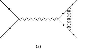
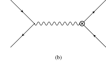
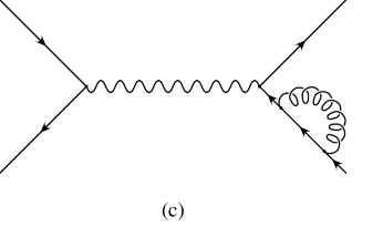
Figure 3: Loop and counterterm corrections to electron-positron annihilation via photon exchange.

We may therefore write the final expression for the soft cross section as

$$d\sigma_{\rm S}=d\sigma^{0}\left[\frac{\alpha_{s}}{2\pi}\frac{\Gamma(1-\epsilon)}{\Gamma(1-2\epsilon)}\left(\frac{4\pi\mu_{r}^{2}}{s_{12}}\right)^{\epsilon}\right]\left(\frac{A_{1}^{s}}{\epsilon}+A_{0}^{s}\right)\,,$$ (92)

where

$$A_{1}^{s} = 2C_{F}\left(1-\frac{1+\beta^{2}}{2\beta}\ln\frac{1+\beta}{1-\beta}\right)$$

$$A_{0}^{s} = 4C_{F}\left[-\ln\delta_{s}+\frac{1}{2\beta}\ln\frac{1+\beta}{1-\beta}\right.$$ (93)

$$- \left.\frac{1+\beta^{2}}{2\beta}\left(\,{\rm Li_{2}}\frac{2\beta}{1+\beta}+\frac{1}{4}\ln^{2}\frac{1+\beta}{1-\beta}-\ln\delta_{s}\ln\frac{1+\beta}{1-\beta}\right)\right]\,.$$

The virtual contribution is obtained from the one-loop diagrams shown in Fig. 3. In the on-shell renormalization scheme diagrams $(c)$ and $(d)$ cancel exactly. The vertex correction needed in Fig. 3$(a)$ is shown separately in Fig. 4. After performing the loop integrals the result for the vertex valid for $q^{2}>4m^{2}$ is

$$\Gamma_{\mu}=\left(-ieQ_{q}\right)\delta_{ij}\left(g^{2}C_{F}C_{\epsilon}\right)\overline{u}(p_{2})\left[A\frac{\left(p_{1}+p_{2}\right)_{\mu}}{2m}+B\gamma_{\mu}\right]u(p_{1})\,,$$ (94)

with

$$A = \frac{\beta^{2}-1}{\beta}\ln\frac{1-\beta}{1+\beta}$$ (95)

$$B = \frac{1}{\epsilon}\left(1+\frac{1+\beta^{2}}{\beta}\ln\frac{1+\beta}{1-\beta}\right)+3\beta\ln\frac{1+\beta}{1-\beta}$$ (96)

$$+ \frac{1+\beta^{2}}{\beta}\left(-\frac{1}{2}\ln^{2}\frac{1-\beta}{1+\beta}+2\ln\frac{1-\beta}{1+\beta}\ln\frac{2\beta}{1+\beta}+2\,{\rm Li_{2}}\frac{1-\beta}{1+\beta}+\frac{2\pi^{2}}{3}\right)\,,$$

and

$$C_{\epsilon}=\frac{\pi^{2-\epsilon}}{(2\pi)^{4-2\epsilon}}\Gamma(1+\epsilon)\left(\frac{\mu_{r}^{2}}{m^{2}}\right)^{\epsilon}\,.$$ (97)

The vertex counterterm, $Z_{1}$, implicit in Fig. 3($b$) is fixed in the on-shell renormalization scheme by the condition that the renormalized vertex through ${\cal O}(g^{2})$ evaluated at zero momentum transfer equals the leading contribution ($-ie\Lambda^{\mu}(q=0)=-ie\gamma^{\mu}$). This results in

$$Z_{1}=1-g^{2}C_{F}C_{\epsilon}\left(\frac{3}{\epsilon}+4\right)\,.$$ (98)

Figure 4: The vertex correction.

The interference of the leading order diagram with the one loop renormalized diagrams yields

$$d\sigma_{\rm V}=d\sigma^{0}\left[\frac{\alpha_{s}}{2\pi}\frac{\Gamma(1-\epsilon)}{\Gamma(1-2\epsilon)}\left(\frac{4\pi\mu_{r}^{2}}{s_{12}}\right)^{\epsilon}\right]\left(\frac{A_{1}^{v}}{\epsilon}+A_{0}^{v}\right)+d\widetilde{\sigma}^{v}\,,$$ (99)

with

$$A_{1}^{v} = -2C_{F}\left(1-\frac{1+\beta^{2}}{2\beta}\ln\frac{1+\beta}{1-\beta}\right)$$

$$A_{0}^{v} = C_{F}\left[-2\left(1-\frac{1+\beta^{2}}{2\beta}\ln\frac{1+\beta}{1-\beta}\right)\ln\left(\frac{s_{12}}{m^{2}}\right)+3\beta\ln\frac{1+\beta}{1-\beta}-4\right.$$ (100)

$$+ \left.\frac{1+\beta^{2}}{\beta}\left(-\frac{1}{2}\ln^{2}\frac{1-\beta}{1+\beta}+2\ln\frac{1-\beta}{1+\beta}\ln\frac{2\beta}{1+\beta}+2\,{\rm Li_{2}}\frac{1-\beta}{1+\beta}+\frac{2}{3}\pi^{2}\right)\right]\,,$$

and

$$d\widetilde{\sigma}^{v}=\frac{8\pi^{2}\alpha^{2}}{s_{12}}Q_{q}^{2}\left(\frac{\alpha_{s}}{2\pi}\right)\left[4NC_{F}\frac{\beta^{2}-1}{\beta}\ln\frac{1-\beta}{1+\beta}\left(\frac{m^{2}}{s_{12}}-\frac{t_{13}^{\prime}t_{14}^{\prime}}{s_{12}^{2}}\right)\right]d\Gamma_{2}\,.$$ (101)

Observe that the sum of the soft and ultra-violet renormalized virtual terms is finite, $A_{1}^{s}+A_{1}^{v}=0$, as required kln . We are therefore free to return to 4 dimensions with the finite remainders $A_{0}^{s}+A_{0}^{v}$. The final result for the ${\cal O}(\alpha_{s})$ correction consists of two contributions to the cross section: a two-body term $\sigma^{(2)}$ and a three-body term $\sigma^{(3)}$ where

$$\sigma^{(2)}=\int\left[d\sigma_{0}\left(\frac{\alpha_{s}}{2\pi}\right)\left(A_{0}^{s}+A_{0}^{v}\right)+d\widetilde{\sigma}^{v}\right]\,,$$ (102)

and

$$\sigma^{(3)}=\sigma_{H}=\frac{1}{2s_{12}}\int_{H}\overline{\sum}|M_{3}|^{2}d\Gamma_{3}\,.$$ (103)

Figure 5: The next-to-leading order contribution to the total cross section for producing a massive quark pair in electron-positron annihilation via single photon exchange. The two- and three-body contributions together with their sum are shown as a function of the soft cutoff $\delta_{s}$. The bottom enlargement shows the sum (open circles) relative to $\pm 5\%$ (dotted lines) of the analytical result (solid line) given in Eq. (104).

As a check, these results may be integrated to give a total rate and compared against the known next-to-leading order result zerwas taken from rn :

$$\sigma_{\rm tot}^{(1)} = \sigma_{0}\frac{\alpha_{s}}{4\pi}C_{F}\left[(32-8\rho^{2})\,{\rm Li_{2}}(t)+(16-4\rho^{2}){\rm F}_{3}(t)\right.$$ (104)

$$+ (2+\rho)\sqrt{1-\rho}\;{\rm F}_{4}(t)+(8-2\rho^{2})\ln(t)\ln(1+t)$$

$$+ \left.(-12+2\rho+7\rho^{2}/4)\ln(t)+(3+9\rho/2)\sqrt{1-\rho}\right]\,,$$

where $\sigma_{0}$ is the leading order cross section for producing a pair of massless quarks given by

$$\sigma_{0}=\frac{4\pi\alpha^{2}}{3s_{12}}NQ_{q}^{2}\,,$$ (105)

and we have also defined

$$t=\frac{1-\sqrt{1-\rho}}{1+\sqrt{1-\rho}}\,,$$ (106)

with $\rho=4m^{2}/s_{12}$ and

$${\rm F}_{3}(t) = \,{\rm Li_{2}}(-t)+\ln(t)\ln(1-t)$$

$${\rm F}_{4}(t) = 6\ln(t)-8\ln(1-t)-4\ln(1+t)\,.$$ (107)

The next-to-leading order corrections are shown in Fig. 5 for $\sqrt{s}=11$ GeV and $m=m_{b}=5$ GeV. The two- and three-body contributions together with their sum are shown as a function of the soft cutoff $\delta_{s}$. The bottom enlargement shows the sum (open circles) relative to $\pm 5\%$ (dotted lines) of the analytical result (solid line) given in Eq. (104). The result quickly converges to the known result.

It is satisfying that the fully inclusive rate from the slicing method agrees with that from Ref. rn . Having made this necessary check, the results may be used to histogram a wide variety observables and to study various physics issues. We refrain from any such studies here, and instead pass to our second example.

III.2 Electron-positron annihilation to massless quark pair

The process to be studied in this section is similar to that of the last section, but with one key difference: the quarks are considered massless from the beginning. Therefore, in addition to the final state soft singularities there are final state collinear singularities. The leading order cross section

$$d\sigma^{0}=\frac{1}{2s_{12}}\overline{\sum}|M_{2}|^{2}d\Gamma_{2}\,,$$ (108)

is expressed in terms of the (summed and averaged) matrix element squared

$$\overline{\sum}|M_{2}|^{2}=2Ne^{4}Q_{q}^{2}\left(\frac{t_{13}^{2}+t_{23}^{2}}{s_{12}^{2}}-\epsilon\right)\,,$$ (109)

calculated from Fig. 1, and the two body phase space

$$d\Gamma_{2}=\frac{2^{2\epsilon}}{16\pi}\left(\frac{4\pi}{s_{12}}\right)^{\epsilon}\frac{1}{\Gamma(1-\epsilon)}\int_{0}^{\pi}\sin^{1-2\epsilon}\!\theta\,d\theta\,.$$ (110)

In four space-time dimensions, integration over the phase space produces the result shown previously in Eq. (105).

For the QCD corrections we need the soft cross section (5), the hard-collinear cross section (25), the hard-non-collinear cross section (26), and the virtual contribution. The real emission diagrams are shown in Fig. 2 where the quark lines are to be interpreted as massless. The two-to-three body matrix element squared $|M_{3}|^{2}$ needed to evaluate the hard-non-collinear cross section Eq. (26) follows directly from Eq. (81) of the previous example by setting $m=0$ and evaluating the traces in four space-time dimensions. The soft cross section Eq. (5) may also be obtained from the results of the last example by setting $m=0$ in Eq. (83) giving

$$d\sigma_{\rm S}=d\sigma^{0}\left[\frac{\alpha_{s}}{2\pi}\frac{\Gamma(1-\epsilon)}{\Gamma(1-2\epsilon)}\left(\frac{4\pi\mu_{r}^{2}}{s_{12}}\right)^{\epsilon}\right]C_{F}\int\left(\frac{s}{p_{3}\cdot p_{5}\,p_{4}\cdot p_{5}}\right)dS\;.$$ (111)

The pole needs to be integrated over the soft phase space according to Eq. (17). To this end, define

$$I(s_{35}s_{45})=\int\frac{1}{s_{35}s_{45}}dS\,.$$ (112)

Using the massless ($\beta=1$) form of Eq. (88), the energy integral Eq. (89), and the angular integrals given in Appendix B, the result is

$$I(s_{35}s_{45})=\frac{1}{2s_{12}}\left(\frac{1}{\epsilon^{2}}-\frac{2}{\epsilon}\ln\delta_{s}+2\ln^{2}\delta_{s}\right)\,.$$ (113)

We may therefore write the final expression for the soft cross section as

$$d\sigma_{\rm S}=d\sigma^{0}\left[\frac{\alpha_{s}}{2\pi}\frac{\Gamma(1-\epsilon)}{\Gamma(1-2\epsilon)}\left(\frac{4\pi\mu_{r}^{2}}{s_{12}}\right)^{\epsilon}\right]\left(\frac{A_{2}^{s}}{\epsilon^{2}}+\frac{A_{1}^{s}}{\epsilon}+A_{0}^{s}\right)\,,$$ (114)

with

$$A_{2}^{s} = 2C_{F}$$

$$A_{1}^{s} = -4C_{F}\ln\delta_{s}$$

$$A_{0}^{s} = 4C_{F}\ln^{2}\delta_{s}\,.$$ (115)

The final state hard collinear cross section was derived in Sec. II.2.1. The relevant splitting is $q\rightarrow qg$. From Eq. (45) we have

$$d\sigma^{q\rightarrow qg}_{\rm HC}=d\sigma^{0}\left[\frac{\alpha_{s}}{2\pi}\frac{\Gamma(1-\epsilon)}{\Gamma(1-2\epsilon)}\left(\frac{4\pi\mu_{r}^{2}}{s_{12}}\right)^{\epsilon}\right]\left(\frac{A_{1}^{q\rightarrow qg}}{\epsilon}+A_{0}^{q\rightarrow qg}\right)\,,$$ (116)

with

$$A_{1}^{q\rightarrow qg} = C_{F}\left(3/2+2\ln\delta_{s}\right)$$

$$A_{0}^{q\rightarrow qg} = C_{F}\left[7/2-\pi^{2}/3-\ln^{2}\delta_{s}-\ln\delta_{c}\left(3/2+2\ln\delta_{s}\right)\right]\,.$$ (117)

The interference of the one-loop diagrams in Fig. 3 with the leading order diagram yields the virtual contribution. In Fig. 3, diagrams $(b)$ and $(d)$ add to zero via the Ward identity. Diagram $(c)$ vanishes for massless quarks. This leaves diagram $(a)$, comprised of the vertex shown in Fig. 4 evaluated for massless quarks. The result for the vertex is

$$\Gamma_{\mu}=\left(-ieQ_{q}\right)\delta_{ij}\overline{u}(p_{2})\gamma_{\mu}u(p_{1})\gamma(q^{2})\,,$$ (118)

with

$$\gamma(q^{2})=-\frac{\alpha_{s}}{2\pi}C_{F}\left(\frac{4\pi\mu_{r}^{2}}{-q^{2}}\right)^{\epsilon}\frac{\Gamma(1-\epsilon)}{\Gamma(1-2\epsilon)}\left(\frac{1}{\epsilon^{2}}+\frac{3}{2\epsilon}+4+\frac{\pi^{2}}{6}\right)\,.$$ (119)

We may therefore write the final expression for the virtual contribution to the cross section as

$$d\sigma_{\rm V}=d\sigma^{0}\left[\frac{\alpha_{s}}{2\pi}\frac{\Gamma(1-\epsilon)}{\Gamma(1-2\epsilon)}\left(\frac{4\pi\mu_{r}^{2}}{s_{12}}\right)^{\epsilon}\right]\left(\frac{A_{2}^{v}}{\epsilon^{2}}+\frac{A_{1}^{v}}{\epsilon}+A_{0}^{v}\right)\,,$$ (120)

with

$$A_{2}^{v} = -2C_{F}$$

$$A_{1}^{v} = -3C_{F}$$

$$A_{0}^{v} = -2C_{F}(4-\pi^{2}/3)\,.$$ (121)

Figure 6: The next-to-leading order contribution to the total cross section for producing a massless quark pair in electron-positron annihilation via single photon exchange. The two-body (negative) and three-body (positive) contributions together with their sum are shown as a function of the soft cutoff $\delta_{s}$ with the collinear cutoff $\delta_{c}=\delta_{s}/300$. The bottom enlargement shows the sum (open circles) relative to $\pm 5\%$ (dotted lines) of the analytical result (solid line) given in Eq. (124).

Figure 7: The $s_{35}-s_{45}$ plane for electron-positron annihilation to massless quarks showing the delineation into soft S and collinear C regions. The triangles marked m give vanishing contribution for $\delta_{c}\ll\delta_{s}$.

The full two-body weight is given by the sum $d\sigma_{\rm S}+d\sigma_{\rm V}+2d\sigma^{q\rightarrow qg}_{\rm HC}$. The factor of two occurs since there are two quark legs, either of which can emit a gluon. At this point we have a finite result since $A_{2}^{s}+A_{2}^{v}=0$ and $A_{1}^{s}+A_{1}^{v}+2A_{1}^{q\rightarrow qg}=0$ as required kln . The finite two-body weight is given by

$$\sigma^{(2)}=\int d\sigma_{0}\left(\frac{\alpha_{s}}{2\pi}\right)\left(A_{0}^{s}+A_{0}^{v}+2A_{0}^{q\rightarrow qg}\right)\,$$ (122)

while the three-body contribution is given by

$$\sigma^{(3)}=\sigma_{H\overline{C}}=\frac{1}{2s_{12}}\int_{H\overline{C}}\overline{\sum}|M_{3}|^{2}d\Gamma_{3}\,.$$ (123)

A necessary check may be made by integrating these results and comparing with the known analytic answer. The contributions from $\sigma^{(2)}$ (negative) and $\sigma^{(3)}$ (positive) and their sum are shown in Fig. 6 for $\sqrt{s}=500$ GeV as a function of the soft cutoff $\delta_{s}$ with the collinear cutoff $\delta_{c}=\delta_{s}/300$. The known result may be found in sterman , for example, and is given by

$$\sigma_{\rm tot}^{(1)}=\sigma_{0}\frac{\alpha_{s}}{4\pi}3C_{F}\,,$$ (124)

where $\sigma_{0}$ is given in Eq. (105). The bottom enlargement shows the sum (open circles) relative to $\pm 5\%$ (dotted lines) of the known result (solid line) given in Eq. (124). Very good agreement is found below $\delta_{s}\sim 2\times 10^{-3}$.

Before proceeding further, it is instructive to examine some issues related to the cutoff dependence of this technique. As shown in Fig. 6, the answer converges to the known result for $\delta_{s}<10^{-3}$ when $\delta_{c}=\delta_{s}/300$. We have imposed the requirement $\delta_{c}\ll\delta_{s}$ which may be understood by examining the nature of the three-body phase space for this case. Neglecting both initial and final state masses, four-momentum conservation yields $s_{12}=s_{34}+s_{35}+s_{45}$. The soft region is defined by $E_{5}<\delta_{s}\sqrt{s_{12}}/2$ which, taken with Eq. (7), can be recast as $s_{45}<\delta_{s}s_{12}-s_{35}$. This is shown as the region S in the plot of $s_{45}$ versus $s_{35}$ in Fig. 7. Two collinear regions defined by the constraints $s_{35}$ or $s_{45}<\delta_{c}s_{12}$ are shown as the regions labeled C in Fig. 7. There are two small regions labeled “m” which are properly included in the collinear regions C. However, using a fixed upper limit of $1-\delta_{s}$ in calculating the hard collinear contributions (cf. Eq. (35)) these regions are excluded. They are also not included in the hard-non-collinear three-body integrations. With some effort, it is possible to analytically evaluate the required integrals (33) over the m regions. The result (derived in Appendix C) is that occurrences of $\ln\delta_{c}\ln\delta_{s}$ in Eq. (47) are to be replaced by $\ln\delta_{c}\ln\delta_{s}-\,{\rm Li_{2}}(\delta_{c}/\delta_{s})$. From the properties of the dilogarithm function we note that the correction term vanishes like $\delta_{c}/\delta_{s}$ in the limit of small $\delta_{c}$. Accordingly, the contributions from the regions denoted by m in Fig. 7 may be made negligible by requiring $\delta_{c}\ll\delta_{s}$. Of course, as $\delta_{c}$ and $\delta_{s}$ become smaller the statistical errors on the sum of the two- and three-body weights increase. In practice, one must compromise between the errors induced by larger cutoffs and the statistical errors. For many calculations it has been found that choosing $\delta_{c}$ to be 50 - 100 times smaller than $\delta_{s}$ is sufficient for answers accurate to a few percent. Acceptable ranges for $\delta_{s}$ must be determined on a case by case basis, as illustrated by the examples shown here. Furthermore, the sign of the deviations as $\delta_{s}$ grows differs from process to process.

III.3 Electron-positron annihilation to photons

In this section we consider an example fragmentation process, inclusive photon production in hadronic final states of electron-positron annihilation, calculated to leading order in the electromagnetic coupling $\alpha$. For pedagogical purposes only the radiation of photons from the final state quark or antiquark will be included, i.e., initial state radiation will be neglected. This process is different from the previous two examples in that there are final state collinear singularities only, and they are removed through the factorization procedure.

Figure 8: Leading order non-perturbative contribution to inclusive photon production via photon exchange.

The diagram for the leading order non-perturbative contribution is shown in Fig. 8. The cross section from Eq. (52) is

$$d\sigma^{e^{+}e^{-}\rightarrow\gamma X}_{0}=\sum_{q}dzD_{\gamma/q}(z)d\sigma^{e^{+}e^{-}\rightarrow q\overline{q}}_{0}\,.$$ (125)

To simplify notation it is helpful to write the Born-level total cross section for $e^{+}e^{-}\rightarrow q\overline{q}$ in terms of that for $e^{+}e^{-}\rightarrow\mu^{+}\mu^{-}$

$$\sigma^{e^{+}e^{-}\rightarrow q\overline{q}}_{0}=NQ_{q}^{2}\sigma^{e^{+}e^{-}\rightarrow\mu^{+}\mu^{-}}_{0}\,.$$ (126)

We further denote $\sigma^{e^{+}e^{-}\rightarrow\gamma X}_{0}$ by $\sigma$, and $\sigma^{e^{+}e^{-}\rightarrow\mu^{+}\mu^{-}}_{0}$ by $\sigma_{\mu\mu}$. Taking into account $D_{\gamma/q}(z)=D_{\gamma/\overline{q}}(z)$, and letting $f$ denote the quark flavor, we arrive at the result for the leading order non-perturbative contribution

$$\frac{1}{\sigma_{\mu\mu}}\frac{d\sigma}{dz}=2N\sum_{f=1}^{n_{f}}Q_{f}^{2}D_{\gamma/f}(z)\,.$$ (127)

Figure 9: Leading order perturbative contribution to inclusive photon production via photon exchange.

Additionally, there are two- and three-body pieces that make up the leading order perturbative contribution. The Feynman diagrams are shown in Fig. 9. Because there are only final state collinear singularities present, the relevant decomposition of the two-to-three contribution to the cross section is into collinear and non-collinear terms, $\sigma=\sigma_{\rm C}+\sigma_{\rm\overline{C}}$. The collinear term $\sigma_{\rm C}$ is handled as discussed in Sec. II.2.2. In this case there are no soft singularities so the soft-collinear terms $A^{sc}$ are not present. The two-body piece follows from Eq. (II.2.2)

$$\frac{1}{\sigma_{\mu\mu}}\frac{d\sigma^{(2)}}{dz}=2N\frac{\alpha}{2\pi}\sum_{f=1}^{n_{f}}Q_{q}^{4}\widetilde{D}_{\gamma/f}(z,M_{f})\,,$$ (128)

once the replacement $\alpha_{s}\rightarrow\alpha$ is made. $\widetilde{D}_{\gamma/f}(z,M_{f})$ is as given in Eq. (64) and may be expanded using $D_{\gamma/\gamma}(x)=\delta(1-x)+{\cal O}(\alpha^{2})$ and $D_{\gamma/i}(x)={\cal O}(\alpha)$ for $i=g,q$. The leading term in $\alpha$ is therefore

$$\widetilde{D}_{\gamma/q}(z,M_{f})=\int_{z}^{1}\frac{dy}{y}\delta(1-z/y)\widetilde{P}^{\rm frag}_{\gamma q}(y)=\widetilde{P}^{\rm frag}_{\gamma q}(z)\,,$$ (129)

where $\widetilde{P}^{\rm frag}$ is as given in Eq. (65) with

$$P_{\gamma q}(z,\epsilon)=\frac{1+(1-z)^{2}-\epsilon z^{2}}{z}\,.$$ (130)

The final result for the two-body piece of the leading order perturbative contribution is

$$\frac{1}{\sigma_{\mu\mu}}\frac{d\sigma^{(2)}}{dz}=2N\frac{\alpha}{2\pi}\sum_{f=1}^{n_{f}}Q_{f}^{4}\left\{\frac{1+(1-z)^{2}}{z}\ln\left[\frac{z(1-z)\delta_{c}s}{M_{f}^{2}}\right]+z\right\}\,.$$ (131)

The complementary non-collinear piece $\sigma_{\rm\overline{C}}$ follows from the matrix element represented in Fig. 9

$$\sigma^{(3)}=\frac{1}{2s}\int_{\rm\overline{C}}\overline{\sum}|M_{3}|^{2}d\Gamma_{3}=\frac{4e^{6}}{3s^{2}}N\sum_{f=1}^{n_{f}}Q_{f}^{4}\int_{\rm\overline{C}}d\Gamma_{3}\left(\frac{2s_{34}s}{s_{35}s_{45}}+\frac{s_{35}}{s_{45}}+\frac{s_{45}}{s_{35}}\right)\,.$$ (132)

We could now study the cutoff dependence numerically as in the previous examples. However, the integration over phase space may be performed analytically and rather straightforwardly so we take this route to demonstrating the $\delta_{c}$ independence of the full result. To this end, consider, in the virtual photon rest frame, the three-body phase space

$$d\Gamma_{3}=\frac{1}{8}\frac{1}{(2\pi)^{5}}\frac{1}{E_{3}}\frac{d^{3}p_{4}}{E_{4}}\frac{d^{3}p_{5}}{E_{5}}\delta(\sqrt{s}-E_{3}-E_{4}-E_{5})\,.$$ (133)

Let $q^{\mu}$ denote the virtual photon four-momentum. Taking $\vec{p}_{5}$ along the $z$ axis and defining $x_{4}=2E_{4}/\sqrt{s}$, $z=2E_{5}/\sqrt{s}$ we may write the four-momenta as

$$q = \sqrt{s}(1,0,0,0)$$ (134)

$$p_{5} = z\frac{\sqrt{s}}{2}(1,0,0,1)$$ (135)

$$p_{4} = x_{4}\frac{\sqrt{s}}{2}(1,\sin\theta,0,\cos\theta)\,.$$ (136)

Momentum conservation $\vec{q}=\vec{p}_{3}+\vec{p}_{4}+\vec{p}_{5}$ gives

$$p_{3}=(E_{3},-x_{4}\frac{\sqrt{s}}{2}\sin\theta,0,-x_{4}\frac{\sqrt{s}}{2}\cos\theta-z\frac{\sqrt{s}}{2})\,.$$ (137)

The mass-shell condition $p_{3}^{2}=0$ can be used to fix $E_{3}$ as

$$E_{3}=\frac{\sqrt{s}}{2}\sqrt{x_{4}^{2}+z^{2}+2x_{4}z\cos\theta}\,.$$ (138)

Writing $d^{3}p_{4}=2\pi\,d\!\cos\theta E_{4}^{2}dE_{4}$ and $d^{3}p_{5}=4\pi E_{5}^{2}dE_{5}$ the phase space delta function may be used to perform the $\cos\theta$ integral. The invariants $s_{34}$, $s_{35}$, and $s_{45}$ may then be written in terms of $x_{4}$ and $z$

$$s_{35} = s(1-x_{4})$$

$$s_{45} = s(z+x_{4}-1)$$

$$s_{34} = s(1-z)\,.$$ (139)

The three-body piece is now

$$\frac{1}{\sigma_{\mu\mu}}\frac{d\sigma^{(3)}}{dz}=N\frac{\alpha}{2\pi}\sum_{f=1}^{n_{f}}Q_{f}^{4}\int_{\rm\overline{C}}dx_{4}\left[\frac{2(1-z)}{(1-x_{4})(z+x_{4}-1)}+\frac{1-x_{4}}{z+x_{4}-1}+\frac{z+x_{4}-1}{1-x_{4}}\right]\,.$$ (140)

This is to be integrated over the non-collinear ${\rm\overline{C}}$ region defined by $s_{45}>\delta_{c}s$ and $s_{35}>\delta_{c}s$ which is equivalent to $1-z+\delta_{c}\leq x_{4}\leq 1-\delta_{c}$. The integral may easily be performed. Dropping terms of ${\cal O}(\delta_{c})$, the final result for the three-body piece of the leading order perturbative contribution is

$$\frac{1}{\sigma_{\mu\mu}}\frac{d\sigma^{(3)}}{dz}=2N\frac{\alpha}{2\pi}\sum_{f=1}^{n_{f}}Q_{f}^{4}\left[\frac{1+(1-z)^{2}}{z}\ln\left(\frac{z}{\delta_{c}}\right)-z\right]\,.$$ (141)

Adding the non-perturbative (127), perturbative two-body (131), and perturbative three-body (141) contributions we obtain the well known result photon1 ; photon2

$$\frac{1}{\sigma_{\mu\mu}}\frac{d\sigma}{dz}=2N\sum_{f=1}^{n_{f}}Q_{f}^{2}\left\{D_{\gamma/f}(z)+\frac{\alpha}{2\pi}Q_{f}^{2}\frac{1+(1-z)^{2}}{z}\ln\left[\frac{z^{2}(1-z)s}{M_{f}^{2}}\right]\right\}\,,$$ (142)

which is independent of $\delta_{c}$.

III.4 Drell-Yan

Our next example is that of the QCD corrections to lepton pair production in hadron-hadron collisions which illustrates the method for handling initial state collinear singularities developed in Sec. II.2.3.

The leading order contribution mediated by a virtual photon is shown in Fig. 10. The leading order partonic cross section

$$d\hat{\sigma}^{0}=\frac{1}{2s_{12}}\overline{\sum}|M_{2}|^{2}d\Gamma_{2}\,,$$ (143)

is expressed in terms of the (summed and averaged) matrix element squared calculated in $n=4-2\epsilon$ dimensions

$$\overline{\sum}|M_{2}|^{2}=e^{4}Q_{f}^{2}\frac{2}{N}\left(\frac{t_{13}^{2}+t_{23}^{2}}{s^{2}}-\epsilon\right)\,,$$ (144)

and the two-body phase space

$$d\Gamma_{2}=\frac{2^{2\epsilon}}{16\pi}\left(\frac{4\pi}{s_{12}}\right)^{\epsilon}\frac{1}{\Gamma(1-\epsilon)}\int_{0}^{\pi}\sin^{1-2\epsilon}\!\theta\,d\theta\,.$$ (145)

Figure 10: Leading order contribution to Drell-Yan production of a lepton pair via photon exchange.

For the QCD corrections there are five pieces to consider: the finite hard-non-collinear partonic cross section Eq. (26), the mass factorized hard-collinear cross section Eq. (74), which consists of two pieces, the soft part of the initial state factorization counterterms and the mass factorization residuals (the $\widetilde{G}$ functions), the soft cross section Eq. (22), and the virtual corrections.

Shown in Fig. 11 are the real emission diagrams that give $|M_{3}|^{2}$. Defining the (summed and averaged) matrix element squared as

$$\overline{\sum}|M_{3}|^{2}=\frac{1}{4}e^{4}Q_{f}^{2}g^{2}\frac{1}{s_{34}^{2}}\frac{C_{F}}{N}\Psi\,.$$ (146)

we find

$$\Psi = {\rm tr}\left[\hbox to0.0pt{\hbox{$\mskip 1.0mu/$}\hss}p_{3}\gamma^{\mu}\hbox to0.0pt{\hbox{$\mskip 1.0mu/$}\hss}p_{4}\gamma^{\nu}\right]$$ (147)

$$\times \left\{-{\rm tr}\left[\hbox to0.0pt{\hbox{$\mskip 1.0mu/$}\hss}p_{2}\gamma_{\mu}(\hbox to0.0pt{\hbox{$\mskip 1.0mu/$}\hss}p_{1}-\hbox to0.0pt{\hbox{$\mskip 1.0mu/$}\hss}p_{5})\gamma^{\sigma}\hbox to0.0pt{\hbox{$\mskip 1.0mu/$}\hss}p_{1}\gamma_{\sigma}(\hbox to0.0pt{\hbox{$\mskip 1.0mu/$}\hss}p_{1}-\hbox to0.0pt{\hbox{$\mskip 1.0mu/$}\hss}p_{5})\gamma_{\nu}\right]/t_{15}^{2}\right.$$

$$+2\,{\rm tr}\left[\hbox to0.0pt{\hbox{$\mskip 1.0mu/$}\hss}p_{2}\gamma^{\sigma}(\hbox to0.0pt{\hbox{$\mskip 1.0mu/$}\hss}p_{2}-\hbox to0.0pt{\hbox{$\mskip 1.0mu/$}\hss}p_{5})\gamma^{\mu}\hbox to0.0pt{\hbox{$\mskip 1.0mu/$}\hss}p_{1}\gamma_{\sigma}(\hbox to0.0pt{\hbox{$\mskip 1.0mu/$}\hss}p_{1}-\hbox to0.0pt{\hbox{$\mskip 1.0mu/$}\hss}p_{5})\gamma_{\nu}\right]/t_{15}t_{25}$$

$$-\left.{\rm tr}\left[\hbox to0.0pt{\hbox{$\mskip 1.0mu/$}\hss}p_{2}\gamma^{\sigma}(\hbox to0.0pt{\hbox{$\mskip 1.0mu/$}\hss}p_{2}-\hbox to0.0pt{\hbox{$\mskip 1.0mu/$}\hss}p_{5})\gamma^{\mu}\hbox to0.0pt{\hbox{$\mskip 1.0mu/$}\hss}p_{1}\gamma_{\nu}(\hbox to0.0pt{\hbox{$\mskip 1.0mu/$}\hss}p_{2}-\hbox to0.0pt{\hbox{$\mskip 1.0mu/$}\hss}p_{5})\gamma_{\sigma}\right]/t_{25}^{2}\right\}\,.$$

The hard-non-collinear partonic cross section is obtained by evaluating the traces in four space-time dimensions.

There is a soft singularity when the gluon’s energy goes to zero in the real emission diagrams. This contributes to the soft cross section presented in Eq. (22). The sum runs over the initial state quark lines (labeled by 1 and 2). The color connected Born cross section $d\sigma_{12}^{0}=-C_{F}d\sigma^{0}$. We find

$$d\sigma_{\rm S}=d\hat{\sigma}^{0}\left[\frac{\alpha_{s}}{2\pi}\frac{\Gamma(1-\epsilon)}{\Gamma(1-2\epsilon)}\left(\frac{4\pi\mu_{r}^{2}}{s_{12}}\right)^{\epsilon}\right]C_{F}\int\left(\frac{s}{p_{1}\cdot p_{5}\,p_{2}\cdot p_{5}}\right)dS\;.$$ (148)

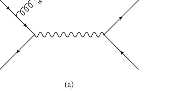
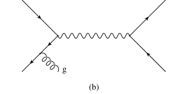
Figure 11: Real emission contribution to Drell-Yan production of a lepton pair via photon exchange.

The integration of the pole over the soft phase space measure (17) is written in terms of

$$I(t_{15}t_{25})=\int\frac{1}{t_{15}t_{25}}dS\,.$$ (149)

In the $p_{1}p_{2}$ center-of-momentum system we take

$$p_{1} = \frac{\sqrt{s_{12}}}{2}(1,0,\ldots,0,1)$$

$$p_{2} = \frac{\sqrt{s_{12}}}{2}(1,0,\ldots,0,-1)\,.$$ (150)

Using these together with Eq. (12) we find

$$t_{15} = -2p_{1}\cdot p_{5}=-\sqrt{s_{12}}E_{5}(1-\cos\theta_{1})$$

$$t_{25} = -2p_{2}\cdot p_{5}=-\sqrt{s_{12}}E_{5}(1+\cos\theta_{1})\,.$$ (151)

Using the energy integral Eq. (89) and the angular integrals given in Appendix B, we find

$$I(t_{15}t_{25})=\frac{1}{2s_{12}}\left(\frac{1}{\epsilon^{2}}-\frac{2}{\epsilon}\ln\delta_{s}+2\ln^{2}\delta_{s}\right)\,.$$ (152)

We may therefore write the final expression for the soft cross section as

$$d\sigma_{\rm S}=d\hat{\sigma}^{0}\left[\frac{\alpha_{s}}{2\pi}\frac{\Gamma(1-\epsilon)}{\Gamma(1-2\epsilon)}\left(\frac{4\pi\mu_{r}^{2}}{s_{12}}\right)^{\epsilon}\right]\left(\frac{A_{2}^{s}}{\epsilon^{2}}+\frac{A_{1}^{s}}{\epsilon}+A_{0}^{s}\right)\,,$$ (153)

with

$$A_{2}^{s} = 2C_{F}$$

$$A_{1}^{s} = -4C_{F}\ln\delta_{s}$$

$$A_{0}^{s} = 4C_{F}\ln^{2}\delta_{s}\,.$$ (154)

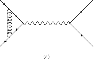
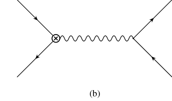
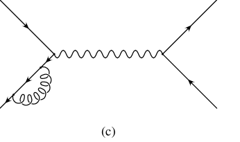
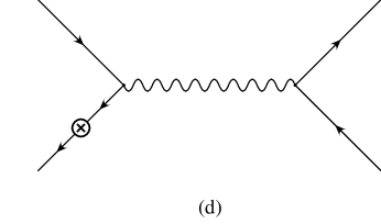
Figure 12: Loop and counterterm corrections to Drell-Yan production of a lepton pair via photon exchange.

Because the quarks are massless, there is a collinear singularity when the gluon becomes collinear to either of the initial state quark lines. This singularity is removed through the factorization program described in Sec. II.2.3. The soft-collinear pieces of the initial state factorization counterterms are given in Eq. (74) as

$$d\sigma^{\rm coll}=d\sigma^{0}\left[\frac{\alpha_{s}}{2\pi}\frac{\Gamma(1-\epsilon)}{\Gamma(1-2\epsilon)}\left(\frac{4\pi\mu_{r}^{2}}{s_{12}}\right)^{\epsilon}\right]\left(\frac{A_{1}^{\rm sc}}{\epsilon}+A_{0}^{\rm sc}\right)\,,$$ (155)

with

$$A_{1}^{\rm sc} = C_{F}\left(2\ln\delta_{s}+3/2\right)$$

$$A_{0}^{\rm sc} = C_{F}\left(2\ln\delta_{s}+3/2\right)\ln\frac{s_{12}}{\mu^{2}_{f}}\,.$$ (156)

The one-loop virtual diagrams are shown in Fig. 12. As in the case for electron-positron annihilation to a massless quark pair, diagrams $(b)$ and $(d)$ add to zero via the Ward identity, and diagram $(c)$ vanishes for massless quarks. This leaves diagram $(a)$ for which the vertex shown in Fig. 4 is needed, for massless quarks. The result is given in Eq. (118). The final expression for the virtual cross section is

$$d\sigma_{\rm V}=d\sigma^{0}\left[\frac{\alpha_{s}}{2\pi}\frac{\Gamma(1-\epsilon)}{\Gamma(1-2\epsilon)}\left(\frac{4\pi\mu_{r}^{2}}{s_{12}}\right)^{\epsilon}\right]\left(\frac{A_{2}^{v}}{\epsilon^{2}}+\frac{A_{1}^{v}}{\epsilon}+A_{0}^{v}\right)\,,$$ (157)

with

$$A_{2}^{v} = -2C_{F}$$

$$A_{1}^{v} = -3C_{F}$$

$$A_{0}^{v} = -2C_{F}(4-\pi^{2}/3)\,.$$ (158)

At this point we pause to note that the two-body weight is finite: $A_{2}^{s}+A_{2}^{v}=0$ and $A_{1}^{s}+A_{1}^{v}+2A_{1}^{\rm sc}=0$. The factor of two occurs since there are two quark legs, either of which can emit a gluon.

In addition to the $q\overline{q}$ initiated processes, there are also $qg$ initiated processes at this order of perturbation theory, as shown in Fig. 13. The singularities are initial state collinear only in origin and arise from the $P_{qg}$ splitting in diagram $(b)$. They are removed by factorization. As the $P_{qg}(z)$ kernel is finite for $z=1$ there are no soft singularities. This implies the $A^{\rm sc}$ terms in Eq. (74) are not present; only the finite $\widetilde{G}$ terms remain.

The final finite two-body cross section is given by the sum of the residual $\widetilde{G}$ terms from both the $q\overline{q}$ and $qg$ initiated processes and the finite two body weights from the $q\overline{q}$ process, $A_{0}^{s}+A_{0}^{v}+2A_{0}^{\rm sc}$. The result, summed over all parton flavors, is

$$\sigma^{(2)} = \left(\frac{\alpha_{s}}{2\pi}\right)\sum_{f}\int dx_{A}dx_{B}d\hat{\sigma}_{0}\left[G_{f/A}(x_{A},\mu_{f})G_{\overline{f}/B}(x_{B},\mu_{f})\left(A_{0}^{s}+A_{0}^{v}+2A_{0}^{\rm sc}\right)\right.$$ (159)

$$+ \left.G_{f/A}(x_{A},\mu_{f})\widetilde{G}_{\overline{f}/B}(x_{B},\mu_{f})+\widetilde{G}_{f/A}(x_{A},\mu_{f})G_{\overline{f}/B}(x_{B},\mu_{f})+(x_{A}\leftrightarrow x_{B})\right]\,.$$

The $\widetilde{G}$ functions are given in Eq. (75). The three-body contribution is given by

$$\sigma^{(3)}=\sum_{i,j=q,g}\int dx_{A}dx_{B}G_{i/A}(x_{A},\mu_{f})G_{j/B}(x_{B},\mu_{f})d\hat{\sigma}_{ij}\,,$$ (160)

with the hard-non-collinear partonic cross section given by

$$d\hat{\sigma}_{ij}=\frac{1}{2s_{12}}\int_{H\overline{C}}\overline{\sum}|M_{3}^{(ij)}|^{2}d\Gamma_{3}\,.$$ (161)

Physical predictions follow from the sum $\sigma^{(2)}+\sigma^{(3)}$ which is cutoff independent for sufficiently small cutoffs. The results may be integrated to obtain the total rate for $Q^{2}>Q^{2}_{\rm min}$ and checked against the known ${\cal O}(\alpha_{s})$ corrections

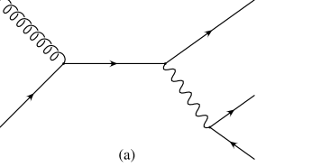
Figure 13: Quark-gluon initiated contribution to Drell-Yan production of a lepton pair.

$$\sigma=\int^{S}_{Q^{2}_{\rm min}}dQ^{2}\int^{1}_{Q^{2}/S}dx_{A}\int^{1}_{Q^{2}/Sx_{A}}dx_{B}\Biggl{\{}\sum_{ij=q,\bar{q}}G_{i/A}(x_{A},\mu_{f})G_{j/B}(x_{B},\mu_{f}){d\hat{\sigma}_{qq}\over dQ^{2}}$$ (162)

$$\quad+\sum_{i=q,\bar{q}}\Bigl{[}G_{i/A}(x_{A},\mu_{f})G_{g/B}(x_{B},\mu_{f})+G_{g/A}(x_{A},\mu_{f})G_{i/B}(x_{B},\mu_{f})\Bigr{]}{d\hat{\sigma}_{qg}\over dQ^{2}}\Biggr{\}}\,,$$

where $Q^{2}$ is the square of the lepton pair invariant mass and $S$ is the hadron-hadron center of mass energy squared which is related to $s_{12}$, the parton-parton center of mass energy squared, via $s_{12}=x_{A}x_{B}S$. Defining $z=Q^{2}/s_{12}$, the ${\cal O}(\alpha_{s})$ hard scattering partonic subprocess cross sections are given by aem

Figure 14: The next-to-leading order quark-quark contribution to the Drell-Yan cross section. The two-body (negative) and three-body (positive) contributions together with their sum are shown as a function of the soft cutoff $\delta_{s}$ with the collinear cutoff $\delta_{c}=\delta_{s}/50$. The bottom enlargement shows the sum (open circles) relative to $\pm 5\%$ (dotted lines) of the analytic result (solid line) given in Eq. (163).

$${d\hat{\sigma}_{qq}\over dQ^{2}} = \sigma_{0}{\alpha_{s}\over 2\pi}C_{F}\Biggl{\{}4(1+z^{2})\Biggl{[}{\ln(1-z)\over 1-z}\Biggr{]}_{+}-2{(1+z^{2})\over 1-z}\ln z$$ (163)

$$\quad\quad\quad\quad+\Bigl{(}{2\pi^{2}\over 3}-8\Bigr{)}\delta(1-z)+{3\over 2}P^{+}_{qq}(z)\ln{Q^{2}\over\mu_{f}^{2}}\Biggr{\}}\,,$$

and

$${d\hat{\sigma}_{qg}\over dQ^{2}} = \sigma_{0}{\alpha_{s}\over 2\pi}\frac{1}{2}\Biggl{\{}\frac{3}{2}+z-\frac{3}{2}z^{2}+2P^{+}_{qg}(z)\Biggl{[}\ln\frac{(1-z)^{2}}{z}-1+\ln{Q^{2}\over\mu_{f}^{2}}\Biggr{]}\Biggr{\}}\,,$$ (164)

where $\sigma_{0}$

$$\sigma_{0}=\frac{4\pi\alpha^{2}Q_{q}^{2}}{3Ns_{12}Q^{2}}\,.$$ (165)

$P^{+}_{qq}(z)$ and $P^{+}_{qg}(z)$ are the splitting kernels given in Eqs. (55) and (58).

We show numerical results on the cutoff (in)dependence for proton-proton collisions at $\sqrt{S}=28.28$ GeV with $Q_{min}=10$ GeV. Hard scales are set to the lepton pair mass $\mu_{f}=\mu_{r}=Q$ and the number of flavors taken to be $n_{f}=3$.

Shown in Fig. 14 is the next-to-leading order quark-quark contribution to the Drell-Yan cross section. The two- and three-body contributions to the cross section (negative and positive, respectively), and their sum are shown as a function of the soft cutoff $\delta_{s}$. The collinear cutoff $\delta_{c}=\delta_{s}/50$. The bottom portion of the figure shows the sum (open circles) relative to $\pm 5\%$ (dotted lines) of the analytic result (solid line) given in Eq. (163).

Figure 15: The next-to-leading order quark-gluon contribution to the Drell-Yan cross section. The two-body (negative) and three-body (positive) contributions together with their sum are shown as a function of the collinear cutoff $\delta_{c}$. The bottom enlargement shows the sum (open circles) relative to $\pm 5\%$ (dotted lines) of the analytic result (solid line) given in Eq. (164).

Finally, we show the next-to-leading order quark-gluon contribution to the Drell-Yan cross section in Fig. 15. The two- and three-body contributions and their sum are shown as a function of the collinear cutoff $\delta_{c}$. The bottom enlargement shows the sum (open circles) relative to $\pm 5\%$ (dotted lines) of the analytic result (solid line) given in Eq. (164).

In both cases, nice agreement is seen with the known analytic result, providing a cross check on the use of the two cutoff phase space slicing method.

III.5 Single Particle Inclusive Cross Section

Our final example is that of the single particle inclusive cross section in hadron-hadron collisions. The input needed for this calculation includes the squared matrix elements for the $2\rightarrow 3$ subprocesses es and the results for the ${\cal O}(\alpha_{s}^{3})$ one-loop contributions to the $2\rightarrow 2$ subprocesses ks ; es . For the purpose of this example, the notation of ks will be used, since much of the input needed can be found in the appendices of that paper. The partons are labelled as $A+B\rightarrow 1+2$  and $A+B\rightarrow 1+2+3$  for the $2\rightarrow 2$  and $2\rightarrow 3$ subprocesses, respectively. A flavor label $a_{A}$ is used to denote the flavor of parton $A$, and similarly for the other partons.

The lowest-order contribution to the inclusive cross section for producing a hadron $h$ in a collision of hadrons of types $A$ and $B$ can be written as

$$d\sigma^{B} = \frac{1}{2x_{A}x_{B}s}\sum_{a_{A},a_{B},a_{1},a_{2}}G_{a_{A}/A}(x_{A})G_{a_{B}/B}(x_{B})D_{h/a_{1}}(z_{1})dx_{A}\,dx_{B}\,dz_{1}\,$$ (166)

$$\times \frac{(4\pi\alpha_{s})^{2}}{w(a_{A})w(a_{B})}\psi^{(4)}(\vec{a},\vec{p})d\Gamma_{2}$$

where $\vec{a}=\{a_{A},a_{B},a_{1},a_{2}\}$ and $\vec{p}=\{p_{A}^{\mu},p_{B}^{\mu},p_{1}^{\mu},p_{2}^{\mu}\}$ denote the sets of flavor indices and parton four-vectors, respectively. The factors appearing in the spin/color averaging are given by

$$w(a)=\left\{\begin{array}[]{ll}2(1-\epsilon)V&\mbox{a=gluon}\\ 2N&\mbox{a=quark or antiquark}\end{array}\right.$$

with $N=3$ and $V=N^{2}-1.$ The factor $d\Gamma_{2}$ is the differential two-body phase space element from Eq. (11). Eq. (166) gives the contribution where parton 1 fragments into the hadron $h$. Care must be taken to explicitly include in the sum over $\vec{a}$ those terms corresponding to the case where parton 2 fragments into $h$. For compactness, these terms will not be explicitly written. The squared matrix elements for the various subprocesses, denoted by $\psi^{(4)}(\vec{a},\vec{p})$, may be found in Ref. ks .

Next, consider the one-loop virtual corrections to the $2\rightarrow 2$ subprocesses. These take the form

$$d\sigma^{v} = \frac{1}{2x_{A}x_{B}s}\sum_{a_{A},a_{B},a_{1},a_{2}}G_{a_{A}/A}(x_{A})G_{a_{B}/B}(x_{B})D_{h/a_{1}}(z_{1})dx_{A}\,dx_{B}\,dz_{1}$$ (167)

$$\times \frac{(4\pi\alpha_{s})^{2}}{w(a_{A})w(a_{B})}\left[\frac{\alpha_{s}}{2\pi}\left(\frac{4\pi\mu^{2}_{R}}{2p_{A}\cdot p_{B}}\right)^{\epsilon}\frac{\Gamma(1-\epsilon)}{\Gamma(1-2\epsilon)}\right]\psi^{(6)}(\vec{a},\vec{p})d\Gamma_{2}$$

where

$$\psi^{(6)}(\vec{a},\vec{p}) = \psi^{(4)}(\vec{a},\vec{p})\left[-\frac{1}{\epsilon^{2}}\sum_{n}C(a_{n})-\frac{1}{\epsilon}\sum_{n}\gamma(a_{n})\right]$$ (168)

$$+ \frac{1}{2\epsilon}\sum_{m,n\atop m\neq n}\ln\left(\frac{p_{m}\cdot p_{n}}{p_{A}\cdot p_{B}}\right)\psi^{(4,c)}_{m,n}(\vec{a},\vec{p})$$

$$- \frac{\pi^{2}}{6}\sum_{n}\psi^{(4)}(\vec{a},\vec{p})+\psi^{(6)}_{NS}(\vec{a},\vec{p})+{\cal O}(\epsilon).$$

This expression for $\psi^{(6)}$ differs slightly from Eq. (35) in Ref. ks because we have chosen to extract a different $\epsilon$ dependent overall factor: a factor of $\Gamma(1+\epsilon)\Gamma(1-\epsilon)\approx 1+\epsilon^{2}\frac{\pi^{2}}{6}$ has been absorbed into the above expression for $\psi^{(6)}$. Furthermore, the arbitrary scale $Q_{ES}^{2}$ used in Ref. ks has, in order to match the conventions used elsewhere in the present work, been chosen to be $2p_{A}\cdot p_{B}$. The expressions for the functions $\psi^{(4,c)}_{m,n}$  and $\psi^{(6)}_{NS}$ may be found in Appendix B of Ref. ks . The quantities $C(a_{n})$  and $\gamma(a_{n})$ are given by

$$C(a)=\left\{\begin{array}[]{ll}N=3&\mbox{a=gluon}\\ C_{F}=\frac{4}{3}&\mbox{a=quark or antiquark}\end{array}\right.$$

and

$$\gamma(a)=\left\{\begin{array}[]{ll}(11N-2n_{f})/6&\mbox{a=gluon}\\ 3C_{F}/2&\mbox{a=quark or antiquark}\end{array}\right.$$

It will be convenient for subsequent expressions to adopt the following notation:

$${\cal F}=\left(\frac{4\pi\mu^{2}_{R}}{2p_{A}\cdot p_{B}}\right)^{\epsilon}\frac{\Gamma(1-\epsilon)}{\Gamma(1-2\epsilon)}.$$ (169)

The one loop virtual contributions can now be written as

$$d\sigma^{v} = \frac{1}{2x_{A}x_{B}s}\sum_{a_{A},a_{B},a_{1},a_{2}}G_{a_{A}/A}(x_{A})G_{a_{B}/B}(x_{B})D_{h/a_{1}}(z_{1})dx_{A}\,dx_{B}\,dz_{1}$$ (170)

$$\times \frac{(4\pi\alpha_{s})^{2}}{w(a_{A})w(a_{B})}{\cal F}\frac{\alpha_{s}}{2\pi}\left(\frac{A_{2}^{v}}{\epsilon^{2}}+\frac{A_{1}^{v}}{\epsilon}+A_{0}^{v}\right)d\Gamma_{2}$$

where

$$A_{2}^{v} = -\sum_{n}C(a_{n})\psi^{(4)}(\vec{a},\vec{p})$$ (171)

$$A_{1}^{v} = -\sum_{n}\gamma(a_{n})\psi^{(4)}(\vec{a},\vec{p})+\frac{1}{2}\sum_{m,n\atop m\neq n}\ln\left(\frac{p_{m}\cdot p_{n}}{p_{A}\cdot p_{B}}\right)\psi^{(4,c)}_{m,n}(\vec{a},\vec{p})$$ (172)

$$A_{0}^{v} = -\frac{\pi^{2}}{6}\sum_{n}C(a_{n})\psi^{(4)}(\vec{a},\vec{p})+\psi^{(6)}_{NS}(\vec{a},\vec{p}).$$ (173)

Next, the contributions from the $2\rightarrow 3$ subprocesses in the limit where one of the final state gluons becomes soft are needed. The contributions of the $2\rightarrow 3$ subprocesses may be written as

$$d\sigma^{2\rightarrow 3} = \frac{1}{2x_{A}x_{B}s}\frac{(4\pi\alpha_{s})^{3}}{w(a_{A})w(a_{B})}{\cal F}\sum_{a_{A},a_{B},a_{1},a_{2},a_{3}}G_{a_{A}/A}(x_{A})G_{a/B/B}(x_{B})D_{h/a_{1}}(z_{1})dx_{A}\,dx_{B}\,dz_{1}\,$$ (174)

$$\times \Psi(a_{A},a_{B},a_{1},a_{2},a_{3},p_{A}^{\mu},p_{B}^{\mu},p_{1}^{\mu},p_{2}^{\mu},p_{3}^{\mu})d\Gamma_{3}.$$

The expressions for the $2\rightarrow 3$ squared matrix elements appearing in Eq. (174) may be found in Ref. es . As noted earlier for the two-body contributions, one must include in the sum all possible parton to hadron fragmentations.

Consider the case where the soft gluon is parton 3. In this limit, the function $\Psi$ may be expanded as:

$$\Psi(a_{A},a_{B},a_{1},a_{2},a_{3},p_{A}^{\mu},p_{B}^{\mu},p_{1}^{\mu},p_{2}^{\mu},p_{3}^{\mu})\sim\sum_{m,n\atop m<n}\delta_{a_{3},g}\frac{p_{m}\cdot p_{n}}{p_{m}\cdot p_{3}p_{n}\cdot p_{3}}\psi^{(4,c)}_{m,n}(a_{A},a_{B},a_{1},a_{2},p_{A}^{\mu},p_{B}^{\mu},p_{1}^{\mu},p_{2}^{\mu}).$$ (175)

Next, one must integrate over the soft region of phase space defined by $E_{3}<\delta_{s}\sqrt{2p_{A}\cdot p_{B}}/2$. This is easily done using the integrals given in the appendix. The resulting soft contribution may be written as

$$d\sigma^{s} = \frac{1}{2x_{A}x_{B}s}\sum_{a_{A},a_{B},a_{1},a_{2}}G_{a_{A}/A}(x_{A})G_{a_{B}/B}(x_{B})D_{h/a_{1}}(z_{1})dx_{A}\,dx_{B}\,dz_{1}$$ (176)

$$\times \frac{(4\pi\alpha_{s})^{2}}{w(a_{A})w(a_{B})}{\cal F}\frac{\alpha_{s}}{2\pi}\left(\frac{A_{2}^{s}}{\epsilon^{2}}+\frac{A_{1}^{s}}{\epsilon}+A_{0}^{s}\right)d\Gamma_{2}$$

where

$$A_{2}^{s} = \sum_{n}C(a_{n})\psi^{(4)}(\vec{a},\vec{p})$$ (177)

$$A_{1}^{s} = -2\ln\delta_{s}\sum_{n}C(a_{n})\psi^{(4)}(\vec{a},\vec{p})-\frac{1}{2}\sum_{m,n\atop m\neq n}\ln\left(\frac{p_{m}\cdot p_{n}}{p_{A}\cdot p_{B}}\right)\psi^{(4,c)}_{m,n}(\vec{a},\vec{p})$$ (178)

$$A_{0}^{s} = 2\ln^{2}\delta_{s}\sum_{n}C(a_{n})\psi^{(4)}(\vec{a},\vec{p})$$ (179)

$$+ \left(\psi^{(4,c)}_{A,1}+\psi^{(4,c)}_{B,2}\right)\left[\frac{1}{2}\ln^{2}\left(\frac{p_{1}\cdot p_{3}}{p_{A}\cdot p_{B}}\right)+\,{\rm Li_{2}}\left(\frac{p_{2}\cdot p_{3}}{p_{A}\cdot p_{B}}\right)+2\ln\delta_{s}\ln\left(\frac{p_{1}\cdot p_{3}}{p_{A}\cdot p_{B}}\right)\right]$$

$$+ \left(\psi^{(4,c)}_{A,2}+\psi^{(4,c)}_{B,1}\right)\left[\frac{1}{2}\ln^{2}\left(\frac{p_{2}\cdot p_{3}}{p_{A}\cdot p_{B}}\right)+\,{\rm Li_{2}}\left(\frac{p_{1}\cdot p_{3}}{p_{A}\cdot p_{B}}\right)+2\ln\delta_{s}\ln\left(\frac{p_{2}\cdot p_{3}}{p_{A}\cdot p_{B}}\right)\right].$$

After the collinear singularities associated with the two parton distribution functions and the fragmentation function have been factorized and absorbed into the corresponding bare functions, there will be soft-collinear terms left over due to the mismatch between the integration limits of the collinear singularity terms and the factorization counterterms. In addition, there can be collinear singularities associated with the non-fragmenting parton in the final state, corresponding to gluon emission or $q\overline{q}$ production. Collecting together both types of collinear terms, the result can be written as follows:

$$d\sigma^{coll} = \frac{1}{2x_{A}x_{B}s}\sum_{a_{A},a_{B},a_{1},a_{2}}G_{a_{A}/A}(x_{A})G_{a_{B}/B}(x_{B})D_{h/a_{1}}(z_{1})dx_{A}\,dx_{B}\,dz_{1}$$ (180)

$$\times \frac{(4\pi\alpha_{s})^{2}}{w(a_{A})w(a_{B})}{\cal F}\frac{\alpha_{s}}{2\pi}\left(\frac{A_{1}^{coll}}{\epsilon}+A_{0}^{coll}\right)d\Gamma_{2}$$

where

$$A_{1}^{coll} = \sum_{n}[2\ln\delta_{s}C(a_{n})+\gamma(a_{n})]$$ (181)

$$A_{0}^{coll} = \sum_{A,B}[2\ln\delta_{s}C(a_{n})+\gamma(a_{n})]\ln\left(\frac{2p_{A}\cdot p_{B}}{\mu^{2}_{f}}\right)+[2\ln\delta_{s}C(a_{1})+\gamma(a_{1})]\ln\left(\frac{2p_{A}\cdot p_{B}}{M^{2}_{f}}\right)$$ (182)

$$+ \gamma^{\prime}(a_{2}).$$

Here $\mu_{f}\mbox{\ and \ }M_{f}$ are the initial and final state factorization scales. The function $\gamma^{\prime}(a)$ is given in terms of the hard collinear factors of Eqs. (46) – (51) as

$$\gamma^{\prime}(a)=\left\{\begin{array}[]{ll}A_{0}^{q\rightarrow qg}&\mbox{a= quark or antiquark}\\ A_{0}^{g\rightarrow gg}+A_{0}^{g\rightarrow q\bar{q}}&\mbox{a = gluon}\end{array}\right.$$ (183)

After the mass factorization has been performed, the bare parton distribution functions and fragmentation functions have been replaced by scale dependent $\overline{\mbox{MS}}$ functions. In addition, there are finite remainders involving the $\widetilde{G}\mbox{\ and \ }\widetilde{D}$ functions:

$$d\widetilde{\sigma} = \frac{1}{2x_{A}x_{B}s}\sum_{a_{A},a_{B},a_{1},a_{2}}\frac{(4\pi\alpha_{s})^{2}}{w(a_{A})w(a_{B})}\frac{\alpha_{s}}{2\pi}dx_{A}dx_{B}dz_{1}\psi^{(4)}(\vec{a},\vec{p})d\Gamma_{2}$$ (184)

$$\times \left[\widetilde{G}_{a_{A}/A}(x_{A},\mu^{2}_{f})G_{a_{B}/B}(x_{B},\mu^{2}_{f})D_{h/a_{1}}(z_{1},M^{2}_{f})\right.$$

$$+ G_{a_{A}/A}(x_{A},\mu^{2}_{f})\widetilde{G}_{a_{B}/B}(x_{B},\mu^{2}_{f})D_{h/a_{1}}(z_{1},M^{2}_{f})$$

$$+ \left.G_{a_{A}/A}(x_{A},\mu^{2}_{f})G_{a_{B}/B}(x_{B},\mu^{2}_{f})\widetilde{D}_{h/a_{1}}(z_{1},M^{2}_{f})\right].$$

At this point, all of the singular terms have been isolated as poles in $\epsilon$ or have been factorized and absorbed into the bare parton distribution and fragmentation functions. The $\epsilon$ dependent pole terms all cancel amongst each other:

$$A_{2}^{v}+A_{2}^{s}=0$$ (185)

$$A_{1}^{v}+A_{1}^{s}+A_{1}^{coll}=0.$$ (186)

The finite two-body contribution is given by

$$d\sigma^{2\rightarrow 2} = d\sigma^{B}+d\widetilde{\sigma}$$ (187)

$$+ \frac{1}{x_{A}x_{B}s}\sum_{a_{A},a_{B},a_{1},a_{2}}\frac{(4\pi\alpha_{s})^{2}}{w(a_{A})w(a_{B})}G_{a_{A}/A}(x_{A},\mu^{2}_{f})G_{a_{B}/B}(x_{B},\mu^{2}_{f})D_{h/a_{1}}(z_{1},M^{2}_{f})$$

$$\times \frac{\alpha_{s}}{2\pi}\left[A_{0}^{v}+A_{0}^{s}+A_{0}^{coll}\right]dx_{A}\,dx_{B}\,dz_{1}\,d\Gamma_{2}.$$

The three-body contribution, now evaluated in four dimensions, was given in Eq. (174) where now the soft and collinear regions of phase space are excluded.

As in the previous examples, the structure of the final result is two finite contributions, both of which depend on the soft and collinear cutoffs – one explicitly and one through the boundaries imposed on the three-body phase space. However, when both contributions are added while calculating an observable quantity, all dependence on the cutoffs cancels when sufficiantly small values of the cutoffs are used.

IV Discussion and Conclusions

A technique for performing next-to-leading-logarithm calculations using Monte Carlo techniques was described in detail. The method uses two cutoff parameters which serve to separate the regions of phase space containing the soft and collinear singularities from the non-singular regions. The main derivations for experimentally degenerate, tagged, and heavy quark final states were given, as was a discussion of initial state factorization. We provided five illustrative examples applying the method.

The first example was that of the QCD corrections to electron-positron annihilation into a massive quark pair. The quark mass serves to regulate any would-be final state collinear singularities. The final state soft singular region is delineated using one cutoff. The second example was that of QCD corrections to electron-positron annihilation into a massless quark pair. In this case final state soft and collinear singularities are encountered. Both soft and collinear cutoffs are therefore required. They should be chosen such that $\delta_{c}\ll\delta_{s}$. The third example of inclusive photon production in hadronic final states of electron-positron annihilation was presented, illustrating the use of fragmentation functions. Finally, the QCD corrections to lepton pair and single particle production in hadron-hadron collisions were given. These examples include both initial and final state soft and collinear singularities. The use of scale dependent parton distribution and fragmentation functions was explained.

The Monte Carlo results, integrated to give an inclusive cross section, were shown to be in complete agreement with those available in the literature. This is not the end of the utility of the method, but only the beginning. Given the full access to the parton four vectors and corresponding weights, we are free to combine them in any way that is consistent with an infrared-safe measurement function, which may include a jet finding algorithm and experimental cuts.

The method has been applied to a wide range of hard scattering processes and it has been found to be both simple to implement and numerically robust.

Appendix A Comparison with other methods

The essential difference between the phase space slicing and the subtraction methods may be gleaned from the following simple example ks . Consider an integral to be calculated:

$$I=\lim_{\epsilon\rightarrow 0^{+}}\left\{\int_{0}^{1}\frac{dx}{x}x^{\epsilon}F(x)-\frac{1}{\epsilon}F(0)\right\}\,,$$ (188)

where $F(x)$ is a known but complicated function related to a two-to-three body matrix element. The variable $x$ represents either the energy of an emitted gluon or the angle between two massless partons. In a traditional fully or single particle inclusive calculation the integral $I$ would be performed completely analytically.

In the subtraction method one simply adds and subtracts $F(0)$ under the integral sign.

$$I = \lim_{\epsilon\rightarrow 0^{+}}\left\{\int_{0}^{1}\frac{dx}{x}x^{\epsilon}\left[F(x)-F(0)+F(0)\right]-\frac{1}{\epsilon}F(0)\right\}$$ (189)

$$= \int_{0}^{1}\frac{dx}{x}\left[F(x)-F(0)\right]\,,$$

giving a finite and numerically calculable result. No approximations are made, however in any numerical implementation there will necessarily be a lower limit related to machine precision below which the integral must be cutoff. This is not a problem in practice.

In the phase space slicing method, the integration region is divided into two parts $0<x<\delta$ and $\delta<x<1$ with $\delta\ll 1$. A Maclaurin expansion of $F(x)$ yields

$$I = \lim_{\epsilon\rightarrow 0^{+}}\left\{\int_{0}^{\delta}\frac{dx}{x}x^{\epsilon}F(x)+\int_{\delta}^{1}\frac{dx}{x}x^{\epsilon}F(x)-\frac{1}{\epsilon}F(0)\right\}$$ (190)

$$= \int_{\delta}^{1}\frac{dx}{x}F(x)+F(0)\ln\delta+{\cal O}(\delta)\,.$$

Clearly, the parameter $\delta$ must be chosen small enough so that the term linear in $\delta$ may be neglected. At the same time it must not be so small as to spoil the numerical convergence of the first term.

Appendix B Soft Integrals

In evaluating the soft integrals we encounter angular integrals which may be written in the form

$$I^{(k,l)}_{n}=\int_{0}^{\pi}d\theta_{1}\sin^{n-3}\theta_{1}\int_{0}^{\pi}d\theta_{2}\sin^{n-4}\theta_{2}\frac{(a+b\cos\theta_{1})^{-k}}{(A+B\cos\theta_{1}+C\sin\theta_{1}\cos\theta_{2})^{l}}\,.$$ (191)

A large collection of these appear in the appendix of been . Others may be found in the appendix of hs or else computed as explained in willy . Here we collect together the results covering most of the cases encountered using the two cutoff slicing method. The first two are from hs with $A^{2}\neq B^{2}+C^{2}$

$$I^{(0,1)}_{n} = \frac{\pi}{\sqrt{B^{2}+C^{2}}}\left\{\ln\left(\frac{A+\sqrt{B^{2}+C^{2}}}{A-\sqrt{B^{2}+C^{2}}}\right)\right.$$

$$\left.-(n-4)\left[\,{\rm Li_{2}}\left(\frac{2\sqrt{B^{2}+C^{2}}}{A+\sqrt{B^{2}+C^{2}}}\right)+\frac{1}{4}\ln^{2}\left(\frac{A+\sqrt{B^{2}+C^{2}}}{A-\sqrt{B^{2}+C^{2}}}\right)\right]\right\}$$

$$I^{(0,2)}_{n}=\frac{2\pi}{A^{2}-B^{2}-C^{2}}\left[1-\frac{1}{2}(n-4)\frac{A}{\sqrt{B^{2}+C^{2}}}\ln\left(\frac{A+\sqrt{B^{2}+C^{2}}}{A-\sqrt{B^{2}+C^{2}}}\right)\right]\,,$$ (193)

where we drop $O((n-4)^{2})$ terms. The second two are from been with $b=-a$. If $A^{2}=B^{2}+C^{2}$

$$I^{(1,1)}_{n}=2\pi\frac{1}{aA}\frac{1}{n-4}\left(\frac{A+B}{2A}\right)^{n/2-3}\left[1+\frac{1}{4}(n-4)^{2}\,{\rm Li_{2}}\left(\frac{A-B}{2A}\right)\right]\,,$$ (194)

whereas if $A^{2}\neq B^{2}+C^{2}$

$$I^{(1,1)}_{n} = \frac{\pi}{a(A+B)}\left\{\frac{2}{n-4}+\ln\left[\frac{(A+B)^{2}}{A^{2}-B^{2}-C^{2}}\right]\right.$$ (195)

$$+ \left.\frac{1}{2}(n-4)\left[\ln^{2}\left(\frac{A-\sqrt{B^{2}+C^{2}}}{A+B}\right)-\frac{1}{2}\ln^{2}\left(\frac{A+\sqrt{B^{2}+C^{2}}}{A-\sqrt{B^{2}+C^{2}}}\right)\right.\right.$$

$$+ \left.\left.2\,{\rm Li_{2}}\left(-\frac{B+\sqrt{B^{2}+C^{2}}}{A-\sqrt{B^{2}+C^{2}}}\right)-2\,{\rm Li_{2}}\left(\frac{B-\sqrt{B^{2}+C^{2}}}{A+B}\right)\right]\right\},$$

again dropping $O((n-4)^{2})$ terms in the second of these. The dilogarithm function $\,{\rm Li_{2}}(x)$ is defined in dilog and numerous useful properties are summarized in dd .

Appendix C Recovering the ${\cal O}(\delta_{c}/\delta_{s})$ terms

In this appendix we integrate the $P_{qq}(z,\epsilon)$ splitting kernel over the hard-collinear portion of phase space for the case of a 45 singularity as it pertains to the discussion given at the end of Sec. III.2. Recall that this region is defined by

$${\rm hard} : \delta_{s}\frac{\sqrt{s_{12}}}{2}\leq E_{5}\leq\frac{\sqrt{s_{12}}}{2}$$

$${\rm collinear} : 0\leq s_{45}\leq\delta_{c}s_{12}\,.$$ (196)

From Eq. (29) we have $s_{34}=(p_{3}+p_{4})^{2}=2p_{3}\cdot p_{4}\simeq(2p_{3}\cdot p_{45})z$ and $s_{12}=(p_{3}+p_{45})^{2}\simeq s_{45}+2p_{3}\cdot p_{45}$ which together yield $s_{34}\simeq z(s_{12}-s_{45})$. Using $E_{5}=(s_{12}-s_{34})/2\sqrt{s_{12}}$ the hard condition becomes

$$0\leq z\leq\frac{1-\delta_{s}}{1-s_{45}/s_{12}}\,.$$ (197)

The approximation made in Sec. II.2.1 was to set $s_{45}=0$ in the denominator, in light of the collinear condition. This resulted in a decoupling of the $z$ and $s_{45}$ integration limits in Eq. (36). Relaxing the $s_{45}=0$ approximation gives rise to terms ${\cal O}(\delta_{c}/\delta_{s})$ as now described.

Keeping the $s_{45}$ dependence, the required integral is

$$I=\int_{0}^{\delta_{c}s_{12}}\frac{ds_{45}}{s_{45}}\left(\frac{s_{45}}{s_{12}}\right)^{-\epsilon}\int_{0}^{\frac{1-\delta_{s}}{1-s_{45}/s_{12}}}dz[z(1-z)]^{-\epsilon}P_{qq}(z,\epsilon)\,.$$ (198)

We may expand $P_{qq}(z,\epsilon)$ about $\epsilon=0$ and make a change of variables $u=s_{45}/s_{12}$ giving

$$I=C_{F}\int_{0}^{\delta_{c}}u^{-1-\epsilon}F(u)\,du\,,$$ (199)

with

$$F(u)=\int_{0}^{\frac{1-\delta_{s}}{1-u}}dz\left\{\frac{1+z^{2}}{1-z}-\epsilon(1-z)-\epsilon\ln\left[z(1-z)\right]\frac{1+z^{2}}{1-z}\right\}\,.$$ (200)

$F(u)$ may be evaluated with the help of

$$\int_{0}^{a}dz\,\frac{1+z^{2}}{1-z} = -a\left(1+\frac{a}{2}\right)-2\ln(1-a)$$ (201)

$$\int_{0}^{a}dz\,(1-z) = a\left(1-\frac{a}{2}\right)$$ (202)

$$\int_{0}^{a}dz\,\frac{\ln z}{1-z} = \,{\rm Li_{2}}(1-a)-\frac{\pi^{2}}{6}$$ (203)

$$\int_{0}^{a}dz\,\frac{\ln(1-z)}{1-z} = -\frac{1}{2}\ln^{2}(1-a)$$ (204)

$$\int_{0}^{a}dz\,\frac{z^{2}\ln z}{1-z} = a\left(1+\frac{a}{4}\right)-a\left(1+\frac{a}{2}\right)\ln a+\,{\rm Li_{2}}(1-a)-\frac{\pi^{2}}{6}$$ (205)

$$\int_{0}^{a}dz\,\frac{z^{2}\ln(1-z)}{1-z} = \frac{3}{2}a\left(1+\frac{a}{6}\right)+\ln(1-a)\left[\frac{3}{2}-a\left(1+\frac{a}{2}\right)-\frac{1}{2}\ln(1-a)\right]\,.$$ (206)

The resulting terms in $F(u)$ may be integrated over $u$ using

$$\int_{0}^{\delta_{c}}du\,u^{-1-\epsilon}\left(\frac{1-\delta_{s}}{1-u}\right)^{i} = \left(-\frac{1}{\epsilon}+\ln\delta_{c}\right);\quad i=0,1,2$$ (207)

$$\int_{0}^{\delta_{c}}du\,u^{-1-\epsilon}\ln\left(1-\frac{1-\delta_{s}}{1-u}\right) = \left(-\frac{1}{\epsilon}+\ln\delta_{c}\right)\ln\delta_{s}-\,{\rm Li_{2}}(\delta_{c}/\delta_{s})\,,$$ (208)

for the terms multiplied by ${\cal O}(\epsilon^{0})$ in Eq. (200) and

$$\int_{0}^{\delta_{c}}du\,u^{-1-\epsilon}\ln^{2}\left(1-\frac{1-\delta_{s}}{1-u}\right) = -\frac{1}{\epsilon}\ln^{2}\delta_{s}$$ (209)

$$\int_{0}^{\delta_{c}}du\,u^{-1-\epsilon}\left(\frac{1-\delta_{s}}{1-u}\right)^{i}\ln\left(1-\frac{1-\delta_{s}}{1-u}\right) = -\frac{1}{\epsilon}\ln\delta_{s};\quad i=1,2$$ (210)

$$\int_{0}^{\delta_{c}}du\,u^{-1-\epsilon}\left(\frac{1-\delta_{s}}{1-u}\right)^{i}\ln\left(\frac{1-\delta_{s}}{1-u}\right) = 0;\quad i=1,2$$ (211)

$$\int_{0}^{\delta_{c}}du\,u^{-1-\epsilon}\,{\rm Li_{2}}\left(1-\frac{1-\delta_{s}}{1-u}\right) = 0\,,$$ (212)

for the terms multiplied by ${\cal O}(\epsilon^{1})$ in Eq. (200). Terms containing or leading to contributions of ${\cal O}(\delta_{c})$ or ${\cal O}(\delta_{s})$ have been dropped. Taking the coefficients of $1/\epsilon$ and $\epsilon^{0}$ gives the desired result

$$A^{q\rightarrow qg}_{1} = C_{F}\left(3/2+2\ln\delta_{s}\right)$$ (213)

$$A^{q\rightarrow qg}_{0} = C_{F}\left[7/2-\pi^{2}/3-\ln^{2}\delta_{s}+2\,{\rm Li_{2}}(\delta_{c}/\delta_{s})-\ln\delta_{c}\left(3/2+2\ln\delta_{s}\right)\right]\,.$$ (214)

The second equation is identically Eq. (47) with the addition of the advertised $\,{\rm Li_{2}}(\delta_{c}/\delta_{s})$ term. A similar analysis may be performed for the $P_{gg}$ splitting case with the same result: $\ln\delta_{c}\ln\delta_{s}\rightarrow\ln\delta_{c}\ln\delta_{s}-\,{\rm Li_{2}}(\delta_{c}/\delta_{s})$.

Appendix D Improving convergence of tilde terms

We want to demonstrate how the numerical convergence of the $\widetilde{D}$ and $\widetilde{G}$ functions may be improved. To this end consider the integral

$$F_{i}=\int_{x}^{1-\delta_{s}}\frac{dy}{y}G_{j}(x/y,\mu)\widetilde{P}_{ij}(y)\,,$$ (215)

with

$$\widetilde{P}_{ij}(y)=P_{ij}(y)\ln\left(\delta_{c}\frac{1-y}{y}\frac{s_{12}}{\mu_{f}^{2}}\right)-P_{ij}^{\prime}(y)\,.$$ (216)

Here a logarithm of $\delta_{s}$ is numerically being built up. Convergence will be improved if we rewrite the result in a form where the logarithmic dependence on $\delta_{s}$ is manifest. To do so, use the fact that

$$\lim_{y\rightarrow 1}\left[(1-y)P_{ij}(y)\right]=2C_{i}\delta_{ij}\,,$$ (217)

with $C_{g}=N$ and $C_{q}=C_{F}$. Now add and subtract the leading singular piece under the integral sign:

$$F_{i} = \int_{x}^{1-\delta_{s}}\frac{dy}{y}\left[G_{j}(x/y,\mu)P_{ij}(y)\ln\left(\delta_{c}\frac{1-y}{y}\frac{s_{12}}{\mu_{f}^{2}}\right)-G_{j}(x/y,\mu)P_{ij}^{\prime}(y)\right.$$ (218)

$$- \left.G_{j}(x,\mu)\frac{2C_{i}\delta_{ij}}{1-y}\ln\left(\delta_{c}\frac{1-y}{y}\frac{s_{12}}{\mu_{f}^{2}}\right)+G_{j}(x,\mu)\frac{2C_{i}\delta_{ij}}{1-y}\ln\left(\delta_{c}\frac{1-y}{y}\frac{s_{12}}{\mu_{f}^{2}}\right)\right]\,.$$

Regrouping terms gives

$$F_{i} = \int_{x}^{1-\delta_{s}}\frac{dy}{y}\left\{\left[G_{j}(x/y,\mu)P_{ij}(y)-G_{j}(x,\mu)\frac{2C_{i}\delta_{ij}}{1-y}\right]\ln\left(\delta_{c}\frac{1-y}{y}\frac{s_{12}}{\mu_{f}^{2}}\right)\right.$$ (219)

$$- \left.G_{j}(x/y,\mu)P_{ij}^{\prime}(y)+G_{j}(x,\mu)\frac{2C_{i}\delta_{ij}}{1-y}\ln\left(\delta_{c}\frac{1-y}{y}\frac{s_{12}}{\mu_{f}^{2}}\right)\right\}\,.$$

The last term may be evaluated with the help of

$$\int_{x}^{1-\delta_{s}}\frac{dy}{y(1-y)}\ln\left(a\frac{1-y}{y}\right)=-\frac{1}{2}\ln^{2}\left(\frac{a\delta_{s}}{1-\delta_{s}}\right)+\frac{1}{2}\ln^{2}\left[\frac{a(1-x)}{x}\right]\,.$$ (220)

The final desired expression is

$$F_{i} = C_{i}\delta_{ij}G_{j}(x,\mu)\left[\ln^{2}\left(\delta_{c}\frac{s_{12}}{\mu_{f}^{2}}\frac{1-x}{x}\right)-\ln^{2}\left(\delta_{c}\frac{s_{12}}{\mu_{f}^{2}}\frac{\delta_{s}}{1-\delta_{s}}\right)\right]$$ (221)

$$+ \int_{x}^{1-\delta_{s}}\frac{dy}{y}\Biggl{\{}\left[G_{j}(x/y,\mu)P_{ij}(y)-G_{j}(x,\mu)\frac{2C_{i}\delta_{ij}}{1-y}\right]\ln\left(\delta_{c}\frac{1-y}{y}\frac{s_{12}}{\mu_{f}^{2}}\right)$$

$$-G_{j}(x/y,\mu)P_{ij}^{\prime}(y)\Biggr{\}}\,.$$

The $\ln\delta_{s}$ is now evident in the first term, and absent from the second integral term. Numerical convergence will therefore be greatly improved.

References

• (1) L. J. Bergmann, Next-to-leading-log QCD calculation of symmetric dihadron production, Ph.D. thesis, Florida State University, 1989.
• (2) H. Baer, J. Ohnemus, and J. F. Owens, Phys. Rev. D 40, 2844 (1989).
• (3) H. Baer, J. Ohnemus, and J. F. Owens, Phys. Lett. B 234, 127 (1990).
• (4) H. Baer, J. Ohnemus, and J. F. Owens, Phys. Rev. D 42, 61 (1990).
• (5) H. Baer and M. H. Reno, Phys. Rev. D 43, 2892 (1991).
• (6) J. Ohnemus and J. F. Owens, Phys. Rev. D 43, 3626 (1991).
• (7) J. Ohnemus, Phys. Rev. D 44, 1403 (1991).
• (8) J. Ohnemus, Phys. Rev. D 44, 3477 (1991).
• (9) B. Bailey, J. F. Owens, and J. Ohnemus, Phys. Rev. D 46, 2018 (1992).
• (10) C. Coriano and L. E. Gordon, Nucl. Phys. B 469, 202 (1996).
• (11) J. Ohnemus, Phys. Rev. D 47, 940 (1993).
• (12) J. Ohnemus and W. J. Stirling, Phys. Rev. D 47, 2722 (1993).
• (13) H. Baer, B. Bailey, and J. F. Owens, Phys. Rev. D 47, 2730 (1993).
• (14) U. Baur, T. Han, and J. Ohnemus, Phys. Rev. D 48, 5140 (1993).
• (15) U. Baur, T. Han, and J. Ohnemus, Phys. Rev. D 51, 3381 (1995).
• (16) U. Baur, T. Han, and J. Ohnemus, Phys. Rev. D 53, 1098 (1996).
• (17) B. Bailey, E. L. Berger, and L. E. Gordon, Phys. Rev. D 54, 1896 (1996).
• (18) E. L. Berger and L. E. Gordon, Phys. Rev. D 58, 114024 (1998).
• (19) B. W. Harris and J. F. Owens, Phys. Rev. D 56, 4007 (1997).
• (20) U. Baur, S. Keller, and W. K. Sakumoto, Phys. Rev. D 57, 199 (1998 ).
• (21) H. Baer, B. W. Harris, and M. H. Reno, Phys. Rev. D 57, 5871 (1998), and B. W. Harris (unpublished).
• (22) U. Baur, S. Keller, and D. Wackeroth, Phys. Rev. D 59, 013002 (1999).
• (23) B. W. Harris, E. Laenen, L. Phaf, Z. Sullivan, and S. Weinzierl, Int. J. Mod. Phys. A 16 Suppl. 1A, 379 (2001).
• (24) J. F. Owens, Phys. Rev. D 65, 034011 (2002).
• (25) B. de Wit and J. Smith, Field Theory in Particle Physics, North-Holland, Amsterdam (1986).
• (26) G. Sterman, An Introduction to Quantum Field Theory, Cambridge University Press, Cambridge (1993).
• (27) T. Kinoshita, J. Math. Phys. 3, 650 (1962); T. D. Lee and M. Nauenberg, Phys. Rev. 133, B1549 (1964); F. Bloch and A. Nordsieck, Phys. Rev. 52, 54 (1937); see also T. Muta, Foundations of Quantum Chromodynamics, World Scientific, Singapore (1987) for an extensive discussion.
• (28) J. C. Collins, D. E. Soper, and G. Sterman, Nucl. Phys. B 261, 104 (1985).
• (29) G. T. Bodwin, Phys. Rev. D 31, 2616 (1985); 34, 3932(E) (1986).
• (30) K. Fabricius, I. Schmitt, G. Kramer, and G. Schierholz, Z. Phys. C 11, 315 (1981).
• (31) G. Kramer and B. Lampe, Fortsch. Phys. 37, 161 (1989).
• (32) W. T. Giele and E. W. N. Glover, Phys. Rev. D 46, 1980 (1992).
• (33) W. T. Giele, E. W. N. Glover, and D. A. Kosower, Nucl. Phys. B 403, 633 (1993).
• (34) S. Keller and E. Laenen, Phys. Rev. D 59, 114004 (1999).
• (35) R. K. Ellis, D. A. Ross, and A. E. Terrano, Nucl. Phys. B 178, 421 (1981).
• (36) Z. Kunszt and P. Nason, in $Z$ Physics LEP 1, Proceedings of the Workshop, Geneva, Switzerland, 1989, ed. by G. Altarelli, R. Kleiss and C. Verzegnassi (CERN, Geneva, 1989), Vol. 1, p. 373.
• (37) Z. Kunszt and D. E. Soper, Phys. Rev. D 46, 192 (1992).
• (38) S. D. Ellis, Z. Kunszt, and D. E. Soper, Phys. Rev. Lett. 64, 2121 (1990).
• (39) S. D. Ellis, Z. Kunszt, and D. E. Soper, Phys. Rev. D 40, 2188 (1989).
• (40) S. Frixione, Z. Kunszt and A. Signer, Nucl. Phys. B 467, 399 (1996).
• (41) S. Frixione, Nucl. Phys. B 507, 295 (1997).
• (42) Z. Nagy and Z. Trocsanyi, Nucl. Phys. B 486, 189 (1997).
• (43) M. L. Mangano, P. Nason, and G. Ridolfi, Nucl. Phys. B 373, 295 (1992).
• (44) S. Frixione, M. L. Mangano, P. Nason and G. Ridolfi, Nucl. Phys. B 412, 225 (1994).
• (45) B. W. Harris and J. Smith, Nucl. Phys. B 452, 109 (1995).
• (46) B. W. Harris and J. F. Owens, Phys. Rev. D 54, 2295 (1996).
• (47) S. Catani and M. H. Seymour, Phys. Lett. B 378, 287 (1996), Nucl. Phys. B 485, 291 (1997); 510, 503(E) (1997).
• (48) Z. Nagy and Z. Trócsányi, Phys. Rev. Lett.  79 (1997) 3604, Phys. Rev. D 57 (1998) 5793, Phys. Rev. D 59 (1999) 014020; 62 (1999) 099902(E).
• (49) S. Weinzierl and D. A. Kosower, Phys. Rev. D 60 (1999) 054028.
• (50) Z. Nagy and Z. Trócsányi, Phys. Rev. Lett.  87 (2001) 082001.
• (51) J. M. Campbell and R. K. Ellis, Phys. Rev. D 60 (1999) 113006.
• (52) R. K. Ellis and S. Veseli, Phys. Rev. D 60 (1999) 011501; J. M. Campbell and R. K. Ellis, Phys. Rev. D 62 (2000) 114012.
• (53) W. Beenakker, M. Klasen, M. Krämer, T. Plehn, M. Spira and P. M. Zerwas, Phys. Rev. Lett.  83 (1999) 3780.
• (54) E. Maina, R. Pittau and M. Pizzio, Phys. Lett. B 393 (1997) 445, Phys. Lett. B 429 (1998) 354.
• (55) S. Catani and M. H. Seymour, JHEP 9907 (1999) 023.
• (56) M. Krämer, Phys. Rev. D 60 (1999) 111503.
• (57) S. Dittmaier, Nucl. Phys. B 565, 69 (2000).
• (58) L. Phaf and S. Weinzierl, JHEP 0104, 006 (2001).
• (59) S. Catani, S. Dittmaier, M. H. Seymour and Z. Trocsanyi, CERN-TH-2001-305, hep-ph/0201036.
• (60) A. Denner, S. Dittmaier, M. Roth and D. Wackeroth, Nucl. Phys. B 587 (2000) 67.
• (61) S. Dittmaier and M. Krämer, DESY-01-121, hep-ph/0109062.
• (62) S. Dittmaier, M. Krämer, Y. Liao, M. Spira and P. M. Zerwas, Phys. Lett. B 478 (2000) 247.
• (63) G. Sterman and S. Weinberg, Phys. Rev. Lett. 39, 1436 (1977).
• (64) G. Grammer, Jr. and D. R. Yennie, Phys. Rev. D 8, 4332 (1973).
• (65) J. C. Collins and D. E. Soper, Nucl. Phys. B 193, 381 (1981).
• (66) A. Bassetto, M. Ciafaloni, and G. Marchesini, Phys. Rep. 100, 201 (1983).
• (67) F. Fiorani, G. Marchesini, and L. Reina, Nucl. Phys. B 309, 439 (1988).
• (68) S. Catani and M. Grazzini, Nucl. Phys. B 591, 435 (2000).
• (69) W. Beenakker, H. Kuijf, W. L. van Neerven, and J. Smith, Phys. Rev. D 40, 54 (1989); J. Smith, D. Thomas, and W. L. van Neerven, Z. Phys. C 44, 267 (1989).
• (70) W. L. van Neerven, Nucl. Phys. B 268, 453 (1986).
• (71) G. P. Lepage, J. Comp. Phys. 27, 192 (1978).
• (72) G. Altarelli and G. Parisi, Nucl. Phys. B 126, 298 (1977).
• (73) J. Jersák, E. Laermann, and P. W. Zerwas, Phys. Rev. D 25, 1218 (1982).
• (74) V. Ravindran and W. L. van Neerven, Phys. Lett. B 445, 206 (1998).
• (75) Z. Kunszt and Z. Trócsányi, Nucl. Phys. B 394, 139 (1993).
• (76) E. L. Berger, X. Guo, and J. Qiu, Phys. Rev. D 53, 1124 (1996).
• (77) G. Altarelli, R. K. Ellis, and G. Martinelli, Nucl. Phys. B 157, 461 (1979). See also sterman .
• (78) R.K. Ellis and J.C. Sexton, Nucl. Phys. B 269, 445 (1986).
• (79) L. Lewin, Polylogarithms and associated functions, North-Holland, Amsterdam, The Netherlands (1983).
• (80) D. W. Duke and A. Devoto,  Riv. N. Cim. 7, 1 (1984).