DESY 00–180

February 2001

Diffractive parton distributions from the saturation model
K.  Golec-Biernat^(a,b) and M. Wüsthoff^(c)

^(a)II. Institut für Theoretische Physik, Universität Hamburg,
Luruper Chaussee 149, D-22761 Hamburg, Germany
^(b)H. Niewodniczański Institute of Nuclear Physics, Radzikowskiego 152,
31-342 Kraków, Poland
^(c)Department of Physics, University of Durham,
Durham DH1 3LE, United Kingdom

We review diffractive deep inelastic scattering (DIS) in the light of the collinear factorization theorem. This theorem allows to define diffractive parton distributions in the leading twist approach. Due to its selective final states, diffractive DIS offers interesting insight into the form of the diffractive parton distributions which we explore with the help of the saturation model. We find Regge-like factorization with the correct energy dependence measured at HERA. A remarkable feature of diffractive DIS is the dominance of the twist-4 contribution for small diffractive masses. We quantify this effect and make a comparison with the data.

1 Introduction

A significant fraction (around $10\%$) of deep inelastic scattering (DIS) events observed at HERA at small-$x$ are diffractive events [1, 2]. The proton in these events escapes almost unscattered down the beam pipe, losing only a small fraction $x_{{I\!\!P}}$ of its initial momentum. The slightly scattered proton is well separated in rapidity from the rest of the scattered system, forming a large rapidity gap, the characteristic feature of diffractive DIS. The ratio of diffractive to all DIS events is to a good approximation constant as a function of Bjorken-$x$ and $Q^{2}$. Thus in a first approximation, DIS diffraction is a leading twist effect with logarithmic scaling violation. For recent reviews on diffractive DIS see [3, 4, 5].

Historically, the first description of diffractive DIS was provided in terms of the Ingelman-Schlein (IS) model [6]. The model is based on Regge theory in which diffractive processes are due to the exchange of a soft pomeron. The novelty of the IS model lies in the assumption that the pomeron has a partonic structure as do real hadrons. The diffractive structure function factorizes into a “pomeron flux” and a pomeron structure function. The latter function is written in terms of the pomeron parton distributions which obey the standard DGLAP evolution equations. The initial conditions for these equations are determined from a fit to the data [1, 2, 7] or using the phenomenology of soft hadronic reactions [8]. Despite conceptual difficulties (the pomeron is not a particle) this idea turned out to be very fruitful in the description of the data.

The IS model brings the issue of collinear factorization into the leading twist description of DIS diffraction. By this we mean the consistent factorization of the diffractive cross section into a convolution of diffractive parton distributions which satisfy the DGLAP evolution equations and computed in perturbative QCD hard cross sections, in full analogy to inclusive DIS [9, 10, 11]. Collinear factorization has been rigorously proven by Collins for diffractive DIS [12]. Factorization, however, fails for hard processes in diffractive hadron-hadron scattering [13]. The IS model assumes collinear factorization, imposing an additional assumption on the $x_{{I\!\!P}}$-dependence of the diffractive parton distributions (called Regge factorization). In the general framework of collinear factorization the diffractive final state is treated fully inclusive, in particular, the mechanism leading to diffraction is not elucidated. The IS model is an attempt to provide such a mechanism.

The detailed description of diffractive processes in DIS, starting from perturbative QCD, is achieved by modelling the diffractive final state as well as the interaction with the proton. Such an analysis goes beyond the leading twist description. In a first approximation, the diffractive system (separated by the rapidity gap from the proton) is formed by a quark-antiquark ($q\bar{q}$) pair in the color singlet state [14, 15]. A higher order contribution is represented by the $q\bar{q}$ pair with an additional gluon $g$ emitted [16, 17, 18, 19]. In the simplest case, the colorless exchange responsible for the rapidity gap is modelled by the exchange of two gluons coupled to the proton with some formfactor [20, 21] or to a heavy onium which serves as a model of the proton [22]. Higher order corrections are included by the the BFKL summation of gluon ladders [23] or using the color dipole approach [24]. The diffractive processes in DIS has also been studied within the semiclassical approach in [25]. In particular, the relation between the physical pictures in different frames was elucidated in [26]. Let us add that a simple physical interpretation of diffractive scattering emerges in the proton rest frame, where the formation of the diffractive system is stretched in time. Far upstream the beam pipe the virtual photon decays into a virtual diffractive system which then elastically scatters on the proton (without the color exchange), picking up energy to form a real state.

The immediate problem faced in such a modelling is the strong sensitivity to nonperturbative effects due to the dominance of aligned jet configuration (discussed in Section 3). Thus, we need a description of the interactions in the soft regime. The saturation model [27], which has already been very successful in describing inclusive and diffractive DIS data [28], provides such a description (see also [29, 30, 31] for related analyses). Recent theoretical studies [32, 33, 34] justify the assumed analytic form of this model.

In this paper we are going to address questions related to collinear factorization in the above approach to DIS diffraction. How to find the diffractive parton distributions? What is their form? Do they support Regge factorization? Is the leading twist contribution sufficient in the description of DIS diffraction? How important are higher twist contributions? Answers to all these questions will be found by modeling the diffractive system with the help of perturbative QCD. The interaction with the proton is described by the saturation model [27]. From this perspective, we critically reexamine the assumptions made in the Ingelman-Schlein model.

Summarizing our results, we find the diffractive quark and gluon distributions which serve as the initial conditions for the DGLAP evolution equations. Due to a specific form of the saturation model, the Regge type factorization in $x_{{I\!\!P}}$ is found, although Regge theory has not been applied. Moreover, the correct energy dependence of diffractive DIS measured at HERA is obtained. We also perform the numerical analysis for the comparison with the diffractive data. As expected, see [18], the twist-4 contribution from the $q\bar{q}$-pair produced by longitudinally polarized photons plays a crucial role in the region of small diffractive mass ($M\ll Q$). The leading twist description with the DGLAP evolution is insufficient in this regime and the twist-4 component (suppressed by $1/Q^{2}$) accounts for the difference between the leading twist contribution and the data. Thus, there is no need in our analysis for a singular (or strongly concentrated at $\beta\approx 1$) gluon distribution as in the pure leading twist description [1]. The universality of the energy dependence, assumed in the IS model, is broken by the twist-4 contribution which has a steeper $x_{{I\!\!P}}$-dependence than the leading twist contribution. The first indication of this effect seems to be observed in the data [2].

The paper is organized as follows. In Section 2 we give a general introduction to diffractive parton distributions. In Section 3 we present the initial distribution which we extracted from the perturbative QCD approach. In Section 4 we make a comment on Regge factorization in the context of the saturation model. Numerical results are presented in Section 5 and we finally conclude with a brief summary in Section 6.

2 Diffractive parton distributions

There are two dimensionful variables, the mass of the diffractive system $M^{2}$, and the momentum transfer $t\;=\;(p-p^{\prime})^{2}$, which characterize diffractive DIS (see Fig. 1). They come in addition to $Q^{2}$ and $W^{2}$ which are well known from inclusive DIS.

The mass and energy related variables, $M^{2}$ and $W^{2}$, are usually rewritten in terms of the following dimensionless variables:

$$x_{{I\!\!P}}\;=\;\frac{Q^{2}+M^{2}-t}{Q^{2}+W^{2}}\,,$$ (1)

which describes the fraction of the incident momentum lost by the proton or carried by the pomeron, and

$$\beta\;=\;\frac{Q^{2}}{Q^{2}+M^{2}-t}$$ (2)

which is the Bjorken variable normalized to the pomeron momentum. The true Bjorken variable $x$ connects the two variables

$$x\;=\;\frac{Q^{2}}{Q^{2}+W^{2}}\;=\;x_{{I\!\!P}}\,\beta\,.$$ (3)

In the following we neglect $t$ in the definition of $x_{{I\!\!P}}$ and $\beta$ since usually $|t|\ll Q^{2},M^{2}$.

Figure 1: Kinematic invariants in DIS diffraction.

The diffractive structure functions depend on four invariant variables $(x,Q^{2},x_{{I\!\!P}},t)$, and their definition follows the inclusive counterparts by relating to the diffractive DIS cross section

$$\frac{d^{4}\sigma^{D}}{dx\,dQ^{2}\,dx_{{I\!\!P}}\,dt}\,=\,\frac{2\pi\alpha^{2}_{em}}{x\,Q^{4}}\left\{\left[1+(1-y)^{2}\right]\;\frac{d\,F_{2}^{D}}{dx_{{I\!\!P}}\,dt}\;-\;{y^{2}}\;\frac{d\,F_{L}^{D}}{dx_{{I\!\!P}}\,dt}\right\}\,.$$ (4)

For simplicity, we introduce the following notation

$$F_{2,L}^{D(4)}(x,Q^{2},x_{{I\!\!P}},t)\,\equiv\,\frac{d\,F_{2,L}^{D}}{dx_{{I\!\!P}}\,dt}(x,Q^{2},x_{{I\!\!P}},t)\,.$$ (5)

As usual, $F_{2}^{D(4)}\;=\;F_{T}^{D(4)}+F_{L}^{D(4)}$, where $T$ and $L$ refer to the polarization of the virtual photon, transverse and longitudinal, respectively. The structure function $F^{D(4)}$ has the dimension $\mbox{\rm GeV}^{-2}$ because of the differential $dt$ in the cross section (4). The dimensionless structure function $F^{D(3)}$ is defined by integrating $F^{D(4)}$ over $t$,

$$F_{T,L}^{D(3)}(x,Q^{2},x_{{I\!\!P}})\,=\,\int dt\;F_{T,L}^{D(4)}(x,Q^{2},x_{{I\!\!P}},t)\,.$$ (6)

$F^{D(3)}$ is measured when the final state proton transverse momentum is not detected.

The diffractive parton distributions ${\cal{F}}^{D}_{a/p}$ are introduced according to the collinear factorization formula [9],

$$F_{2}^{D(4)}(x,Q^{2},x_{{I\!\!P}},t)\,=\,\sum_{a}\,\int_{0}^{x_{{I\!\!P}}}d\xi\;{\cal{F}}^{D}_{a/p}(\xi,\mu^{2},x_{{I\!\!P}},t)\;{\cal{C}}_{a}(x/\xi,Q^{2}/\mu^{2})\,,$$ (7)

with $a=q,g$ denoting a quark or gluon distribution in the proton, respectively. In the infinite momentum frame the diffractive parton distributions describe the probability to find a parton with the fraction $\xi$ of the proton momentum, provided the proton stays intact and loses only a small fraction $x_{{I\!\!P}}$ of its original momentum. ${\cal{C}}_{a}$ are the coefficient functions describing hard scattering of the virtual photon on a parton $a$. They are identical to the coefficient functions known from inclusive DIS,

$${\cal{C}}_{a}(x/\xi,Q^{2}/\mu^{2})\,=\,e_{a}^{2}\,\delta(1-x/\xi)\,+\,{\cal{O}}(\alpha_{s})\,.$$ (8)

Formula (7) is the analogue of the inclusive leading twist description for inclusive DIS. The inclusive structure function $F_{2}$ is factorized in a similar way into computed in pQCD coefficient functions and nonperturbative parton distributions. The scale $\mu^{2}$ is the factorization/renormalization scale. Since the l.h.s of eq. (7) does not depend on this scale, i.e. $dF_{2}^{D(4)}/d\mu^{2}=0$, we find the renormalization group equations (evolution equations) for the diffractive parton distribution

$$\mu^{2}\,\frac{d}{d\mu^{2}}\;{\cal{F}}^{D}_{a/p}(\xi,\mu^{2},x_{{I\!\!P}},t)\,=\,\sum_{b}\int_{\xi}^{x_{{I\!\!P}}}\frac{dz}{z}\,P_{a/b}(\xi/z,\alpha_{s}(\mu^{2}))\;{\cal{F}}^{D}_{b/p}(z,\mu^{2},x_{{I\!\!P}},t)\,,$$ (9)

where $P_{a/b}$ are the standard Altarelli-Parisi splitting functions in leading or next-to-leading logarithmic approximation. Since the scale $\mu$ is arbitrary, we can choose $\mu=Q\gg\Lambda_{QCD}$. With this scale the evolution equations are usually presented.

The integration in (7) and (9) is only done up to the fraction $x_{{I\!\!P}}$ of the proton momentum, since the active parton cannot carry more than this fraction of momentum. The proton remnants carry the remaining fraction $(1-x_{{I\!\!P}})$. If we refer the longitudinal momenta of the partons to $x_{{I\!\!P}}p$ instead of the proton total momentum $p$, the structure functions and parton distributions become functions of $\beta=x/x_{{I\!\!P}}$ or ${\beta}^{\prime}=\xi/x_{{I\!\!P}}$. With this notation, we rewrite (7) and (9) in the following form:

$$F_{2}^{D(4)}(\beta,Q^{2},x_{{I\!\!P}},t)\,=\,\sum_{a}\,\int_{0}^{1}d{\beta}^{\prime}\;x_{{I\!\!P}}{\cal{F}}^{D}_{a/p}({\beta}^{\prime},\mu^{2},x_{{I\!\!P}},t)\;{\cal{C}}_{a}(\beta/{\beta}^{\prime},Q^{2}/\mu^{2})\,$$ (10)

and

$$\mu^{2}\,\frac{d}{d\mu^{2}}\;{\cal{F}}^{D}_{a/p}({\beta},\mu^{2},x_{{I\!\!P}},t)\,=\,\sum_{b}\int_{{\beta}}^{1}\frac{dz}{z}\,P_{a/b}({\beta}/z,\alpha_{s}(\mu^{2}))\;{\cal{F}}^{D}_{b/p}(z,\mu^{2},x_{{I\!\!P}},t)\,.$$ (11)

Thus, we obtain a description similar to inclusive DIS but modified by the additional variables $x_{{I\!\!P}}$ and $t$. Moreover, the Bjorken variable $x$ is replaced by its diffractive analogue $\beta$, eq. (2). Notice that $x_{{I\!\!P}}$ and $t$ play the role of parameters of the evolution equations and does not affect the evolution. According to the factorization theorem the evolution equations (11) are applicable to all orders in perturbation theory.

In the lowest order approximation for the coefficient functions (8), we find for the diffractive structure function

$$F_{2}^{D(4)}(\beta,Q^{2},x_{{I\!\!P}},t)\,=\,\sum_{a=q,\bar{q}}\,e_{a}^{2}\;\beta\;x_{{I\!\!P}}{\cal{F}}^{D}_{a/p}({\beta},Q^{2},x_{{I\!\!P}},t)\,,$$ (12)

where the sum over the quark flavours is performed.

The collinear factorization formula (10) holds to all orders in $\alpha_{s}$ for diffractive DIS [12]. However, this is no longer true in hadron–hadron hard diffractive scattering [3, 13], where collinear factorization fails due to final state soft interactions. Thus, unlike inclusive scattering, the diffractive parton distributions are no universal quantities. The can safely be used, however, to describe hard diffractive processes involving leptons. A systematic approach to diffractive parton distributions, based on quark and gluon operators, is given in [11, 22].

Until now, our discussion has been quite general, in particular we have not referred to the pomeron. In the Ingelman-Schlein (IS) model [6], diffraction is described with the help of the concept of the soft pomeron exchange. In addition, it is assumed that the pomeron has a hard structure. In DIS diffraction, this structure is resolved by the virtual photon, as in the standard DIS processes. Following the results of Regge theory, the IS model is based on the assumption of Regge factorization. In the context of the diffractive parton distributions it means that the following factorization holds [9, 11]

$$x_{{I\!\!P}}{\cal{F}}^{D}_{a/p}({\beta},Q^{2},x_{{I\!\!P}},t)\,=\,f(x_{{I\!\!P}},t)\ f_{a/{I\!\!P}}({\beta},Q^{2})\,,$$ (13)

where the “pomeron flux” $f(x_{{I\!\!P}},t)$ is given by

$$f(x_{{I\!\!P}},t)\,=\,\frac{B^{2}(t)}{8\pi^{2}}\;x_{{I\!\!P}}^{1-2\alpha_{I\!\!P}(t)}\,.$$ (14)

Thus, the variables $(x_{{I\!\!P}},t)$, related to the loosely scattered proton, are factorized from the variables characterizing the diffractive system $(\beta,Q^{2})$. $B(t)$ is the Dirac electromagnetic form factor [36], $\alpha_{I\!\!P}(t)=1.1+0.25~{}\mbox{\rm GeV}^{-2}\cdot t$ is the soft pomeron trajectory [37] and the normalization of $f(x_{{I\!\!P}},t)$ follows the convention of [38]. The function $f_{a/{I\!\!P}}(\beta,Q^{2})$ in eq. (13) describes the hard structure in DIS diffraction, and is interpreted as the pomeron parton distribution. Now, the diffractive structure function (12) becomes

$$F_{2}^{D(4)}(\beta,Q^{2},x_{{I\!\!P}},t)\,=\,f(x_{{I\!\!P}},t)\;\sum_{a=q,\overline{q}}\,e_{a}^{2}\,\beta\,f_{a/{I\!\!P}}(\beta,Q^{2})\,,$$ (15)

where the summation over quarks and antiquarks is performed. The $Q^{2}$-evolution of $f_{a/{I\!\!P}}(\beta,Q^{2})$ is given by the DGLAP equations (11). The $t$-dependence in the pomeron parton distributions is neglected.

The pomeron parton distributions are determined as the parton distributions of real hadrons. Some functional form with several parameters is assumed at an initial scale and then the parameters are found from a fit to data [1, 2, 7] using the DGLAP evolution equations. An alternative approach for the determination of the initial distributions makes use of the phenomenology of soft hadronic reactions [8].

Ingelman and Schlein have conceived of their approach primarily to describe diffractive hard scattering at hadron colliders. This includes the concept of Regge factorization as well as pomeron parton distributions. Unfortunately, collinear factorization was proven to be wrong in the case of hard diffraction at hadron colliders. Although it holds for diffractive DIS, this does not imply Regge factorization nor the existence of pomeron parton distributions. Our approach discussed below does not make use of either Regge factorization or pomeron parton distributions. It does, however, result in diffractive parton distributions and $x_{{I\!\!P}}$-factorization.

3 Diffractive parton distributions and the saturation model

In ref. [27] an analytic form for the dipole cross section $\hat{\sigma}(x,r)$ was suggested, based on the idea of saturation [35], which allows to describe the proton structure function $F_{2}$ at small $x$,

$$F_{2}(x,Q^{2})=\frac{Q^{2}}{4\pi^{2}\alpha_{em}}\int d^{2}{\bf{r}}\,dz\,\left(|\Psi_{T}(r,z,Q^{2})|^{2}+|\Psi_{L}(r,z,Q^{2})|^{2}\right)\,\hat{\sigma}(x,r),$$ (16)

where $\Psi_{T,L}$ is the $q\bar{q}$ dipole wave function for transverse $(T)$ and longitudinal $(L)$ photons. $r$ is the dipole transverse size and $z$ is a fraction of the virtual photon momentum carried by a quark (antiquark). A distinctive feature of the dipole cross section is its scaling form, i.e.

$$\hat{\sigma}(x,r)\;=\;{\sigma_{0}}\;g(r/R_{0}(x))\;=\;{\sigma_{0}}\,\left\{1-\exp(-r^{2}/R_{0}^{2}(x)\right\}\,,$$ (17)

where the function $R_{0}(x)=1/\mbox{\rm GeV}\,(x/x_{0})^{\lambda/2}$ monotonically vanishes when $x\rightarrow 0$, and $\sigma_{0}$ is an overall normalization. The three parameters of $\sigma_{0}=23~{}\mbox{\rm mb}$, $x_{0}=3\cdot 10^{-4}$ and $\lambda=0.29$ were found form a fit to inclusive DIS data at small-$x$.

The postulated form allows the transition to saturation where $\hat{\sigma}=\sigma_{0}$ for large dipole sizes, while for small $r$ color transparency is assumed, $\hat{\sigma}\sim r^{2}$. The fact that the dipole cross section depends on $r$ and $x$ through the dimensionless ratio $r/R_{0}(x)$ leads to the prediction of a new scaling property for small-$x$ data [39].

The presented model successfully describes $F_{2}$ at small $x$, including the region of small $Q^{2}$ values. With regard to diffractive processes in DIS, $\hat{\sigma}$ leads to the same dependence on $x$ and $Q^{2}$ of diffractive cross section as for inclusive DIS, and gives a good description of the data [28]. Thus, the constant ratio between the diffractive and inclusive cross sections finds a natural explanation in this model.

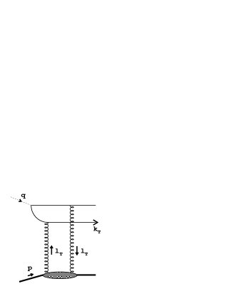
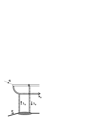
Figure 2: The diffractive $q\bar{q}$ and $q\bar{q}g$ contributions to $F_{2}^{D(3)}$.

Following the idea of the analysis [18], the diffractive structure function $F_{2}^{D(3)}$ is the sum of the three contributions shown in Fig. 2, the $q\bar{q}$ production from transverse and longitudinal photons, and the $q\bar{q}g$ production,

$$F_{2}^{D(3)}(\beta,Q^{2},x_{{I\!\!P}})\,=\,F^{T}_{q\bar{q}}\,+\,F^{L}_{q\bar{q}}\,+\,F^{T}_{q\bar{q}g}\,,$$ (18)

where $T$ and $L$ refer to the polarization of the virtual photon. For the $q\bar{q}g$ contribution only the transverse polarization is considered, since the longitudinal counterpart has no leading logarithm in $Q^{2}$. In this approach, the diffractive $q\bar{q}$ and $q\bar{q}g$ systems interact with the proton like in the two gluon exchange model. The coupling of the two gluons to the proton is effectively described the dipole cross section, determined from the analysis of inclusive DIS.

The computation of the diffractive structure functions in this case was presented in [28]. Here we quote only the final results. The transverse $q\bar{q}$ part is given by

$$F_{q\bar{q}}^{T}\,=\,\frac{3}{64\pi^{4}B_{D}\,x_{{I\!\!P}}}\;\sum_{f}e_{f}^{2}\;\frac{\beta^{2}}{(1-\beta)^{3}}\;\int_{0}^{\frac{Q^{2}(1-\beta)}{4\,\beta}}dk^{2}\;\frac{\displaystyle 1-\frac{2\beta}{1-\beta}\frac{k^{2}}{Q^{2}}}{\displaystyle\sqrt{1-\frac{4\beta}{1-\beta}\frac{k^{2}}{Q^{2}}}}\;\;\phi_{1}^{2}(k,\beta,x_{{I\!\!P}})\,,$$ (19)

and the longitudinal $q\bar{q}$ contribution takes the form

$$F_{q\bar{q}}^{L}\,=\,\frac{3}{16\pi^{4}B_{D}\,x_{{I\!\!P}}}\;\sum_{f}e_{f}^{2}\;\frac{\beta^{3}}{(1-\beta)^{4}}\;\int_{0}^{\frac{Q^{2}(1-\beta)}{4\,\beta}}dk^{2}\;\frac{\displaystyle{k^{2}}/{Q^{2}}}{\displaystyle\sqrt{1-\frac{4\beta}{1-\beta}\frac{k^{2}}{Q^{2}}}}\;\;\phi_{0}^{2}(k,\beta,x_{{I\!\!P}})\,,$$ (20)

where the “impact factors” $\phi_{i=0,1}$ read

$$\phi_{i}(k,\beta,x_{{I\!\!P}})\;=\;k^{2}\,\int_{0}^{\infty}dr\,r\,K_{i}\!\left(\sqrt{\frac{\beta}{1-\beta}}kr\!\right)\,J_{i}(kr)\;\hat{\sigma}(x_{{I\!\!P}},r)\;,$$ (21)

and $K_{i}$ and $J_{i}$ are the Bessel functions. The quoted formulae correspond to eqs. (32) and (33) in [28], respectively, with the angular integration already done, see also the second paper of [29] for a similar result. $B_{D}$ is the diffractive slope, present due to the integration over $t$ of $F^{D(4)}$ with the assumed $t$-dependence: $F^{D(4)}=\exp(B_{D}t)\,F^{D(3)}$. Its value is taken from the HERA experiments. The $k$-integration in eqs. (19) and (20) is performed over the transverse momentum of the quarks in the $q\bar{q}$ pair, $k=|{\bf k}_{\perp}|$. The final result depends on the squared “impact factors”, and thus on the square of the dipole cross section $\hat{\sigma}$.

One should realize that the longitudinal contribution is suppressed by a power of $Q^{2}$ in comparison to the transverse contribution, i.e. the longitudinal structure function is a higher twist contribution. Although of higher twist nature this contribution has some importance as will be seen later.

The leading twist part of the transverse structure function, which corresponds to the diffractive $q\bar{q}$ production, can be extracted from (19) by neglecting the factors with powers of $k^{2}/Q^{2}$ under the integral and taking the upper limit of the integration to infinity. Strictly speaking, energy conservation is violated in this case, but the corrections are of higher twist nature which in this case will be neglected because of their smallness. With the new limit the integral is still finite, and we can write the leading twist part of (19) as

$$F_{q\bar{q}}^{T(LT)}\,=\,\frac{3}{64\pi^{4}B_{D}\,x_{{I\!\!P}}}\;\sum_{f}e_{f}^{2}\;\frac{\beta^{2}}{(1-\beta)^{3}}\;\int_{0}^{\infty}dk^{2}\;\phi_{1}^{2}(k,\beta,x_{{I\!\!P}})\;.$$ (22)

A detailed analysis based on the dipole representation of the $q\bar{q}$ wave function shows that the approximation leading to eq. (22) corresponds to the aligned jet configuration of the $q\bar{q}$ pair in the proton rest frame. The smallness of the factor

$$\frac{\beta}{1-\beta}\,\frac{k^{2}}{Q^{2}}\,=\,\frac{k^{2}}{M^{2}}\,=\,z(1-z)$$ (23)

which we neglected in eq. (19) ($M$ is the diffractive mass and $z,\,(1-z)$ are the longitudinal momentum fractions of the final state quarks with respect to the photon momentum) means that one of the quarks takes almost the whole longitudinal photon momentum (e.g. $z\approx 1$) while the other quark forms the remnant with $(1-z)\approx 0$. Similar conclusions on the leading twist part of diffractive DIS have been drawn in ref. [26].

Now, we can determine the diffractive quark distributions according to eq. (12) (integrated over $t$),

$$F_{q\bar{q}}^{T(LT)}\,=\,2\,\sum_{f}e_{f}^{2}\;\beta\;q^{D}(\beta,Q^{2},x_{{I\!\!P}})$$ (24)

Hence the diffractive quark distribution is given by (independent of the quark flavour $f$)

$$q^{D}(\beta,Q^{2},x_{{I\!\!P}})\,\equiv\,x_{{I\!\!P}}{\cal{F}}^{D}_{q/p}(\beta,Q^{2},x_{{I\!\!P}})\,=\,\frac{3}{128\pi^{4}B_{D}\,x_{{I\!\!P}}}\;\frac{\beta}{(1-\beta)^{3}}\;\int_{0}^{\infty}dk^{2}\;\phi_{1}^{2}(k,\beta,x_{{I\!\!P}})\,,$$ (25)

Notice the lack of the $Q^{2}$-dependence on the r.h.s. of eq. (25). This may be viewed as a consequence of not having included ultraviolet divergent corrections which would require a cutoff. With those corrections the parton distributions become $\mu^{2}$-dependent, and evolution would relate the distributions at different $\mu^{2}$ values. Still, we may use the found diffractive quark distributions as the input distributions for the DGLAP evolution equations at some initial scale. Of course, the choice of the initial scale introduces an uncertainty for the prediction.

The detailed discussion of the $q\bar{q}g$ contribution can be found in [28] and [16] with the details of the calculations in the Appendix. The new contribution was computed assuming strong ordering in transverse momenta of the gluon and the $q\bar{q}$ pair, i.e. $k_{\perp g}\ll k_{\perp q}\approx k_{\perp\bar{q}}$. This assumption allows to treat the $q\bar{q}g$ system as a $g\bar{g}$ dipole in the transverse configuration space $\bf{r}$, where $\bf{r}$ is the Fourier conjugate variable to the quark transverse momentum $\bf{k}_{\perp}$.

The formula for the $q\bar{q}g$ diffractive structure function which we quote below corresponds to eq. (39) in [28], integrated over the azimuth angle in configuration space . Thus we have

$$F_{q\bar{q}g}^{T}(\beta,Q^{2},x_{{I\!\!P}}) = \frac{81\beta}{256\pi^{4}B_{D}\,x_{{I\!\!P}}}\;\sum_{f}e_{f}^{2}\;\;\frac{\alpha_{s}}{2\pi}\;\int_{\beta}^{1}\frac{d{\beta}^{\prime}}{{\beta}^{\prime}}\left[\left(1-\frac{\beta}{{\beta}^{\prime}}\right)^{2}+\left(\frac{\beta}{{\beta}^{\prime}}\right)^{2}\right]$$

$$\times \frac{{\beta}^{\prime}}{(1-{\beta}^{\prime})^{3}}\;\int_{0}^{Q^{2}(1-{\beta}^{\prime})}dk^{2}\;\log\left(\frac{Q^{2}(1-{\beta}^{\prime})}{k^{2}}\right)\;\phi_{2}^{2}(k,{\beta}^{\prime},x_{{I\!\!P}})\;,$$

where the impact factor $\phi_{2}$ is given by eq. (21) with $i=2$. The variable ${\beta}^{\prime}$ describes the momentum fraction of the $t$-channel exchanged gluon with respect to the pomeron momentum $x_{{I\!\!P}}p$. The combination $k^{2}/(1-{\beta}^{\prime})$ which enters the logarithm is its mean virtuality, and $k=|{\bf k}_{\perp}|$ is the transverse momentum of the final state gluon. The term in square brackets under the first integral is the Altarelli-Parisi splitting function for $g\rightarrow qq$, which results from the approximation that the transverse momentum of the emitted gluon is smaller than transverse momenta of the quarks.

The diffractive gluon distribution can be found from eq. (3). In the calculation of this contribution strong ordering between the gluon and quark transverse momenta was assumed. In this approximation the integration over the transverse momentum of the quark loop gives a logarithmic contribution which has a natural lower cutoff, the virtuality of the gluon $k^{2}/(1-{\beta}^{\prime})$. At the same time the virtuality of the gluon should not exceed $Q^{2}$. This is the origin of the logarithmic term in (3). Collinear factorization means that we can pull that logarithm out of the integral over the gluon transverse momenta, and add to it an arbitrary initial scale $Q_{0}^{2}<Q^{2}$. Thus we can write

$$F_{q\bar{q}g}^{T}\,=\,2\,\sum_{f}e_{f}^{2}\;\beta\,\left\{\frac{\alpha_{s}}{2\pi}\;\log\frac{Q^{2}}{Q_{0}^{2}}\;\int_{\beta}^{1}\frac{d{\beta}^{\prime}}{{\beta}^{\prime}}\;\frac{1}{2}\left[\left(1-\frac{\beta}{{\beta}^{\prime}}\right)^{2}+\left(\frac{\beta}{{\beta}^{\prime}}\right)^{2}\right]\,x_{{I\!\!P}}{\cal{F}}_{g/p}^{D}({\beta}^{\prime},x_{{I\!\!P}})\right\}\,,$$ (27)

where the diffractive gluon distribution is given by

$$g^{D}({\beta},x_{{I\!\!P}})\,\equiv\,x_{{I\!\!P}}{\cal{F}}_{g/p}^{D}({\beta},x_{{I\!\!P}})\;=\;\frac{81}{256\pi^{4}B_{D}\,x_{{I\!\!P}}}\;\frac{{\beta}}{(1-{\beta})^{3}}\;\int_{0}^{\infty}dk^{2}\;\phi_{2}^{2}(k,{\beta},x_{{I\!\!P}})\,$$ (28)

and $\phi_{2}$ is given by eq. (21) with $i=2$. As in the case of the quark distribution (25), the found gluon distribution does not depend on $Q^{2}$, and serves as the initial distributions at some fixed scale $Q_{0}^{2}$.

The motivation for the above identification of the diffractive gluon distributions is the structure in the curly brackets on the r.h.s of eq. (27). It is identical to the structure resulting from the DGLAP evolution with one splitting of the gluon into a $q\bar{q}$ pair.

Figure 3: Diffractive quark (25) and gluon (28) distributions (multiplied by $x=x_{I\!\!P}\,\beta$) based on the saturation model as a function of $\beta$ for $x_{{I\!\!P}}=0.0042$ at the initial scale $Q_{0}^{2}$.

The combined initial parton distributions (25) and (28) ( depicted in Fig.3 ) allow a complete description of the leading twist part of diffractive DIS by serving as the initial conditions for the DGLAP evolution equations. DGLAP evolution means that our diffractive system becomes more complicated due to additional parton emissions.

The longitudinal, higher twist contribution requires a separate treatment. It becomes important for large values of $\beta$, where the $q\bar{q}$ and the $q\bar{q}g$ production from transverse photons is negligible [28, 16, 18]. In our present analysis we simply add this contribution to the evolved leading twist part. The complete expression of the structure function reads

$$F_{2}^{D(3)}\,=\,F_{2}^{D(3)(LT)}\,+\,F_{q\bar{q}}^{L}\,.$$ (29)

where $F_{2}^{D(3)LT}$ is given by

$$F_{2}^{D(3)(LT)}\,=\,2\,\sum_{f}e_{f}^{2}\;\beta\;q^{D}(\beta,Q^{2},x_{{I\!\!P}})\,,$$ (30)

with the full DGLAP evolution. $F_{q\bar{q}}^{L}$ is given by eq. (20).

In the following we present a comparison of the description based on eq. (29) with the diffractive data from HERA. Before doing that we briefly discuss $x_{{I\!\!P}}$-factorization.

4 The issue of Regge factorization

Up to now, we have not made use of the particular form (17) of the dipole cross section $\hat{\sigma}$. We only implicitly assumed that the integrals involving $\hat{\sigma}$ are finite. The scaling property, i.e. that $\hat{\sigma}$ is a function of the dimensionless ratio $r/R_{0}(x)$, has the remarkable consequence that the $x_{{I\!\!P}}$-dependent part of the found diffractive parton distributions (DPD) factorizes.

Introducing the dimensionless variables $\hat{k}=kR_{0}(x)$ and $\hat{r}=r/R_{0}(x)$ in (25) and (28) and assuming $Q_{0}^{2}$ to be a fixed scale, we find the following factorized form

$$q^{D}(\beta,x_{{I\!\!P}}) = \frac{1}{x_{{I\!\!P}}R_{0}^{2}(x_{{I\!\!P}})}\;f_{q/{I\!\!P}}(\beta)\,,$$ (31)

$$g^{D}(\beta,x_{{I\!\!P}}) = \frac{1}{x_{{I\!\!P}}R_{0}^{2}(x_{{I\!\!P}})}\;f_{g/{I\!\!P}}(\beta)\,.$$ (32)

We have introduced a notation similar to that in (13) for the $\beta$-dependent factors. This type of factorization looks like Regge factorization but has nothing to do with Regge theory. It merely results from the scaling properties of the saturating cross section $\hat{\sigma}$. Since the evolution does not affect the $x_{{I\!\!P}}$-dependence of the DPD, the factorized form will be valid for any scale $Q^{2}$.

Now, we can rewrite eq. (30) as

$$F_{2}^{D(3)(LT)}\,=\,\frac{1}{x_{{I\!\!P}}R_{0}^{2}(x_{{I\!\!P}})}\,2\,\sum_{f}e_{f}^{2}\;\beta\,f_{q/{I\!\!P}}(\beta,Q^{2})\,$$ (33)

in which the $x_{{I\!\!P}}$-dependence is factored out. In the saturation model ($R_{0}(x)\sim x^{\lambda/2}$) the parameter $\lambda=0.29$ was determined from a fit to inclusive DIS data only [27]. The same value holds for diffractive interactions, thus we find a definite prediction for the $x_{{I\!\!P}}$-dependence of the leading twist diffractive structure function

$$F_{2}^{D(3)(LT)}\,\sim\,x_{{I\!\!P}}^{-1-\lambda}\,.$$ (34)

At present, the bulk of diffractive data in DIS support the factorized form (34). They are usually interpreted [1, 2] in terms of the $t$-averaged pomeron intercept $\overline{\alpha_{I\!\!P}}$, i.e.

$$F_{2}^{D(3)}\,\sim\,x_{{I\!\!P}}^{1-2\,\overline{\alpha_{I\!\!P}}}\,.$$ (35)

Such a dependence has been introduced in the spirit of the Ingelman-Schlein model (15), with the $t$-integration performed, $F_{2}^{D(3)}\sim\int dt\,f(x_{{I\!\!P}},t)\sim x_{{I\!\!P}}^{1-2\,\overline{\alpha_{I\!\!P}}}$. Thus, according to (34) and (35) we find

$$\overline{\alpha_{I\!\!P}}\,=\,\frac{\lambda}{2}+1\,\approx\,1.15\,,$$ (36)

which is in remarkable agreement with the values found at HERA, $\overline{\alpha_{I\!\!P}}=\alpha_{I\!\!P}(0)-0.03=1.17$ by H1 [1] and $\overline{\alpha_{I\!\!P}}=1.13$ by ZEUS [2].

Summarizing, the leading twist description extracted from the saturation model of DIS diffraction leads to the factorization of the $x_{{I\!\!P}}$-dependent part of the cross section similar to Regge factorization. It correctly predicts the value of the “effective pomeron intercept”. The $Q^{2}$-dependence of the diffractive structure function does not affect the $x_{{I\!\!P}}$-factorization. This means that the saturation model for the dipole cross section gives effectively the result which coincides with the Regge approach to DIS diffraction, although the physics behind is completely different. The relative hardness of the intrinsic scale $1/R_{0}(x_{{I\!\!P}})\sim 1~{}\mbox{\rm GeV}$ in the saturation model suggests that DIS diffraction is a semihard process rather than a soft process as Regge theory would require.

In the presented description, the leading twist structure function vanishes when $\beta\rightarrow 1$, i.e. for small diffractive mass $M^{2}\ll Q^{2}$. This is not the case for the higher twist longitudinal contribution $F_{Lq\bar{q}}^{D}$ , eq. (20), which dominates in the region of $\beta\approx 1$ [18]. The expected $x_{{I\!\!P}}$-dependence for this contribution is given by

$$F_{q\bar{q}}^{L}\,\sim\,\frac{1}{x_{{I\!\!P}}R^{4}_{0}(x_{{I\!\!P}})}\,\sim\,x_{{I\!\!P}}^{-1-2\lambda}\,,$$ (37)

which clearly violates the universality of the effective pomeron intercept, assumed in the Ingelman-Schlein model. The first indication of this effect is observed at HERA by measuring the effective pomeron intercept in different regions of the diffractive mass as a function of $Q^{2}$ [2]. The intercept seems to be bigger for smaller diffractive masses ($\beta\rightarrow 1$), and the description based on perturbative QCD gives a satisfactory explanation [28].

5 Comparison with data

In this section we present a comparison of the leading twist part of diffractive DIS including DGLAP evolution plus the corresponding longitudinal twist-4 component (eq. (29)) with the diffractive data from the HERA experiments.

In Fig. 3 we show the quark and gluon diffractive distributions at some initial scale $Q_{0}^{2}$. This scale, however, is not determined in this approach. Thus, it can be treated as a phenomenological parameter which may be tuned to obtain the best description of the DIS diffractive data. We tried various options and found that $Q_{0}^{2}\approx 1.5~{}\mbox{\rm GeV}^{2}$ is the best choice for this purpose. We used the leading logarithmic evolution equations with three massless flavours, and the value of $\Lambda_{QCD}=200~{}\mbox{MeV}$ in $\alpha_{s}$.

Fig. 4 shows the results of our studies with data from H1 and Fig. 5 data from ZEUS. The dashed lines represent the total contribution according to eq. (29). The pure leading twist structure function $F_{2}^{D(3)LT}$ with the leading DGLAP evolution is shown by the dotted lines. The difference (if visible) between the dashed and dotted lines is the effect of the longitudinal twist-4 component $F^{L}_{q\bar{q}}$ added into the leading twist result. As expected, the twist-4 component is significant in the large-$\beta$ domain, see also [18] for a detailed discussion. Notice the change of the slope in $x_{{I\!\!P}}$ when the twist-4 component is added. The overall agreement between the data and the model (29) is reasonably good, taking into account the fact that the only tuned parameter is the initial scale for the evolution $Q^{2}_{0}$. The parameters of the evolution equations are standard, and the diffractive slope $B_{D}=6~{}\mbox{\rm GeV}^{-2}$ which effects the normalization is taken from the measurements as in the analysis [28]. The significance of the twist-4 contribution at large $\beta$ is clearly demonstrated.

Looking at Fig. 4 and 5, we realize that at large $\beta$ and $Q^{2}$ the agreement between the data and the model with evolution starts to deteriorate. The reason for this is illustrated in Fig. 6 where we show $F_{2}^{D}$ for fixed value of $x_{{I\!\!P}}=0.0042$ as a function of $\beta$, for different values of $Q^{2}$. The DGLAP evolution depopulates the region of large $\beta$, shifting the parton distributions towards smaller values of $\beta$ (compare the dotted lines showing the initial distributions and the dashed lines showing the evolved distributions). The twist-4 component $F^{L}_{q\bar{q}}$ (the difference between the solid and the dashed lines) largely compensates for this effect. Its significance, however, diminishes as $Q^{2}$ rises due to the $1/Q^{2}$ dependence of twist-4.

There are at least two effects which may enhance $F^{L}_{q\bar{q}}$ when $Q^{2}$ rises, thus accounting for the difference between the data and the discussed description. In principle, twist-4 should also have logarithmic evolution, in addition to the $1/Q^{2}$ dependence, which could push $F^{L}_{q\bar{q}}$ into the right direction. Unfortunately, this aspect is beyond the scope of the present paper. Another effect which is important at large $\beta$ is skewedness of the diffractive parton distributions, see [40] for a recent discussion and references therein. This effect is known to enhance $F_{q\bar{q}}^{T,L}$ at large $\beta$. Since the enhancement rises with $Q^{2}$, the skewedness may account for the discussed difference between the data and their description in the region of large $\beta$ and $Q^{2}$.

6 Conclusions

We have reviewed the description of diffractive deep inelastic scattering in the light of the collinear factorization theorem. This theorem applies to the leading twist terms of the cross section and introduces the notion of diffractive parton distributions. We have extracted a precise analytic form for these distributions from the approach in which the diffractive state is formed by the $q\bar{q}$ and $q\bar{q}g$ systems, computed in pQCD. The convolution with a dipole cross section from the saturation model leads to the $x_{{I\!\!P}}$-factorization of the diffractive structure functions, similar to Regge factorization, which correctly describe the energy dependence found at HERA by the H1 and ZEUS collaborations. We further evolved the diffractive parton distributions with the DGLAP evolution equations and pointed out the significance of the twist-4 component at large $\beta$ for the agreement with the data. The latter was originally advocated in [18] and originates from the longitudinal $q{\bar{q}}$ contribution. The twist-4 component breaks the universality of the effective $x_{{I\!\!P}}$-dependence, making it stronger at large $\beta$. This stays in contrast to the assumed universality in the Ingelman-Schlein model. Finally, we suggest some necessary modifications of the description at large $\beta$ and $Q^{2}$ to improve the agreement with the data in this kinematic region.

Acknowledgements

We thank Jochen Bartels and Henri Kowalski for useful discussions and critical reading of the manuscript. K.G.-B. thanks Deutsche Forschungsgemeinschaft for financial support. This research has been supported in part by the EU Fourth Framework Programme “Training and Mobility of Researchers” Network, “Quantum Chromodynamics and the Deep Structure of Elementary Particles”, contract FMRX-CT98-0194 (DG 12-MIHT) and by the Polish KBN grant No. 5 P03B 144 20.

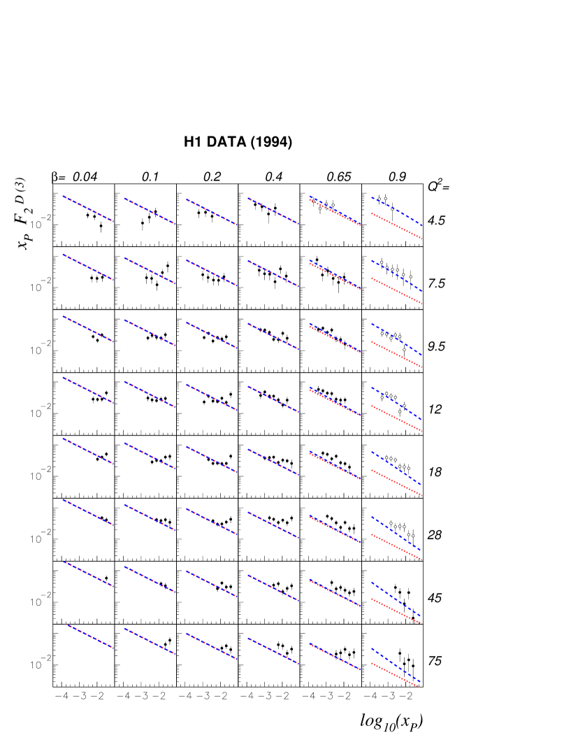
Figure 4: The comparison with H1 data [1]. The dashed lines correspond to the leading twist contribution with the twist-4 component added, eq. (29). The leading twist contribution is shown by the dotted lines.

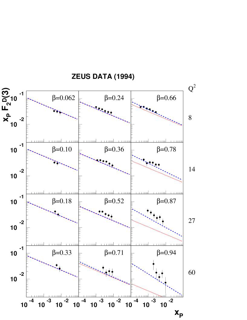
Figure 5: The comparison with ZEUS data [2]. The dashed lines correspond to the leading twist contribution with the twist-4 component added, eq. (29). The leading twist contribution is shown by the dotted lines.

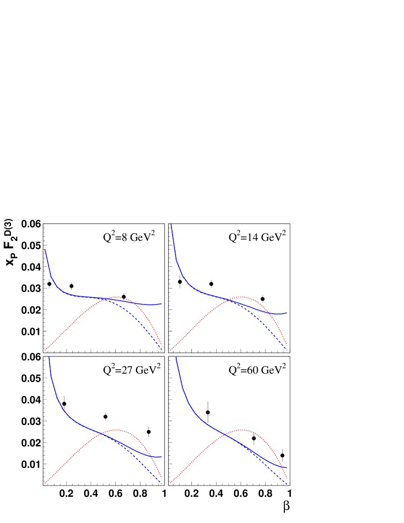
Figure 6: The effect of the DGLAP evolution in $Q^{2}$. The dotted lines show the leading twist structure function at the initial scale $Q_{0}^{2}=3~{}\mbox{\rm GeV}^{2}$. The dashed lines correspond to evolved structure function at the indicated values of $Q^{2}$. The solid line is the sum of the evolved leading twist contribution and twist-4 component, eq. (29). The ZEUS data at $x_{{I\!\!P}}=0.0042$ are shown.

References

- [1] H1 Collaboration, C. Adloff et al., Z. Phys. C76 (1997) 613.
- [2] ZEUS Collaboration, M. Derrick et al., Eur. Phys. J. C6 (1999) 43.
- [3] M. Wüsthoff and A.D. Martin, J. Phys. G25 (1999) R309.
- [4] A. Hebecker, Phys. Rep. 331 (2000) 1; Acta Phys. Polon. B30 (1999) 3777.
- [5] H. Abramowicz, in Proc. of the 19th Intl. Symp. on Photon and Lepton Interactions at High Energy LP99 ed. J.A. Jaros and M.E. Peskin, eConfC990809, 495 (2000), hep-ph/0001054.
- [6] G. Ingelman and P. Schlein, Phys. Lett. B152 (1985) 256.
- [7] C. Royon et al., hep-ph/0010015.
-
[8]
K. Golec–Biernat and J. Kwieciński,
Phys. Lett. B353 (1995) 329;
T. Gehrmann and W. J. Stirling, Z. Phys. C70 (1996) 89;
A. Capella, A. Kaidalov, C. Merino and J. Tran Thanh Van, Phys. Rev. D53 (1996) 2309;
K. Golec–Biernat and J. Kwieciński, Phys. Rev. D55 (1997) 3209;
K. Golec–Biernat, J. Kwieciński and A. Szczurek, Phys. Rev. D56 (1997) 3955;
L. Alvero, J.C. Collins, J. Terron and J. Whitmore, Phys. Rev. D59 (1999) 074022. - [9] A. Berera and D.E. Soper, Phys. Rev. D50 (1994) 4328.
- [10] L. Trentadue and G. Veneziano, Phys. Lett. 323 (1994) 201.
-
[11]
Z. Kunszt and W.J. Stirling, hep-ph/9609245;
A. Berera and D.E. Soper, Phys. Rev. D53 (1996) 6162. - [12] J. C. Collins, Phys. Rev. D57 (1998) 3051, Erratum-ibid. D61 (2000) 019902.
- [13] J. C. Collins, L. Frankfurt and M. Strikman Phys. Lett. B307 (1993) 161.
- [14] N.N. Nikolaev and B.G. Zakharov, Z. Phys. C53 (1992) 331.
- [15] J. Bartels, H. Lotter and M. Wüsthoff, Phys. Lett. B379 (1996) 239, Erratum-ibid. B382 (1996) 449;
-
[16]
E. Levin and M. Wüsthoff,
Phys. Rev. D50 (1994) 4306;
M. Wüsthoff, Phys. Rev. D56 (1997) 4311. - [17] N.N. Nikolaev and B.G. Zakharov, Z. Phys. C64 (1994) 631.
- [18] J. Bartels, J. Ellis, H. Kowalski and M. Wüsthoff, Eur. Phys. J. C7 (1999) 443.
- [19] J. Bartels, H. Jung and M. Wüsthoff, Eur. Phys. J. C11 (1999) 111.
- [20] M.G. Ryskin, Sov. J. Nucl. Phys. 52 (1990) 529.
- [21] J. Bartels and M. Wüsthoff, J. Phys. G22 (1996) 929.
- [22] F. Hautmann, Z. Kunszt and D. E. Soper, Phys. Rev. Lett. 81 (1998) 3333; Nucl. Phys. Proc. Suppl. 79 (1999) 260.
- [23] J. Bartels and M. Wüsthoff, Z. Phys. C66 (1995) 157.
-
[24]
M. Genovese, N.N Nikolaev and B.G.Zakharov,
JETP 81 (1995) 625;
A. Białas and R. Peschanski, Phys. Lett. B378 (1996) 302; ibid. B387 (1996) 405;
A. Bialas Acta Phys. Polon. B28 (1997) 1239;
A. Bialas and W. Czyz, Acta Phys.Polon. B29 (1998) 2095;
S. Munier, R. Peschanski and C. Royon, Nucl. Phys. B534 (1998) 297. -
[25]
W. Buchmüller and A. Hebecker,
Nucl. Phys. B476 (1996) 203;
W. Buchmüller, M.F. McDermott and A. Hebecker, Nucl. Phys. B487 (1997) 283, Erratum-ibid. B500 (1997) 621;
W. Buchmuller, T. Gehrmann and A. Hebecker, Nucl. Phys. B537 (1999) 477. - [26] A. Hebecker, Nucl. Phys. B505 (1997) 349.
- [27] K. Golec–Biernat and M. Wüsthoff, Phys. Rev. D59 (1999) 014017.
- [28] K. Golec–Biernat and M. Wüsthoff, Phys. Rev. D60 (1999) 114023.
- [29] J. R. Forshaw, G. Kerley and G. Shaw, Phys. Rev D60 (1999) 074012, Nucl. Phys. A675 (2000) 80.
- [30] E. Gotsman, E. Levin, U. Maor and E. Naftali, Eur. Phys. J. C10 (1999) 689; hep-ph/0007261; hep-ph/0010198.
- [31] M. McDermott, L. Frankfurt, V. Guzey and M. Strikman, Eur. Phys. J. C16 (2000) 641.
-
[32]
Ia. Balitsky, Nucl.Phys. B463 (1996) 99;
Y.V. Kovchegov, Phys. Rev. D60 (1999) 034008; Phys. Rev. D61 (2000) 074018;
G. Levin and K. Tuchin, Nucl. Phys. B537 (2000) 833;
M.A. Braun, Eur. Phys. J. C16 (2000) 337. -
[33]
Y.V. Kovchegov and A.H. Mueller, Nucl. Phys. B529 (1998) 451;
Y.V. Kovchegov and L. McLerran, Phys. Rev. D60 (1999) 054025; Erratum-ibid. D62 (2000) 019901;
Y.V. Kovchegov and G. Levin, Nucl. Phys. B577 (2000) 221; -
[34]
J. Jalilian-Marian, A. Kovner, L. McLerran and H.
Weigert, Phys. Rev. D55 (1997) 5414;
J. Jalilian-Marian, A. Kovner and H. Weigert, Phys. Rev. D59 (1999) 014014; Phys. Rev. D59 (1999) 014015; Phys. Rev. D59 (1999) 034007; Erratum-ibid. D59 (1999) 099903;
A. Kovner, J.Guilherme Milhano and H. Weigert, Phys. Rev. D62 (2000) 114005;
H. Weigert, NORDITA-2000-34-HE, hep-ph/0004044;
E. Iancu, A. Leonidov and L. McLerran, hep-ph/0102009. -
[35]
L.V. Gribov, E.M. Levin and M.G. Ryskin, Phys. Rep.
100 (1983) 1;
A.H. Mueller and Jian-wei Qiu, Nucl. Phys. B268 (1986) 427;
L. McLerran and R. Venugopalan, Phys. Rev. D49 (1994) 2233, D49 (1994) 3352, D50 (1994) 2225;
R. Venugopalan, Acta Phys. Polon. B30 (1999) 3731. - [36] A. Donnachie and P.V. Landshoff, Nucl. Phys. B 231 (1984) 189.
- [37] A. Donnachie and P.V. Landshoff, Phys. Lett. B 296 (1992) 227.
- [38] A. Donnachie and P.V. Landshoff, Phys. Lett B191 (1987) 309; Nucl. Phys. B303 (1988) 634.
- [39] A. Staśto, K. Golec-Biernat and J. Kwieciński, Phys. Rev. Lett. 86 (2001) 596.
- [40] A. Hebecker and T. Teubner, Phys. Lett. B498 (2001) 16.