Physics Implications of Precision Electroweak Experiments

Abstract

A brief review is given of precision electroweak physics, and its implications for establishing the standard model and constraining the possibilities for new physics at the TeV scale and beyond.

Abstract

A brief review is given of precision electroweak physics, and its implications for establishing the standard model and constraining the possibilities for new physics at the TeV scale and beyond.

1 Historical Perspective

The weak neutral current (WNC) and the closely related $W$ and $Z$ properties have always been the primary prediction and test of electroweak unification [1]. Following the original discovery of the WNC in 1973, there were successive generations of more and more precise experiments, culminating in the high precision $Z$ pole experiments at LEP and SLC in the 1990s and the high energy LEP 2. The overall result is that:

• The standard model (SM) is correct and unique to first approximation, establishing the gauge principle as well as the SM gauge group and representations.

• The SM is correct at loop level. This confirms the basic principles of renormalizable gauge theory, allowed the successful prediction of $m_{t}$ and $\alpha_{s}$, and strongly constrains $M_{H}$.

• New physics at the TeV scale is severely constrained, with the ideas of unification strongly favored over TeV-scale compositeness.

• The precisely measured gauge couplings are consistent with (supersymmetric) gauge unification.

The verification of electroweak unification went through a number of phases. The first was the discovery of WNC processes in the Gargamelle bubble chamber at CERN and the HPW experiment at Fermilab in 1973. The WNC was a critical prediction of $SU(2)\mbox{$\times$}U(1)\$unification, which had been proposed independently by Weinberg and Salam a few years before, and recently shown to be renormalizable. Charged current (WCC) processes, as described by the Fermi theory, and QED were incorporated into the theory but not predicted. However, they were improved and justified, in that it became possible to calculate meaningful radiative corrections to $\mu$ decay and other processes. The original $SU(2)\mbox{$\times$}U(1)\$theory of leptons was successfully extended to hadronic processes with the introduction of the charm quark (the Glashow-Iliopoulos-Maiani (GIM) mechanism), which was observed in 1974. The period saw the simultaneous parallel development of quarks and QCD.

The next generation of experiments, during the late 1970’s, were typically of 10% precision [2]. They included purely WNC processes, such as $\mbox{$\stackrel{{\scriptstyle(-)}}{{\nu}}$}N\mbox{$\rightarrow$}\mbox{$\stackrel{{\scriptstyle(-)}}{{\nu}}$}N$ (elastic), $\mbox{$\stackrel{{\scriptstyle(-)}}{{\nu}}$}N\mbox{$\rightarrow$}\mbox{$\stackrel{{\scriptstyle(-)}}{{\nu}}$}X$ (inelastic), and $\mbox{$\stackrel{{\scriptstyle(-)}}{{\nu}}$}_{\mu}e\mbox{$\rightarrow$}\mbox{$\stackrel{{\scriptstyle(-)}}{{\nu}}$}_{\mu}e$, as well as reactor $\bar{\nu}_{e}e\mbox{$\rightarrow$}\bar{\nu}_{e}e$, for which there are both WNC and WCC contributions. In addition, the interference of WNC and photon exchange effects was observed in the polarization asymmetry in $eD\mbox{$\rightarrow$}eX$ at SLAC. This was crucial because it excluded pure $S$, $P$, and $T$ neutral current amplitudes (there was a confusion theorem that, in the absence of interference, any pure $V$ and $A$ amplitude could be mimicked by a combination of $S$, $P$, and $T$), as well as some versions of left-right symmetric $SU(2)_{L}\mbox{$\times$}SU(2)_{R}\mbox{$\times$}U(1)\$ models. The latter had been devised to explain early searches for WNC parity violation in heavy atoms, which (erroneously) did not observe any effects.

A number of issues had become important for the interpretation of the experiments. For example, they were sufficiently precise to require QCD corrections for the analysis of the deep inelastic neutrino scattering. Furthermore, the complementarity of experiments became increasingly evident: there were many types of experiments, probing different WNC couplings in different kinematic ranges. No one experiment was sensitive to all types of new physics, and in most cases the new physics effects in a given experiment could be hidden by a shift in the apparent value of the weak angle $\sin^{2}\theta_{W}\,$measured in that process. This led to the need for a global analysis: the experiments together provided much more information than individually. By examining their consistency and whether they implied a common value for $\sin^{2}\theta_{W}\,$one could test the SM and could separately determine the various WNC couplings in a more general analysis that did not assume the validity of the SM. Furthermore, a global analysis permitted the uniform and consistent application of the best possible theoretical treatments of all similar experiments, and allowed the proper treatment of common experimental and theoretical uncertainties and their correlations. On the other hand, combining experimental results in a global analysis requires a careful evaluation of systematic uncertainties, since either underestimations or overestimations can affect the results.

The global analyses made possible the model independent fits to WNC data. These allowed almost arbitrary ($V-A$ neutrino couplings and family-independent couplings were generally assumed) vector and axial vector effective four-fermion $\nu e$, $\nu q$, and $eq$ WNC interactions, and therefore parametrized the most general family-universal gauge theories involving left-handed neutrinos. The result was that the four-fermi interactions predicted by the standard model are correct to first approximation, eliminating a number of competing gauge models which predicted completely different interactions. Of course, perturbations around these results, due to new physics, were still allowed. Furthermore, the new tree-level parameter $\sin^{2}\theta_{W}\,$of the SM was determined to be $\sin^{2}\theta_{W}\,$= 0.229 $\pm 0.010$. There were also limits on $\rho-1$, which parametrizes sources of $SU(2)$ breaking such as non-standard Higgs fields or fermion-doublet splittings. In modern language, this corresponded to a limit $m_{t}<290$ GeV.

The third generation of experiments [3, 4] began in the 1980’s, and continues with WNC experiments even to the present. They were typically of order 1–5% precision. They included pure weak $\nu N$ and $\nu e$ scattering processes, as well as weak-electromagnetic interference processes such as polarized $e^{\uparrow\downarrow}D$ or $\mu N$, $e^{+}e^{-}$$\rightarrow$ (hadron or charged lepton) cross sections and asymmetries below the $Z$ pole, and parity-violating effects in heavy atoms (APV). The APV experiments had resolved the experimental difficulties in the earlier generation, and the most precise involved the hydrogen-like $Cs$ atom, for which one could cleanly calculate the atomic matrix elements needed to interpret the results. This generation also included the direct observation and mass measurements of the $W$ and $Z$, which were discovered by UA1 and UA2 at CERN in 1983. The $Z$ mass in particular allowed the exclusion of contrived imitator models which had the same four-fermi operators as the SM, but very different $Z$ spectra.

The increased precision required refined theoretical inputs. Electroweak radiative corrections had to be included in the theoretical expressions, and with them one had to worry about alternative definitions of the renormalized $\sin^{2}\theta_{W}\,$. The most precise results (prior to the $Z$-pole era) involved deep inelastic scattering. This required careful consideration of the nucleon structure functions and their QCD evolution, including a reanalysis of all of the deep-inelastic neutrino experiments using common structure functions [3]. The most precise data involved the ratio of WNC/WCC scattering on heavy targets that were close to isoscalar, for which most of the strong interaction uncertainties canceled. The largest residual uncertainty was $c$ quark production in the WCC denominator. Fortunately, this could be measured and parametrized independently in dimuon production. Finally, considerable effort was needed in finding useful parametrizations of such classes of new physics and their effects as heavy $Z^{\prime}$ bosons, or new fermions with exotic weak interactions (e.g., involving right-handed fields in weak doublets, or left-handed singlets). It was important that the parametrizations apply to broad classes of models, but nevertheless that they be simple enough that they could be easily handled in fits.

The implications of these experimental and theoretical efforts were:

• The SM is correct to first approximation. That is, the four-fermion operators for $\nu q$, $\nu e$, and $eq$ were uniquely determined, in agreement with the standard model, and the $W$ and $Z$ masses agreed with the expectations of the $SU(2)\mbox{$\times$}U(1)\$gauge group and canonical Higgs mechanism, eliminating contrived imitators.

• Electroweak radiative corrections were necessary for the agreement of theory and experiment.

• The weak mixing angle (in the on-shell renormalization scheme) was determined to be $\sin^{2}\theta_{W}\,$= 0.229 $\pm 0.0064$, while consistency of the various observations, including radiative corrections, required $m_{t}<200$ GeV.

• Theoretical uncertainties, especially in the $c$ threshold in deep inelastic WCC scattering, dominated.

• The combination of WNC and WCC data uniquely determined the $SU(2)$ representations of all of the known fermions, i.e., of the $\nu_{e}$ and $\nu_{\mu}$, as well as the $L$ and $R$ components of the $e,\ \mu,\ \tau,\ d,\,s,\,b,\ u,$ and $c$ [5]. In particular, the left-handed $b$ was the lower component of an $SU(2)$ doublet, implying unambiguously that the $t$ quark had to exist. This was independent of theoretical arguments based on anomaly cancellation (which could have been evaded in alternative models involving a vector-like third family), and of constraints on the $t$ mass from electroweak loops.

• The electroweak gauge couplings were well-determined, allowing a detailed comparison with the gauge unification predictions of the simplest grand unified theories (GUT). It was found that ordinary $SU(5)\$was excluded (consistent with the non-observation of proton decay), but that the supersymmetric extension was allowed, i.e., that the data was “consistent with SUSY GUTS and perhaps even the first harbinger of supersymmetry” [3].

• There were stringent limits on new physics at the TeV scale, including additional $Z^{\prime}$ bosons, exotic fermions (for which both WNC and WCC constraints were crucial), exotic Higgs representations, leptoquarks, and new four-fermion operators.

In parallel with the WNC–$W$–$Z$, program, there were detailed studies of $\mu$ decay, which uniquely established its $V-A$ character, and of the rates and other observables in superallowed and neutron $\beta$ decay [1]. These constrained such new physics as $SU(2)_{L}\mbox{$\times$}SU(2)_{R}\mbox{$\times$}U(1)\$ models, exotic fermions, and models involving scalar exchange. They also allowed precise determination of elements of the quark mixing (CKM) matrix and of its unitarity, thus constraining such effects as a fourth family with significant mixings. The same period witnessed new experimental confirmations of QCD, as well as experimental and theoretical developments (in the SM and extensions) in loop-induced processes such as $b\mbox{$\rightarrow$}s\gamma$ and, recently, the anomalous magnetic moment of the muon [6].

2 The LEP/SLC Era

The LEP/SLC era greatly improved the precision of the electroweak program. It allowed the differentiation between non-decoupling extensions to the SM (such as most forms of dynamical symmetry breaking and other types of TeV-scale compositeness), which typically predicted several % deviations, and decoupling extensions (such as most of the parameter space for supersymmetry), for which the deviations are typically 0.1%.

The first phase of the LEP/SLC program involved running at the $Z$ pole, $e^{+}e^{-}\rightarrow Z\rightarrow\ell^{+}\ell^{-},\ \ q\bar{q},$ and $\nu\bar{\nu}$. During the period 1989-1995 the four LEP experiments ALEPH, DELPHI, L3, and OPAL at CERN observed $\sim 2\times 10^{7}Z^{\prime}s$. The SLD experiment at the SLC at SLAC observed some $5\times 10^{5}$ events. Despite the much lower statistics, the SLC had the considerable advantage of a highly polarized $e^{-}$ beam, with $P_{e^{-}}\sim$ 75%. There were quite a few $Z$ pole observables, including:

• The lineshape: $M_{Z},\Gamma_{Z},$ and the peak cross section $\sigma$

• The branching ratios for $e^{+}e^{-},\ \mu^{+}\mu^{-},\ \tau^{+}\tau^{-},\ q\bar{q},\ c\bar{c},\ b\bar{b},$ and $s\bar{s}$. One could also determine the invisible width, $\Gamma({\rm inv})$, from which one can derive the number $N_{\nu}=2.985\pm 0.008$ of active (weak doublet) neutrinos with $m_{\nu}<M_{Z}/2$, i.e., there are only 3 conventional families with light neutrinos. $\Gamma({\rm inv})$ also constrains other invisible particles, such as light sneutrinos and the light majorons associated with some models of neutrino mass.

• A number of asymmetries, including forward-backward (FB) asymmetries; the $\tau$ polarization, $P_{\tau}$; the polarization asymmetry $A_{LR}$ associated with $P_{e^{-}}$; and mixed polarization-FB asymmetries.

The expressions for the observables are summarized in Appendix A, and the experimental values and SM predictions in Table 1. These combinations of observables could be used to isolate many $Z$-fermion couplings, verify lepton family universality, determine $\sin^{2}\theta_{W}\,$in numerous ways, and determine or constrain $m_{t}$, $\alpha_{s}$, and $M_{H}$. LEP and SLC simultaneously carried out other programs, most notably studies and tests of QCD, and heavy quark physics.

LEP 2 ran from 1995-2000, with energies gradually increasing from $\sim 140$ to $\sim 208$ GeV. The principal electroweak results were precise measurements of the $W$ mass, as well as its width and branching ratios (these were measured independently at the Tevatron); a measurement of $e^{+}e^{-}\mbox{$\rightarrow$}W^{+}W^{-}$ as a function of center of mass (CM) energy, which tests the cancellations between diagrams that is characteristic of a renormalizable gauge field theory, or, equivalently, probes the triple gauge vertices; stringent lower limits on the Higgs mass, and even hints of an observation at $\sim$ 115 GeV; limits on anomalous quartic gauge vertices; and searches for supersymmetric or other exotic particles.

In parallel with the LEP/SLC program, there were much more precise ($<$ 1%) measurements of atomic parity violation (APV) in cesium at Boulder, along with the atomic calculations and related measurements needed for the interpretation; precise new measurements of deep inelastic scattering by the NuTeV collaboration at Fermilab, with a sign-selected beam which allowed them to minimize the effects of the $c$ threshold and reduce uncertainties to around 1%; and few % measurements of $\mbox{$\stackrel{{\scriptstyle(-)}}{{\nu}}$}_{\mu}e$ by CHARM II at CERN. Although the precision of these WNC processes was lower than the $Z$ pole measurements, they are still of considerable importance: the $Z$ pole experiments are blind to types of new physics that do not directly affect the $Z$, such as a heavy $Z^{\prime}$ if there is no $Z-Z^{\prime}$ mixing, while the WNC experiments are often very sensitive. During the same period there were important electroweak results from CDF and D$\not{\!0}$ at the Tevatron, most notably a precise value for $M_{W}$, competitive with and complementary to the LEP 2 value; a direct measure of $m_{t}$, and direct searches for $Z^{\prime}$, $W^{\prime}$, exotic fermions, and supersymmetric particles. Many of these non-$Z$ pole results are summarized in Table 2.

Quantity	Group(s)	Value	Standard Model	pull
$M_{Z}$       [GeV]	LEP	$91.1876\pm 0.0021$	$91.1874\pm 0.0021$	$0.1$
$\Gamma_{Z}$        [GeV]	LEP	$2.4952\pm 0.0023$	$2.4963\pm 0.0016$	$-0.5$
$\Gamma({\rm had})$   [GeV]	LEP	$1.7444\pm 0.0020$	$1.7427\pm 0.0015$	—
$\Gamma({\rm inv})$    [MeV]	LEP	$499.0\pm 1.5$	$501.74\pm 0.15$	—
$\Gamma({\ell^{+}\ell^{-}})$ [MeV]	LEP	$83.984\pm 0.086$	$84.018\pm 0.028$	—
$\sigma_{\rm had}$     [nb]	LEP	$41.541\pm 0.037$	$41.479\pm 0.014$	$1.7$
$R_{e}$	LEP	$20.804\pm 0.050$	$20.743\pm 0.018$	$1.2$
$R_{\mu}$	LEP	$20.785\pm 0.033$	$20.743\pm 0.018$	$1.3$
$R_{\tau}$	LEP	$20.764\pm 0.045$	$20.788\pm 0.018$	$-0.5$
$A_{FB}(e)$	LEP	$0.0145\pm 0.0025$	$0.0165\pm 0.0003$	$-0.8$
$A_{FB}(\mu)$	LEP	$0.0169\pm 0.0013$		$0.3$
$A_{FB}(\tau)$	LEP	$0.0188\pm 0.0017$		$1.4$
$R_{b}$	LEP + SLD	$0.21653\pm 0.00069$	$0.21572\pm 0.00015$	$1.2$
$R_{c}$	LEP + SLD	$0.1709\pm 0.0034$	$0.1723\pm 0.0001$	$-0.4$
$R_{s,d}/R_{(d+u+s)}$	OPAL	$0.371\pm 0.023$	$0.3592\pm 0.0001$	$0.5$
$A_{FB}(b)$	LEP	$0.0990\pm 0.0020$	$0.1039\pm 0.0009$	$-2.5$
$A_{FB}(c)$	LEP	$0.0689\pm 0.0035$	$0.0743\pm 0.0007$	$-1.5$
$A_{FB}(s)$	DELPHI,OPAL	$0.0976\pm 0.0114$	$0.1040\pm 0.0009$	$-0.6$
$A_{b}$	SLD	$0.922\pm 0.023$	$0.9348\pm 0.0001$	$-0.6$
$A_{c}$	SLD	$0.631\pm 0.026$	$0.6683\pm 0.0005$	$-1.4$
$A_{s}$	SLD	$0.82\pm 0.13$	$0.9357\pm 0.0001$	$-0.4$
$A_{LR}$ (hadrons)	SLD	$0.15138\pm 0.00216$	$0.1483\pm 0.0012$	$1.4$
$A_{LR}$ (leptons)	SLD	$0.1544\pm 0.0060$		$1.0$
$A_{\mu}$	SLD	$0.142\pm 0.015$		$-0.4$
$A_{\tau}$	SLD	$0.136\pm 0.015$		$-0.8$
$A_{e}(Q_{LR})$	SLD	$0.162\pm 0.043$		$0.3$
$A_{\tau}({\cal P}_{\tau})$	LEP	$0.1439\pm 0.0042$		$-1.0$
$A_{e}({\cal P}_{\tau})$	LEP	$0.1498\pm 0.0048$		$0.3$
$\bar{s}_{\ell}^{2}(Q_{FB})$	LEP	$0.2321\pm 0.0010$	$0.23136\pm 0.00015$	$0.7$

Table 1: Principal $Z$-pole observables, their experimental values, theoretical predictions using the SM parameters from the global best fit [7], and pull (difference from the prediction divided by the uncertainty). $\Gamma({\rm had})$, $\Gamma({\rm inv})$, and $\Gamma({\ell^{+}\ell^{-}})$ are not independent, but are included for completeness.

Quantity	Group(s)	Value	Standard Model	pull
$m_{t}$   [GeV]	Tevatron	$174.3\pm 5.1$	$174.2\pm 4.4$	$0.0$
$M_{W}$ [GeV]	LEP	$80.427\pm 0.046$	$80.394\pm 0.019$	$0.7$
$M_{W}$ [GeV]	Tevatron,UA2	$80.451\pm 0.061$		$0.9$
$R^{-}$	NuTeV	$0.2277\pm 0.0021\pm 0.0007$	$0.2301\pm 0.0002$	$-1.1$
$R^{\nu}$	CCFR	$0.5820\pm 0.0027\pm 0.0031$	$0.5834\pm 0.0004$	$-0.3$
$R^{\nu}$	CDHS	$0.3096\pm 0.0033\pm 0.0028$	$0.3093\pm 0.0002$	$0.1$
$R^{\nu}$	CHARM	$0.3021\pm 0.0031\pm 0.0026$		$-1.8$
$R^{\bar{\nu}}$	CDHS	$0.384\pm 0.016\pm 0.007$	$0.3862\pm 0.0002$	$-0.1$
$R^{\bar{\nu}}$	CHARM	$0.403\pm 0.014\pm 0.007$		$1.0$
$R^{\bar{\nu}}$	CDHS 1979	$0.365\pm 0.015\pm 0.007$	$0.3817\pm 0.0002$	$-1.0$
$g_{V}^{\nu e}$	CHARM II	$-0.035\pm 0.017$	$-0.0399\pm 0.0003$	—
$g_{V}^{\nu e}$	all	$-0.041\pm 0.015$		$-0.1$
$g_{A}^{\nu e}$	CHARM II	$-0.503\pm 0.017$	$-0.5065\pm 0.0001$	—
$g_{A}^{\nu e}$	all	$-0.507\pm 0.014$		$0.0$
$Q_{W}({\rm Cs})$	Boulder	$-72.65\pm 0.28\pm 0.34$	$-73.08\pm 0.04$	$1.0$
$Q_{W}({\rm Tl})$	Oxford,Seattle	$-114.8\pm 1.2\pm 3.4$	$-116.6\pm 0.1$	$0.5$
${\Gamma(b\rightarrow s\gamma)\over\Gamma(b\rightarrow ce\nu)}$	CLEO	$3.26^{+0.75}_{-0.68}\times 10^{-3}$	$3.15^{+0.21}_{-0.20}\times 10^{-3}$	$0.1$

Table 2: Recent non-$Z$-pole observables.

The LEP and (after initial difficulties) SLC programs were remarkably successful, achieving greater precision than had been anticipated in the planning stages, e.g., due to better than expected measurements of the beam energy (using a clever resonant depolarization technique) and luminosity. Credit goes to the individuals who built and operated the machines and computing systems, and to the experimenters who built, ran, and analyzed the results from the ALEPH, DELPHI, L3, OPAL (LEP) and SLD (SLC) detectors. The measurement of the $Z$ mass and width at LEP were so precise that the tidal effects of the moon, the levels of the water table and Lake Geneva, and electromagnetic effects from trains had to be taken into account. SLAC had an advantage of a high and well-measured $e^{-}$ polarization. (One regret is that LEP never implemented longitudinal polarization. The Blondel scheme would have permitted a high, self-calibrated polarization with its significant advantages.) The program was greatly enhanced by the efforts of the LEP Electroweak Working Group (LEPEWWG) [8], which combined the results of the four LEP experiments, and also those of SLD and some WNC and Tevatron results, taking proper account of common systematic and theoretical uncertainties, so that the maximum and most reliable information could be extracted.

A great deal of supporting theoretical effort was also essential. This included the calculation of the needed electromagnetic, electroweak, QCD, and mixed radiative corrections to the predictions of the SM [9, 10, 11]. Careful consideration of the competing definitions of the renormalized $\sin^{2}\theta_{W}\,$was needed. The principal theoretical uncertainty is the hadronic contribution $\Delta\alpha_{\rm had}^{(5)}(M_{Z})$ to the running of $\alpha$ from its precisely known value at low energies [12] to the $Z$-pole [13], where it is needed to compare the $Z$ mass with the asymmetries and other observables. The radiative corrections, renormalization schemes, and running of $\alpha$ are further discussed in Appendix B. Tremendous theoretical effort went into the development, testing, and comparison of radiative corrections packages such as ZFITTER, TOPAZ0, ALIBABA, BHLUMI, and GAPP, as well as other packages needed for the LEP 2 program. Finally, much effort went into the study of how various classes of new physics would modify the observables, and how they could most efficiently be parametrized.

Global analyses of the $Z$-pole and other data were carried out, e.g., by the LEPEWWG [8] and by Erler and myself for the Particle Data Group (PDG) [7], to test the consistency of the SM, determine its parameters, and search for or constrain new TeV-scale physics.

Although the $Z$-pole program has ended for the time being, there are prospects for future programs using the Giga-$Z$ option at TESLA or possible other linear colliders, which might yield a factor $10^{2}$ more events. This would enormously improve the sensitivity [14], but would also require a large theoretical effort to improve the radiative correction calculations [9, 11].

During the LEP/SLC era, the $Z$-pole, LEP 2, WNC, and Tevatron experiments successfully tested the SM at 0.1% level, including electroweak loops, thus confirming the gauge principle, SM group, representations, and the basic structure of renormalizable field theory. The standard model parameters $\sin^{2}\theta_{W}$, $m_{t}$, and $\alpha_{s}$ were precisely determined. In fact, $m_{t}$ was successfully predicted from its indirect loop effects prior to the direct discovery at the Tevatron, while the indirect value of $\alpha_{s}$, mainly from the $Z$-lineshape, agreed with direct determinations. Similarly, $\Delta\alpha_{\rm had}^{(5)}(M_{Z})$ and $M_{H}$ were constrained. The indirect (loop) effects implied $M_{H}\mathrel{\mathchoice{\lower 2.0pt\vbox{\halign{$\mxth\displaystyle\hfil#\hfil$\cr<\crcr\sim\crcr}}}{\lower 2.0pt\vbox{\halign{$\mxth\textstyle\hfil#\hfil$\cr<\crcr\sim\crcr}}}{\lower 2.0pt\vbox{\halign{$\mxth\scriptstyle\hfil#\hfil$\cr<\crcr\sim\crcr}}}{\lower 2.0pt\vbox{\halign{$\mxth\scriptscriptstyle\hfil#\hfil$\cr<\crcr\sim\crcr}}}}194$ GeV, while direct searches at LEP 2 yielded $M_{H}>112$ GeV, with a hint of a signal at 115 GeV. This range is consistent with, but does not prove, the expectations of the supersymmetric extension of the SM (MSSM), which predicts a light SM-like Higgs for much of its parameter space. The agreement of the data with the SM imposes a severe constraint on possible new physics at the TeV scale, and points towards decoupling theories (such as most versions of supersymmetry and unification), which typically lead to 0.1% effects, rather than TeV-scale compositeness (e.g., dynamical symmetry breaking or composite fermions), which usually imply deviations of several % (and often large flavor changing neutral currents). Finally, the precisely measured gauge couplings were consistent with the simplest form of grand unification if the SM is extended to the MSSM.

3 Global Electroweak Fits

Global fits allow uniform theoretical treatment and exploit the fact that the data collectively contain much more information than individual experiments. However, they require a careful consideration of experimental and theoretical systematics and their correlations. The results here are from work with Jens Erler, updated from the electroweak review in the 2000 Review of Particle Properties [7]. They incorporate the full $Z$-pole, WNC (especially important for constraining some types of new physics), and relevant hadron collider and LEP 2 results. The radiative corrections were calculated with Erler’s new GAPP (Global Analysis of Particle Properties) program [15]. GAPP is fully $\overline{\rm{MS}}\$, which minimizes the mixed QCD-EW corrections and their uncertainties and is a complement to ZFITTER, which is on-shell. We use a new $\Delta\alpha_{\rm had}^{(5)}(M_{Z})$  which is properly correlated with $\alpha_{s}$ [16]. Our results are in good agreement with the LEPEWWG [8] up to well-understood effects, such as more extensive WNC inputs and small differences in higher order terms and $\Delta\alpha_{\rm had}^{(5)}(M_{Z})$, despite the different renormalization schemes used.

The data are in excellent agreement with the SM predictions. The best fit values for the SM parameters (as of 10/00) are,

$$M_{H} = 86^{+48}_{-32}\mbox{ GeV},$$

$$m_{t} = 174.2\pm 4.4\mbox{ GeV},$$

$$\alpha_{s} = 0.1195\pm 0.0028,$$ (1)

$$\hat{s}^{2}_{Z} = 0.23107\pm 0.00016,$$

$$\Delta\alpha_{\rm had}^{(5)}(M_{Z}) = 0.02778\pm 0.00020$$

• This fit included the direct (Tevatron) measurements of $m_{t}$ and the theoretical value of $\Delta\alpha_{\rm had}^{(5)}(M_{Z})$ as constraints, but did not include other determinations of $\alpha_{s}$ or the LEP 2 direct limits on $M_{H}$.

• The $\overline{\rm{MS}}\$value of $\sin^{2}\theta_{W}\,$($\hat{s}^{2}_{Z}$) can be translated into other definitions. The effective angle $\bar{s}^{2}_{\ell}=0.23136\pm 0.00015$ is closely related to $\hat{s}^{2}_{Z}$. The larger uncertainty in the on-shell $s^{2}_{W}=0.22272\pm 0.00038$ is due to its (somewhat artificial) dependence on $M_{H}$ and $m_{t}$. On the other hand, the $Z$-mass definition $s^{2}_{M_{Z}}=0.23105\pm 0.00008$ has no $M_{H}$ or $m_{t}$ dependence, but the uncertainties reemerge when comparing with other observables.

• The best fit value $\Delta\alpha_{\rm had}^{(5)}(M_{Z})=0.02778\pm 0.00020$ is dominated by the theoretical input constraint $\Delta\alpha_{\rm had}^{(5)}(M_{Z})=0.02779\pm 0.00020$. However, $\Delta\alpha_{\rm had}^{(5)}(M_{Z})$ can be determined from the indirect data alone, i.e., from the relation of $M_{Z}$ and $M_{W}$ to the other observables. The result, $0.02765\pm 0.00040$, is in impressive agreement with the theoretical value.

• Similarly, the value $m_{t}=174.2\pm 4.4$ GeV includes the direct Tevatron constraint $\mbox{$m_{t}$}=174.3\pm 5.1$. However, one can determine $\mbox{$m_{t}$}=174.1^{+9.7}_{-7.6}$ GeV from indirect data (loops) only, in excellent agreement.

• The value $\alpha_{s}$$=0.1195\pm 0.0028$ is consistent with other determinations, e.g., from deep inelastic scattering, hadronic $\tau$ decays, the charmonium and upsilon spectra, and jet properties. The current PDG average (excluding the $Z$ lineshape) is 0.1182 $\pm$ 0.0013.

• The central value of the Higgs mass prediction from the fit, $M_{H}$$=86^{+48}_{-32}$ GeV, is below the direct lower limit from LEP 2 of $\mathrel{\mathchoice{\lower 2.0pt\vbox{\halign{$\mxth\displaystyle\hfil#\hfil$\cr>\crcr\sim\crcr}}}{\lower 2.0pt\vbox{\halign{$\mxth\textstyle\hfil#\hfil$\cr>\crcr\sim\crcr}}}{\lower 2.0pt\vbox{\halign{$\mxth\scriptstyle\hfil#\hfil$\cr>\crcr\sim\crcr}}}{\lower 2.0pt\vbox{\halign{$\mxth\scriptscriptstyle\hfil#\hfil$\cr>\crcr\sim\crcr}}}}112$ GeV, or their candidate events at 115 GeV, but consistent at the $1\sigma$ level. Including the direct LEP 2 likelihood function [17, 18] along with the indirect data, one obtains $\mbox{$M_{H}$}<194$ GeV at 95%. Even though $M_{H}$ only enters the precision data logarithmically (as opposed to the quadratic $m_{t}$ dependence), the constraints are significant. They are also fairly robust to most, but not all, types of new physics. (The limit on $M_{H}$ disappears if one allows an arbitrarily large negative $S$ parameter (section 4), but most extensions of the SM yield $S>0$.) The predicted range should be compared with the theoretically expected range in the standard model: 115 GeV $\mathrel{\mathchoice{\lower 2.0pt\vbox{\halign{$\mxth\displaystyle\hfil#\hfil$\cr<\crcr\sim\crcr}}}{\lower 2.0pt\vbox{\halign{$\mxth\textstyle\hfil#\hfil$\cr<\crcr\sim\crcr}}}{\lower 2.0pt\vbox{\halign{$\mxth\scriptstyle\hfil#\hfil$\cr<\crcr\sim\crcr}}}{\lower 2.0pt\vbox{\halign{$\mxth\scriptscriptstyle\hfil#\hfil$\cr<\crcr\sim\crcr}}}}\mbox{$M_{H}$}\mathrel{\mathchoice{\lower 2.0pt\vbox{\halign{$\mxth\displaystyle\hfil#\hfil$\cr<\crcr\sim\crcr}}}{\lower 2.0pt\vbox{\halign{$\mxth\textstyle\hfil#\hfil$\cr<\crcr\sim\crcr}}}{\lower 2.0pt\vbox{\halign{$\mxth\scriptstyle\hfil#\hfil$\cr<\crcr\sim\crcr}}}{\lower 2.0pt\vbox{\halign{$\mxth\scriptscriptstyle\hfil#\hfil$\cr<\crcr\sim\crcr}}}}$ 750 GeV, where the lower (upper) limit is from vacuum stability (triviality). On the other hand, the MSSM predicts $\mbox{$M_{H}$}\mathrel{\mathchoice{\lower 2.0pt\vbox{\halign{$\mxth\displaystyle\hfil#\hfil$\cr<\crcr\sim\crcr}}}{\lower 2.0pt\vbox{\halign{$\mxth\textstyle\hfil#\hfil$\cr<\crcr\sim\crcr}}}{\lower 2.0pt\vbox{\halign{$\mxth\scriptstyle\hfil#\hfil$\cr<\crcr\sim\crcr}}}{\lower 2.0pt\vbox{\halign{$\mxth\scriptscriptstyle\hfil#\hfil$\cr<\crcr\sim\crcr}}}}130$ GeV, while the limit increases to around 150 GeV in extensions of the MSSM.

• The results in (1) are consistent with those of the LEPEWWG. For example, at Osaka Gurtu presented [19]: $\bar{s}^{2}_{\ell}=0.23140\pm 0.00016$;  $\alpha_{s}=0.1183\pm 0.0027$;  $m_{t}=174.3^{+4.4}_{-4.1}$ GeV; and $M_{H}=60^{+52}_{-29}$ GeV. These are in excellent agreement, except for the somewhat lower $M_{H}$. The difference is mainly due to their use of an earlier estimate [20] $\Delta\alpha_{\rm had}^{(5)}(M_{Z})=0.02803\pm 0.00065$. Gurtu reported that their $M_{H}$ increased to the consistent $88^{+60}_{-37}$ GeV when they used a newer $\Delta\alpha_{\rm had}^{(5)}(M_{Z})=0.02755\pm 0.00046$ [21] based on the new BES-II $e^{+}e^{-}$ data.

4 Beyond the standard model

The standard model ($SU(3)\mbox{$\times$}SU(2)\mbox{$\times$}U(1)\$plus general relativity), extended to include neutrino mass, is the correct description of nature to first approximation down to $10^{-16}$ cm. However, nobody thinks that the SM is the ultimate description of nature. It has some 28 free parameters; has a complicated gauge group and representations; does not explain charge quantization, the fermion families, or their masses and mixings; has several notorious fine tunings associated with the Higgs mass, the strong CP parameter, and the cosmological constant; and does not incorporate quantum gravity.

Many types of possible TeV scale physics are constrained by the precision data. For example,

• $S,T,$ and $U$ parametrize new physics sources which only affect the gauge propagators, as well as Higgs triplets, etc. One expects $T\neq 0$, usually positive and often of order unity, from nondegenerate heavy fermion or scalar doublets, while new chiral fermions (e.g., in extended technicolor (ETC)), lead to $S\neq 0$, again usually positive and often of order unity. The current global fit result is [7]

  $$S = -0.05\pm 0.11(-0.09)$$

  $$T = -0.03\pm 0.13(+0.10)$$ (2)

  $$U = 0.18\pm 0.14(+0.01)$$

  for $M_{H}=115\ (340)$ GeV. (We use a definition in which $S$, $T$, and $U$ are exactly zero in the SM.) The value of $S$ would be $2/3\pi$ for a heavy degenerate ordinary or mirror family, which is therefore excluded at 99.92%. Equivalently, the number of families is $N_{\rm fam}=2.84\pm 0.30$. This is complementary to the lineshape result $N_{\nu}=2.985\pm 0.008$, which only applies for $\nu$’s lighter than $\sim M_{Z}/2$. $S$ also eliminates many QCD-like ETC models. $T$ is equivalent to the $\rho_{0}$ parameter [1], which is defined to be exactly unity in the SM. For $S=U=0$, one obtains $\rho_{0}\sim 1+\alpha T=1.0004^{+0.0018}_{-0.0011}$, with the SM fit value for $M_{H}$ increasing to $M_{H}=113^{+310}_{-64}$ GeV.

• Supersymmetry: in the decoupling limit, in which the sparticles are heavier than $\mathrel{\mathchoice{\lower 2.0pt\vbox{\halign{$\mxth\displaystyle\hfil#\hfil$\cr>\crcr\sim\crcr}}}{\lower 2.0pt\vbox{\halign{$\mxth\textstyle\hfil#\hfil$\cr>\crcr\sim\crcr}}}{\lower 2.0pt\vbox{\halign{$\mxth\scriptstyle\hfil#\hfil$\cr>\crcr\sim\crcr}}}{\lower 2.0pt\vbox{\halign{$\mxth\scriptscriptstyle\hfil#\hfil$\cr>\crcr\sim\crcr}}}}200-300$ GeV, there is little effect on the precision observables, other than that there is necessarily a light SM-like Higgs, consistent with the data. There is little improvement on the SM fit, and in fact one can somewhat constrain the supersymmetry breaking parameters [22].

• Heavy $Z^{\prime}$ bosons are predicted by many grand unified and string theories. Limits on the $Z^{\prime}$ mass are model dependent, but are typically around $M_{Z^{\prime}}>500-800$ GeV from indirect constraints from WNC and LEP 2 data, with comparable limits from direct searches at the Tevatron. $Z$-pole data severely constrains the $Z-Z^{\prime}$ mixing, typically $|\theta_{Z-Z^{\prime}}|<{\rm few}\times 10^{-3}$.

• Gauge unification is predicted in GUTs and string theories. The simplest non-supersymmetric unification is excluded by the precision data. For the MSSM, and assuming no new thresholds between 1 TeV and the unification scale, one can use the precisely known $\alpha$ and $\hat{s}^{2}_{Z}$ to predict $\mbox{$\alpha_{s}$}=0.130\pm 0.010$ and a unification scale $M_{G}\sim 3\times 10^{16}$ GeV [23]. The $\alpha_{s}$ uncertainties are mainly theoretical, from the TeV and GUT thresholds, etc. $\alpha_{s}$ is high compared to the experimental value, but barely consistent given the uncertainties. $M_{G}$ is reasonable for a GUT (and is consistent with simple seesaw models of neutrino mass), but is somewhat below the expectations $\sim 5\times 10^{17}$ GeV of the simplest perturbative heterotic string models. However, this is only a 10% effect in the appropriate variable $\ln M_{G}$. The new exotic particles often present in such models (or higher Kač-Moody levels) can easily shift the $\ln M_{G}$ and $\alpha_{s}$ predictions significantly, so the problem is really why the gauge unification works so well. It is always possible that the apparent success is accidental (cf., the discovery of Pluto).

5 Conclusions

• The WNC, $Z$, and $W$ are the primary predictions and tests of electroweak unification.

• The standard model (SM) is correct and unique to first approximation, establishing the gauge principle, group, and representations.

• The SM is correct at the loop level, confirming renormalizable gauge theory, and successfully predicting or constraining $m_{t}$, $\alpha_{s}$, and $M_{H}$.

• TeV physics is severely constrained, with the ideas of unification favored over TeV-scale compositeness.

• The precisely measured gauge couplings are consistent with gauge unification.

Alberto Sirlin and his collaborators have pioneered the calculation of electromagnetic and electroweak radiative corrections to weak observables, and their importance for testing first the Fermi theory and then the SM, as well as constraining new physics. This has included seminal contributions to the radiative corrections to $\mu$ and $\beta$ decay; the electroweak corrections to WNC and WCC processes; tests of the unitarity of the CKM quark mixing matrix; the on-shell and $\overline{\rm{MS}}\$renormalization schemes and definitions of the renormalized $\sin^{2}\theta_{W}\,$; the precise relations of $Z$ and $W$ pole observables such as $M_{Z}$, $M_{W}$, and $Z$-pole asymmetries; and the dependence of all of the above on the $t$ and Higgs masses. Alberto has played a unique and indispensable role in the development and testing of the standard model and of renormalizable gauge field theories. My one major collaboration with Alberto [3] was one of the most pleasant of my career. Happy birthday Alberto!

Appendix A The $Z$ Lineshape and Asymmetries

The $Z$ lineshape measurements determine the cross section $e^{+}e^{-}\mbox{$\rightarrow$}f\bar{f}$ for $f=e,\mu,\tau,s,b,c,$ or hadrons as a function of $s=E_{CM}^{2}$. To lowest order,

$$\sigma_{f}(s)\sim\sigma_{f}\frac{s\Gamma^{2}_{Z}}{\left(s-M_{Z}^{2}\right)^{2}+\frac{s^{2}\Gamma_{Z}^{2}}{M_{Z}^{2}}},$$ (3)

where significant initial state radiative corrections are not displayed.

The peak cross section $\sigma_{f}$ is related to the $Z$ mass and partial widths by

$$\sigma_{f}=\frac{12\pi}{M_{Z}^{2}}\ \ \frac{\Gamma(e^{+}e^{-})\Gamma(f\bar{f})}{\Gamma_{Z}^{2}}.$$ (4)

The widths are expressed in terms of the effective $Zf\bar{f}$ vector and axial couplings $\bar{g}_{V,Af}$ by

$$\Gamma(f\bar{f})\sim\frac{C_{f}G_{F}M_{Z}^{3}}{6\sqrt{2}\pi}\left[|\bar{g}_{Vf}|^{2}+|\bar{g}_{Af}|^{2}\right],$$ (5)

where $C_{\ell}=1$ and $\ C_{q}=3$. Electroweak radiative corrections are absorbed into the $\bar{g}_{V,Af}$. There are fermion mass, QED, and QCD corrections to (5).

The effective couplings in (5) are defined in the SM by

$$\bar{g}_{Af}=\sqrt{\rho_{f}}t_{3f},\ \ \ \ \bar{g}_{Vf}=\sqrt{\rho_{f}}\left[t_{3f}-2\bar{s}^{2}_{f}q_{f}\right]$$ (6)

where $q_{f}$ is the electric charge and $t_{3f}$ is the weak isospin of fermion $f$, and $\bar{s}^{2}_{f}$ is the effective weak angle. It is related by ($f$-dependent) vertex corrections to the on-shell or $\overline{\rm{MS}}\$ definitions of $\sin^{2}\theta_{W}\,$by

$$\bar{s}^{2}_{f}=\kappa_{f}s^{2}_{W}\ \ ({\rm on-shell})=\hat{\kappa}_{f}\hat{s}^{2}_{Z}\ \ (\mbox{$\overline{\rm{MS}}\ $}).$$ (7)

$\rho_{f}-1,\ \kappa_{f}-1,$ and $\hat{\kappa}_{f}-1$ are electroweak corrections. For $f=e$ and the known ranges for $m_{t}$ and $M_{H}$, $\bar{s}^{2}_{e}\sim\hat{s}^{2}_{Z}+0.00029$.

It is convenient to define the ratios

$$R_{q_{i}}\equiv\frac{\Gamma(q_{i}\bar{q}_{i})}{\Gamma({\rm had})},\ \ \ R_{\ell_{i}}\equiv\frac{\Gamma({\rm had})}{\Gamma(\ell_{i}\bar{\ell}_{i})},$$ (8)

which isolate the weak vertices (including the effects of $\alpha_{s}$ for $R_{\ell_{i}}$). In (8) $q_{i}=b,c,s$; $\ell_{i}=e,\mu,\tau$; and $\Gamma({\rm had})$ is the width into hadrons. The data are consistent with lepton universality, i.e., with $R_{e}=R_{\mu}=R_{\tau}\equiv R_{\ell}$. The partial width into neutrinos or other invisible states is defined by $\Gamma({\rm inv})=\Gamma_{Z}-\Gamma({\rm had})-\sum_{i}\Gamma(\ell_{i}\bar{\ell}_{i}),$ where $\Gamma_{Z}$ is obtained from the width of the cross section and the others from the peak heights. This allows the determination of the number of neutrinos by $\Gamma({\rm inv})/\Gamma(\ell\bar{\ell})\equiv N_{\nu}\Gamma(\nu\bar{\nu})/\Gamma(\ell\bar{\ell})$, where $\Gamma(\nu\bar{\nu})$ is the partial width into a single neutrino flavor. It has become conventional to work with the parameters $M_{Z},\Gamma_{Z},\sigma_{\rm had},R_{\ell},R_{b},R_{c}$, for which the correlations are relatively small (but still must be included).

The experimenters have generally presented the Born asymmetries, $A^{0}$, for which the off-pole, $\gamma$ exchange, $P_{e^{-}}$, and (small) box effects have been removed from the data. Important asymmetries include:

$${\rm forward-backward:} \ \ A^{0f}_{FB}\simeq\frac{3}{4}A_{e}A_{f}$$

$$\tau\ \ {\rm polarization:} \ \ P_{\tau}^{0}=-\frac{A_{\tau}+A_{e}\frac{2z}{1+z^{2}}}{1+A_{\tau}A_{e}\frac{2z}{1+z^{2}}}$$ (9)

$$e^{-}{\rm polarization(SLD):} \ \ A^{0}_{LR}=A_{e}$$

$${\rm mixed\ \ (SLD):} \ \ A^{0FB}_{LR}=\frac{3}{4}A_{f}$$

The LEP experiments also measure a hadronic forward-backward charge asymmetry $Q_{FB}$. In (9), $A_{f}$ is defined as the ratio

$$A_{f}\equiv\frac{2\bar{g}_{Vf}\bar{g}_{Af}}{\bar{g}_{Vf}^{2}+\bar{g}_{Af}^{2}}$$ (10)

for fermion $f$. The forward-backward asymmetries into leptons allow another (successful) test of lepton family universality, by $A^{0e}_{FB}=A^{0\mu}_{FB}=A^{0\tau}_{FB}\equiv A^{0\ell}_{FB}$. In the $\tau$ polarization, $z=\cos\theta$, where $\theta$ is the scattering angle. The SLD polarization asymmetry $A^{0}_{LR}$ for hadrons (or leptons) projects out the initial electron couplings. It is especially sensitive to $\sin^{2}\theta_{W}\,$because it is linear in the small $\bar{g}_{Ve}$, while the leptonic $A^{0\ell}_{FB}$ are quadratic. The mixed polarization-FB asymmetry $A^{0FB}_{LR}$ projects out the final fermion coupling.

Appendix B Radiative Corrections

The data are sufficiently precise that one must include high-order radiative corrections, including the dominant two-loop electroweak ($\alpha^{2}m_{t}^{4},\ \alpha^{2}m_{t}^{2}$), dominant 3 loop QCD (and 4 loop estimate), and dominant 3 loop mixed QCD-EW ($\alpha\alpha_{s}$ vertex) corrections.

In including EW corrections, one must choose a definition of the renormalized $\sin^{2}\theta_{W}\,$. There are several popular choices, which are equivalent at tree-level, but differ by finite ($m_{t}$ and $M_{H}$ dependent) terms at higher order. These include

• On shell: $s^{2}_{W}\equiv 1-\frac{M_{W}^{2}}{M_{Z}^{2}}$

• $Z$ mass: $s^{2}_{M_{Z}}\left(1-s_{M_{Z}}^{2}\right)\equiv\frac{\pi\alpha(M_{Z})}{\sqrt{2}G_{F}M_{Z}^{2}}$

• $\overline{\rm{MS}}\$: $\hat{s}^{2}_{Z}\equiv\frac{\hat{g}^{\prime 2}(M_{Z})}{\hat{g}^{\prime 2}(M_{Z})+\hat{g}^{2}(M_{Z})}$

• Effective ($Z$-pole): $\bar{s}^{2}_{f}\equiv\frac{1}{4}\left(1-\frac{\bar{g}_{Vf}}{\bar{g}_{Af}}\right)$

The first two are defined in terms of the $Z$ and $W$ masses; the $\overline{\rm{MS}}\$ from the renormalized couplings $\hat{g}$, $\hat{g}^{\prime}$; and the effective from the observed vertices. Of course, each can be determined experimentally from any observable, given the appropriate SM expressions. The $Z$-pole $\bar{s}^{2}_{f}$ depends on the fermion $f$ in the final state. Some of the advantages and drawbacks of each scheme are summarized in Table 3.

The expressions for $M_{W}$ and $M_{Z}$ in the on-shell and $\overline{\rm{MS}}\$ schemes are

$$M_{W}^{2}=\frac{\left(\pi\alpha/\sqrt{2}G_{F}\right)}{s_{W}^{2}(1-\Delta r)}=\frac{\left(\pi\alpha/\sqrt{2}G_{F}\right)}{\hat{s}^{2}_{Z}(1-\Delta\hat{r}_{W})}$$ (11)

and

$$M_{Z}^{2}=\frac{M_{W}^{2}}{c^{2}_{W}}=\frac{M_{W}^{2}}{\hat{\rho}\hat{c}^{2}_{Z}},$$ (12)

where the other renormalized parameters are the fine structure constant $\alpha$ (from QED) and the Fermi constant $G_{F}$, defined in terms of the $\mu$ lifetime. $\Delta r$, $\Delta\hat{r}_{W}$, and $\hat{\rho}-1$ collect the radiative corrections involving $\mu$ decay, $M_{W}$, $M_{Z}$, and the running of $\alpha$ up to the $Z$ pole. In $\overline{\rm{MS}}\$, $\Delta\hat{r}_{W}$ has only weak $m_{t}$ and $M_{H}$ dependence, and is dominated by the running of $\alpha$, i.e, $\Delta\hat{r}_{W}\sim\Delta\alpha+\cdots\sim 0.066+\cdots$. In contrast, the on-shell $\Delta r$ has an additional large (quadratic) $m_{t}$ dependence, which results in a large sensitivity of the observed value of $s_{W}^{2}$ to $m_{t}$. The $\overline{\rm{MS}}\$ scheme isolates the large effects in the explicit parameter $\hat{\rho}\sim 1+\frac{3G_{F}\hat{m}^{2}_{t}}{8\sqrt{2}\pi^{2}}+\cdots$. The various definitions are related by ($m_{t}$ and $M_{H}$ dependent) form factors $\kappa$, e.g., $\bar{s}^{2}_{f}=\kappa_{f}s^{2}_{W}=\hat{\kappa}_{f}\hat{s}^{2}_{Z}$. For $f=e$ and the experimental $m_{t}$, $M_{H}$, one obtains $\bar{s}^{2}_{e}\sim\hat{s}^{2}_{Z}+0.00029$.

On-shell : $s^{2}_{W}=1-\frac{M_{W}^{2}}{M_{Z}^{2}}=0.22272\,(38)$
$+$ most familiar
$+$ simple conceptually
$-$ large $m_{t},\ M_{H}$ dependence from $Z$-pole observables
$-$ depends on SSB mechanism $-$ awkward for new physics
$Z$-mass : $s^{2}_{M_{Z}}=0.23105\,(8)$
$+$ most precise (no $m_{t},\ M_{H}$ dependence)
$+$ simple conceptually
$-$ $m_{t},\ M_{H}$ reenter when predicting other observables
$-$ depends on SSB mechanism $-$ awkward for new physics
$\overline{MS}$ : $\hat{s}^{2}_{Z}=0.23107\,(16)$
$+$ based on coupling constants
$+$ convenient for and minimizes mixed QCD-EW corrections
$+$ convenient for GUTs
$+$ usually insensitive to new physics
$+$ $Z$ asymmetries $\sim$ independent of $m_{t},\ M_{H}$
$-$ theorists definition; not simple conceptually
$-$ usually determined by global fit
$-$ some sensitivity to $m_{t},\ M_{H}$
$-$ variant forms ($m_{t}$ cannot be decoupled in all processes;
$\hat{s}^{2}_{ND}$ larger by $0.0001-0.0002$)
effective : $\bar{s}^{2}_{\ell}=0.23136\,(15)$
$+$ simple
$+$ $Z$ asymmetry independent of $m_{t}$
$+$ $Z$ widths: $m_{t}$ in $\rho_{f}$ only
$-$ phenomenological; exact definition in computer code
$-$ different for each $f$
$-$ hard to relate to non $Z$-pole observables

Table 3: Principle definitions of the renormalized $\sin^{2}\theta_{W}\,$and their features.

The $\overline{\rm{MS}}\$ weak angle $\hat{s}^{2}_{Z}$ can be obtained cleanly from the weak asymmetries. Comparison with $M_{Z}$ and $M_{W}$ is important for constraining $M_{H}$ and new physics. The largest theory uncertainty in the $M_{Z}-\hat{s}^{2}_{Z}$ relation is the hadronic contribution to the running of $\alpha$ from its precisely known value $\alpha^{-1}\sim 137.036$ at low energies, to the electroweak scale, where one expects $\alpha^{-1}(M_{Z})\sim\hat{\alpha}^{-1}(M_{Z})+0.99\sim 129$. ($\hat{\alpha}$ refers to the $\overline{\rm{MS}}\$ scheme.) There is a related uncertainty in the hadronic contribution to the anomalous magnetic moment of the muon. More explicitly, one can define $\Delta\alpha$ by

$$\alpha(M_{Z}^{2})=\frac{\alpha}{1-\Delta\alpha}.$$ (13)

Then,

$$\Delta\alpha=\Delta\alpha_{\ell}+\Delta\alpha_{t}+\Delta\alpha^{(5)}_{\rm had}\sim 0.031497-0.000070+\Delta\alpha^{(5)}_{\rm had}.$$ (14)

The leptonic and $t$ loops are reliably calculated in perturbation theory, but not $\Delta\alpha^{(5)}_{\rm had}$ from the lighter quarks. $\Delta\alpha^{(5)}_{\rm had}$ can be expressed by a dispersion integral involving $R_{\rm had}$ (the cross section for $e^{+}e^{-}\mbox{$\rightarrow$}$ hadrons relative to $e^{+}e^{-}\mbox{$\rightarrow$}\mu^{+}\mu^{-}$). Until recently, most calculations were data driven, using experimental values for $R_{\rm had}$ up to CM energies $\sim$ 40 GeV, with perturbative QCD (PQCD) at higher energies. However, there are significant experimental uncertainties (and some discrepancies) in the low energy data. A number of recent studies have argued that one could reliably use a combination of theoretical estimates using PQCD and such non-perturbative techniques as sum rules and operator product expansions down to $\sim$ 2 GeV, leading to a different (usually lower) central value, and lower uncertainties. New BES-II data from Beijing have reduced the central value and uncertainty in the data driven approach, leading to a partial convergence of the two techniques. Recent values are listed in Table 4. One can also determine $\Delta\alpha^{(5)}_{\rm had}$ directly from the precision fits (Section 3), in agreement with these estimates but with a larger uncertainty.

There have been experimental observations of the running of $\alpha$ by TOPAZ ($e^{+}e^{-}\mu^{+}\mu^{-}$); VENUS, L3 (Bhabha), and OPAL (high $Q^{2}$). While not sufficiently precise to determine $\Delta\alpha^{(5)}_{\rm had}$, these are interesting confirmations of QED.

Author(s)	Result	Comment
Martin & Zeppenfeld	$0.02744\pm 0.00036$	PQCD for $\sqrt{s}>3$ GeV
Eidelman & Jegerlehner	$0.02803\pm 0.00065$	PQCD for $\sqrt{s}>40$ GeV
Geshkenbein & Morgunov	$0.02780\pm 0.00006$	${\cal O}(\alpha_{s})$ resonance model
Burkhardt & Pietrzyk	$0.0280\pm 0.0007$	PQCD for $\sqrt{s}>40$ GeV
Swartz	$0.02754\pm 0.00046$	use of fitting function
Alemany, Davier, Höcker	$0.02816\pm 0.00062$	includes $\tau$ decay data
Krasnikov & Rodenberg	$0.02737\pm 0.00039$	PQCD for $\sqrt{s}>2.3$ GeV
Davier & Höcker	$0.02784\pm 0.00022$	PQCD for $\sqrt{s}>1.8$ GeV
Kühn & Steinhauser	$0.02778\pm 0.00016$	complete ${\cal O}(\alpha_{s}^{2})$
Erler	$0.02779\pm 0.00020$	converted from $\overline{\rm MS}$ scheme
Davier & Höcker	$0.02770\pm 0.00015$	use of QCD sum rules
Groote et al.	$0.02787\pm 0.00032$	use of QCD sum rules
Jegerlehner	$0.02778\pm 0.00024$	converted from MOM
Martin, Outhwaite, Ryskin	$0.02741\pm 0.00019$	includes new BES data
Pietrzyk	$0.02755\pm 0.00046$	details not published

Table 4: Recent evaluations of $\Delta\alpha_{\rm had}^{(5)}(M_{Z})$ (adjusted to $\alpha_{s}(M_{Z})=0.120$).

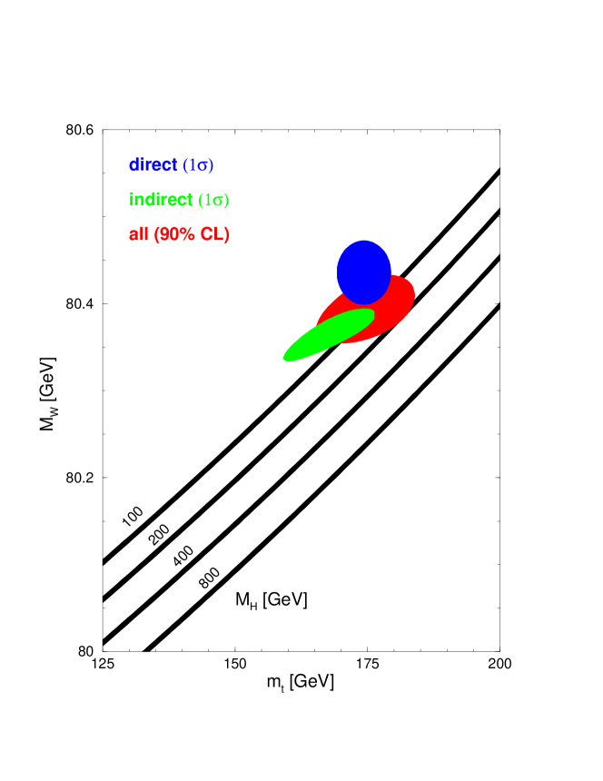
Figure 1: Allowed regions in $M_{W}$ vs $m_{t}$ from direct, indirect, and combined data, compared with the standard model expectations as a function of $M_{H}$. From [7].

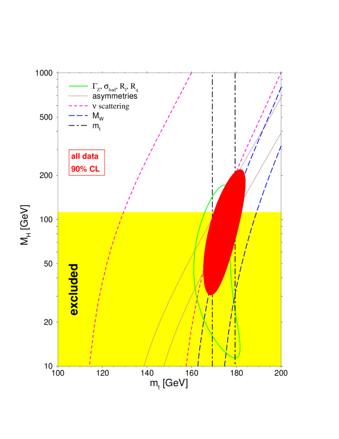
Figure 2: Allowed regions in $M_{H}$  vs $m_{t}$ from precision data, compared with the direct exclusion limits from LEP 2. From [7].

Figure 3: Probability density for $M_{H}$, including direct LEP 2 data and indirect constraints. From [17].

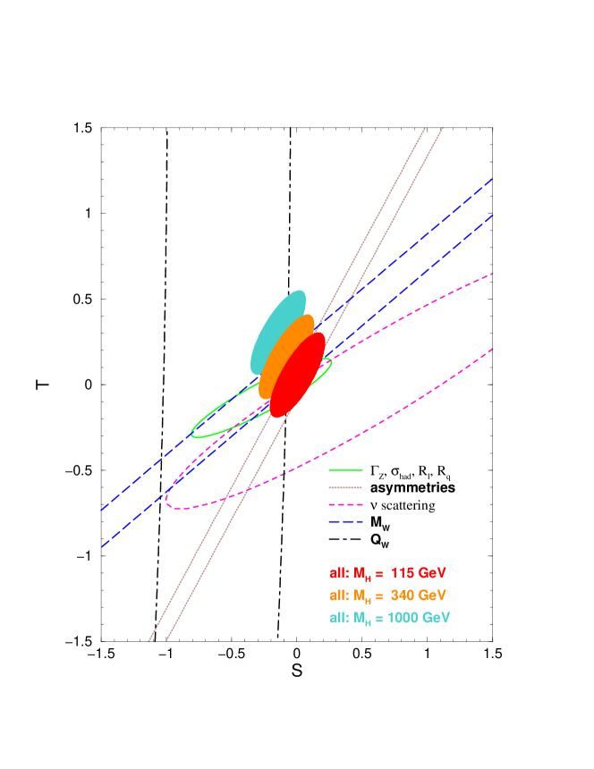
Figure 4: Allowed regions in $S$ vs $T$. From [7].

Figure 5: Predicted values of $S$ and $T$ for three models of supersymmetry breaking, compared with the experimentally allowed regions. Updated from [22].

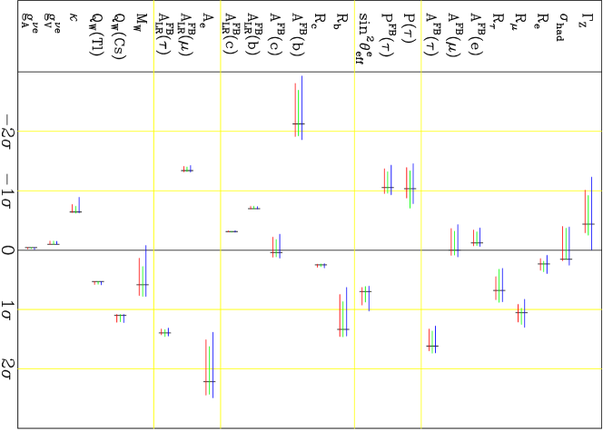
Figure 6: Changes in pulls of observables in three models of supersymmetry breaking, compared with the standard model. Updated from [22].

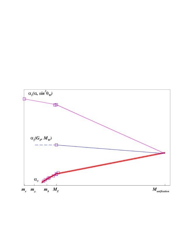
Figure 7: Running inverse gauge couplings in the MSSM. Experimental values at low energies are also shown. From [23].

References

- [1] For complete references, see J. Erler and P. Langacker, Electroweak Model and Constraints on New Physics, in Review of Particle Physics, D. E. Groom et al., Eur. Phys. J. C15, 1 (2000); Precision Tests of the Standard Electroweak Model, ed. P. Langacker (Singapore, World, 1995); P. Langacker, M. Luo and A. K. Mann, Rev. Mod. Phys. 64, 87 (1992).
- [2] J. E. Kim et al., Rev. Mod. Phys. 53, 211 (1981).
- [3] U. Amaldi et al., Phys. Rev. D 36, 1385 (1987).
- [4] G. Costa et al., Nucl. Phys. B297, 244 (1988).
- [5] P. Langacker, Comments Nucl. Part. Phys. 19, 1 (1989).
- [6] W. Marciano, these proceedings.
- [7] Updated from [1].
- [8] LEP Collaborations, hep-ex/0101027. Figures and other materials are available at http://www.cern.ch/LEPEWWG/.
- [9] D. Bardin, these proceedings.
- [10] W. Hollik, these proceedings.
- [11] G. Passarino, these proceedings.
- [12] T. Kinoshita, these proceedings.
- [13] F. Jegerlehner, these proceedings.
- [14] J. Erler, S. Heinemeyer, W. Hollik, G. Weiglein and P. M. Zerwas, Phys. Lett. B486, 125 (2000).
- [15] J. Erler, hep-ph/0005084. GAPP, as well as fit results, are available at www.physics.upenn.edu/erler/electroweak/
- [16] J. Erler, Phys. Rev. D59, 054008 (1999).
- [17] J. Erler, hep-ph/0010153 and these proceedings.
- [18] G. Degrassi, these proceedings.
- [19] A. Gurtu, Precision Tests of the Electroweak Gauge Theory, ICHEP 2000, Osaka, August 2000.
- [20] S. Eidelman and F. Jegerlehner, Z. Phys. C67, 585 (1995).
- [21] B. Pietrzyk, The Global Fit to Electroweak Data, ICHEP 2000.
- [22] J. Erler and D. M. Pierce, Nucl. Phys. B526, 53 (1998).
- [23] P. Langacker and N. Polonsky, Phys. Rev. D 52, 3081 (1995).
- [24] This work was supported by the U.S. Department of Energy grant DOE-EY-76-02-3071