Infrared Divergence and Twist-3 Distribution Amplitudes in QCD Factorization For $B\rightarrow PP$

Abstract

Since b quark mass is not asymptotically large, chirally enhanced corrections which arise from twist-3 wave functions may be important in B decays. We thus evaluate the hadronic matrix elements with the final light pseudoscalar mesons described by leading twist and twist-3 distribution amplitudes. We find that chirally enhanced corrections can be included consistently in the framework of QCD factorization only if the twist-3 distribution amplitudes are symmetric. We then give explicit expressions of $a_{i}^{p}$ for $B\rightarrow\pi\pi$ at the next-to-leading order of $\alpha_{s}$ including chirally enhanced corrections. We also briefly discuss the divergence appeared in the hard spectator contributions.

PACS numbers 13.25.Hw 12.38.Bx

Non-leptonic two-body B decays are crucial for us to extract CKM matrix elements and uncover the origin of CP violations. Experimentally, with the running of B factories, there will accumulate a great amount of data on various B decay channels. Theoretically, however, how to extract CKM matrix elements from non-leptonic B rare decays with model-independence is still an open question due to the complexity of strong interaction. In the following, we first give a theoretical sketch on non-leptonic B decays.

It is well known that the amplitude for the decay $B\rightarrow P_{1}P_{2}$ can be expressed as [1]:

$${\cal A}(B\rightarrow P_{1}P_{2})\propto\sum_{i}\lambda_{i}C_{i}(\mu)\langle P_{1}P_{2}|Q_{i}(\mu)|B\rangle,$$ (1)

where $\lambda_{i}$ is a CKM factor, $C_{i}(\mu)$ is a Wilson coefficient which incorporates short distance contributions from strong interactions and therefore is computable by making use of operator product expansion and renormalization group equations, $\langle P_{1}P_{2}|Q_{i}(\mu)|B\rangle$ is a hadronic matrix element. Obviously, if we want to extract CKM factor from B decays, the hadronic matrix elements should be evaluated reliably. However, due to our ignorance on hadronization, it would be a great challenge to calculate these hadronic matrix elements reliably from first principles. A commonly used approximation is naive factorization assumption, which is based on Bjorken’s color transparency argument [2]: b quark decays and transfers a large momentum to final light quarks, in which two fast-moving, nearly collinear final quarks with appropriate color can be viewed as a small color dipole which will not significantly interact with the soft gluons and finally form an emitted meson. Then we have:

$$\langle P_{1}P_{2}|Q_{i}(\mu)|B\rangle=\langle P_{1}|J_{1}|0\rangle\langle P_{2}|J_{2}|B\rangle,$$ (2)

where $P_{1}$ labels the emitted meson and $P_{2}$ labels another light meson which absorbs the spectator quark from B meson. This approximation completely ignores non-factorizable contributions which connect the emitted meson to the spectator system and expresses the hadronic matrix elements in terms of meson decay constants and form factors. Since decay constants and form factors can be, at least in principle, well determined from other experiments, the branching ratios of non-leptonic B decays are obtained under this assumption. The main deficiency of this approximation is that non-factorizable contributions are completely missing. In consequence, the hadronic matrix elements lose their scheme- and scale-dependence. Noting that Wilson coefficients are scheme- and scale-dependent, the corresponding decay width will also depend on renormalization scheme and scale which is unphysical. This is a clear indication that non-factorizable contributions, which amount to final-state rescattering and strong interaction phase shift, are important. Several generalizations of naive factorization assumption have been proposed to phenomenologically parameterize non-factorizable contributions. Since this kind of parameterization has no relation to, and therefore does not gain any information from, the underlying QCD dynamics, the resulting predictions on B decays are still model-dependent.

In ref [3, 4], Beneke, Buchalla, Neubert and Sachrajda proposed a promising QCD factorization method: The hadronic matrix elements $\langle P_{1}P_{2}|Q_{i}(\mu)|B\rangle$ contain two distinct scale: one is a large scale $\mu={\cal O}(m_{b})$, the other is $\Lambda_{QCD}$ which is the scale of hadronization. In the heavy quark limit, they show that the short distance contributions which are related to the large scale $\mu={\cal O}(m_{b})$ can be, at least at one-loop order, separated from the long distance effects and are thus calculable. Furthermore, the long distance effects can be parameterized by light-cone distribution amplitudes and non-perturbative form factors. Thus, the factorization formula can be explicitly expressed as: [3, 4]

$$\langle P_{1}P_{2}|Q_{i}|B\rangle=F^{B\rightarrow P_{2}}(0)\int\limits_{0}^{1}dxT^{I}_{i}(x)\Phi_{P_{1}}(x)+\int\limits_{0}^{1}d\xi dxdyT_{i}^{II}(\xi,x,y)\Phi_{B}(\xi)\Phi_{P_{1}}(x)\Phi_{P_{2}}(y),$$ (3)

where $\Phi_{B}(\xi)$ and $\Phi_{P_{i}}(x)$ are the leading-twist light-cone distribution amplitudes of B and the final light mesons respectively, $T^{I,II}_{i}$ denote hard-scattering kernels which are calculable order by order in perturbative theory. This formula holds for the case that the emitted meson $P_{1}$ is a light meson [3, 7, 8] or an onia of two heavy quarks [4, 9, 10] no matter whether $P_{2}$ is a heavy or light meson. But in this article we will focus on the case that B decays to two light pseudoscalar mesons.

In ref [3, 4], the authors pointed out that the equality sign of eq. (3) is valid only in the heavy quark limit. So if the heavy quark limit is an adequate approximation for B meson, or in another word, if power corrections in $1/m_{b}$ can be safely neglected, then everything is perfect. At the zero order of $\alpha_{s}$, it can reproduce ”naive factorization”, at the higher order of $\alpha_{s}$, the corrections can be systematically calculated in Perturbative QCD which will restore the scheme- and scale- dependence for the hadronic matrix elements. Therefore, the decay amplitudes of B meson can be reliably evaluated from first principles, and the necessary inputs are heavy-to-light form factors and light-cone distribution amplitudes. But in the real world, bottom quark mass is not asymptotically large(but about $4.8~{}GeV$), therefore it may be necessary to consider power corrections in $1/m_{b}$. Unfortunately there are a variety of sources which may contribute to power corrections in $1/m_{b}$, examples are higher twist distribution amplitudes, hard spectator interaction and transverse momenta of quarks in the light meson. Furthermore, there is no known systematic way to evaluate these power corrections for exclusive decays. Though naively, it is expected that power corrections may be neglected because $\Lambda_{QCD}/m_{b}\simeq 1/15$ is a small number, power suppression may numerically fail in some cases. An obvious and possibly the most important case is chirally enhanced power corrections. As pointed out in ref [3], numerically the enhanced factor $r_{\chi}=\frac{2m_{\pi}^{2}}{m_{b}(m_{u}+m_{d})}\simeq 1.18$ which makes the power suppression completely fail. This parameter is multiplied by $a_{6}$ and $a_{8}$, where $a_{6}$ is very important numerically in penguin-dominated B decays. So an evaluation of the hadronic matrix elements including chirally enhanced corrections may be phenomenologically or numerically important. In the following, we will examine this problem in some details.

Chirally enhanced corrections arise from twist-3 light-cone distribution amplitudes, generally called $\Phi_{p}(x)$ and $\Phi_{\sigma}(x)$. For light pseudoscalar mesons, they are defined as [5]

$$\langle P(p^{\prime})|{\bar{q}}(y){\it i}\gamma_{5}q(x)|0\rangle = f_{P}\mu_{P}\int_{0}^{1}{\it du~{}e}^{i(up^{\prime}\cdot y+{\bar{u}}p^{\prime}\cdot x)}\Phi_{p}(u),$$ (4)

$$\langle P(p^{\prime})|{\bar{q}}(y)\sigma_{\mu\nu}\gamma_{5}q(x)|0\rangle = if_{P}\mu_{P}(p^{\prime}_{\mu}z_{\nu}-p^{\prime}_{\nu}z_{\mu})\int_{0}^{1}{\it du~{}e}^{i(up^{\prime}\cdot y+\bar{u}p^{\prime}\cdot x)}\frac{\Phi_{\sigma}(u)}{6},$$ (5)

where $\mu_{p}=\frac{M^{2}_{p}}{m_{1}+m_{2}}$, $z=y-x$, $m_{1}$ and $m_{2}$ are the corresponding current quark masses. If we want to generalize QCD factorization method to include chirally enhanced corrections consistently, we should describe the emitted light meson with leading twist-2 and twist-3 distribution amplitudes [6]:

$$\langle P(p^{\prime})|{\bar{q}_{\alpha}}(y)q_{\delta}(x)|0\rangle = \frac{if_{P}}{4}\int_{0}^{1}{\it du~{}e}^{i(up^{\prime}\cdot y+{\bar{u}}p^{\prime}\cdot x)}$$ (6)

$$\times \left\{/{\hskip-7.11317pt}p^{\prime}\gamma_{5}\Phi(u)-\mu_{P}\gamma_{5}\left(\Phi_{p}(u)-\sigma_{\mu\nu}p^{\prime\mu}z^{\nu}\frac{\Phi_{\sigma}(u)}{6}\right)\right\}_{\delta\alpha}.$$ (7)

A technical proof of factorization requires that the hard scattering kernels in Eq.(3) are infrared finite. Authors of Ref [3, 4] have shown it explicitly with leading twist distribution amplitudes. Then a basic and perhaps a difficult task for us is to show the infrared finiteness of the hard-scattering kernels using twist-3 distribution amplitudes after summing over the four vertex correction diagrams (Fig. 1(a)-(d)).

The start point for B decays is $|\Delta B|=1$ effective Hamiltonian [1]:

$${\cal{H}}_{eff} = \frac{G_{F}}{\sqrt{2}}\left[\sum_{q=u,c}v_{q}\left(C_{1}(\mu)Q^{q}_{1}(\mu)+C_{2}(\mu)Q^{q}_{2}(\mu)+\sum_{k=3}^{10}C_{k}(\mu)Q_{k}(\mu)\right)\right.$$ (9)

$$-\left.v_{t}(C_{7\gamma}Q_{7\gamma}+C_{8G}Q_{8G})\frac{}{}\right]+h.c.,$$

where $v_{q}=V_{qb}V_{qd}^{*}$(for $b\rightarrow d$ transition) or $v_{q}=V_{qb}V_{qs}^{*}$(for $b\rightarrow s$ transition) and $C_{i}(\mu)$ are Wilson coefficients which have been evaluated to next-to-leading order approximation. The four-quark operators $Q_{i}$ are

$$\begin{array}[]{l}\begin{array}[]{ll}Q^{u}_{1}=(\bar{u}_{\alpha}b_{\alpha})_{V-A}(\bar{q}_{\beta}u_{\beta})_{V-A}&Q^{c}_{1}=(\bar{c}_{\alpha}b_{\alpha})_{V-A}(\bar{q}_{\beta}c_{\beta})_{V-A}\\ Q^{u}_{2}=(\bar{u}_{\alpha}b_{\beta})_{V-A}(\bar{q}_{\beta}u_{\alpha})_{V-A}&Q^{c}_{2}=(\bar{c}_{\alpha}b_{\beta})_{V-A}(\bar{q}_{\beta}c_{\alpha})_{V-A}\\ Q_{3}=(\bar{q}_{\alpha}b_{\alpha})_{V-A}\sum\limits_{q^{\prime}}(\bar{q}^{{}^{\prime}}_{\beta}q^{{}^{\prime}}_{\beta})_{V-A}&Q_{4}=(\bar{q}_{\beta}b_{\alpha})_{V-A}\sum\limits_{q^{\prime}}(\bar{q}^{{}^{\prime}}_{\alpha}q^{{}^{\prime}}_{\beta})_{V-A}\\ Q_{5}=(\bar{q}_{\alpha}b_{\alpha})_{V-A}\sum\limits_{q^{\prime}}(\bar{q}^{{}^{\prime}}_{\beta}q^{{}^{\prime}}_{\beta})_{V+A}&Q_{6}=(\bar{q}_{\beta}b_{\alpha})_{V-A}\sum\limits_{q^{\prime}}(\bar{q}^{{}^{\prime}}_{\alpha}q^{{}^{\prime}}_{\beta})_{V+A}\\ Q_{7}=\frac{3}{2}(\bar{q}_{\alpha}b_{\alpha})_{V-A}\sum\limits_{q^{\prime}}e_{q^{\prime}}(\bar{q}^{{}^{\prime}}_{\beta}q^{{}^{\prime}}_{\beta})_{V+A}&Q_{8}=\frac{3}{2}(\bar{q}_{\beta}b_{\alpha})_{V-A}\sum\limits_{q^{\prime}}e_{q^{\prime}}(\bar{q}^{{}^{\prime}}_{\alpha}q^{{}^{\prime}}_{\beta})_{V+A}\\ Q_{9}=\frac{3}{2}(\bar{q}_{\alpha}b_{\alpha})_{V-A}\sum\limits_{q^{\prime}}e_{q^{\prime}}(\bar{q}^{{}^{\prime}}_{\beta}q^{{}^{\prime}}_{\beta})_{V-A}&Q_{10}=\frac{3}{2}(\bar{q}_{\beta}b_{\alpha})_{V-A}\sum\limits_{q^{\prime}}e_{q^{\prime}}(\bar{q}^{{}^{\prime}}_{\alpha}q^{{}^{\prime}}_{\beta})_{V-A}\\ \end{array}\end{array}$$ (10)

and

$$Q_{7\gamma}=\frac{e}{8\pi^{2}}m_{b}\bar{q}_{\alpha}\sigma^{\mu\nu}(1+\gamma_{5})b_{\alpha}F_{\mu\nu},~{}~{}Q_{8G}=\frac{g}{8\pi^{2}}m_{b}\bar{q}_{\alpha}\sigma^{\mu\nu}t^{a}_{\alpha\beta}b_{\beta}G^{a}_{\mu\nu},~{}~{}(q=d~{}{\rm or}~{}s).$$ (11)

With these effective operators, $B\rightarrow P_{1}P_{2}$ decay amplitudes in QCD factorization can be written as:

$$A(B\rightarrow P_{1}P_{2})=\frac{G_{F}}{\sqrt{2}}\sum\limits_{p=u,c}\sum\limits_{i=1,10}v_{p}a^{p}_{i}\langle P_{1}P_{2}|Q_{i}|B\rangle_{F},$$ (12)

where $v_{p}$ is CKM factor, $\langle P_{1}P_{2}|Q_{i}|B\rangle_{F}$ is the factorized matrix element. We will calculate QCD coefficients $a_{i}^{p}$ and show explicitly that they are infrared finite.

Infrared divergences exist in vertex correction diagrams (Fig.1(a)-(d)), so let us first consider these diagrams. For $(V-A)\bigotimes(V-A)$ and $(S+P)\bigotimes(S-P)$ operators, twist-3 distribution amplitudes make no contribution because of their Lorentz structures. Therefore, QCD coefficients $a_{i}^{p}$ (except for $a_{6}^{p}$ and $a_{8}^{p}$) are nearly as same as those obtained in Ref [3, 7, 8] where leading twist distribution amplitudes are considered. The only difference is hard-spectator term (Fig.1(g)-(h)) which have been shown in Ref [11, 12], we will discuss it later. As to $(V+A)\bigotimes(V-A)$ operator, there are some subtleties in regularizing the infrared divergences. If we use dimension regularization, the infrared finiteness will not hold after summing over those four vertex correction diagrams. That is because wave functions are defined in 4-dimensions, it may be unconsistent to naively extend its usage to d-dimensions. Thus we assign a virtual mass to the gluon propagator and regularize the infrared integrals in four dimensions. For the twist-3 distribution amplitudes $\Phi_{p}(x)$, the calculations are performed in momentum space. Then it is straightforward to verify that the vertex correction contributions of $(V+A)\bigotimes(V-A)$ operator to $(S+P)\bigotimes(S-P)$ are infrared finite:

$$V=-\frac{\alpha_{s}}{4\pi}\frac{C_{F}}{N}\int_{0}^{1}dx\Phi_{p}(x)\{i\pi\log\frac{x}{\bar{x}}+\log\frac{x}{\bar{x}}-Li_{2}(-\frac{\bar{x}}{x})+Li_{2}(-\frac{x}{\bar{x}})+6\},$$ (13)

where $\bar{x}=1-x$ and $Li_{2}(x)$ is dilogarithm function. On the other hand, when considering $\Phi_{\sigma}$, we have to do the calculations in coordinate space according to Eq.(5). For example, let us consider Fig. 2. In coordinate space, we have:

$${\cal A} = \int d^{4}x_{1}d^{4}x_{2}d^{4}x_{3}~{}{\bar{u}_{\rho}}e^{iq^{\prime}\cdot x_{3}}~{}\gamma_{\lambda}(1+\gamma_{5})\int\frac{d^{4}k_{2}}{(2\pi)^{4}}\frac{i/{\hskip-7.11317pt}k_{2}}{k_{2}^{2}}e^{-ik_{2}\cdot(x_{3}-x_{2})}~{}[-ig_{s}\gamma^{\alpha}(T^{a})_{\rho\sigma}]$$ (16)

$$\frac{if_{P}\mu_{P}}{4N_{c}}\sigma_{\mu\nu}\gamma_{5}q^{\mu}(x_{3}-x_{2})^{\nu}\int dve^{i(vq\cdot x_{3}+{\bar{v}}q\cdot x_{2})}\frac{\Phi_{\sigma}(v)}{6}\delta_{\beta\sigma}~{}\gamma^{\lambda}(1-\gamma_{5})$$

$$\int\frac{d^{4}k_{1}}{(2\pi)^{4}}\frac{i(/{\hskip-7.11317pt}k_{1}+m_{b})}{k_{1}^{2}-m_{b}^{2}}e^{-ik_{1}\cdot(x_{3}-x_{1})}~{}[-ig_{s}\gamma_{\alpha}(T^{a})_{\beta\alpha}]~{}e^{-ip\cdot x_{1}}b_{\alpha}~{}\int\frac{d^{4}k}{(2\pi)^{4}}\frac{-i}{k^{2}-m_{g}^{2}}e^{-ik\cdot(x_{2}-x_{1})}$$

$$= \int dvd^{4}x_{1}d^{4}x_{2}d^{4}x_{3}\frac{d^{4}k}{(2\pi)^{4}}\frac{d^{4}k_{1}}{(2\pi)^{4}}\frac{d^{4}k_{2}}{(2\pi)^{4}}~{}{\bar{u}_{\rho}}e^{iq^{\prime}\cdot x_{3}}~{}e^{-ik_{2}\cdot(x_{3}-x_{2})}$$ (18)

$$\frac{if_{P}\mu_{P}}{4N_{c}}q^{\mu}(x_{3}-x_{2})^{\nu}\frac{\Phi_{\sigma}(v)}{6}\delta_{\beta\sigma}e^{i(vq\cdot x_{3}+{\bar{v}}q\cdot x_{2})}~{}e^{-ik_{1}\cdot(x_{3}-x_{1})}~{}e^{-ik\cdot(x_{2}-x_{1})}~{}e^{-ip\cdot x_{1}}b_{\alpha}\cdot H_{\mu\nu}(k,k_{1},k_{2})$$

$$= \left.(2\pi)^{4}\delta^{4}(p-q-q^{\prime})~{}\frac{f_{P}\mu_{P}}{4N_{c}}\int dv\frac{\Phi_{\sigma}(v)}{6}\int\frac{d^{4}k}{(2\pi)^{4}}~{}{\bar{u}_{\rho}}q^{\mu}\frac{\partial}{\partial k_{2\nu}}H_{\mu\nu}(k,p-k,k_{2})\right|_{k_{2}=k-{\bar{v}}q}~{}b_{\alpha},$$ (19)

where $H_{\mu\nu}(k,k_{1},k_{2})$ contains the Lorentz structure and propagators of the hard scattering kernels:

$$H_{\mu\nu}(k,k_{1},k_{2}) = \gamma_{\lambda}(1+\gamma_{5})~{}\frac{i/{\hskip-7.11317pt}k_{2}}{k_{2}^{2}}[-ig_{s}\gamma^{\alpha}(T^{a})_{\rho\sigma}]~{}\sigma_{\mu\nu}\gamma_{5}~{}\gamma^{\lambda}(1-\gamma_{5})$$ (21)

$$\frac{i(/{\hskip-7.11317pt}k_{1}+m_{b})}{k_{1}^{2}-m_{b}^{2}}~{}[-ig_{s}\gamma_{\alpha}(T^{a})_{\beta\alpha}]~{}\frac{-i}{k^{2}-m_{g}^{2}}\delta_{\beta\sigma}.$$

After a lengthy derivation, we can regularize the infrared divergences with a gluon virtual mass $m_{g}$:

$${\rm Fig.1(a)} \sim -\frac{\alpha_{s}}{4\pi}\frac{C_{F}}{N_{c}}\frac{\Phi_{\sigma}(v)}{v}\{\frac{\log^{2}\mu}{2}+2\log(-v)\log\mu-4\log v\log\mu+\log\mu+{\rm finite~{}terms}\}~{},$$ (22)

$${\rm Fig.1(b)} \sim \frac{\alpha_{s}}{4\pi}\frac{C_{F}}{N_{c}}\frac{\Phi_{\sigma}(v)}{\bar{v}}\{\frac{\log^{2}\mu}{2}+2\log(-{\bar{v}})\log\mu-4\log{\bar{v}}\log\mu+\log\mu+{\rm finite~{}terms}\}~{},$$ (23)

$${\rm Fig.1(c)} \sim \frac{\alpha_{s}}{4\pi}\frac{C_{F}}{N_{c}}\frac{\Phi_{\sigma}(v)}{v}\{\log^{2}\mu-2\log(-v)\log\mu+3\log\mu+{\rm finite~{}terms}\}~{}.$$ (24)

$${\rm Fig.1(d)} \sim -\frac{\alpha_{s}}{4\pi}\frac{C_{F}}{N_{c}}\frac{\Phi_{\sigma}(v)}{\bar{v}}\{\log^{2}\mu-2\log(-{\bar{v}})\log\mu+3\log\mu+{\rm finite~{}terms}\}~{},$$ (25)

where $\mu=m_{g}^{2}/m_{b}^{2}$. From the above equations, it is observed that, in the case of $\Phi_{\sigma}$ distribution amplitudes, the terms with infrared divergence in vertex correction diagrams can not cancel unless $\Phi_{\sigma}(v)$ is a symmetric function: $\Phi_{\sigma}(v)=\Phi_{\sigma}(\bar{v})$. This is an unexpected result, which means QCD factorization is violated for asymmetric twist-3 light-cone distribution amplitudes. This indicates that chirally enhanced corrections can be included consistently in the framework of QCD factorization only when twist-3 light-cone distribution amplitudes are symmetric. Therefore, in the following, we will implicitly assume a symmetric twist-3 light-cone distribution amplitude for light pseudoscalar mesons. It is then straightforward to show that vertex corrections of $(V+A)\otimes(V-A)$ operator are completely canceled after summing over four diagrams in the case of $\Phi_{\sigma}$ distribution amplitude.

For penguin contractions (Fig.1(e)-(f)) and hard spectator diagrams (Fig.1(g)-(h)), we shall also do the calculations in coordinate space when $\Phi_{\sigma}(v)$ is included. When treating penguin contractions, it should be careful that Fig.1(e) contains two kinds of topology, which is displayed in Fig.3. They are equivalent in 4 dimensions according to Fierz relations. However, since penguin corrections contain ultraviolet divergences, we must do calculations in d dimensions where these two kinds of topology are not equivalent [13]. We did not notice it and therefore obtained a wrong term $-\frac{2f}{3}C_{4}$ in the expression of $a_{4}^{p}$ in [7]. We also obtained a wrong term $(C3+C4/N)/3$ and missed a term of $(C4+C3/N)$ in the expression of $a_{10}^{p}$ in [7] for the same reason.

Then as an illustration, the explicit expressions of $a_{i}^{p}$ ($i=1$ to $10$) for $B\rightarrow\pi\pi$ (using symmetric light-cone distribution amplitudes of the pion) are obtained. But it is easy to generalize these formulas to the case that the final states are other light pseudoscalars. We now list $a_{i}^{p}$ for $B\rightarrow\pi\pi$ as follows:

$$a_{1}^{u} = C_{1}+\frac{C_{2}}{N}+\frac{\alpha_{s}}{4\pi}\frac{C_{F}}{N}C_{2}F,$$ (26)

$$a_{2}^{u} = C_{2}+\frac{C_{1}}{N}+\frac{\alpha_{s}}{4\pi}\frac{C_{F}}{N}C_{1}F,$$ (27)

$$a_{3} = C_{3}+\frac{C_{4}}{N}+\frac{\alpha_{s}}{4\pi}\frac{C_{F}}{N}C_{4}F,$$ (28)

$$a_{4}^{p} = C_{4}+\frac{C_{3}}{N}+\frac{\alpha_{s}}{4\pi}\frac{C_{F}}{N}C_{3}F$$ (31)

$$-\frac{\alpha_{s}}{4\pi}\frac{C_{F}}{N}\left\{C_{1}(\frac{4}{3}\log\frac{\mu}{m_{b}}+G(s_{p})-\frac{2}{3})+(C_{3}-\frac{C_{9}}{2})(\frac{8}{3}\log\frac{\mu}{m_{b}}+G(0)+G(1)-\frac{4}{3})\right.$$

$$+\sum_{q=u,d,s,c,b}(C_{4}+C_{6}+\frac{3}{2}{\rm e_{q}}C_{8}+\frac{3}{2}{\rm e_{q}}C_{10})\left.(\frac{4}{3}\log\frac{\mu}{m_{b}}+G(s_{q}))+G_{8}C_{8G}\right\},$$

$$a_{5} = C_{5}+\frac{C_{6}}{N}+\frac{\alpha_{s}}{4\pi}\frac{C_{F}}{N}C_{6}(-F-12),$$ (32)

$$a_{6}^{p} = C_{6}+\frac{C_{5}}{N}-\frac{\alpha_{s}}{4\pi}\frac{C_{F}}{N}6C_{5}$$ (37)

$$-\frac{\alpha_{s}}{4\pi}\frac{C_{F}}{N}\left\{C_{1}((1+\frac{2}{3}A_{\sigma})\log\frac{\mu}{m_{b}}-\frac{7}{12}-\frac{1}{2}A_{\sigma}+G^{\prime}(s_{p})+G^{\sigma}(s_{p}))\right.$$

$$+\sum_{q=d,b}(C_{3}-\frac{C_{9}}{2})((1+\frac{2}{3}A_{\sigma})\log\frac{\mu}{m_{b}}-\frac{7}{12}-\frac{1}{2}A_{\sigma}+G^{\prime}(s_{q})+G^{\sigma}(s_{q}))$$

$$+\sum_{q=u,d,s,c,b}(C_{4}+C_{6}+\frac{3}{2}{\rm e_{q}}C_{8}+\frac{3}{2}{\rm e_{q}}C_{10})\left((1+\frac{2}{3}A_{\sigma})\log\frac{\mu}{m_{b}}-\frac{1}{12}-\frac{1}{6}A_{\sigma}+G^{\prime}(s_{q})+G^{\sigma}(s_{q})\right)$$

$$\left.+(\frac{3}{2}+A_{\sigma})C_{8G}\right\},$$

$$a_{7} = C_{7}+\frac{C_{8}}{N}+\frac{\alpha_{s}}{4\pi}\frac{C_{F}}{N}C_{8}(-F-12),$$ (38)

$$a_{8}^{p} = C_{8}+\frac{C_{7}}{N}-\frac{\alpha_{s}}{4\pi}\frac{C_{F}}{N}6C_{7}$$ (43)

$$-\frac{\alpha_{em}}{9\pi}\left\{(C_{2}+\frac{C_{1}}{N})((1+\frac{2}{3}A_{\sigma})\log\frac{\mu}{m_{b}}-\frac{7}{12}-\frac{1}{2}A_{\sigma}+G^{\prime}(s_{p})+G^{\sigma}(s_{p}))\right.$$

$$+(C_{4}+\frac{C_{3}}{N})\sum_{q=d,b}\frac{3}{2}{\rm e_{q}}((1+\frac{2}{3}A_{\sigma})\log\frac{\mu}{m_{b}}-\frac{7}{12}-\frac{1}{2}A_{\sigma}+G^{\prime}(s_{q})+G^{\sigma}(s_{q}))$$

$$+(C_{3}+\frac{C_{4}}{N}+C_{5}+\frac{C_{6}}{N})\sum_{q=u,d,s,c,b}\frac{3}{2}{\rm e_{q}}\left((1+\frac{2}{3}A_{\sigma})\log\frac{\mu}{m_{b}}-\frac{1}{12}-\frac{1}{6}A_{\sigma}+G^{\prime}(s_{q})+G^{\sigma}(s_{q})\right)$$

$$\left.+(\frac{3}{4}+\frac{1}{2}A_{\sigma})C_{7\gamma}\right\},$$

$$a_{9} = C_{9}+\frac{C_{10}}{N}+\frac{\alpha_{s}}{4\pi}\frac{C_{F}}{N}C_{10}F,$$ (44)

$$a_{10}^{p} = C_{10}+\frac{C_{9}}{N}+\frac{\alpha_{s}}{4\pi}\frac{C_{F}}{N}C_{9}F-\frac{\alpha_{em}}{9\pi}\left\{(C_{2}+\frac{C_{1}}{N})(\frac{4}{3}\log\frac{\mu}{m_{b}}+G(s_{p})-\frac{2}{3})\right.$$ (47)

$$+(C_{4}+\frac{C_{3}}{N})\sum_{q=d,b}\frac{3}{2}{\rm e_{q}}(\frac{4}{3}\log\frac{\mu}{m_{b}}+G(s_{q})-\frac{2}{3})$$

$$+(C_{3}+\frac{C_{4}}{N}+C_{5}+\frac{C_{6}}{N})\sum_{q=u,d,s,c,b}\left.\frac{3}{2}{\rm e_{q}}(\frac{4}{3}\log\frac{\mu}{m_{b}}+G(s_{q}))+\frac{1}{2}G_{8}C_{7\gamma}\right\}.$$

Here $N=3$ is the number of color, $C_{F}=\frac{N^{2}-1}{2N}$ is the factor of color, $s_{q}=m_{q}^{2}/m_{b}^{2}$ and we define the other symbols in the above expressions as:

$$F=-12\ln\frac{\mu}{m_{b}}-18+f^{I}+f^{II},$$ (48)

$$f^{I}=\int\limits_{0}^{1}~{}dx~{}g(x)\Phi(x),~{}G_{8}=\int\limits_{0}^{1}~{}dx~{}G_{8}(x)\Phi(x),$$ (49)

$$G(s)=\int\limits_{0}^{1}~{}dx~{}G(s,x)\Phi(x),$$ (50)

$$G^{\prime}(s)=\int\limits_{0}^{1}~{}dx~{}G^{\prime}(s,x)\Phi_{p}(x),$$ (51)

$$G^{\sigma}(s)=\int\limits_{0}^{1}~{}dx~{}G^{\sigma}(s,x)\frac{\Phi_{\sigma}(x)}{6(1-x)},~{}~{}~{}~{}~{}A_{\sigma}=\int\limits_{0}^{1}~{}dx~{}\frac{\Phi_{\sigma}(x)}{6(1-x)},$$ (52)

here $\Phi(x)$($\Phi_{p}(x)$,$\Phi_{\sigma}(x)$) is leading twist (twist-3) wave function of the emitted pion, and the hard-scattering functions are

$$g(x)=3\frac{1-2x}{1-x}\ln x-3i\pi,~{}~{}G_{8}(x)=\frac{2}{1-x},$$ (53)

$$G(s,x)=-4\int\limits_{0}^{1}~{}du~{}u(1-u)\ln(s-u(1-u)(1-x)-i\epsilon),$$ (54)

$$G^{\prime}(s,x)=-3\int\limits_{0}^{1}~{}du~{}u(1-u)\ln(s-u(1-u)(1-x)-i\epsilon),$$ (55)

$$G^{\sigma}(s,x)=-2\int\limits_{0}^{1}~{}du~{}u(1-u)\ln(s-u(1-u)(1-x)-i\epsilon)$$ (56)

$$~{}~{}~{}~{}~{}~{}~{}~{}~{}~{}~{}~{}~{}~{}~{}+\int\limits_{0}^{1}~{}du~{}\frac{u^{2}(1-u)^{2}(1-x)}{s-u(1-u)(1-x)-i\epsilon}.$$ (57)

The contributions from the hard spectator scattering (Fig.1(g)-(h)) are reduced into the factor $f^{II}$. We take the wave function of B meson as $\gamma_{5}(/{\hskip-7.11317pt}P_{B}-M_{B})\Phi_{B}(\xi)$. Then an explicit calculations show that twist-3 distribution amplitudes of the emitted pion make no contributions to $f^{II}$. It means that there is no hard spectator contributions for $a_{6}^{p}$ and $a_{8}^{p}$. For other QCD coefficients $a_{i}^{p}$, we have:

$$f^{II}=\frac{4\pi^{2}}{N}\frac{f_{\pi}f_{B}}{F^{B\rightarrow\pi}_{+}(0)m_{B}^{2}}\int\limits_{0}^{1}~{}d\xi~{}\frac{\Phi_{B}(\xi)}{\xi}\int\limits_{0}^{1}~{}dx~{}\frac{\Phi(x)}{x}\int\limits_{0}^{1}~{}dy~{}\left[\frac{\Phi(y)}{1-y}+\frac{2\mu_{\pi}}{M_{B}}\frac{\Phi_{\sigma}(y)}{6(1-y)^{2}}\right].$$ (58)

Here $\Phi(x)$ is leading twist distribution amplitude of the emitted pion, $\Phi(y)$($\Phi_{\sigma}(y)$) is twist-2(twist-3) distribution amplitudes of the recoiled pion. This formula is consistent with the result of Ref. [9].

In the above expressions of $a_{i}^{p}$, $a_{6}^{p}$ and $a_{8}^{p}$ can now be evaluated to next-to-leading order of $\alpha_{s}$, which significantly reduce their scale-dependence. As to other QCD coefficients $a_{i}^{p}$, there contains a divergent integral in hard spectator term $f^{II}$. In the next paragraph, we will argue that this disturbing divergence may need further consideration. Here we simply assume that $\int\frac{dy}{y}\sim ln\frac{m_{b}}{\Lambda_{QCD}}$ (similar to what have been done in Ref [11, 12], though our assumption here is certainly an oversimplification). We thus illustrate numerically the scale-dependence of $a_{i}^{p}(\pi\pi)$ in Table.1. Here we use the asymptotic distribution amplitudes

$$\Phi(x)=\Phi_{\sigma}(x)=6x(1-x)~{}~{}{\rm and}~{}~{}\Phi_{p}(x)=1,$$ (59)

and the input parameters are taken as follows: $F^{B\pi}(0)=0.33$, $f_{B}=0.2~{}GeV$, $f_{\pi}=133~{}MeV$, the pole masses $m_{b}=4.8~{}GeV$, $m_{c}=1.4~{}GeV$, the $\overline{MS}$ masses ${\overline{m}_{t}}({\overline{m}_{t}})=170~{}GeV$, ${\overline{m}_{b}}({\overline{m}_{b}})=4.4~{}GeV$, $\overline{m}_{u}(2~{}GeV)=4.2~{}MeV$, $\overline{m}_{d}(2~{}GeV)=7.6~{}MeV$ and $\Lambda_{QCD}^{(5)}=225~{}MeV$.

We notice that the above approach of evaluating hard spectator contribution is naive. For instance, the scale of hard spectator contribution should be different from the vertex correction contribution. While it seems reasonable to take the scale $\mu\sim{\cal O}(m_{b})$ for the vertex correction diagrams to avoid large logarithm $\alpha_{s}\log\frac{\mu}{m_{b}}$, a natural choice of the scale of hard spectator contribution may be around ${\cal O}(1~{}GeV)$ because the average momentum squared of the exchanged gluon is about $1~{}GeV^{2}$. Another disturbing feature of hard spectator contribution is that, as pointed out in ref [11, 12], when including the contribution of $\Phi_{\sigma}$, there would appear divergent integral $\int_{0}^{1}dy\frac{1}{y}$ even if the symmetric distribution amplitude is applied. This divergent integral implies that the dominant contribution comes from the end-point region, or in another word, it is dominated by soft gluon exchange. However the transverse momentum may not be omitted in the end-point region [14], if so, the corresponding divergent integral would then changed to:

$$\int dy\frac{1}{y}\rightarrow\int dyd^{2}k_{T}\frac{\Psi(y,k_{T})}{y\xi m_{b}^{2}+k^{2}_{T}}.$$ (60)

As an illustration, we do not consider the $k_{T}$ dependence of wave functions (though it is certainly not a good approximation), then the above integral is proportional to:

$$\int\frac{dydk^{2}_{T}}{y\xi m_{b}^{2}+k^{2}_{T}}\propto\int\frac{dxdy}{x+y}.$$ (61)

The above integration converges now, furthermore it is not dominated by end-point contribution. This illustrates that the treatment of hard spectator diagrams may need further discussions.

There exists ”annihilation” contributions which may belong to chirally enhanced corrections. In Ref. [12], the authors have discussed this topic and find that a divergent integral $(\int\frac{dx}{x})^{2}$ will appear. We suspect that this divergence may disappear, similar to the hard spectator term, if the effect of transverse momenta can be included. It is also possible that ”annihilation” contributions are really dominated by soft interactions and thus violate factorization. Due to its complexity, we do not include ”annihilation” contributions in the expressions of $a_{i}^{p}$.

In summary, to generalize QCD factorization method to include chirally enhanced corrections consistently, the final light mesons should be described with leading twist and twist-3 distribution amplitudes. We demonstrate that the infrared finiteness of the hard scattering kernels can be obtained only if the twist-3 distribution amplitudes are symmetric. We then give explicit expressions of $a_{i}^{p}$ at next-to-leading order of $\alpha_{s}$ including chirally enhanced corrections. We also discuss briefly the disturbing hard spectator contributions.

QCD	$\mu=5.0~{}GeV$		$\mu=2.5~{}GeV$
Coefficients	NLO	LO	NLO	LO
$a_{1}^{u}$	$1.024+0.012i$	$1.017$	$1.034+0.024i$	$1.037$
$a_{2}^{u}$	$0.144-0.076i$	$0.188$	$0.123-0.100i$	$0.109$
$a_{3}$	$0.003+0.002i$	$0.002$	$0.004+0.004i$	$0.004$
$a_{4}^{u}$	$-0.027-0.014i$	$-0.029$	$-0.029-0.017i$	$-0.040$
$a_{4}^{c}$	$-0.033-0.007i$	$-0.029$	$-0.036-0.007i$	$-0.040$
$a_{5}$	$-0.003-0.003i$	$-0.005$	$-0.002-0.005i$	$-0.010$
$r_{\chi}a_{6}^{u}$	$-0.036-0.012i$	$-0.033$	$-0.037-0.011i$	$-0.040$
$r_{\chi}a_{6}^{c}$	$-0.039-0.005i$	$-0.033$	$-0.040-0.004i$	$-0.040$
$a_{7}\times 10^{5}$	$11.9+2.8i$	$13.8$	$0.0+5.4i$	$7.6$
$r_{\chi}a_{8}^{u}\times 10^{5}$	$36.8-10.9i$	$36.8$	$45.0-5.2i$	$39.8$
$r_{\chi}a_{8}^{c}\times 10^{5}$	$35.0-6.2i$	$36.8$	$44.2+3.1i$	$39.8$
$a_{9}\times 10^{5}$	$-936.1-13.4i$	$-928.4$	$-953.9-24.5i$	$-957.3$
$a_{10}^{u}\times 10^{5}$	$-81.8+58.8i$	$-141.4$	$-58.3+86.1i$	$-74.0$
$a_{10}^{c}\times 10^{5}$	$-85.2+63.5i$	$-141.4$	$-60.3+88.8i$	$-74.0$

TABLE I.: The QCD coefficients $a_{i}^{p}(\pi\pi)$ at NLO and LO for the renormalization scales at $\mu=5~{}GeV$ and $\mu=2.5~{}GeV$, where $r_{\chi}=\frac{2m_{\pi}^{2}}{m_{b}(m_{u}+m_{d})}$

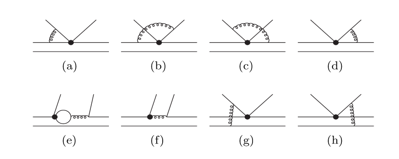
FIG. 1.: Order of $\alpha_{s}$ corrections to hard-scattering kernels. The upward quark lines represent the ejected quark pairs from b quark weak decays.

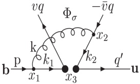
FIG. 2.:

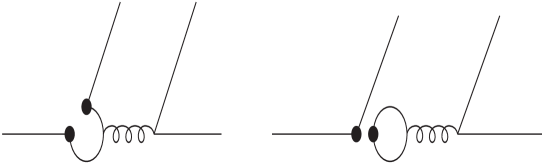
FIG. 3.: Two kinds of topology for penguin contractions.

REFERENCES

[1]
G. Buchalla, A.J. Buras and M.E. Lautenbacher, Rev. Mod. Phys.
, 1125 (1996).