EXTRAPOLATION OF $K\rightarrow\pi\pi$ DECAY AMPLITUDE

Abstract

We examine the uncertainties involved in the off-mass-shell extrapolation of the $K\rightarrow\pi\pi$ decay amplitude with emphasis on those aspects that have so far been overlooked or ignored. Among them are initial-state interactions, choice of the extrapolated kaon field, and the relation between the asymptotic behavior and the zeros of the decay amplitude. In the inelastic region the phase of the decay amplitude cannot be determined by strong interaction alone and even its asymptotic value cannot be deduced from experiment. More a fundamental issue is intrinsic nonuniqueness of off-shell values of hadronic matrix elements in general. Though we are hampered with complexity of intermediate-energy meson interactions, we attempt to obtain a quantitative idea of the uncertainties due to the inelastic region and find that they can be much larger than more optimistic views portray. If large uncertainties exist, they have unfortunate implications in numerical accuracy of computation of the direct CP violation parameter $\epsilon^{\prime}$.

I Introduction

Accurate computation of the long-distance QCD corrections for the decay $K\rightarrow\pi\pi$ is important in testing the underlying mechanism of CP violation with the $\epsilon^{\prime}$ parameter. When one obtains a real amplitude for $K\rightarrow\pi\pi$ by any method of calculation, its validity is limited to the unphysical region below $\pi\pi$ rescattering. On the kaon mass shell one must supply a phase by taking account of rescattering[1, 2]. However, rescattering affects a magnitude of amplitude in general. While the phase of amplitude arises solely from elastic rescattering in the case of $K\rightarrow\pi\pi$, the magnitude of amplitude is affected by inelastic scattering as well. Many attempts have been made to incorporate the final-state interaction (FSI) in the $K\rightarrow\pi\pi$ decay amplitudes, most recently by Palante and Pich[3] among others.

The final-state interaction (FSI) theory was first formulated in potential scattering in the 1950’s[4], then extended with dispersion relation to relativistic particle physics, often using the Omnès-Muskhelishvili (OM) representation[5]. When our interest was in very low energy phenomena, it was a good enough approximation to discard all but elastic FSI rescattering. In particle physics, however, inelastic rescattering can be potentially important to the magnitude of amplitude even when it does not contribute to the phase. If we knew the values of the phase at all energies, we could compute the magnitude with the OM representation apart from factors of zeros. However, the phase of a decay amplitude above the inelastic rescattering threshold has nothing to do with the inelastic scattering phase shift of strong interaction. It depends on decay operators even when all quantum numbers are the same.

In addition to inelastic rescattering, strong interactions take place in the initial state before $K$ decays. Though it does not contribute to the phase, the initial-state interaction (ISI) generates $p_{K}^{2}$ dependence for the off-shell amplitude just as the FSI does. The existing calculations of the FSI largely neglect the ISI effect. Once the inelastic FSI and the ISI are included, the OM representation is by no means ’universal” contrary to the statement often found in recent literature.

Extrapolation off mass shell involves a few more basic issues that have not been discussed. One is the asymptotic behavior of a decay amplitude far off mass shell, which is directly related to the number of zeros and the asymptotic phase $\delta(\infty)$ of the amplitude. In the elastic approximation, we may follow potential scattering theory and determine the asymptotic behavior by Levinson’s theorem[6]. In relativistic physics which contains inelasticity, Levinson’s theorem does not hold. Therefore we must determine in one way or another the value of $\delta(\infty)$ and the number of zeros and incorporate them in the OM representation.

Another issue is nonuniqueness of off-shell amplitudes, which is inherent in quantum field theory. According to a general theorem[7], on-shell amplitudes are unique no matter what operator one may choose for a particle field as long as it has a correct wave function renormalization and a right set of quantum numbers on mass shell. However, off-shell amplitudes can depend on choice of particle fields, which is by no means unique in the case of hadrons. In particular, the asymptotic behavior is sensitive to the choice. In order to write the OM representation uniquely, therefore, we must first define the kaon field and then determine the asymptotic behavior and the number of zeros of the decay amplitude.

Since we think that many of these basic issues in the off-shell extrapolation have been either improperly treated or entirely ignored in literature, we attempt to expose them and obtain some quantitative idea of the uncertainties associated with them in this paper. While a recent criticism[8] concerns mostly technical aspects of Ref.[3], we focus on more basic aspects of the FSI theory[9].

The paper is organized as follows: In Sec. II, we clarify distinction between the FSI and the ISI. For this purpose we write the $K\rightarrow\pi\pi$ amplitude first by the dispersion relation for scattering of a weak spurion off an on-shell kaon. In this dispersion relation, the FSI generates the $s$-channel singularities while the ISI contributes to the $u$-channel singularities. Then we write the OM representation by dispersing the kaon mass $p_{K}^{2}$ and show that both the FSI and the ISI contribute to the right-hand cuts in the OM representation. In Sec. III, we relate the number of zeros of amplitude to the asymptotic phase and magnitude in the OM representation in general. In Sec. IV, after reviewing the inherent ambiguity of an extrapolated particle field in field theory, we study the asymptotic behaviors of the $K\rightarrow\pi\pi$ amplitudes in QCD by defining the off-shell kaon field by the partially-conserved axial-vector current (PCAC) relation. In Sec. V, we interpolate the phases for the dominant $\Delta I=\frac{1}{2}$ amplitude and for the $\Delta I=\frac{3}{2}$ amplitude between the inelastic threshold and the high energy limit. Then we examine in detail the case that the decay amplitudes have the smallest number of zeros including the well-known low-energy zero. In this particular case we make quantitative discussion on the extrapolation effect by giving illustrative estimates of how much variation occurs in the extrapolation from $p_{K}^{2}=m_{\pi}^{2}$ to $m_{K}^{2}$. We find that the ISI and the inelastic FSI are not negligible even in the case of a single zero. In more general cases, uncertainty is larger. The source of the largest uncertainty is in the number of zeros and their locations.

II Dispersion relations

The decay matrix element for $K\rightarrow\pi\pi$ is written as

$$M=\langle\pi(p_{a})\pi(p_{b})^{out}|H_{W}(0)|K(p_{K})\rangle.$$ (1)

In actual computation an effective decay operator $c_{i}(\mu){\cal O}_{i}$ is chosen for $H_{W}$, which incorporates short-distance QCD effects in $c_{i}(\mu)$ by renormalization group. Since the interaction above the energy scale $\mu$ is included in $c_{i}(\mu){\cal O}_{i}$, we ought to truncate dispersion integrals accordingly, as we shall discuss later.

A Spurion scattering

Treat $H_{W}$ as the source of spurion $S$ by setting $\Box S=H_{W}$ and write a dispersion relation for the on-shell scattering,

$$S(p_{s})+K(p_{K})\rightarrow\pi(p_{a})+\pi(p_{b}),\;\;\;(p_{s}^{2}=0)$$ (2)

with the Mandelstam variables, $s=(p_{s}+p_{K})^{2}=(p_{a}+p_{b})^{2}$, $t=(p_{K}-p_{a})^{2}=(p_{s}-p_{b})^{2}$, and $u=(p_{K}-p_{b})^{2}=(p_{s}-p_{a})^{2}=m_{K}^{2}+2m_{\pi}^{2}-s-t$. The decay amplitude $M(s,t)$ at $t<(m_{K}+m_{\pi})^{2}$ is real analytic in the complex $s$-plane; $M(s^{*},t)=M(s,t)^{*}$. The right-hand cut starts at $s=4m_{\pi}^{2}$ while the left-hand cut starts at $u=(m_{K}+m_{\pi})^{2}$, namely, at $s=-2m_{K}m_{\pi}+m_{\pi}^{2}-t\;(\equiv s_{L})$. (See Fig. 1.) For $t$ fixed small, the $s\rightarrow\infty$ limit of $M(s,t)$ is determined by Regge asymptotic behavior of $K^{*}$ exchange. Since $\alpha_{K^{*}}(m_{\pi}^{2})\simeq 0.3$, one can write a once-subtracted dispersion relation in $s$ at the physical point $t=m_{\pi}^{2}$ as:

$$M(s,t)=M(s_{0},t)+\frac{s-s_{0}}{\pi}\int_{4m_{\pi}^{2}}^{\infty}\frac{{\rm Im}M(s^{\prime},t)}{(s^{\prime}-s)(s^{\prime}-s_{0})}ds^{\prime}+\frac{s-s_{0}}{\pi}\int_{-\infty}^{s_{L}}\frac{{\rm Im}M(s^{\prime},t)}{(s^{\prime}-s)(s^{\prime}-s_{0})}ds^{\prime}.$$ (3)

The decay amplitude is obtained by setting $p_{s}^{\mu}=0$, namely, $s=m_{K}^{2}$ and $t=u=m_{\pi}^{2}$. The first integral in Eq. (3) due to the $s$-channel intermediate states describes the FSI, both elastic and inelastic. Its discontinuity across the cut is given by

$${\rm Im}M(s,t)_{R}=\sum_{n}\pi(2\pi)^{3}\delta(p_{a}+p_{b}-p_{n})\langle\pi|j_{\pi}(0)|n^{out}\rangle\langle n^{out}|H_{w}(0)|K\rangle.$$ (4)

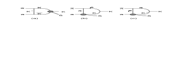
The lowest two-body inelastic intermediate state is $K\overline{K}$. The triangular diagram depicted in Fig. 2a is the simplest and probably the most important of the inelastic FSI. In contrast, the second integral of Eq. (3) arises from the $u$-channel intermediate states which give the discontinuity,

$${\rm Im}M(s,t)_{L}=-\sum_{n}\pi(2\pi)^{3}\delta(p_{K}-p_{b}-p_{n})\langle\pi|H_{W}(0)|n^{out}\rangle\langle n^{out}|j_{\pi}(0)|K\rangle.$$ (5)

The nearest left-hand singularity is generated by the process, $K\rightarrow\rho K\rightarrow\pi\pi$, namely, a virtual dissociation followed by a weak decay. (See Fig. 2b.) The diagram of Fig. 2b has no $s$-channel singularity and therefore cannot be identified with the FSI. Nonetheless, it contributes to the $s$ dependence of the amplitude. The process of the $K^{*}\pi$ intermediate state of Fig. 2c belongs to the same class. We call this class of diagrams as the ISI diagrams. Most generally, a single diagram can contribute to both the ISI and the FSI. It is clear from the two diagrams in Fig. 2 that the elastic and inelastic FSI alone, namely the $s$-channel singularities, are not sufficient to determine the $s$ dependence of $M(s)$. It is also obvious that the phase due to the diagrams of Fig. 2b and 2c are in no way related to scattering phase shifts of strong interaction at the corresponding energy.

B Phase representation

Having defined the ISI by the spurion dispersion relation, we now write the OM dispersion relation by taking the initial kaon off mass shell. If we follow the reduction formula[10], we would reduce one of the pions in addition to the kaon. Rather than handling product of three operators $j_{\pi}$, $j_{K}$, and $H_{W}$, we may take more an intuitive approach by relying on perturbative diagram analysis of analyticity[11].

Choosing a suitable extrapolation field for the kaon, we can write a dispersion relation in the variable $p_{K}^{2}$ keeping $p_{s}^{\mu}=0$. Since $s=(p_{K}+p_{s})^{2}=p_{K}^{2}$ for $p_{s}^{\mu}=0$, we denote $p_{K}^{2}$ by $s$. In terms of the Mandelstam variables previously defined, we fix $t$ and $u$ to $m_{\pi}^{2}$ keeping $s$ as the only variable. Then all singularities appear on the positive real axis of $s$. (See Fig. 3.) The intermediate states $K\overline{K}$, $\rho K$, and $K^{*}\pi$ of the diagrams in Fig. 2 generate cuts starting at $s=4m_{K}^{2}$, $(m_{\rho}+m_{K})^{2}$, and $(m_{K^{*}}+m_{\pi})^{2}$, respectively. To obtain the phase dispersion relation of Omnès-Muskhelishvili[5], we write a dispersion relation for the logarithm of the decay amplitude $M(s)$. Keeping in mind that zeros of $M(s)$ are singularities of $\ln M(s)$, we obtain

$$M(s)=\prod_{i=1}^{N}\biggl{(}\frac{s-s_{i}}{s_{0}-s_{i}}\biggr{)}M(s_{0})\exp\biggl{(}\frac{s-s_{0}}{\pi}\int_{4m_{\pi}^{2}}^{\infty}\frac{\delta(s^{\prime})}{(s^{\prime}-s)(s^{\prime}-s_{0})}ds^{\prime}\biggr{)},$$ (6)

where $\delta(s)=\arg M(s)$. In writing the dispersion integral for $\delta(s)$ with only one subtraction, we make the mild assumption that $\delta(s)$ does not keep rising or falling indefinitely for large $s$. Though the absorptive parts of the ISI diagrams and the inelastic FSI diagrams both appear on the right-hand cuts of the OM representation, they describe physically different processes. When we calculate the on-shell decay amplitudes, we are incorporating part of the ISI effect through the $K\rightarrow\pi$ form factor. To our knowledge, however, nobody has included the ISI process in the OM representation.

III Zeros of decay amplitude

The large $s$ behavior of $M(s)$ in Eq. (6) is determined by the number of zeros and the asymptotic value of the phase $\delta(\infty)$. It is straightforward to find that, up to logarithmic factors,

$$\lim_{s\rightarrow\infty}M(s)\sim s^{N-\delta(\infty)/\pi},$$ (7)

where we have normalized as $\delta(4m_{\pi}^{2})=0$ at the threshold. Therefore, once we know the large $s$ behavior of $|M(s)|$, the number of zeros is determined by $\delta(\infty)$. In potential theory, $M(s)$ is proportional to the inverse Jost function $1/f_{+}(k)$[4]. The Jost function $f_{+}(k)$[12] is analytic in the upper half plane of the complex variable $k(=(s/4-m_{\pi}^{2})^{1/2})$ and approaches unity at $|k|=\infty$. The zeros of $f_{+}(k)$ mean bound states. If we repeat the argument leading to Eq. (7) for $f_{+}(k)$ and use $\arg f_{+}(k)=-\delta(k)$ and $f_{+}(\infty)=1$, Levinson’s theorem[6] results; $N_{b}+\frac{1}{\pi}\delta(\infty)=0$, where $N_{b}$ is the number of zeros of $f_{+}(k)$, i.e., that of bound states. In potential theory, therefore, $\delta(\infty)=0$ in any channel that has no bound state. When inelastic scattering is included, however, $M(s)$ is no longer as simple as the inverse of the Jost function of potential scattering and therefore Levinson’s theorem does not hold.

It should be emphasized that above the inelastic threshold, the phase $\delta(s)$ of $M(s)$ has nothing to do with the phase shift of $\pi\pi\rightarrow\pi\pi$ scattering at the corresponding energy. The phase of $M(s)$ is a result of complicated interplay of strong and weak interactions unlike the scattering phase shift of strong interaction. (See Appendix A.) Therefore, it is nearly hopeless to determine $\delta(\infty)$ either experimentally or directly from theory. All we can hope is to determine $N-\delta(\infty)/\pi$, not $N$ and $\delta(\infty)$ separately, from the large $s$ behavior of $|M(s)|$ using Eq. (7).

We know that $M(s)$ has one zero in the low-energy region. In the flavor SU(3) symmetry limit of strong interaction with no electromagnetic or quark mass difference correction, charge-conjugation oddness of parity-violating $H_{W}$ requires that $K\rightarrow\pi\pi$ be forbidden in the $I=0$ channel[13]. Therefore, the $K\rightarrow\pi\pi$ decay amplitude vanishes at $p_{K}^{2}=p_{a}^{2}=p_{b}^{2}$ in this limit. It was shown in the soft-pion analysis of the 1960’s that the $\Delta I=\frac{1}{2}$ amplitude of $K\rightarrow\pi\pi$ vanishes like $\sim 2p_{K}^{2}-p_{a}^{2}-p_{b}^{2}$[14]. If SU(3) breaking enters only through the external meson momenta, therefore, $M(s)$ should vanish at $s=m_{\pi}^{2}$. This low-energy off-shell behavior is very robust for the $\Delta I=\frac{1}{2}$ amplitude. The $\Delta I=\frac{3}{2}$ decay through pure weak interaction (i.e., no electromagnetic or quark mass difference correction) shows the same behavior. However, we do not know how many more zeros $M(s)$ may have outside the soft-meson region. To study more about zeros, we next look into the large $s$ behavior of $M(s)$.

IV Extrapolated field for kaon and asymptotic behaviors

A well-known theorem of field theory[7] states that no matter what local operator may be used for a particle field, the on-shell S-matrix is unique after correct wave-function renormalization is made. The flip side of this theorem is that off-shell matrix elements depend on choice of a particle field. We obtain the same on-shell low-energy $\pi\pi$ scattering whether we may use the linear $\sigma$-model or the nonlinear $\sigma$-model. Within the nonlinear model, there are different realizations such as the original version by Schwinger[15], the Callan-Coleman-Wess-Zumino (CCWZ) realization[16], and so forth[17]. All give Weinberg’s $\pi\pi$ scattering lengths[18] correctly. In general, however, their off-shell behaviors are different. In the low-energy expansion, symmetry and kinematical constraints often mask or obscure differences among off-shell amplitudes. Nevertheless, the $K\rightarrow\pi\pi$ amplitude would depend on choice of the extrapolation field if we included the terms of the order higher than $O(p^{2})$ in the expansion.

S-matrix theory of the 1960’s was an attempt to build particle physics theory only with on-shell quantities, avoiding off-shell ambiguities. When we used the OM-representation to formulate the FSI, however, we actually stepped over the premise of S-matrix theory. Unlike the electromagnetic form factors, to which the OM-representation was most successfully applied[19], we must take a hadron (the kaon in our case) off mass shell in order to write the OM representation for the $K\rightarrow\pi\pi$ amplitude. In the case of the electromagnetic form factors, the current operator is defined at the beginning. Similarly we must first determine what operator is used to describe the off-shell kaon. Only after we have defined the kaon field and have chosen QCD as the underlying fundamental theory, do the number and the location of zeros as well as the asymptotic value $\delta(\infty)$ become unique. If one chooses one of the nonlinear realizations and works with its effective Lagrangians, the large $s$ behavior of $M(s)$ would be far more singular and actually meaningless since their applicability is limited to low energies. The amplitude $M(s)$ has no unique physical meaning nor direct connection to reality except at $s=m_{K}^{2}$. The phase theorem assures that only the phase of the decay amplitude in the elastic rescattering region is unique and physical. Nonuniqueness of off-shell quantities should cancel out in the final result of computation of the physical quantity $M(m_{K}^{2})$, but only in principle. We may phrase that the FSI theory formulated with the OM representation is not S-matrix theory but field theory even though it uses the technique of S-matrix theory.

Let us study the asymptotic behavior in QCD at large $s$, that is, at $s=O(\mu^{2})$ which we assume to be the lower end of the asymptopia. Use of the PCAC relation $\partial_{\lambda}A^{\lambda}=m_{P}^{2}f_{P}\phi$ for the pseudoscalar mesons is appropriate since we are able to work in perturbative QCD while maintaining chiral symmetry off shell. We obtain the large $s$ limit of $M(s)$ from

$$-i\frac{G_{F}}{\sqrt{2}}\biggl{(}\frac{1}{m_{K}^{2}f_{K}}\biggr{)}\int d^{4}xe^{i(p_{a}+ip_{b})x}(\Box-m_{K}^{2})\langle\pi(p_{a})\pi(p_{b})|{\rm T}(c_{i}(\mu){\cal O}_{i}(0)\partial_{\lambda}A^{\lambda}(x))|0\rangle.$$ (8)

We follow the reasoning of perturbative QCD[20] in the approximation of $m_{u,d}(\ll m_{s})\rightarrow 0$. Since $\partial_{\lambda}A^{\lambda}=im_{s}(\overline{q_{L}}s_{R}-\overline{s_{R}}q_{L})$ $(q=u,d)$, one power of $m_{s}$ appears from $\partial_{\lambda}A^{\lambda}$. Furthermore, one insertion of $m_{s}$ is needed for the right-handed $s_{R}$ (or $\overline{s_{R}}$) of $\overline{q_{L}}s_{R}-\overline{s_{R}}q_{L}$ to turn into $s_{L}$ (or $\overline{s_{L}}$) of the weak current. Therefore $M(s)$ must contain $m_{s}^{2}$ at large $s$.

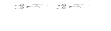
Next we look into chirality matching of the $u,d$ quarks. We first examine the case that ${\cal O}_{i}=J_{\mu}^{\dagger}J^{\mu}$ consists of left-handed currents alone. The leading quark diagram is shown in Fig. 4a. In this case, the factor $f_{\pi}p^{\mu}_{\pi}$ arises from the formation of each pion (the oval blobs in Fig. 4). Together with $m_{s}^{2}$, therefore, we obtain the large $s$ behavior of the form

$$M(s)\sim\frac{G_{F}m_{s}^{2}f_{\pi}^{2}s}{m_{K}^{2}f_{K}}$$ (9)

up to a power of $(\ln s)^{-1}$. In contrast, when ${\cal O}_{i}$ consists of left and right-handed currents as the dominant penguin operator ${\cal O}_{6}$ does, the pion is formed from a chirality-matched pair of $\overline{q_{L}}q_{R}$ or $\overline{q_{R}}q_{L}$ with the matrix element $m_{\pi}^{2}f_{\pi}/(m_{u}+m_{d})$. This type of decay dominates at low energies, e.g., on the kaon mass shell[21]. When we go to high energies, however, the absence of $p^{\mu}$ in the pion formation makes this penguin amplitude softer in $s$ dependence:

$$M(s)\sim\frac{G_{F}m_{s}^{2}f_{\pi}^{2}m_{\pi}^{4}}{m_{K}^{2}f_{K}(m_{u}+m_{d})^{2}},\;\;({\rm for}\;{\cal O}_{6}).$$ (10)

When we combine Eq. (9) or (10) with Eq. (7), we obtain $N-\delta(\infty)/\pi=1$ or 0. If the low-energy zero at $s=m_{\pi}^{2}$ is the only zero of $M(s)$, then the asymptotic phase should approach $0$ or $\pi$, depending on the asymptotic behavior of $M(s)$:

$$\delta_{0}(\infty)=\left\{\begin{array}[]{cl}0&(N=1;\;M(s)\sim s),\\ \pi&(N=1;\;M(s)\rightarrow{\rm const}).\end{array}\right.$$ (13)

The first line applies to the “tree” operator ${\cal O}_{1,2}$, while the second line is for the dominant penguin operator ${\cal O}_{6}$. We emphasize that these asymptotic behaviors are specific to the case of the PCAC in QCD. They are not necessarily applicable to effective theories for which we do not know $M(\infty)$.

For the $\Delta I=\frac{3}{2}$ decay, the pure weak decay has the zero at $s=m^{2}_{\pi}$. (Appendix B) If this is the only zero ($N=1$), we have $\delta_{2}(\infty)=0$ since $M(s)\sim s$. On the other hand the EM penguin matrix element need not vanish at $s=m_{\pi}^{2}$. The perturbative QCD argument presented above remains valid even after one internal photon line is inserted. Therefore $M(s)\sim constant$ for the dominant penguin operator ${\cal O}_{8}$. The cases of the smallest number of zeros for the $\Delta I=\frac{3}{2}$ amplitudes are, therefore,

$$\delta_{2}(\infty)=\left\{\begin{array}[]{cl}0&\;(N=1;\;M(s)\sim s)\\ 0&\;(N=0;\;M(s)\sim\;{\rm constant}),\\ -\pi&\;(N=0;M(s)\sim s).\end{array}\right.$$ (14)

The first line applies to the pure weak decay ${\cal O}_{1,2}$, while the second line is for the EM penguin ${\cal O}_{8}$.

If there are more zeros in the amplitude, $\delta_{I}(\infty)$ shifts upward from those given in Eqs. (13) and (14). The larger the value of $|\delta_{I}(\infty)|$ is, the more important the contributions from the inelastic FSI and the ISI are, as we shall see below.

V Quantitative discussion

We first define the problem to which we address in this paper: Suppose that we compute with the effective weak interaction $c_{i}(\mu){\cal O}_{i}$ the decay amplitude $M(s)$ at some small value $s_{0}$ below the $\pi\pi$ threshold. The value of such $M(s_{0})$ is real though it incorporates all the FSI and the ISI that enter through the dispersion integral of $\delta(s)$. Then we ask how much $|M(m_{K}^{2})|$ is different from $M(s_{0})$. We should keep in mind that the value of $M(m_{\pi}^{2})$ depends on choice of the kaon field in principle. Strictly speaking, therefore, this problem makes sense only after we have defined the kaon field.

We focus on the least ambiguous case that $M(s)$ has the minimum number of zeros, namely, only one zero at $s=m_{\pi}^{2}$ for all amplitudes except for the EM penguin and no zero for the EM penguin. The zero at or near $s=m_{\pi}^{2}$ is robust. In contrast, it is rather an ad hoc assumption that there is no other zero. We use the values of $\delta_{I}(\infty)$ predicted by the PCAC for the kaon, namely, $\delta_{0}(\infty)=\pi$ for the dominant gluon penguin operator of left and right-handed currents and $\delta_{2}(\infty)=0$ for the $\Delta I=\frac{3}{2}$ operators. (cf Eqs. (13) and (14).)

When $H_{W}$ is one of the effective operators $c_{i}(\mu){\cal O}_{i}$, it is reasonable to match the OM representation to the short-distance QCD by cutting off the dispersion integral at $s\simeq\mu^{2}$. Since $\mu^{2}$ is the spacelike scale of renormalization group, it would be more appropriate to make analytic continuation of $c_{i}(\mu)$ to the timelike region. This would generate an imaginary part of $O((\ln\mu)^{-1})$ relative to the real part as the high-energy tail of FSI. We can ignore it as a small correction if $\mu$ is in the perturbative regime of QCD. It has been a subject of discussion how far one can lower $\mu$ without losing desired accuracy and how one should match $c_{i}(\mu)$ to low-energy matrix element computation. If we could choose as low as $\mu=$ 1 GeV, the issues of this paper would mostly disappear since all we would need is the elastic scattering phase shifts. However, such a low cutoff is hard to justify particularly in the $I=0$ channel where the scalar resonances $f_{0}$ exist at 1500 MeV and 1700 MeV. While $\mu\simeq$ 2 GeV is probably safe, it may be possible to lower $\mu$ close to 1.5 GeV ($\simeq m_{c}$). Near $s=\mu^{2}$, $\delta(s)$ ought to approach its asymptotic value $\delta(\infty)$. Otherwise the $s$ dependence of $M(s)$ computed with the cutoff dispersion integral would not give a smooth asymptotic behavior at $s=\mu^{2}$.

Below the inelastic threshold, the phase of $M(s)$ is equal to the $s$-wave phase shift of elastic $\pi\pi$ scattering by Watson’s theorem[4]. The elastic phase shift of $I=0$ is positive and grows to large values with energy[22], while that of $I=2$ stays negative and small in magnitude. Though theoretically the inelastic scattering starts at $\sqrt{s}=4m_{\pi}$, in reality the inelasticity in the $I=0$ channel appears rather suddenly at $\sqrt{s}=2m_{K}$ where the $K\overline{K}$ channel opens. The $I=0$ scattering phase shift rapidly rises to $\pi$ across $\sqrt{s}=2m_{K}$ passing through the $f_{0}(980)$ resonance just below the $K\overline{K}$ threshold. As we have emphasized, however, the $\pi\pi$ scattering phase shift above $\sqrt{s}=2m_{K}$ has little to do with the phase of the $K\rightarrow\pi\pi$ decay amplitude: Once an inelastic channel opens, the phase theorem no longer relates the two phases since the latter depends on the relative sign and magnitude of the $K\rightarrow K\overline{K}$ transition matrix element to the $K\rightarrow\pi\pi$ decay amplitude too, as we shall see below. Therefore the surge of the $\pi\pi$ scattering phase shift across $\sqrt{s}=2m_{K}$ does not necessarily means that the phase $\delta_{0}(s)$ of $M(s)$ rises abruptly in the same way. In fact, when an elastic channel strongly couples to an inelastic channel, a partial wave amplitude moves quickly toward the center of the Argand diagram and its scattering phase shift often undergoes a rapid variation across the inelastic threshold. It is quite possible that the phase $\delta_{0}(s)$ of $M(s)$ varies more slowly across $\sqrt{s}=2m_{K}$ than the $\pi\pi$ scattering phase shift does.

With the asymptotic values of $\delta_{0}(\infty)=\pi$ and $\delta_{2}(\infty)=0$ (cf Eqs. (13) and (14), we have drawn schematically the behaviors of the phase $\delta_{I}(s)$ of $M(s)$ up to $s=\mu$($\simeq$ 2 GeV) in Fig. 5a by smoothly interpolating between $\sqrt{s}=2m_{K}$ and $\mu$.

A Inelastic FSI and ISI

The phase $\delta_{I}(s)$ above the inelastic threshold comes from the ISI and the inelastic FSI. For curiosity, we have actually computed the diagrams that generate the lowest singularities in the OM representation (Fig. 2a and 2c). The FSI contribution of the diagram in Fig. 2a to the absorptive part ${\rm Im}M(s)$ of $I_{\pi\pi}=0$ is:

$${\rm Im}M^{K\overline{K}}(s)=\biggl{(}\frac{g^{2}_{K^{*}K\pi}}{4\pi}\biggr{)}\sqrt{\frac{s-4m_{K}^{2}}{s}}I(s)\kappa(s){\rm Re}M(s),$$ (15)

where $\kappa(s)$ is the ratio of the $K\rightarrow K\overline{K}$ amplitude of ${\Delta I=1/2}$ to the $K\rightarrow\pi\pi$ amplitude of ${\Delta I=1/2}$ at $\sqrt{s}$, $g^{2}_{K^{*}K\pi}/4\pi\simeq 1.3$ is the $K^{*}K\pi$ coupling, and $I(s)$ is a known logarithmic function of $\sqrt{s}$. We have chosen $\frac{1}{2}\sum(|out\rangle\langle out|)+|in\rangle\langle in|)$ for the intermediate states in order to ensure the absorptive part to be real. For a numerical estimate of the magnitude, let us choose some value for $\sqrt{s}$, say, $\sqrt{s}=2.5m_{K}(\simeq 1.25$ GeV), for which $I(s)\simeq 0.50$. We set $\kappa(s)=(s-m_{K}^{2})/(s-m_{\pi}^{2})$, which is the prediction of the octet dominance for $H_{W}$ and SU(3) symmetry for strong interactions. Then we find

$${\rm Im}M^{K\overline{K}}\simeq 0.39\times{\rm Re}M\;\;({\rm at}\;\sqrt{s}=2.5m_{K}).$$ (16)

At higher $\sqrt{s}$, the states such as $\eta\eta$, $a_{1}\pi$, and $\rho\rho$ become important intermediate states. While reliable estimate is less easy for those decay modes, the inelastic FSI of $K\rightarrow K\overline{K}\rightarrow\pi\pi$ appears sizable.

Let us turn to the ISI of the diagram of Fig. 2c which generates the lowest ISI singularity. There are two independent $\Delta I=\frac{1}{2}$ transitions for $K^{*}\rightarrow\rho\pi$:

$$a(\mbox{\boldmath$\pi$}\cdot\mbox{\boldmath$\rho$})(\overline{K}S)+b(\mbox{\boldmath$\pi$}\times\mbox{\boldmath$\rho$})\cdot(\overline{K}\mbox{\boldmath$\tau$}S)+h.c.,$$ (17)

where $S=(0,1)$ represents the $\Delta I=\frac{1}{2}$ spurion. The first term of Eq. (17) cancels out in the diagram of Fig. 2c by the isospin structure. The second term gives

$${\rm Im}M^{K^{*}\pi}(s)=\biggl{(}\frac{g_{K*K\pi}g_{\rho\pi\pi}}{4\pi}\biggr{)}\bigg{(}\frac{2|{\bf q}|}{\sqrt{s}}\biggr{)}\lambda(s)J(s){\rm Re}M(s),$$ (18)

where $\lambda(s)$ is the ratio $b/{\rm Re}M(s)$, ${\bf q}$ is the c.m. momentum of $K^{*}\pi$, and $J(s)$ is another known function of $\sqrt{s}$. In contrast to the case of the inelastic FSI of the $K\overline{K}$ intermediate state above, we know little about the value of $\lambda(s)$. For $\lambda(s)\approx 1$ we obtain at $\sqrt{s}=2.5m_{K}$ ($J(s)\simeq 0.36$)

$${\rm Im}M_{0}^{K^{*}\pi}\approx 0.27\times{\rm Re}M_{0}\;\;({\rm at}\;\sqrt{s}=2.5m_{K}),$$ (19)

The ISI is not negligible either though Eq. (19) gives only an order-of-magnitude estimate at best. The intermediate states $\rho K$, $\omega K$, and so forth start contributing to the ISI at a little above $\sqrt{s}=2.5m_{K}$.

This exploratory numerical exercise indicates that both the ISI and the inelastic FSI are large enough to deserve study. Since computation by individual diagrams involves too many uncertainties, we instead attempt to extract general trends and some quantitative results with minimal assumptions.

B $I=0$ channel

We estimate the variation $M(m_{K}^{2})-M(s_{0})$ for the dominant gluon penguin decay with $\delta_{0}(s)$ of Fig. 5a. We choose $s_{0}$ at the SU(3)-symmetry point $m_{\pi}^{2}$ and quote the variation due to the exponential in the $\pi\pi$ isospin channel $I$ after separating out the factor $(s-m_{\pi}^{2})$:

$$M_{I}(s) \equiv (s-m_{\pi}^{2})\tilde{M}_{I}(s)$$ (20)

$${\cal R}_{I} = |\tilde{M}_{I}(m_{K}^{2})|/\tilde{M}_{I}(m_{\pi}^{2}).$$ (21)

The result is

$${\cal R}_{0}\simeq\left\{\begin{array}[]{cl}1.50&(\mu=1.5\;{\rm GeV}),\\ 1.57&(\mu=2\;{\rm GeV})\end{array}\right.$$ (22)

The subtraction in the dispersion integral suppresses the contribution from the high-energy tail at 1.5 GeV $<\sqrt{s}<$ 2 GeV. The authors of Ref.[3] quoted ${\cal R}_{0}=1.41\pm 0.06$ without including the contribution above the inelastic threshold. We can estimate the effect of the ISI and the inelastic FSI by evaluating the phase integral above $\sqrt{s}=2m_{K}$ separately from the elastic region $\sqrt{s}\leq 2m_{K}$. The contribution from the ISI and the inelastic FSI is:

$${\cal R}_{0}^{ISI+IFSI}=\left\{\begin{array}[]{cl}1.13&(\mu=1.5\;{\rm GeV}),\\ 1.18&(\mu=2\;{\rm GeV}).\end{array}\right.$$ (23)

The ISI and the inelastic FSI combined contribute to the variation of $M_{0}(s)$ by a third to one half of the elastic FSI. The sizable contribution above the inelastic threshold means that we cannot truncate the integral at $\mu=$ 1 GeV and connect to short-distance calculations. This is an unfortunate situation since we cannot obtain the values of $\delta_{0}(s)$ at $2m_{K}<\sqrt{s}<\mu$ directly from experiment. For comparison we have made an estimate in the case that $\delta_{0}(s)$ follows the behavior of the $\pi\pi$ phase shift across the $K\overline{K}$ threshold. (see the broken curve in Fig. 5a.) The value of ${\cal R}_{0}^{ISI+IFSI}$ in this case is:

$${\cal R}_{0}^{ISI+IFSI}=\left\{\begin{array}[]{cl}1.17&(\mu=1.5\;{\rm GeV}),\\ 1.23&(\mu=2\;{\rm GeV}).\end{array}\right.$$ (24)

Though the ISI and the inelastic FSI are important, their magnitudes are not highly sensitive to the $s$ dependence of $\delta_{0}(s)$. As we shall see below, it is the value of $\delta_{0}(\infty)$, namely, the number of zeros of the amplitude that they are more sensitive to.

C I=2 channel

We consider the case of $\delta_{2}(\infty)=0$ for the pure weak decay ($N=1$) and the EM penguin decay ($N=0$). Because of the large enhancement of the $\Delta I=\frac{1}{2}$ decay over the $\Delta I=\frac{3}{2}$ decay, the $I=2$ channel of $K_{S}$ may receive a sizable $\Delta I=\frac{3}{2}$ contribution from an enhanced $\Delta I=\frac{1}{2}$ decay followed or preceded by long-distance electromagnetic isospin breaking, e.g., $\pi$-$\eta$ mixing. Such a contribution may compete with the pure weak decay and the EM penguin decay in the $\Delta I=\frac{3}{2}$ decay. For the $\Delta I=\frac{3}{2}$ decay generated by long-distance electromagnetic corrections, however, $\delta_{2}(s)$ of $M_{2}(s)$ is no longer equal to the $\pi\pi$ scattering phase shift of $I=2$ nor $I=0$ even below $\sqrt{s}=2m_{K}$.

When we ignore the long-distance electromagnetic correction and use $\delta_{2}(s)$ of Fig. 5a, the numbers corresponding to Eqs. (22) and (23) are:

$${\cal R}_{2}=0.91\;(\mu=1.5\;{\rm GeV}),$$ (25)

and

$${\cal R}_{2}^{ISI+IFSI}=0.99\;(\mu=1.5\;{\rm GeV}).$$ (26)

Our numbers are in perfect agreement with ${\cal R}_{2}\simeq 0.92\pm 0.02$ obtained in [3]. However there is no factor of $(s-m_{\pi}^{2})$ for the $\Delta I=\frac{3}{2}$ EM penguin decay. The contribution from above 1 GeV is much smaller in $I=2$ than in $I=0$ because of $\delta_{2}(\infty)=0$. For the same reason, dependence on the value of $\mu$ is very mild. For the EM penguin operators ${\cal O}_{9,10}$, $M(s)\sim s$ so that the asymptotic phase would be $\delta_{2}(\infty)=-\pi$ (cf Eq. (14)). In this case we obtain a stronger suppression. It should be emphasized again that Eq. (25) does not apply to long-distance electromagnetic corrections to the gluon penguin operator decay, since we cannot equate $\delta_{2}(s)$ of $M_{2}(s)$ to a $\pi\pi$ scattering phase shift even in the elastic region. The OM representation is practically useless in this case.

D More zeros ($N\geq 2$)

When $M_{0}(s)$ has more than one zero, the asymptotic value $\delta_{0}(\infty)$ is larger. Consider the case that $M_{0}(s)$ has one more zero ($N=2$). In this case $\delta_{0}(\infty)=2\pi$. The second zero must be located on the real axis in order to be consistent with real analyticity $M(s^{*})=M(s)^{*}$. The zero at $s=m_{\pi}^{2}$ is obtained in the Taylor expansion to $O(p^{2})$ with SU(3) symmetry. When we include $O(p^{4})$, the location of this zero stays as long as SU(3) symmetry is maintained, but another zero emerges. If the second zero is outside the soft-meson region, we cannot trust its presence. If it is inside or close to the soft-meson region, it means that the next-order terms are important at low energies. If the lowest-order chiral Lagrangians give a good description of $K$ decays, the second zero should be far from the soft-meson region and therefore the second zero factor $(s-s_{2})$ would not generate very rapid variations at low energies. Our hope is that the dominant penguin operator has no second zero and reaches its asymptopia quickly. If the second zero exists in the region of $|s|=O(16\pi^{2}\Lambda_{QCD}^{2})$, the variation due to the second zero factor $(s-s_{2})$ could be substantial when we extrapolate from $s=m_{\pi}^{2}$ to $m_{K}^{2}$. Lack of our knowledge of its precise location introduces a large uncertainty in the extrapolation.

If we assume that $\delta_{0}(s)$ rises linearly in $\sqrt{s}$ to $2\pi$ from 1 GeV to 2 GeV (Fig. 5b), the ratio of the exponential factors at $s=m_{K}^{2}$ and $m_{\pi}^{2}$ after removing $(s-m_{\pi}^{2})(s-s_{2})$ is:

$${\cal R}_{0}=1.64\;(\mu=2\;{\rm GeV}).$$ (27)

In comparison, if $\delta_{0}(s)$ follows the inelastic behavior of $\pi\pi$ scattering phase shift (the broken curve in Fig. 5b), the corresponding value could be:

$${\cal R}_{0}=1.83\;(\mu=2\;{\rm GeV}).$$ (28)

In the case of two zeros, therefore, the ISI and inelastic FSI contribution can be as large as or even larger than the elastic FSI contribution.

If $M(s)$ has three zeros, the second and third zeros can appear off the real axis in a complex conjugate pair. After we include the variation due to the factor $\prod_{i}(s-s_{i})$, the uncertainties get quickly out of control as $N$ increases. The uncertainty due to the number of zeros and their locations appears to be by far the largest.

VI Conclusion

We have studied with the Omnès-Muskhelishvili representation the off-shell kaon mass dependence of the $K\rightarrow\pi\pi$ decay amplitudes for the purpose of exposing the uncertainties that have so far not been seriously studied. Determining the phases above the inelastic threshold encounters two difficulties. One is complexity of inelastic rescattering and the other is physical nonuniqueness of off-shell amplitudes in general. In this paper we have studied the off-shell behavior with QCD as the underlying fundamental theory and with the PCAC for the extrapolated kaon field. As it is suspected, the largest uncertainty is how many zeros exist in the amplitudes and where they are located. We regret that we cannot be optimistic in our conclusion as to accuracy or certainty of the off-shell extrapolation. If we work in the spurion scattering formalism where all hadrons are on shell, we do not encounter the physical nonuniquness due to off-shellness. However, evaluation of the dispersion relation is equally formidable since it requires knowledge of the hadron-spurion scattering with the spurion carrying nonvanishing energy-momentum. In either approach, we are unable to work only with physical quantities directly measurable in experiment. If we were able to lower the cutoff to $\mu=$ 1 GeV, we could do without the inelastic region. However, this does not seem possible since $\delta_{0}(s)$ is not yet asymptotic at 1 GeV.

If we have very accurate knowledge of $M(s)$ in the low-energy region, we can suppress the large $s$ portion of the integral by writing a phase dispersion integral with more than one low-energy subtraction[3]. In this case the low-energy values of $M(s)$ that we feed in the dispersion relation would incorporate implicitly the contribution from inelastic region. The problem would then reduce to determining the physically unique value of $M(m_{K}^{2})$ with the elastic phase shift and with the off-shell values of $|M(s)|$ which are well defined only after field theory is specified for mesons. Though the physical nonuniqueness of the off-shell $|M(s)|$ should, in principle, cancel out in $M(m_{K}^{2})$, it is not clear whether we can obtain, in practice, accurate enough low-energy values of $M(s)$ from higher-order chiral Lagrangian terms.

Our final comment is on the implications of our study in $B$ decay. The FSI is highly inelastic on the $B$ mass shell and the ISI starts at $s=(m_{B^{*}}+m_{\pi})^{2}$, right above the $B$ mass. Unless short-distance strong interactions completely dominate in the FSI and the ISI, computation of magnitudes of decay amplitudes would be subject to very large uncertainties, far more than in $K$ decay. Several theoretical arguments have been presented in favor of short-distance dominance after factorization. Nevertheless, if we should find from experiment an FSI phase much larger than the short-distance prediction in some decay mode, our work here would be telling us that it is almost hopeless to compute such a decay amplitude with decent accuracy.

A Phase in the presence of inelasticity

Many of us are aware that the phase of decay amplitude is not determined by strong interaction alone at energies where inelastic rescattering occurs. Its value is an outcome of complicated interplay between strong and weak interactions. Sicne there is some confusion on this important point in literature, we clarify it in the simplest possible term here.

Consider the decay amplitude for $A\rightarrow a+b$ at energies where scattering of $a+b$ is inelastic in general. The partial-wave S-matrix of strong interaction scattering is diagonalized by eigenchannels:

$$\langle n^{out}|n^{\prime in}\rangle=\delta_{nn^{\prime}}e^{2i\delta_{n}}.$$ (A1)

Making time reversal on $\langle n^{out}|H_{w}|A\rangle$, we obtain for T-invariant $H_{W}$

$$\langle n^{out}|H_{W}|A\rangle = \langle A|H_{W}|n^{in}\rangle,$$ (A2)

$$= \langle A|H_{W}|n^{out}\rangle\langle n^{out}|n^{in}\rangle,$$ (A3)

$$= e^{2i\delta_{n}}\langle A|H_{W}|n^{out}\rangle.$$ (A4)

With $\langle A|H_{W}|n^{out}\rangle=\langle n^{out}|H_{W}|A\rangle^{*}$, this relation leads us to

$$M_{n}(s)=\overline{M}_{n}(s)e^{i\delta_{n}(s)},$$ (A5)

where $\overline{M}_{n}(s)$ is real. This is the phase theorem referred to as Watson’s theorem or, to be more precise[24], the Watson-Fermi-Aizu theorem. At energies where only one eigenchannel is open in the final state, the phase of a matrix element for any operator having the same quantum numbers as $H_{W}$ is universal and equal to the scattering phase shift.

However, the situation is different at energies where inelastic channels are open and a final state is not an eigenchannel of scattering. Because of T-invariance of strong interaction, the transformation between $|ab\rangle$ and eigenchannels $|n\rangle$ can be chosen as orthogonal:

$$|ab^{out}\rangle=\sum_{n}O_{ab,n}|n^{out}\rangle,\;\;(O^{*}_{ab,n}=O_{ab,n}).$$ (A6)

Therefore the decay amplitude $M_{ab}$ into the observable final state $|ab\rangle$ takes the form

$$M_{ab}(s)=\sum_{n}O_{ab,n}(s)\overline{M}_{n}(s)e^{i\delta_{n}(s)}.$$ (A7)

The net phase of $M_{ab}(s)$ results from a superposition of the eigenphase shifts weighted with the orthogonal transformation matrix elements $O_{ab,n}(s)$ and the weak decay amplitudes $\overline{M}_{n}(s)$ into the eigenchannels.

In contrast, the phase shift $\delta_{ab}$ of scattering $a+b\rightarrow a+b$ in the presence of inelasticity is defined with the inelasticity $\eta_{ab}$ by $\langle ab^{out}|ab^{in}\rangle\equiv\eta_{ab}e^{2i\delta_{ab}}$[25]. Therefore,

$$\eta_{ab}e^{2i\delta_{ab}}=\sum_{n}O_{ab,n}^{2}e^{2i\delta_{n}}.$$ (A8)

The phase $\delta_{ab}$ is a quantity determined by strong interactions alone. Above the inelastic threshold the phase of the decay amplitude $M(s)_{ab}$ has nothing to do with the strong interaction phase shift.

B Low-energy zeros

It is straightforward to extend the theorem by Cabibbo and Gell-Mann [13] to the $\Delta I=\frac{3}{2}$ decay of $K\rightarrow\pi\pi$ and show that the $\Delta I=\frac{3}{2}$ amplitude also vanishes in the SU(3) limit of strong interaction. We reconstruct the extension of the proof and show the robustness of the low-energy zero.

When $H_{W}$ is the current-current interaction in a symmetric product of two octet $V-A$ currents, it forms $\{8_{S}\}$ and $\{27\}$. Using the SU(3) tensor notation (1,2,3) for ($u,d,s$), we can express the transformation property of $H_{W}$ as

$$H_{W}\sim H^{12}_{31}+H^{31}_{12},$$ (B1)

where the upper and lower pairs of indices are both symmetric under interchange. To remove $\{8_{S}\}$ from the right-hand side, we should subtract the trace portion. But it is not necessary here since the theorem was already proven for the octet spurion. The relative sign of $H^{12}_{31}$ and $H^{31}_{12}$ is positive. In the case of $\{8_{S}\}$ this relative sign aligns $H_{W}$ along $\lambda_{6}$ instead of $\lambda_{7}$. It is crucial to the proof of the theorem for the ${\{27\}}$ spurion as well.

We parametrize the $0^{-}\rightarrow 0^{-}+0^{-}$ decay matrix elements of $\{27\}$ without derivatives in terms of the $3\times 3$ octet meson matrix $M$, instead of $U=\exp(i\lambda_{a}\phi_{a}/f_{\pi})$ of SU(3)${}_{L}\times SU(3)_{R}$:

$${\cal M}=(M^{1}_{i}M^{i}_{3}M^{2}_{1}+M^{i}_{1}M^{3}_{i}M^{1}_{2})+(1\leftrightarrow 2)+(3\leftrightarrow 1)+(1\leftrightarrow 2,\;3\leftrightarrow 1).$$ (B2)

The relative sign within each bracket is positive, as pointed out above. Otherwise ${\cal M}$ would point along a wrong component of $\{27\}$.

The parity-violating part of $H_{W}$ is odd under charge conjugation C when $H_{W}$ is (approximately) CP invariant. That is, $H^{12}_{31}\rightarrow-H^{31}_{12}$ under C for $H_{W}^{{\rm pv}}$. It means that the $\{27\}$ (and also $\{8_{S}\}$) made of symmetric products of the $V$ and $A$ currents must be a ${\cal C}$-odd multiplet of SU(3). Since $M\rightarrow M^{T}$ ($T$ = transposed) under C, all terms in Eq. (B2) transform into each other such that ${\cal M}\rightarrow+{\cal M}$. Namely, ${\cal M}$ can make only a ${\cal C}$-even $\{27\}$. Therefore, we cannot construct an SU(3) covariant matrix element having the correct charge conjugation property.

It is obvious in the chiral Lagrangian approach that one cannot write nonderivative Lagrangian terms for $\{8\}_{L}$ nor $\{27\}_{L}$ of $H_{W}$. However, chiral symmetry is not really needed to prove the theorem; the original proof by Cabibbo and Gell-Mann never used it.

The theorem fails once SU(3) breaking is included. The decay spurion arising from $H_{W}$ with the electromagnetic interaction or the quark mass difference is no longer a symmetrized product of two octets. The EM penguin contains $\{10\}$, and $\{\overline{10}\}$ too.

The thereom is valid even after derivatives are included for the mesons: $M\partial_{\mu}M\partial^{\mu}M$ generates $(p_{2}\cdot p_{3})$, which is equal to $(p_{1}^{2}-p_{2}^{2}-p_{3}^{2})/2$ and reduces to a common value $-p^{2}/2$ at the SU(3)-symmetry point, $p_{1}^{2}=p_{2}^{2}=p_{3}^{2}=p^{2}$. Therefore all contracted pairs of derivatives are factored out as SU(3) invariants so that the SU(3) symmetry property of $M\partial_{\mu}M\partial^{\mu}M$ is identical with that of $MMM$.

Given this theorem, the off-shell $K\rightarrow\pi\pi$ amplitude to $O(p^{2})$ is unique up to a proportionality constant. To prove it, write the off-shell amplitude as a function of $p_{a}^{2}$, $p_{b}^{2}$, and $p_{K}^{2}$ by incorporating the Bose statistics for the final $\pi_{a}\pi_{b}$ in $s$-wave:

$${\cal M}=A(p_{a}^{2}+p_{b}^{2})+Bp_{K}^{2}+O(p^{4}).$$ (B3)

In order for ${\cal M}$ to vanish at the SU(3) symmetry point, $B$ must be equal to $-2A$. Consequently, ${\cal M}=-A(2p_{K}^{2}-p_{a}^{2}-p_{b}^{2})$. This argument applies to both $\{8\}$ and $\{27\}$.

All we need for the proof is $M\rightarrow+M^{T}$ and the fact that $\Delta I=\frac{3}{2}$ of $H_{W}^{{\rm pv}}$ is a ${\cal C}$-odd $\{27\}$. Therefore, even if the extrapolation fields of $0^{-}$ mesons did not respect chiral symmetry off mass shell, the theorem would be valid. It is a misnomer to refer to the zero at $s=m_{\pi}^{2}$ as the “chiral zero”.

FIG. 1.: Analyticity of the spurion scattering amplitude off $K$ into $\pi\pi$.

FIG. 2.: (a) An inelastic FSI diagram. (b) The ISI diagram of the nearest left-hand singularity. (c) Another ISI diagram, which produces the lowest two-body ISI cut in the OM representation.

FIG. 3.: The $s$-plane singularity of the OM representation.

FIG. 4.: The quark diagrams for $K\rightarrow\pi\pi$ through (a) the decay operator which contains only left-handed currents and (b) the decay operator which contains both left and right currents. $L(\overline{L})$ and $R(\overline{R})$ denote the left-chiral and the right-chiral quark, respectively, of $u,d$ flavors (their anti-particles).

FIG. 5.: (a) A schematic drawing of the behaviors of $\delta_{I}(s)$ for $I=0$ and $I=2$ with the asymptotic values $\delta_{0}(\infty)=\pi$ and $\delta_{2}(\infty)=0$, respectively. The broken curve is for the case where $\delta_{0}(s)$ behaves like the $\pi\pi$ phase shift across $\sqrt{s}=2m_{K}$. (b) $\delta_{0}(s)$ in the case of $\delta_{0}(\infty)=2\pi$ ($N$=2).

REFERENCES

- [1] T. N. Truong, Phys. Lett. 207B, 495 (1988); 313B, 221 (1993).
- [2] N. Isgur, K. Maltman, J. Weinstein, and T. Barnes, Phys. Rev. Lett. 64, 161 (1990).
- [3] E. Palante and A. Pich, Phys. Rev. Lett. 84, 2526 (2000); hep-ph/0007208 and references therein.
- [4] K. M. Watson, Phys. Rev. 95, 228 (1954); K. Aizu, Proceedings of Int. Conf. Theoret. Phys. 1953, (Kyoto-Tokyo Science Council, 1954), p.200; E. Fermi, Suppl. Nuovo Cim. 2, 58 (1955); J. Gillespie, Final-State Interactions (Holden-Day, San Francisco, 1964).
- [5] N. I. Muskhelishvili, Singular Integral Equations (Noordhoof, Gronigen, 1953) p.204; R. Omnès, Nuovo Cim, 8, 316 (1958).
- [6] N. Levinson, Danske Videnskab. Selskab. Mat.-fys. Medd., 25, No.9 (1949).
- [7] S. R. Chisholm,26, 469 (1961): S. Kamefuchi, O’Raifeartaigh, and A. Salam, Nucl. Phys. 28, 529 (1961).
- [8] A. J. Buras, M. Ciuchini, E. Franco, G. Ishidori, G. Martinelli, and L. Silvestrini, hep-ph/0002116.
- [9] T. N. Truong, hep-ph/0101345 discusses some basic aspects.
- [10] H. Lehmann, K. Symanzik, and W. Zimmermann, Nuovo Cim. 1, 42 (1955).
- [11] R. J. Eden, P. V. Landshoff, D. Olive, and J. C. Polkinghorne, Analytic S-matrix (Cambridge Univ. Press, Cambridge, 1965) and references therein.
- [12] R. Jost, Helv. Phys. Acta 20, 256 and 22, 256 (1947). R. Jost and A. Pais, Phys. Rev. 82, 840 (1951); R. Jost and W. Kohn, Phys. Rev. 87, 977 (1952).
- [13] N. Cabibbo, Phys. Rev. Lett. 12, 62 (1964); M. Gell-Mann, Phys. Rev. Lett. 12, 155 (1964). See Appendix B for extension to .
- [14] The off-shell behavior was computed with the -model by J. A. Cronin, Phys. Rev. 161 1483 (1967). See for earlier works by current algebras: M. Suzuki, Phys. Rev. 144, 1154 (1966); S. K. Bose and S. N. Biswas, Phys. Rev. Lett. 16, 330 (1966); Y. Hara and Y. Nambu, Phys. Rev. Lett. 16, 875 (1966); J. C. Taylor, Nuovo Cim. 44, 518 (1966); B. M. Nefkins, Phys. Lett. 22, 94 (1966).
- [15] J. Schwinger, Phys. Lett. 24B, 473 (1967).
- [16] C. G. Callan, S. Coleman, J. Wess, and B. Zumino, Phys. Rev. 177, 2247 (1969).
- [17] For possibility of even more general realizations, see Bando, T. Kugo, and K. Yamawaki, Phys. Rep. 164, 218 (1988).
- [18] S. Weinberg, Phys. Rev. Lett. 18, 188 (1967).
- [19] S. Drell and F. Zachariasen, Electromagnetic Structure of Nucleons (Oxford Univ. Press, Oxford, 1961), pp.74-77.
- [20] See, for instance, G. P. Lepage and S. Brodsky, Phys. Rev. D 21, 2157 (1980).
- [21] G. Buchalla, A. J. Buras, and M. E. Lautenbacher, Nucl. Phys. B370, 69 (1992); Rev. Mod. Phys. 68, 1125 (1996); A. J. Buras, M. Jamin, and M. E. Lautenbacher, Nucl. Phys. B408, 209 (1993).
- [22] G. Grayer et al., Nucl. Phys. B75, 189 (1974); L. Rosselet et al., Phys. Rev. D 15, 5154 (1977); W. Hoogland et al., Nucl. Phys. B126, 109 (1977). See also B. S. Zou and D. V. Bugg, Phys. Rev. D 48, R3948 (1993); A. Shenk, Nucl. Phys. B363, 97 (1991).
- [23] J. F. Donoghue, E. Golowich, B. R. Holstein, and J. Trampetic, Phys. Lett. 179B, 361 (1986); A. Buras and M. Gérard, Phys. Lett. 192B, 156 (1987); H.-Y. Cheng, Phys. Lett. 201B, 155 (1988); M. Lusignoli, Nucl. Phys. B325, 33 (1989); G. Ecker, G. Müller, H. Neufeld, and A. Pich, Phys. Lett. 477B, 88 (2000); V. Cirigliano, J. F. Donoghue, and E. Golowich, hep-ph/0008290.
- [24] S. Gasiorowicz, Elementary Particle Physics, (John Wiley and Sons, New York, 1966), p.449.
- [25] H. Pilkuhn, The Interactions of Hadrons, (North Holland, Amsterdam, 1967), p.46.