An Analysis of the Next-to-Leading Order
Corrections to the $g_{T}(=g_{1}+g_{2})$ Scaling Function

Abstract

We present a general method for obtaining the quantum chromodynamical radiative corrections to the higher-twist (power-suppressed) contributions to inclusive deep-inelastic scattering in terms of light-cone correlation functions of the fundamental fields of quantum chromodynamics. Using this procedure, we calculate the previously unknown ${\cal O}(\alpha_{s})$ corrections to the twist-three part of the spin scaling function $g_{T}(x_{B},Q^{2})(=g_{1}(x_{B},Q^{2})+g_{2}(x_{B},Q^{2}))$ and the corresponding forward Compton amplitude $S_{T}(\nu,Q^{2})$. Expanding our result about the unphysical point $x_{B}=\infty$, we arrive at an operator product expansion of the nonlocal product of two electromagnetic current operators involving twist-two and -three operators valid to ${\cal O}(\alpha_{s})$ for forward matrix elements. We find that the Wandzura-Wilczek relation between $g_{1}(x_{B},Q^{2})$ and the twist-two part of $g_{T}(x_{B},Q^{2})$ is respected in both the singlet and non-singlet sectors at this order, and argue its validity to all orders. The large-$N_{c}$ limit does not appreciably simplify the twist-three Wilson coefficients.

I Introduction

Deep-inelastic scattering (DIS) of leptons on the nucleon is a time-honored example of the success of perturbative quantum chromodynamics (PQCD)[1]. The factorization formulae for the scaling functions $F_{1}(x_{B},Q^{2})$ and $g_{1}(x_{B},Q^{2})$ (defined from the Bjorken limit of the structure functions $W_{1}(\nu,Q^{2})$ and $G_{1}(\nu,Q^{2})$, respectively), augmented by the Dokshitzer- Gribov-Lipatov-Altarelli-Parisi (DGLAP) evolution equations for parton distributions [2], describe the available DIS data collected over the last 30 years exceedingly well [3]. Although the same formalism is believed to work for the so-called higher-twist structure functions [4], e.g. $W_{L}(\nu,Q^{2})$ and $G_{2}(\nu,Q^{2})$, and their associated scaling functions, $F_{L}(x_{B},Q^{2})$ and $g_{2}(x_{B},Q^{2})$, which contribute to physical observables down by powers of the hard momentum $Q$, there are few detailed studies of them in the literature beyond the tree level. [Actually, $F_{L}(x_{B},Q^{2})$ receives an $\alpha_{s}$-suppressed twist-two contribution which we will ignore in this paper.] The QCD radiative corrections to $F_{L}(x_{B},Q^{2})$ and $g_{2}(x_{B},Q^{2})$ need be investigated as accurate data have recently been taken [5, 6] and more data will be available in the future [7].

In this paper, we present a general method for obtaining radiative corrections to the higher-twist parts of structure functions in inclusive DIS. This method is based on a generalization of the tree-level formalism for higher-twist structure functions presented in Ref. [8], and has been outlined in a short paper of ours published earlier [9]. From this, we extract a straightforward set of rules which can be used to calculate the amplitude of inclusive DIS at an arbitrary order in $\alpha_{s}$ and $\Lambda_{\rm QCD}/Q$, where $\Lambda_{\rm QCD}$ is the QCD scale, in terms of light-cone correlation functions of quarks and gluons. As an illustration of our method, we present a detailed calculation of the radiative corrections to the lowest higher-twist observable, $G_{2}(\nu,Q^{2})$. The partial results of this calculation have been communicated earlier in Refs. [9, 10].

In inclusive polarized deep-inelastic scattering off a nucleon target, one can measure the spin-dependent structure functions $G_{1,2}(\nu,Q^{2})$. $G_{1}(\nu,Q^{2})$ is closely related to the spin structure of the nucleon, and has been studied extensively, both experimentally and theoretically, in the last few decades[11]. For quite a long period, the physics associated with $G_{2}(\nu,Q^{2})$, in particular the scattering mechanism and its role in understanding the internal structure of the nucleon, has generated much debate in the literature [12]. In earlier investigations, attempts were made to interpret the structure function using the naive parton model and its various extensions [13]. However, further studies showed that those results are incompatible with the factorization theorems of QCD [14]. Indeed, a QCD investigation shows that the scaling function $g_{2}(x_{B},Q^{2})$ arises from the effects of parton transverse momentum and coherent parton scattering. The new information about the nucleon structure contained in $G_{2}(\nu,Q^{2})$ is found in its twist-three part [15], which reflects the quark-gluon correlations in the nucleon. In fact, this structure function represents the simplest manifestation of these correlations found in experiment. In addition, much of the information contained in $G_{2}(\nu,Q^{2})$ has phenomenological interest. For example, the third moment of its scaling function, $g_{2}(x_{B},Q^{2})$, is related to the response of the chromo-electric and -magnetic fields inside the nucleon to its spin polarization [16]. This information can help us to understand the role of the gluon fields in the nucleon, to test lattice QCD calculations, and to construct more accurate models of nucleon structure.

It is useful at this point to remind the reader of a fey key developments in studying the $G_{2}$ structure function. Before QCD was invented, Burkhardt and Cottingham derived the super-convergence sum rule $\int d\nu\,G_{2}(\nu,Q^{2})=0$ based on a dispersion relation and an assumption about asymptotic properties of the related Compton amplitude [17]. In the context of QCD, a number of issues about $G_{2}(\nu,Q^{2})$ have been clarified in recent years. At tree level, $g_{2}(x_{B},Q^{2})$ is related to a seemingly simple quark distribution, $q_{T}(x,Q^{2})$, within the nucleon [18]. However, as first pointed out by Shuryak and Vainshtein [19], its leading-log evolution reveals this simple form to be deceptive. In reality, one requires the introduction of a more general distribution to obtain a closed evolution equation [20]. As found by Ali, Braun, and Hiller [21], a somewhat surprising simplification occurs in the limit of large number of colors. In this limit, the leading order evolution of $q_{T}(x,Q^{2})$ becomes autonomous in the nonsinglet sector. However, it was later argued that this simplification does not occur at higher orders or in the singlet sector [22]. An analysis of the local operators associated with the tree-level expressions for the moments of $g_{2}(x_{B},Q^{2})$ reveals a relation between its twist-two part and the scaling function $g_{1}(x_{B},Q^{2})$ [23]. This relation makes it possible to extract the twist-three part of $g_{2}(x_{B},Q^{2})$ from the data. Experimental measurements of $G_{2}$ have been made by a number of collaborations [24]. In addition, model calculations and lattice QCD yield interesting insights of the twist-three part of the structure function [25].

This paper is organized as follows. In Section 2, a general discussion of the kinematics and structure functions associated with spin-dependent inclusive DIS is made. This section serves to familiarize the reader with some of our conventions and notations. Section 3 is broken into five subsections dedicated to a systematic presentation of the method we use to obtain radiative corrections to the power-suppressed contributions to our amplitude. First, we summarize the well-known light-cone power counting techniques to the process at hand, which allows us to organize contributions to the amplitude with respect to their power suppression. Then, we discuss the role of longitudinal gluons in this process and the simplifications associated with the light-cone gauge. This is followed by a simple example in which the known tree-level result for $G_{2}(\nu,Q^{2})$ is derived. It is here that the nonsinglet distributions in inclusive DIS with transverse polarization are introduced. Subsection D discusses the subtleties of renormalization and factorization relevant to radiative corrections. The last subsection presents a set of rules derived from this method which can be used to obtain the contribution to inclusive DIS at an arbitrary order in $1/Q$ and $\alpha_{s}(Q^{2})$. In Section 4, we apply this method to the one-loop corrections of the results in Section 3C in the non-singlet and singlet sectors. These results were first presented in Refs. [9, 10]; in the present communication, we go into somewhat more detail in explaining their derivation. An earlier analysis of the one-loop corrections in the singlet sector can be found in Ref.[26]. Although the preliminary amplitudes are the same, the final answer and its interpretation are quite different. A recent study of these corrections [27] presents the same interpretation found here. There, one can also find discussions of the numerical significance of the results. Section 5 presents the results of the last section in the form of an operator product expansion. In this form, it is easy to exploit the full space-time symmetries of our theory and isolate the new information provided by transverse scattering. This is one of the main results of this paper, as the twist-three Wilson coefficients have never been obtained at one-loop order before. In Section 6, we explain how to perform the twist separation without the use of the operator product expansion. Section 7 contains some concluding remarks and future possible work.

II Kinematics

To familiarize the reader with our conventions and notations, we review in this section a number of well-known facts about polarized deep-inelastic scattering (DIS). The process under consideration is inclusive lepton-nucleon scattering through one photon exchange. Although we have electron-proton scattering in mind, our results are applicable to processes involving any charged lepton and any hadron. Writing out the scattering amplitude, squaring, and summing over final states, one finds to leading order in $\alpha_{\rm em}$ that the cross-section factors into two pieces :

$$\sigma \propto {4\pi\alpha_{\rm em}\over q^{4}}L^{\mu\nu}W_{\mu\nu}\;\;;$$ (1)

$$W^{\mu\nu}(q,P,S) = {1\over 4\pi}\int d^{\,4}z\,e^{iq\cdot z}\,\left\langle PS\left|\left[J^{\mu}(z),J^{\nu}(0)\right]\right|PS\right\rangle\;\;,$$ (2)

where we have taken $q^{\mu}$ as the virtual photon momentum. $J^{\mu}$ is the electromagnetic current operator,

$$J^{\mu}(z)=\sum_{q}e_{q}\overline{\psi}_{q}(z)\gamma^{\mu}\psi_{q}(z)\;\;,$$ (3)

and $L^{\mu\nu}$ is a tensor that depends only on the lepton spin and momentum. The ket $|PS\rangle$ represents a nucleon state of momentum $P^{\mu}$ and spin polarization $S^{\mu}$, which are constrained by $P^{2}=M^{2}$, $S^{2}=-1$, and $P\cdot S=0$. The nontrivial kinematical invariants are $Q^{2}\equiv-q^{2}$ and $\nu\equiv q\cdot P$, which are positive in the physical domain.

In polarized scattering, only the $\mu\nu$ antisymmetric part of $W^{\mu\nu}$ contributes. Using discrete spacetime symmetries, one can express it in terms of two independent structure functions :

$$W^{[\mu\nu]}=-i\epsilon^{\mu\nu\alpha\beta}q_{\alpha}{1\over M}\left[S_{\beta}\,G_{1}(\nu,Q^{2})+{1\over M^{2}}\,\left(\nu\;S-q\cdot S\;P\right)_{\beta}\,G_{2}(\nu,Q^{2})\right]\;\;,$$ (4)

where $[\cdots]$ denotes antisymmetrization and $\epsilon^{\mu\nu\alpha\beta}$ is the Levi-Cevita tensor ($\epsilon^{0123}=+1$). All of the structural information on our nucleon state is contained in the dimensionless functions $G_{1,2}(\nu,Q^{2})$. Through the optical theorem, one can relate these structure functions to the invariant amplitudes contained in the forward Compton amplitude,

$$T^{\mu\nu}=i\int d^{\,4}z\,e^{iq\cdot z}\left\langle PS\left|{\cal T}\left\{J^{\mu}(z)J^{\nu}(0)\right\}\right|PS\right\rangle\;\;,$$ (5)

as

$$T^{[\mu\nu]}=-i\epsilon^{\mu\nu\alpha\beta}q_{\alpha}\,{1\over M}\left[S_{\beta}\,S_{1}(\nu,Q^{2})+{1\over M^{2}}\left(\nu\;S-{q\cdot S}\;P\right)_{\beta}\,S_{2}(\nu,Q^{2})\right]\;\;;$$ (6)

$$\qquad\qquad\qquad G_{i}(\nu,Q^{2})={1\over 2\pi}{\rm Im}[S_{i}(\nu,Q^{2})]\;\;.$$ (7)

Owing to the time-ordered product in Eq. (5), the structure functions $S_{i}(\nu,Q^{2})$ can in principle be calculated directly in Feynman-Dyson type perturbation theory.

In the Bjorken limit, defined by taking $Q^{2},\nu\rightarrow\infty$ while the ratio $x_{B}\equiv Q^{2}/2\nu$ remains fixed, the physics involved in the structure functions becomes transparent because the asymptotic freedom of QCD [28] simplifies the scattering mechanism immensely. Well-defined relations emerge between the properties of the fundamental degrees of freedom—quarks and gluons—and the experimental data on the structure functions near this limit. The physical significance of the structure functions is made more apparant by introducing the scaling functions

$$g_{1}(x_{B},Q^{2}) \equiv {\nu\over M^{2}}G_{1}(\nu,Q^{2})\;\;,$$ (8)

$$g_{2}(x_{B},Q^{2}) \equiv \left({\nu\over M^{2}}\right)^{2}G_{2}(\nu,Q^{2})\;\;,$$ (9)

which remain finite in the Bjorken limit. It is well-known that $g_{1}(x_{B},Q^{2})$ contains information about the polarized quark and gluon distributions. From Eqs. (4, 9), one finds that the structure function $G_{2}(\nu,Q^{2})$ decouples from the scattering cross-section in the Bjorken limit. Hence its contribution is formally suppressed by a power of $1/Q$ in comparison with $G_{1}(\nu,Q^{2})$. At tree-level in QCD, $g_{2}(x_{B},Q^{2})$ is not related to a simple parton distribution. Rather, it contains information about quark-gluon correlations within the nucleon. The goal of this paper is to study the effect of QCD corrections on the relation between $g_{2}(x_{B},Q^{2})$ and these interesting correlations.

At this point, it is convenient to choose the frame used most frequently in high-energy scattering. Taking the 3-momenta of $P^{\mu}$ and $q^{\mu}$ parallel and along the $z$-direction, we write

$$P^{\mu} = p^{\mu}+{M^{2}\over 2}n^{\mu}\;\;,$$ (10)

$$q^{\mu} = -\zeta p^{\mu}+{Q^{2}\over 2\zeta}n^{\mu}\;\;,$$ (11)

where the basis vectors $p^{\mu}$ and $n^{\mu}$ are defined by

$$p^{\mu} = (1,0,0,1)\Lambda\;\;,$$ (12)

$$n^{\mu} = (1,0,0,-1)/2\Lambda\;\;.$$ (13)

$\zeta$ is given by

$$\zeta={\nu\over M^{2}}\left[\sqrt{1+{Q^{2}M^{2}\over\nu^{2}}}-1\right]\;\;,$$ (14)

and $\Lambda$ is an arbitrary scale reflecting our remaining freedom to boost along the $z$-axis. Note that this basis satisfies $p^{2}=n^{2}=0$ and $p\cdot n=1$. In the limit $\Lambda\rightarrow\infty$, one obtains the so-called infinite-momentum frame, in which Feynman’s parton model was originally formulated [29]. In the context of QCD, this limit can serve as the basis for light-cone power counting, which we will discuss in detail in the next section.

Along with two independent transverse vectors, $p^{\mu}$ and $n^{\mu}$ form a complete basis for Lorentz vectors. Hence any vector, $k^{\mu}$, can be expressed in terms of them :

$$k^{\mu}=(n\cdot k)p^{\mu}+(p\cdot k)n^{\mu}+k_{\perp}^{\mu}\;\;.$$ (15)

In particular, the spin polarization, $S^{\mu}$, has the form

$$S^{\mu}={h\over M}\left(p^{\mu}-{M^{2}\over 2}n^{\mu}\right)+\lambda S_{\perp}^{\mu}\;\;.$$ (16)

Here, $S_{\perp}^{\mu}$ is an arbitrary vector in the 1- and 2-directions, normalized as $S_{\perp}^{2}=-1$. $h$ and $\lambda$ represent the degree of longitudinal and transverse polarization, respectively, and are constrained by $h^{2}+\lambda^{2}=1$. In the limit $\Lambda\rightarrow\infty$, the longitudinal polarization is leading since $p^{\mu}\sim\Lambda$, whereas its transverse components are subleading since $S_{\perp}\sim 1$. Taking $\lambda^{2}=1$, corresponding to complete transverse polarization, the hadron tensor simplifies to

$$W^{[\mu\nu]}_{\perp}=-i\epsilon^{\mu\nu\alpha\beta}q_{\alpha}\;\lambda\,S^{\perp}_{\beta}\,{M\over\nu}\,\left[g_{1}(x_{B},Q^{2})+g_{2}(x_{B},Q^{2})\right]\;\;.$$ (17)

From the above, it is easy to see that one of the $\mu\nu$ indices must be transverse while the other is longitudinal. More interestingly, it is $g_{T}(x_{B},Q^{2})\equiv g_{1}(x_{B},Q^{2})+g_{2}(x_{B},Q^{2})$ which naturally appears in DIS with a transversely polarized nucleon. For this reason, we will concern ourselves with this scaling function and the associated Compton amplitude $S_{T}(\nu,Q^{2})\equiv(\nu/M^{2})[S_{1}(\nu,Q^{2})+(\nu/M^{2})S_{2}(\nu,Q^{2})]$, rather than $g_{2}(x_{B},Q^{2})$ and $S_{2}(\nu,Q^{2})$.

III The Formalism

In this section, we present a general procedure to obtain perturbative QCD predictions for the structure functions in deep inelastic scattering, valid to all orders in $\Lambda_{\rm QCD}/Q$ and $\alpha_{s}(Q^{2})$. For simplicity, we concern ourselves mainly with the forward Compton amplitudes. This procedure involves several steps. First, one needs to express the amplitudes in terms of general parton correlations functions and perturbative scattering amplitudes. Then a collinear expansion is used to simplify the classification of the contributions in terms of powers of $\Lambda_{\rm QCD}/Q$. In the process, the parton correlation functions become light-cone correlations which have definite power counting properties. At a particular order in $1/Q$, certain classes of processes differing in the number of longitudinal gluons can be resummed to form gauge links extrapolating between spacially separated physical fields in our correlations. This process of resummation is greatly simplified by the choice of light-cone gauge in our calculations. Once this choice is made, it becomes clear that only a finite number of gauge-invariant correlations can appear at each given order in $1/Q$. The coefficients of these correlations are themselves power series in the strong coupling, $\alpha_{s}(Q^{2})$. As with most calculations in quantum field theory, higher order terms in these expansions contain infinities which must be understood and properly handled if one is to obtain a sensible result. After all of these steps are understood, one arrives at a simple set of rules which can be used to calculate the contributions to inclusive DIS at any order in $1/Q$ and $\alpha_{s}(Q^{2})$.

A Collinear Expansion, Light-Cone Power Counting and Light-Cone Correlations

As $Q^{2}\rightarrow\infty$, part of the deep-inelastic scattering process must be calculable in perturbation theory because of asymptotic freedom. On the other hand, the nucleon structure itself is surely non-perturbative. Therefore, the Compton amplitude $T^{\mu\nu}$ contains physics both at hard scales, ${\cal O}(Q)$, and soft scales, ${\cal O}(\Lambda_{\rm QCD})$. In the following discussion, we would like to separate the physics at these two scales. Although most of the discussion in this subsection may be found in the literature, the way it is presented here is new and general.

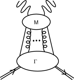
FIG. 1.: Schematic diagram for Compton scattering in terms of quark and gluon scattering amplitudes $M$ and their correlation functions $\Gamma$ in the nucleon.

As a first step of factorization, we consider the most general Feynman diagrams consisting of a hard (perturbative) part representing scattering of a set of quarks and gluons with the photon, and a soft (non-perturbative) part representing the Green’s functions of these quarks and gluons in the presence of the nucleon, as shown in Fig. 1. Denote a collection of incoming (with respect to the hard scattering) quark momenta by $\{p_{i}\}$, outgoing quark momenta by $\{p_{j}^{\prime}\}$ and gluon momenta by $\{k_{\ell}\}$. The quark and gluon scattering amplitude can be expressed as

$$M^{\mu\nu}(q,\{p_{i}\},\{p_{j}^{\prime}\},\{k_{\ell}\})$$ (18)

$$\qquad=i\int e^{iq\cdot\xi}d^{4}\xi\left\langle 0\left|{\cal T}\left\{J^{\mu}(\xi)J^{\nu}(0)\cdots\psi(p_{i})\cdots\bar{\psi}(p_{j}^{\prime})\cdots A(k_{\ell})\cdots\right\}\right|0\right\rangle_{\rm amp}\ ,$$ (19)

where the subscript ‘amp’ indicates that the external quark and gluon legs are truncated and the Lorentz and Dirac indices on gluon and quark fields are left open. The quark and gluon Green’s function in the presence of the nucleon is

$$\Gamma(\{p_{i}\},\{p_{j}^{\prime}\},\{k_{\ell}\})=\left\langle PS\left|{\cal T}\left\{\cdots\bar{\psi}(p_{i})\cdots\psi(p_{j}^{\prime})\cdots A(k_{\ell})\cdots\right\}\right|P\right\rangle\ .$$ (20)

Therefore, the full Compton amplitudes can be written as

$$T^{\mu\nu}(q,p)=\sum_{\rm all~{}diagrams}\int\prod_{ijl}d^{4}p_{i}d^{4}p_{j^{\prime}}d^{4}k_{\ell}M^{\mu\nu}\left(q,\{p_{i}\},\{p_{j}^{\prime}\},\{k_{\ell}\}\right)\otimes\Gamma\left(\{p_{i}\},\{p_{j}^{\prime}\},\{k_{\ell}\}\right)\ ,$$ (21)

where the coupling of Lorentz and color indices between $M^{\mu\nu}$ and $\Gamma$ is implied. For simplicity, we work with bare (unrenormalized) fields and couplings until the end of the calculation.

The contributions to $T^{\mu\nu}$ can be classified in terms of powers of $1/Q$ (loosely speaking, a twist-expansion). Unfortunately, however, $1/Q$ power counting is not simply dimensional counting. Conceptually, it is easy to understand because the transverse momentum of a parton, for instance, is less important than its longitudinal momentum in a hard scattering. We must take these relevant facts into account systematically through a new power counting scheme. To facilitate this counting, we make a collinear expansion of the “hard amplitude” $M^{\mu\nu}(q,\{p_{i}\},\{p_{j}^{\prime}\},\{k_{\ell}\})$ by writing

$$p_{i}^{\mu} = x_{i}p^{\mu}+\Delta p_{i}^{\mu}\;\;,$$ (22)

$$p_{j}^{\prime}\,{}^{\mu} = x_{j}^{\prime}p^{\mu}+\Delta p_{j}^{\prime}\,{}^{\mu}\;\;,$$ (23)

$$k_{\ell}^{\mu} = y_{\ell}p^{\mu}+\Delta k_{\ell}^{\mu}\;\;,$$ (24)

where $x_{i}=p_{i}\cdot n$, and similarly for $p_{j}^{\prime}$ and $k_{\ell}$. Expanding all quark and gluon momenta about the collinear point $\Delta p_{i}^{\mu}=\Delta p_{j}^{\prime}\,{}^{\mu}=\Delta k_{\ell}^{\mu}=0$, we obtain

$$M^{\mu\nu}(q,\{p_{i}\},\{p_{j}^{\prime}\},\{k_{\ell}\})=\sum_{\{m_{i}\},\{n_{j}^{\prime}\},\{t_{\ell}\}}{1\over\cdots m_{i}!\cdots n_{j}^{\prime}!\cdots t_{\ell}!\cdots}$$ (25)

$$\qquad[\cdots(\Delta p_{i})^{m_{i}}\cdots(\Delta p_{j}^{\prime})^{n_{j}^{\prime}}\cdots(\Delta k_{\ell})^{t_{\ell}}\cdots][\cdots\partial\cdots]M^{\mu\nu}(q,\{x_{i}p\},\{x_{j}^{\prime}p\},\{y_{\ell}p\})\;\;,$$ (26)

where we have omitted all the Lorentz indices which couple the partial derivatives with $\Delta p_{i}$, $\Delta p_{i}^{\prime}$, and $\Delta k_{\ell}$. The leading term in the expansion can be interpreted as Compton scattering off of several collinear onshell partons with Feynman momentum fractions $x_{i}=n\cdot p_{i}$, etc. Higher order terms take offshellness and non-collinear effects into account perturbatively.

Rewriting all the quark and gluon momentum integrals in Eq. (21) in terms of these variables, we can integrate out $\Delta p_{i}$, etc. Then the $\Delta$-factors in Eq. (26) become spatial derivatives on the quark and gluon fields in $\Gamma(\{p_{i}\},\{p_{j}^{\prime}\},\{k_{\ell}\})$, which leads to

$$T^{\mu\nu}(q,p) = \sum_{\rm all~{}diag.}\sum_{\{m_{i}\},\{n_{j}^{\prime}\},\{t_{\ell}\}}{1\over\cdots m_{i}!\cdots n_{j^{\prime}}!\cdots t_{\ell}!\cdots}$$ (28)

$$\prod_{ijk}\int dx_{i}dx_{j}^{\prime}dy_{\ell}(\cdots\partial\cdots)M^{\mu\nu}(q,p,\{x_{i}\},\{x_{j}^{\prime}\},\{y_{\ell}\})\Gamma_{mnt}(\{x_{i}\},\{x_{j}^{\prime}\},\{y_{\ell}\})\;\;.$$

The new correlations $\Gamma_{mnt}$ have field separations restricted to the light-cone $n^{\mu}$-direction in the coordinate space, and hence are called light-cone correlations:

$$\Gamma_{mnt}(\{x_{i}\},\{x_{j}^{\prime}\},\{y_{\ell}\})=\prod_{ij\ell}\int{d\lambda_{i}\over 2\pi}{d\mu_{j}\over 2\pi}{d\nu_{\ell}\over 2\pi}e^{i(\lambda_{i}x_{i}+\mu_{j}x_{j}^{\prime}+y_{\ell}\nu_{\ell})}$$ (29)

$$\qquad\qquad\times\langle PS|\cdots\partial^{m_{i}}\bar{\psi}(\lambda_{i}n)\cdots\partial^{n_{j}}\psi(\mu_{j}n)\cdots\partial^{t_{\ell}}A(\nu_{\ell}n)\cdots|PS\rangle\;\;,$$ (30)

where again we have omitted the Lorentz and color indices.

Now, we are ready to introduce light-cone power counting. The hard part in Eq. (28) contains only two momenta, $q^{\mu}$ and $p^{\mu}$, and the only dimensionful scalar in the absence of quark mass effects is $Q^{2}$. [The effects of finite quark mass can be taken into account systematically, as explained in Subsection 3E.] On the other hand, the soft part depends on the scale $\Lambda_{\rm QCD}$. Because there are Lorentz indices that couple the soft and hard parts, $1/Q$ power counting is not determined entirely by the dimension counting of the soft and hard part alone. Instead we need a new type of power counting: light-cone power counting. Since the $T^{\mu\nu}$ has a fixed dimension, we can figure out $1/Q$ counting by studying behavior of either the hard or the soft part. Here we choose to examine the soft part.

The light-cone correlation functions in the collinear expansion involve QCD fields and their derivatives. Lorentz covariance requires that these objects be expressed in terms of $p^{\mu}$, $n^{\mu}$, $g^{\mu\nu}_{\perp}\equiv g^{\mu\nu}-p^{\mu}n^{\nu}-p^{\nu}n^{\mu}$, $\epsilon^{\mu\nu}_{\perp}\equiv\epsilon^{\mu\nu\alpha\beta}p_{\alpha}n_{\beta}$, and $S_{\perp}^{\mu}$. Different $1/Q$ powers result when these vectors are contracted with the hard partonic scattering amplitudes. Note that the contractions of Lorentz structures never produce any soft dimension because of the choice of the collinear coordinates. The balancing soft dimension in each term comes from the scalar coefficients of the expansion, taking into account $[p]=1$, $[n]=-1$ and $[g]=[\epsilon]=[S_{\perp}]=0$. Because the dimension of the Compton amplitude is fixed, the soft dimensions of the scalar coefficients determine the associated hard dimensions. Obviously, the terms with the lowest soft dimension dominate the contribution.

For example, if the soft and hard parts are connected by two-quark lines, we have the following light-cone correlation function :

$$\int{d\lambda\over 2\pi}\,e^{i\lambda x}\langle PS|\bar{\psi}_{\alpha}(0)\psi_{\beta}(\lambda n)|PS\rangle=2\left[\gamma^{\mu}_{\beta\alpha}p_{\mu}q(x)+\gamma^{\mu}_{\beta\alpha}n_{\mu}f_{4}(x)+\cdots\right]$$ (31)

By dimensional counting, $[q(x)]=0$ and $[f_{4}(x)]=2$. Therefore, the $q(x)$ contribution to the hard scattering is leading and the $f_{4}(x)$ contribution is suppressed by a factor of $1/Q^{2}$ relative to $q(x)$.

The relation between counting the soft dimension and the use of the infinite-momentum frame is now easy to see. Since $p^{\mu}\sim\Lambda$, the contribution of the associated term is leading in the limit of $\Lambda\rightarrow\infty$. On the other hand, $n^{\mu}\sim\Lambda^{-1}$, so contributions associated with this vector are doubly suppressed. The Lorentz structures spanning transverse dimensions are ${\cal O}(\Lambda^{0})$ as $\Lambda\rightarrow\infty$. Hence, their contributions are suppresed relative to the $p^{\mu}$ terms, but enhanced related to the $n^{\mu}$ type.

This fact allows us to separately identify a certain power suppression for each field and derivative in the correlation function. For gluon fields, one has

$$A^{+}\sim(1/Q)^{0}\;\;,\qquad A_{\perp}\sim(1/Q)^{1}\;\;,\qquad A^{-}\sim(1/Q)^{2}\;\;\ .$$ (32)

As required by the form of the covariant derivative, partial derivatives obey the same counting rules as gauge fields. Now, we see why our power counting arguments cannot be made until after the collinear expansion : subleading momentum components alter the form of the correlation functions, leading to an extra suppression. Until this behavior is made explicit, our correlation functions do not have a definite power counting. An analysis of the quark bilinears, taking into account the fact that fermion fields have mass dimension 3/2, leads to

$$\overline{\psi}\gamma^{+}(1,\gamma_{5})\psi\sim(1/Q)^{2}\;\;,\qquad\overline{\psi}\gamma^{\perp}(1,\gamma_{5})\psi\sim(1/Q)^{3}\;\;,\qquad\overline{\psi}\gamma^{-}(1,\gamma_{5})\psi\sim(1/Q)^{4}\;\;,$$ (33)

$$\overline{\psi}(1,\gamma_{5})\psi\sim(1/Q)^{3}\;\;,\qquad\qquad\overline{\psi}\sigma^{+-}\psi\sim(1/Q)^{3}\;\;,\qquad\qquad\overline{\psi}\sigma^{\perp\perp^{\prime}}\psi\sim(1/Q)^{3}\;\;,\qquad$$ (34)

where $\gamma^{\pm}=(\gamma^{0}\pm\gamma^{3})/\sqrt{2}$ and $(1,\gamma_{5})$ means either 1 or $\gamma_{5}$. These relations can be simplified by breaking the quark field into two parts :

$$\psi=\psi_{+}+\psi_{-}\;\;,\qquad\psi_{\pm}={1\over 2}\gamma^{\mp}\gamma^{\pm}\psi\;\;,$$ (35)

and writing simply

$$\psi_{+}\sim(1/Q)^{1}\;\;,\qquad\psi_{-}\sim(1/Q)^{2}\;\;.$$ (36)

The suppression associated with an arbitrary correlation function is simply the sum of the suppressions associated with its constituent fields and derivatives minus two for the external nucleon states.

A general light-cone correlation $\Gamma$ is the nucleon matrix element of an operator with $n_{\phi}$ $\phi$ fields, for $\phi=A^{+},A^{\perp},A^{-},\psi_{+},\psi_{-}$, and $n_{\theta}$ partial derivatives, for $\theta=\partial_{\perp},\partial^{-}$. According to the above discussion, its soft dimension is given by

$$n_{\partial_{\perp}}+n_{A_{\perp}}+n_{\psi_{+}}+2(n_{\partial^{-}}+n_{A^{-}}+n_{\psi_{-}})+0\cdot n_{A^{+}}-2\;\;.$$ (37)

Armed with this formula, we can immediately determine the order at which a particular correlation function enters our amplitudes. For instance, the leading contribution to DIS comes from correlations with either two $\psi_{+}$ or two $A_{\perp}$ correlations with arbitrary number of $A_{+}$.

For polarized DIS with transverse polarization, the leading contribution is of order $1/Q$. The possible field combinations at this order are $\bar{\psi}_{\mp}\psi_{\pm}$, $A_{-}A_{\perp}$, $A_{\perp}A_{\perp}A_{\perp}$, $\psi_{+}A_{\perp}\psi_{+}$, $\psi_{+}\partial_{\perp}\psi_{+}$ and $A_{\perp}\partial_{\perp}A_{\perp}$, each appearing with an arbitrary number of $A^{+}$’s. For each of these correlations, we need to consider all possible Feynman diagrams with corresponding external legs. The momenta entering these legs are all collinear.

B Longitudinal Gluons, Gauge Invariance and the Light-Cone Gauge

As we have seen in the last subsection, the longitudinal gauge potential, $A^{+}$, in light-cone correlations does not lead to any suppression in its contribution to scattering amplitudes. At any given order in $1/Q$, an infinite set of correlations with increasing number of $A^{+}$’s contribute. A related problem is that of gauge-invariance. The correlations that naturally appear in the collinear expansion are not manifestly gauge invariant. In particular, the spatially separated fields do not form gauge-invariant operators without appropriate gauge links. The appearance of gauge potentials also poses a gauge-invariance problem since these objects do no transform covariantly under the action of the gauge group. As we have mentioned before, the parton scattering amplitudes $M^{\mu\nu}$ are calculated with external collinear and on-shell parton states after collinear expansion. As such, they are separately gauge invariant. Since the Compton amplitudes are gauge invariant order by order in $1/Q$, all correlations at a given order must combine in such way to yield gauge invariant parton distributions. Gluon potentials and partial derivatives do not transform covariantly under the gauge group, so they must combine to form either covariant derivatives or field strength tensors.

In this subsection, we argue that the infinite number of correlations must be combined into a finite number of gauge-invariant parton distributions. In particular, the correlations with increasing numbers of $A^{+}$’s form gauge-invariant structures with gauge links connecting fields at separate spacetime points. This conclusion is, of course, well-known in the case of leading twist [8]. We assert that it is in fact true order by order in $1/Q$.

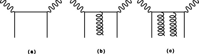
FIG. 2.: A set of tree-level twist-two contributions to DIS, differing in the number of longitudinal gluons participating in hard scattering.

Let us recall the argument of gauge-link formation in the leading twist case. Consider a class of diagrams with a number of $A^{+}$ gluons connecting the soft and hard parts. As we stated above, the hard part is already gauge invariant and can be calculated in any gauge one likes. Using Ward identities derived from the gauge symmetry, one factorizes all the longitudinal gluon lines connected to the hard scattering blob onto eikonal lines. These eikonal lines represent the gauge links. To prove this fact, one refers to the proof of factorization by Collins, Soper and Sterman in Ref. [1]. At leading order in $1/Q$ and $\alpha_{s}(Q^{2})$, this process is especially easy to see. Collecting the contributions from the diagrams in Fig. 2, one obtains

$$T^{\mu\nu} = ie_{q}^{2}\int\,{dxd\lambda\over 2\pi}\,e^{i\lambda x}\left\langle PS\left|\bar{\psi}_{+}(0)\gamma^{\mu}\right.\right.$$ (42)

$$\qquad\times\left[{i\over x\not\!p+\not\!q}+\int\,{dy_{1}d\mu_{1}\over 2\pi}\,e^{i\mu_{1}y_{1}}\,{i\over(x+y_{1})\not\!p+\not\!q}\left(-igA^{+}(\mu_{1}n)\gamma^{-}\right)\,{i\over x\not\!p+\not\!q}\right.$$

$$\qquad\left.+\int\,{dy_{1}d\mu_{1}\over 2\pi}\,{dy_{2}d\mu_{2}\over 2\pi}\,e^{i\mu_{1}y_{1}+i\mu_{2}y_{2}}\,{i\over(x+y_{1}+y_{2})\not\!p+\not\!q}\left(-igA^{+}(\mu_{2}n)\gamma^{-}\right)\,\right.$$

$$\qquad\qquad\times\left.{i\over(x+y_{1})\not\!p+\not\!q}\left(-igA^{+}(\mu_{1}n)\gamma^{-}\right)\,{i\over x\not\!p+\not\!q}+\cdots\right]\left.\left.\gamma^{\nu}\psi_{+}(\lambda n)\right|PS\right\rangle\;\;$$

$$\qquad\qquad\qquad\qquad\qquad\qquad+(\mu\leftrightarrow\nu,q\rightarrow-q)\;\;.$$

For illustrative purposes, we take $\mu\nu$ in the transverse dimensions and simplify the Dirac algebra. Giving $x_{B}=Q^{2}/2p\cdot q$ a small negative imaginary part and performing the integrals over the $y_{i}$, we obtain

$$T^{\mu\nu} = -{e_{q}^{2}\over 2}\int{dxd\lambda\over 2\pi}\;{1\over x-x_{B}}\;e^{i\lambda x}\left\langle PS\left|\bar{\psi}(0)\gamma^{\mu}\not\!n\right.\right.$$ (45)

$$\times\left[1+\int_{\lambda}^{0}d\mu_{1}\,(-igA^{+}(\mu_{1}n))+\int_{\lambda}^{0}d\mu_{1}\,(-igA^{+}(\mu_{1}n))\int_{\lambda}^{\mu_{1}}d\mu_{2}\,(-igA^{+}(\mu_{2}n))+\cdots\right]$$

$$\qquad\qquad\qquad\times\left.\left.\gamma^{\nu}\psi(\lambda n)\right|PS\right\rangle\;\;+\;\;(\mu\leftrightarrow\nu,q\rightarrow-q)\;\;.$$

The quantity in brackets is precisely the gauge link required to make this distribution gauge-invariant.

At higher orders in the $1/Q$ expansion, we have more fields and this process of resummation becomes more complicated. However, at any given order in $1/Q$, there is only a finite number of $A_{\perp}$ and $A^{-}$ according to power counting. These potentials require only a finite number of $A^{+}$’s and partial derivatives to form gauge covariant quantities. Therefore the infinite number of remaining $A^{+}$’s must form gauge-covariant objects by themselves. One can easily see by inspection that this can only be achieved if they form gauge links. Once done, we are left with a finite number of correlations with gauge links.

After an infinite number of longitudinal gluons have been resummed to form the gauge links, the remainder must combine with the partial derivatives and the $A_{\perp}$ and $A^{-}$ fields to form fully gauge-invariant distributions. This means that they must organize into covariant derivatives and field strength tensors. Although difficult to prove, this fact is a direct consequence of gauge invariance. It can be used as a check of any explicit calculation.

In a practical calculation, the presence of the longitudinal gluons represents an unncessary complication. The standard approach to avoiding this is to make the choice of light-cone gauge $A^{+}=0$. Although a gauge choice here is not required since we are not making perturbative calculations of the correlations, it represents a tremendous simplification. In this gauge, no correlations involving $A^{+}$ are ever needed and the gauge links simply reduce to unity. The only complication comes at the end of the calculation, when we would like to organize the correlations in the axial gauge into manifestly gauge invariant ones.

As a last point in this subsection, we mention that not all the correlations that one can write down according to the light-cone power counting above are independent. The so-called ‘bad’ field components, $\psi_{-}$ and $A^{-}$, are related to the ‘good’ components, $\psi_{+}$ and $A_{\perp}$, through the QCD equations of motion:

$$\not\!n\;\not\!\!\!\!iD\psi=\not\!n\!\not\!p\,iD^{+}\psi+\not\!n\;\not\!\!\!\!iD_{\perp}\psi=2iD^{+}\psi_{-}+\not\!n\;\not\!\!\!\!iD_{\perp}\psi_{+}=0\;\;,$$ (46)

where we have introduced the covariant derivative

$$D_{\alpha}(\mu n)\equiv\partial_{\alpha}+igA_{\alpha}(\mu n)\;\;.$$ (47)

In the light-cone gauge, we can solve this equation for the ‘bad’ quark field component in terms of the ‘good’ one:

$$\psi_{-}(\lambda n)={i\over 2}\int^{\lambda}\,d\zeta\not\!n\;\not\!\!\!\!iD_{\perp}(\zeta n)\psi_{+}(\zeta n)\;\;.$$ (48)

Similarly, one has

$$A_{a}^{-}(\lambda n)=-\int^{\lambda}\,d\zeta\,\int^{\zeta}\,d\zeta^{\prime}\left[D^{ab}_{\perp}(\zeta^{\prime}n)\partial^{+}A_{b}^{\perp}(\zeta^{\prime}n)+g\overline{\psi}_{+}(\zeta^{\prime}n)\not\!n\,t^{a}\psi_{+}(\zeta^{\prime}n)\right]\ .$$ (49)

from the gluon equation of motion. The above equations are consistent with the light-cone power counting of the previous subsection. In both cases, we see that the ‘bad’ components, $\psi_{-}$ and $A^{-}$, can be eliminated in favor of either two ‘good’ fields, $\psi_{+}$ or $A_{\perp}$, or one ‘good’ field and a transverse momentum insertion. This follows from the fact that in light-cone quantization, ‘bad’ field components do not propagate freely and hence cannot be directly interpreted in Feynman-Dyson type perturbation theory. As a consequence, we can choose independent correlations without inclusion of any “bad” fields.

C Example: $S_{T}$ in the Leading Order

As an example of formalism presented above, we consider the leading contribution to $S_{T}(\nu,Q^{2})$. This example is useful not only as a simple illustration of the procedure, but also to familiarize the reader with some of the distributions that appear in DIS with transverse polarization. To simplify the discussion, we contract one of the photon polarizations with $n^{\mu}$. This leads to

$$T^{[\mu+]}=i\epsilon^{-+\beta\mu}\,{MS_{\beta}\over\nu}\,x_{B}\,S_{T}(\nu,Q^{2})\;\;,$$ (50)

where $\mu$ is transverse.

In the light-cone gauge, there are two independent correlations at leading order in $\alpha_{s}(Q^{2})$. The first involves the good components of two quark fields and a transverse partial derivative:

$$\Gamma_{qqB}^{\alpha}(x,y) = \int{d\lambda\over 2\pi}{d\mu\over 2\pi}e^{i\lambda x}e^{i\mu(y-x)}\langle PS|\bar{\psi}_{+}(0)i\partial^{\alpha}_{\perp}\psi_{+}(\lambda n)|PS\rangle$$ (51)

$$= \delta(x-y)\int{d\lambda\over 2\pi}e^{i\lambda x}\langle PS|\bar{\psi}_{+}(0)i\partial^{\alpha}_{\perp}\psi_{+}(\lambda n)|PS\rangle\ ,$$ (52)

where the Dirac and color indices on quark fields are open and $\alpha$ is transverse. The second correlation contains two quark and one gluon field :

$$\Gamma_{qgqB}^{\alpha}(x,y)=\int{d\lambda\over 2\pi}{d\mu\over 2\pi}e^{i\lambda x}e^{i\mu(y-x)}\langle PS|\bar{\psi}_{+}(0)(-g_{B})A^{\alpha}_{\perp}(\mu n)\psi_{+}(\lambda n)|PS\rangle\ .$$ (53)

The leading-order result for $S_{T}(\nu,Q^{2})$ must be expressible in terms of these correlations alone.

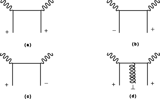
FIG. 3.: Tree-level Feynman diagrams for $S_{T}$. The pluses (+) and minuses (-) refer to the light-cone projections of the Dirac fields.

The tree level Feynman diagrams for $M^{\mu+}$ are shown in Fig. 3. The total contributions to $T^{\mu+}$ can be expressed as

$$T^{[\mu+]}= {e_{q}^{2}\over 2\nu}\int\,dx\,dy\int\,{d\lambda\over 2\pi}\,{d\mu\over 2\pi}\,e^{i\lambda x}\,e^{i\mu(y-x)}$$ (57)

$$\times\,\left\langle PS\left|\overline{\psi}_{+}(0)\left[{1\over y-x_{B}}\,\gamma^{\mu}\not\!n\;\not\!\!\!\!iD_{\perp}(\mu n)-{1\over x+x_{B}}\;\not\!\!\!\!iD_{\perp}(\mu n)\not\!n\gamma^{\mu}\right]\,\psi_{+}(\lambda n)\right|PS\right\rangle$$

$$-{e_{q}^{2}\over 2\nu}\int\,dx\int{d\lambda\over 2\pi}\,e^{i\lambda x}\left\langle PS\left|\overline{\psi}_{-}(0)\not\!p\not\!n\gamma^{\mu}\psi_{+}(\lambda n)\right|PS\right\rangle$$

$$+{e_{q}^{2}\over 2\nu}\int\,dx\int{d\lambda\over 2\pi}\,e^{i\lambda x}\left\langle PS\left|\overline{\psi}_{+}(0)\gamma^{\mu}\not\!n\not\!p\,\psi_{-}(\lambda n)\right|PS\right\rangle\;\;.$$

The special form of the kernels in contribution (57) allows us to “simplify” this contribution using the equation of motion. It then combines with the others to give the full result

$$T^{[\mu+]} = i\epsilon^{\mu+-\alpha}(-x_{B})\,{e_{q}^{2}\over 2\nu}\,\int\,dx\,\left({1\over x-x_{B}}-{1\over x+x_{B}}\right)$$ (59)

$$\qquad\times\int\,{d\lambda\over 2\pi}e^{i\lambda x}\,\left\langle PS\left|\overline{\psi}(0)\gamma_{\alpha}\gamma_{5}\psi(\lambda n)\right|PS\right\rangle\;\;.$$

As a consequence of parity and time-reversal invariance, one can isolate a scalar distribution,

$$\int{d\lambda\over 4\pi}\,e^{i\lambda x}\,\left\langle PS\left|\overline{\psi}(0)\gamma_{\alpha}\gamma_{5}\psi(\lambda n)\right|PS\right\rangle=(MS)_{\alpha}\,q_{TB}(x)\;\;,$$ (60)

and write

$$S^{(0)}_{T}(\nu,Q^{2})=-\sum_{q}e_{q}^{2}\int\,dx\left({1\over x-x_{B}}-{1\over x+x_{B}}\right)q_{TB}(x)\;\;$$ (61)

at leading order in the strong coupling. Recall that this distribution, as it appears here, is not renormalized. However, since the difference appears only at higher orders in $\alpha_{s}(Q^{2})$, we can replace it with a renormalized distribution $q_{T}(x,Q^{2})$. [Note that $q_{T}(x,Q^{2})$ can be made manifestly gauge-invariant by re-introducing the $A^{+}$ fields in the form of a light-cone gauge link connecting the quark fields.]

It is now a simple matter to determine the scaling function $g_{T}(x_{B},Q^{2})$ in terms of $q_{T}(x,Q^{2})$ :

$$g^{(0)}_{T}(x_{B},Q^{2})={1\over 2}\sum_{q}\,e_{q}^{2}\,\left[q_{T}(x_{B},Q^{2})+q_{T}(-x_{B},Q^{2})\right]\;\;.$$ (62)

This extremely simple result is quite misleading. It seems to imply that only one function of a single variable is required to predict the ${\cal O}(1/Q)$ corrections to DIS. In analogy with the leading ${\cal O}(1)$ result, one might assume that higher order corrections will do nothing but modify the form of the coefficient function. Furthermore, one might expect that the $Q^{2}$ variation of this new distribution is fixed from the distribution itself. Unfortunately, neither of these suspicions is correct. The fact that our leading result can be expressed so simply in terms of $q_{T}(x,Q^{2})$ is due exclusively to the form of the coefficient function in contribution (57). There is no reason to believe that this simple form will persist at higher orders.

To reveal the full content of $g_{T}(x_{B},Q^{2})$ at this order, we use the equation of motion to eliminate the “bad” fields. The result can be expressed in terms of the single gauge-invariant correlation

$$K_{qB}^{\alpha}(x,y) = \Gamma^{\alpha}_{qqB}(x,y)+\Gamma^{\alpha}_{qgqB}(x,y)$$ (63)

$$= \int{d\lambda\over 2\pi}{d\mu\over 2\pi}e^{i\lambda x}e^{i\mu(y-x)}\langle PS|\bar{\psi}(0)iD^{\alpha}_{\perp}(\mu n)\psi(\lambda n)|PS\rangle\ ,$$ (64)

where color indices have been contracted but the Lorentz indices are open. The only invariant correlation $K_{qB}(x,y)$ appears in the contraction

$$\int\,{d\lambda\over 4\pi}\,{d\mu\over 4\pi}\,e^{i\lambda x}\,e^{i\mu(y-x)}\,\left\langle PS\left|\overline{\psi}(0)\;\not\!\!\!\!iD_{\perp}(\mu n)\not\!n\gamma^{\mu}\psi(\lambda n)\right|PS\right\rangle=\phantom{-}i\epsilon^{-+\alpha\mu}MS_{\alpha}K_{qB}(x,y)\;\;,$$ (65)

$$\int\,{d\lambda\over 4\pi}\,{d\mu\over 4\pi}\,e^{i\lambda x}\,e^{i\mu(y-x)}\,\left\langle PS\left|\overline{\psi}(0)\gamma^{\mu}\not\!n\;\not\!\!\!\!iD_{\perp}(\mu n)\psi(\lambda n)\right|PS\right\rangle=-i\epsilon^{-+\alpha\mu}MS_{\alpha}K_{qB}(y,x)\;\;,$$ (66)

of these latter indices. Since

$$\int\,{d\lambda\over 4\pi}\,{d\mu\over 4\pi}\,e^{i\lambda x}\,e^{i\mu(y-x)}\,\left\langle PS\left|\overline{\psi}(0)(-ig)F^{+\alpha}(\mu n)\gamma_{\alpha}\not\!n\gamma^{\mu}\psi(\lambda n)\right|PS\right\rangle$$ (67)

$$\qquad\qquad\qquad\qquad=i\epsilon^{-+\alpha\mu}MS_{\alpha}(y-x)K_{qB}(x,y)\;\;,$$ (68)

every gauge-invariant way to include two ‘good’ quark fields and either a ‘good’ gluon field or a transverse partial derivative can be accomodated by $K_{qB}(x,y)$. Furthermore, the first moment of $K_{qB}(x,y)$ with respect to $y$ generates the ‘bad’ component of the quark field through the equation of motion. Hence all of the distributions relevant to ${\cal O}(1/Q)$ DIS are contained in $K_{qB}(x,y)$. This fact allows us to assert that all ${\cal O}(1/Q)$ corrections to DIS in the nonsinglet sector can be expressed in terms of $K_{qB}(x,y)$. In the singlet sector, one must introduce one more distribution to describe pure gluonic effects. This is done in Section 4.

In terms of $K_{qB}(x,y)$, our leading correction has the form

$$S^{(0)}_{T}(\nu,Q^{2})=-\sum_{q}e_{q}^{2}\int\,dx\,dy\,{2\over x}\left({1\over x-x_{B}}-{1\over x+x_{B}}\right)\,K_{q}(x,y,Q^{2})\;\;,$$ (69)

where we have once again ignored the difference between renormalized and unrenormalized distributions. In the remainder of this paper, we will be concerned with determining the ${\cal O}(\alpha_{s})$ corrections to this result.

D Factorization of Infrared Singularities and Radiative Corrections

Up to this point, we haven’t said much about the perturbative coefficients $M^{\mu\nu}$ of the correlation functions other than that they are calculated in terms of collinear and on-shell external parton states and that they are gauge invariant. They are, of course, perturbative expansions in the strong coupling, $\alpha_{s}(Q^{2})$. Hence, the final result for $T^{\mu\nu}$ is a double expansion. As $Q$ becomes large, both expansion parameters vanish. Loosely speaking, the $1/Q$ expansion is associated with the number of fields in the soft part of the process, while the coupling expansion is associated with those in the hard part. In this subsection, we would like to elucidate the nature of the latter expansion.

Because the partons are on-shell, $M^{\mu\nu}_{i}$ can be viewed as a parton scattering S-matrix element. In principle, one must multiply by parton wave function renormalization factors to get the proper S-matrix element. However, working in $d=4-\epsilon$ dimensions, the absence of a physical scale at the massless poles of the quark and gluon propagators reduces these contributions to unity. Subleading terms in the expansion of $M^{\mu\nu}_{i}$ are parton scattering S-matrix elements with insertions of certain vertices associated with powers of $k_{j}^{\perp}$ and $k^{-}_{j}(\equiv p\cdot k_{j})$. For instance, with one power of quark momentum $k_{j}^{\perp}$, the subleading term is calculated with one insertion of the vector vertex $i\gamma^{\alpha}_{\perp}$ to one of the quark propagators. Because S-matrix elements and their relatives are gauge invariant, one may choose any gauge for the internal gluon propagators in $M^{\mu\nu}_{i}$. We use Feynman’s choice in our calculation.

As we have argued above, $M_{i}^{\mu\nu}$ is ultraviolet finite because the on-shell wave function renormalization is trivial in dimensional regularization. Nevertheless, due to the massless on-shell external states, $M_{i}^{\mu\nu}$ has infrared divergences showing up as $1/\epsilon$ poles. To understand the origin of the infrared divergences, we consider a vertex correction to the tree-level Compton scattering diagram. Let the gluon momentum be $k$ and one of the quark propagators $k+xp$. Then the loop integral is divergent when $k$ is parallel to $xp$. Using dimensional regularization, this collinear divergence appears as $1/\epsilon$ pole. These divergences may be factorized in the perturbative sense

$$M^{\mu\nu}_{i}=C^{\mu\nu}_{i}\otimes P_{i}\ ,$$ (70)

where $C_{i}^{\mu\nu}$ is the finite coefficient function and $P_{i}$ contains only the $1/\epsilon$ poles. On the other hand, the infrared-finite quantities $\Gamma_{iB}$ contain ultraviolet divergences which also show up as $1/\epsilon$ poles. When the infrared poles in $P_{i}$ cancel all the ultraviolet poles in $\Gamma_{iB}$, $T^{\mu\nu}$ is said to be factorizable. The product $P_{i}\Gamma_{iB}$ defines the renormalized parton correlation functions $\Gamma_{i}$. The final factorization formula for the Compton amplitude is then

$$T^{\mu\nu}=\sum_{i}C^{\mu\nu}_{i}\otimes\Gamma_{i}\ ,$$ (71)

where $C^{\mu\nu}_{i}$ is a well-defined perturbation series in $\alpha_{s}$ and $\Gamma_{i}$ is a finite nonperturbative distribution.

The Feynman diagrams in the hard part are simpler to evaluate after the collinear expansion because all the external momenta become collinear ($p$ and $q$). The only transverse momentum components come from the loop momenta. Therefore, it is convenient to introduce the light-cone coordinates

$$k^{\pm}={1\over\sqrt{2}}(k^{0}\pm k^{3});~{}~{}~{}k_{\perp}=(k^{1},k^{2})\ .$$ (72)

The momentum-integral now becomes $d^{4}k=dk^{+}dk^{-}d^{2}k_{\perp}$. The $dk^{-}$ integral can be done using the residue theorem by considering the complex plane of $k^{-}$. After this is done, the transverse $k_{\perp}$ integrals become straightforward. The remaining $k^{+}$ integral is, in general, a nontrivial multidimensional integral containing both the evolution kernels $P_{i}$ and the finite coefficient functions $C_{i}^{\mu\nu}$. Although this integral can be quite complicated, its dependence on $\epsilon$ has been made explicit by performing the transverse integrals. This allows us to separate the process of verifying factorizability from the calculation of the coefficient functions.

E Summary

We are now in a position to write down a set of rules for calculating the Compton amplitudes at an arbitrary order, $n$, in $1/Q$. First, one must calculate the hard scattering Compton amplitude for every combination of $g$ ‘good’ field components, where $g$ runs from 2 to $n+2$. Only diagrams in which $q^{\mu}$ flows through every loop are considered in this calculation. Initial and final state interactions such as those represented in Fig. 4 are taken into account via renormalization $Z$-factors and the inclusion of the ‘bad’ field components. The external momenta in these amplitudes are written as

$$k_{j}^{\mu}=(k_{j}\cdot n)p^{\mu}+\lambda^{2}(k_{j}\cdot p)n^{\mu}+\lambda k_{j}^{\perp}\;\;,$$ (73)

and the amplitudes are expanded about $\lambda=0$. The coefficient of $\lambda^{n+2-g}$ is convoluted with the correlation function, and factors of $k_{j}^{\perp}$ and $k_{j}^{-}$ are eliminated in favor of partial derivatives acting on fields. Second, one considers processes which involve one ‘bad’ field component and anywhere from one to $n$ ‘good’ field components. The above process is repeated, but here the relevant coefficient comes at order $\lambda^{n+2-g-2}$. Next, amplitudes with two ‘bad’ field components must be considered. This process continues until we have exhausted all possible ways to obtain a suppression of $(\Lambda_{\rm QCD}/Q)^{n}$. In general, one must consider a collinear expansion to order $\lambda^{n+2-g-2b}$ of all amplitudes containing $g$ external ‘good’ field components and $b$ external ‘bad’ field components for which $n+2-g-2b$ is positive or zero.

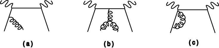
FIG. 4.: Hard scattering diagrams which represent processes that occur either entirely before or after the hard scattering. $(a)$ and $(b)$ are taken care of by the inclusion of ‘bad’ field components along with ‘good’ ones, while the contribution from $(c)$ is grouped into a renormalization $Z$-factor.

As exemplefied by Eqs. (48,49), we could choose to eliminate the ‘bad’ components in the beginning of the calculation. In this scheme, some diagrams representing processes that occur entirely either before or after the hard scattering, such as Figs. 4$(a)$ and $(b)$ (but not $(c)$), are reinstated. Rules for the onshell couplings and propagators that appear in these special diagrams are derived directly from the equations of motion. This procedure is used in Refs. [8, 9]. Throughout the rest of this paper, however, we opt for the former method.

The dependence of $q^{\mu}$ on the nucleon mass $M$ through $\zeta$ (Eqs. (11,14)) prompts us to replace $M\rightarrow\lambda M$ in $\zeta$ before each expansion. This produces additional suppression of certain correlations, but does not significantly alter the above analysis because its effects can always be grouped into the physical vector $q^{\mu}$. If quark mass effects are desired, one has only to replace $\;\not\!\!\!\!iD_{\perp}$ with $\;\not\!\!\!\!iD_{\perp}-m_{q}$ in Eq. (48), consider $m_{q}\rightarrow\lambda m_{q}$ in the amplitudes, and expand as before.

We note here that these expansions may be asymptotic in nature and cannot be used to predict experiment to arbitrary precision because of the problems presented by infrared renormalons [30].

IV One-Loop Corrections to the Transverse Compton amplitude $S_{T}$

Armed with the formalism presented in the last section, we are ready to study the main subject of the paper: one-loop corrections to the $g_{T}$ scaling function. As we have explained before, it is the Compton amplitude $S_{T}$ that is a natural object to calculate in Feynman-Dyson perturbation theory; we focus on it exclusively throughout this section. Part of the results here have already appeared in our previous publications [9, 10]. More details are given here for the reader’s convenience.

A One-Loop Corrections in the Non-Singlet Sector

The non-singlet sector requires at least two quark fields, so the correlation functions we need to consider are exactly the same as those in Section 3C. Before we begin, however, some comments are in order.

As with most quantum loop-corrections, our calculation contains divergences. As explained above Eq. (70), these divergences are of infrared origin after usual renormalization and can be combined with the bare distributions to generate a finite, scale-dependent renormalized distribution. Working in dimensional regularization, one can isolate these divergences and obtain a relation between the renormalized and bare distributions. This relation allows us to determine the $Q^{2}$ evolution of $K_{q}(x,y,Q^{2})$ and check the validity of factorization for our process. Of course, in order to use dimensional regularization to calculate a spin-dependent quantity, one must specify a prescription for $\gamma_{5}$ and $\epsilon^{\mu\nu\alpha\beta}$. In this paper, we choose ‘t Hooft and Veltman’s prescription [31].

In principle, to obtain the full amplitude one must calculate all relevent Feynman diagrams. However, loops associated exclusively with external legs can be grouped into renormalization $Z$-factors for the external fields. The absence of a physical scale at the massless poles of the physical external propagators reduces these factors to unity. In addition, when both photon indices are left open, fundamental symmetries allow one to reduce the number of diagrams that actually need to be calculated. The crossing symmetry, for example, allows one to cut independent diagrams in half by asserting symmetry under the replacement $(\mu\leftrightarrow\nu,q\rightarrow-q)$. In our case, the freedom to exchange $\mu$ and $\nu$ is destroyed by our asymmetric treatment of these indices. However, we know that the part of the amplitude we search for is antisymmetric in $\mu$ and $\nu$, so we can obtain the full result simply by calculating all diagrams with a certain ordering of photon insertions and subtracting $(q\rightarrow-q)$ in the end. Although these diagrams are not all independent when photon indices are left open, they represent the minimal set of independent contributions to our calculation.

By inspection, one can see that there are four diagrams associated with $(g,b)=(2,0)$, sixteen associated with $(3,0)$, and eight with $(1,1)$. These diagrams can easily be grouped according to color factor. All of the diagrams associated with $(2,0)$ and $(1,1)$ are proportional to $C_{F}=(N^{2}-1)/2N$ in SU$(N)$, while those representing $(3,0)$ also include the factors $C_{A}=N$ and $C_{F}-C_{A}/2=-1/2N$. Routing the transverse momentum through the quark line and performing the collinear expansion

$${i\over\not\!\ell+\not\!k_{\perp}}={i\over\not\!\ell}+{i\over\not\!\ell}\;\not\!\!\!ik_{\perp}\,{i\over\not\!\ell}+\cdots$$ (74)

before evaluation, we see that the four (2,0) graphs actually represent twelve contributions, each with an insertion of the operator $\;\not\!\!\!ik_{\perp}\rightarrow i\;\not\!\!\!i\partial_{\perp}$, where the partial derivative acts on the external quark field. Each of these contributions corresponds to a similar graph in which the operator insertion is replaced by a gluon line. The only differences between these contributions are the change in momentum induced by a gluon absorption and the associated gauge group generator. Since the generator contributes only to the color factor, the $(2,0)$ contribution is simply the $C_{F}$-part of the $(3,0)$ contribution evaluated at zero momentum transfer, i.e. $x=y$. This implies that the sum of $(2,0)$ and $(3,0)$ is obtained by replacing $-gA_{\alpha}(\mu n)$ with $iD_{\alpha}(\mu n)$ in the $C_{F}$-part of $(3,0)$. Hence, the $C_{F}$-part of our amplitude is already expressible in terms of $K_{qB}(x,y)$ alone. Since there are no partial derivative terms proportional to $C_{A}$, this part must be gauge-invariant by itself. Looking at Eq. (68), we see that the necessary requirement is that its coefficient vanish at least linearly as $x\rightarrow y$. We will see below that this is in fact the case.

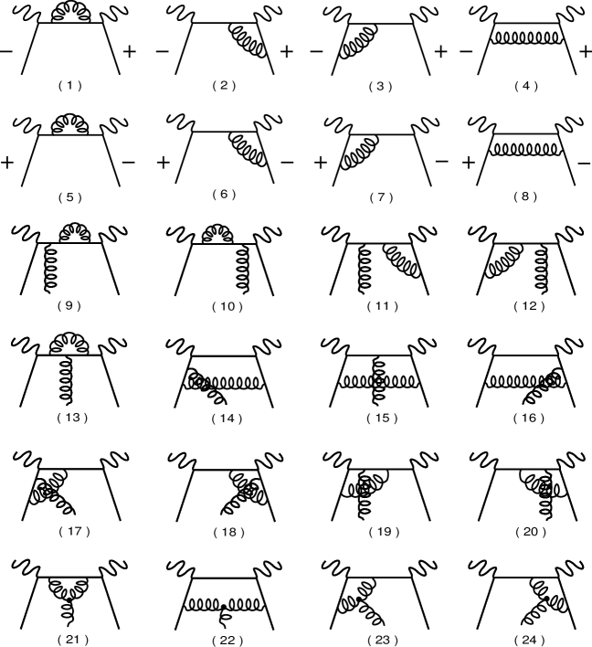
FIG. 5.: Diagrams contributing to the hard scattering coefficient $M^{\mu+}$ relevant to $S_{T}$ at one-loop order in the non-singlet sector. (1)-(12) are proportional to the casimir $C_{F}$, (13)-(20) to $C_{F}-C_{A}/2$, and (21)-(24) to $C_{A}$.

Now that we have successfully reduced the number of diagrams we must calculate from fifty-six (actually, more like seventy-two) to the twenty-four shown in Fig. 5, we are ready to begin the actual calculation. Using the fact that $\not\!n\psi_{-}=\not\!p\psi_{+}=0$ and that none of the external momenta have transverse components, one can reduce every numerator to simple Dirac structures times functions of $k_{\perp}^{2}$, $p\cdot k$, $\nu$, $n\cdot k$, $x$, $y$, and $x_{B}$, where $k^{\mu}$ is the loop-momentum. Using techniques outlined in the Appendix, one can always cancel propagators until there are only three left. At that point, the integrals can easily be done by contour. Useful integration formulae can be found in the Appendix; here, we simply give the result:

$$S_{T}^{NS(1)}(\nu,Q^{2}) = {\alpha_{s}(Q^{2})\over 2\pi}\sum_{q}\hat{e}_{q}^{2}\int\,{dx\,dy\over xy}\,\left[M^{NS}\left({x\over x_{B}},{y\over x_{B}}\right)-(x_{B}\rightarrow-x_{B})\right]\,K_{qB}(x,y)\;\;;$$ (75)

$$M^{NS}(x,y) = C_{F}\left\{{2\over\epsilon}\left({Q^{2}e^{\gamma}\over 4\pi\mu^{2}}\right)^{-\epsilon/2}\left[\vphantom{\left(2y(1-x)\over x^{2}\right)}-{y\over 1-x}\right.\right.$$ (86)

$$\left.\phantom{C_{F}\{}+\left({2y(1-x)\over x^{2}}-{2\over x}-{4y\over 1-x}\right)\log(1-x)-{2\over y}\log(1-y)\right]$$

$$\phantom{C_{F}\{}-{4y\over 1-x}+\left({2y\over x^{2}}+{y-6\over x}+{2-y\over x-y}-{3y\over 1-x}\right)\log(1-x)$$

$$\phantom{C_{F}\{}+\left(3-{6\over y}+{y-2\over x-y}\right)\log(1-y)$$

$$\phantom{C_{F}\{}\left.\vphantom{\left({Q^{2}e^{\gamma}\over 4\pi\mu^{2}}\right)^{-\epsilon/2}}-\left({y(1-x)\over x^{2}}-{1\over x}-{2y\over 1-x}\right)\log^{2}(1-x)+{1\over y}\log^{2}(1-y)\right\}$$

$$-{C_{A}\over 2}\left\{{2\over\epsilon}\left({Q^{2}e^{\gamma}\over 4\pi\mu^{2}}\right)^{-\epsilon/2}\left[{2\over y-x}\log(1-x)+{2\over x-y}\log(1-y)\right]\right.$$

$$\phantom{-{C_{A}\over 2}\{}+{4\over y-x}\log(1-x)+\left({4\over x-y}+{2\over 1-x}\right)\log(1-y)$$

$$\left.\phantom{-{C_{A}\over 2}\{}\vphantom{\left({Q^{2}e^{\gamma}\over 4\pi\mu^{2}}\right)^{-\epsilon/2}}-{1\over y-x}\log^{2}(1-x)-{1\over x-y}\log^{2}(1-y)\right\}$$

$$+\left(C_{F}-{C_{A}\over 2}\right)\left\{{2\over\epsilon}\left({Q^{2}e^{\gamma}\over 4\pi\mu^{2}}\right)^{-\epsilon/2}{2\over x-y}\left({x+y\over x-y}+{xy\over 1-x}\right)\log(1-(x-y))\right.$$

$$\phantom{\left(C_{F}-{C_{A}\over 2}\right)\{}+{2\over x-y}\left(2\,{x+y\over x-y}+{y(3x-1)\over 1-x}\right)\log(1-(x-y))$$

$$\left.\vphantom{\left({Q^{2}e^{\gamma}\over 4\pi\mu^{2}}\right)^{-\epsilon/2}}\phantom{\left(C_{F}-{C_{A}\over 2}\right)\{}-{1\over x-y}\left({x+y\over x-y}+{xy\over 1-x}\right)\log^{2}(1-(x-y))\right\}\;\;,$$

where $\hat{e}_{q}^{2}=e_{q}^{2}-\langle e_{q}^{2}\rangle$ is the nonsinglet part of the quark charge. $\langle e_{q}^{2}\rangle=\sum_{q}e_{q}^{2}/n_{f}$ is the average squared quark charge for $n_{f}$ quarks. We have taken $\mu$ as a reference scale for our regularization procedure, and $\gamma=0.57721\ldots$ is the Euler constant. One can check explicitly that $x-y$ divides the $C_{A}$ part of this expression, as required by gauge invariance.

Interpreting the divergent part of this result as the renormalization of our distribution, we find that

$$\int\,dx\left({1\over x-x_{B}}-{1\over x+x_{B}}\right)\,Q^{2}\,{d\over dQ^{2}}q^{NS}_{T}(x,Q^{2})={\alpha_{s}(Q^{2})\over 2\pi}\,\int\,{dx\,dy\over xy}$$ (87)

$$\qquad\times\left\{C_{F}\left[-{y\over x_{B}-x}+\left({2y(x_{B}-x)\over x^{2}}-2{x_{B}\over x}-{4y\over x_{B}-x}\right)\log\left(1-{x\over x_{B}}\right)\right.\right.$$ (88)

$$\left.\qquad\phantom{\times\{C_{F}[}\qquad\vphantom{\left({2y(x_{B}-x)\over x^{2}}-2{x_{B}\over x}-{4y\over x_{B}-x}\right)}-2{x_{B}\over y}\log\left(1-{y\over x_{B}}\right)\right]$$ (89)

$$\qquad\phantom{\times\{}-{C_{A}\over 2}\left[2{x_{B}\over y-x}\log\left(1-{x\over x_{B}}\right)+2{x_{B}\over x-y}\log\left(1-{y\over x_{B}}\right)\right]$$ (90)

$$\qquad\qquad\phantom{\times\{}+\left(C_{F}-{C_{A}\over 2}\right)\,2{x_{B}\over x-y}\left({x+y\over x-y}+{xy\over x_{B}(x_{B}-x)}\right)\log\left(1-{x-y\over x_{B}}\right)$$ (91)

$$\left.\qquad\qquad\qquad\phantom{\times\{}\vphantom{{2y(1-x)\over x-r}}-(x_{B}\rightarrow-x_{B})\right\}K_{NS}(x,y,Q^{2})\;\;.$$ (92)

From this result, one can immediately see that the evolution of $q^{NS}_{T}(x,Q^{2})$ is not self-contained. This is one of the main reasons Eq. (61) is misleading. The distribution $q^{NS}_{T}(x,Q^{2})$ makes sense by itself only for one value of $Q^{2}$. Once that value is changed, one requires input from the full function $K_{NS}(x,y,Q^{2})$ to define it.

At this point, we can take the imaginary part of Eq. (75) as $x_{B}$ approaches the real axis from below to obtain the next-to-leading expression for $g^{NS}_{T}(x_{B},Q^{2})$. This is done in Ref. [9]. For now, we turn to the singlet sector.

B One-Loop Corrections in the Singlet Sector

At this order in $\alpha_{s}(Q^{2})$, gluons can interact with the photons through a virtual quark loop. This process generates a contribution to $S_{T}$ from purely gluonic effects. Using our power-counting techniques, we see that once again we must consider three different correlations : $(g,b)=(2,0),(3,0)$, and $(1,1)$. As before, the contributions to $(2,0)$ can be obtained from those to $(3,0)$. However, due to the bosonic symmetry of the gauge fields, the symmetries associated with this process are quite different.

Let us consider first the contributions to $(1,1)$. These are represented by a quark loop with two photons, a transverse gluon, and a longitudinal gluon attached. Including the bosonic symmetries for both gluons and photons, a total of six diagrams contribute to this amplitude. Using the properties of fermionic traces, we can reduce this to the three contributions shown in Fig. 6. An explicit calculation shows that these contributions exactly cancel. Since this is the only place where, through Eq. (49), one can generate a purely singlet quark contribution, we see that the singlet quark contribution to $S_{T}^{(1)}$ is identical to the nonsinglet contribution for each quark.

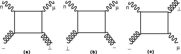
FIG. 6.: Diagrams relevant to $S_{T}$ at one-loop order in the singlet sector involving one ‘bad’ gluon field component. The sum of the three contributions vanishes.

The amplitude associated with $(3,0)$ has twenty-four separate diagramatic contributions once one has taken the three-fold bosonic symmetry into account. Leaving our gluon indices open, we can reduce this number to four. Once again, the properties of the fermion trace allow us to cut this number in half. Hence we are left with only two independent contributions to our amplitude. These contributions are represented by the diagrams in Fig. 7. To obtain the full amplitude, we simply double the charge-conjugation even part of these diagrams and add the gluon permutations. A symmetry factor of $1/6$ must also be applied to associate the amplitude with our correlation function.

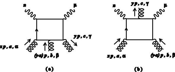
FIG. 7.: The two independent contributions to $M^{\mu+\alpha\beta\gamma\;(g)}_{(3,0)}$.

After simplification, the contributions from Figs. 7 $(a)$ and $(b)$ have the form

$$M^{\mu+\alpha\beta\gamma\;(g)}_{(3,0)a}$$ (93)

$$\quad=\left({i\over 2}T_{F}\,f^{abc}\right)(-g_{B}){\langle e_{q}^{2}\rangle\over\nu}\left[A_{1}(\tilde{x},\tilde{y})g_{\perp}^{\mu\alpha}g_{\perp}^{\beta\gamma}+B_{1}(\tilde{x},\tilde{y})g_{\perp}^{\mu\beta}g_{\perp}^{\gamma\alpha}+C_{1}(\tilde{x},\tilde{y})g_{\perp}^{\mu\gamma}g_{\perp}^{\alpha\beta}\right]\;\;,$$ (94)

$$M^{\mu+\alpha\beta\gamma\;(g)}_{(3,0)b}$$ (95)

$$\quad=\left({i\over 2}T_{F}\,f^{abc}\right)(-g_{B}){\langle e_{q}^{2}\rangle\over\nu}\left[A_{2}(\tilde{x},\tilde{y})g_{\perp}^{\mu\alpha}g_{\perp}^{\beta\gamma}+B_{2}(\tilde{x},\tilde{y})g_{\perp}^{\mu\beta}g_{\perp}^{\gamma\alpha}+C_{2}(\tilde{x},\tilde{y})g_{\perp}^{\mu\gamma}g_{\perp}^{\alpha\beta}\right]\;\;,$$ (96)

respectively, where $f^{abc}$ are the structure constants of the group, $T_{F}=1/2$ is the generator normalization, and $\tilde{x}=x/x_{B}$, $\tilde{y}=y/x_{B}$ represent the relative momentum fractions. Here, we have ignored the C-odd $d^{abc}$ contribution which cannot contribute due to Furry’s theorem. The full amplitude becomes

$$T^{\mu+\;(g)}_{(3,0)} = -{1\over 6}\,T_{F}\,{\langle e_{q}^{2}\rangle\over\nu}\,\int\,dx\,dy\left[f\left({y-x\over x_{B}},-{x\over x_{B}}\right)g_{\perp}^{\mu\alpha}g_{\perp}^{\beta\gamma}\right.$$ (99)

$$\phantom{-{1\over 6}\,T_{F}\,{\langle e_{q}^{2}\rangle\over\nu}\,\int\,dx\,dy}+f\left(-{y\over x_{B}},{x-y\over x_{B}}\right)g_{\perp}^{\mu\beta}g_{\perp}^{\gamma\alpha}$$

$$\phantom{-{1\over 6}\,T_{F}\,{\langle e_{q}^{2}\rangle\over\nu}\,\int\,dx\,dy}\left.+f\left({x\over x_{B}},{y\over x_{B}}\right)g_{\perp}^{\mu\gamma}g_{\perp}^{\alpha\beta}\right]\,(\Gamma_{3gB})_{\gamma\beta\alpha}(x,y)\;\;;$$

$$f(x,y) = \phantom{+}A_{1}(-y,x-y)+A_{2}(-y,x-y)-A_{1}(-y,-x)-A_{2}(-y,-x)$$ (102)

$$+B_{1}(y-x,-x)+B_{2}(y-x,-x)-B_{1}(x,x-y)-B_{2}(x,x-y)$$

$$+C_{1}(x,y)+C_{2}(x,y)-C_{1}(y-x,y)-C_{2}(y-x,y)\;\;,$$

$$(\Gamma_{3gB})_{\alpha\beta\gamma}(x,y) = \int{d\lambda\over 2\pi}\,{d\mu\over 2\pi}\,e^{i\lambda x}\,e^{i\mu(y-x)}\,\left\langle PS\left|(-igf_{abc})A^{a}_{\alpha}(0)A^{b}_{\beta}(\mu n)A^{c}_{\gamma}(\lambda n)\right|PS\right\rangle\;\;,$$ (103)

where we have multiplied by a factor of two to take both possible directions of fermion flow into account and included a factor of six for gluon symmetry. Due to the bosonic symmetry of the gauge fields, all of the terms in Eq. (99) are identical; our result can be rewritten as

$$T^{\mu+\;(g)}=-{1\over 2}\,T_{F}\,{\langle e_{q}^{2}\rangle\over\nu}\int\,dx\,dy\,f\left({x\over x_{B}},{y\over x_{B}}\right)\,(\Gamma_{3gB})^{\mu\alpha}_{\;\;\alpha}(x,y)\;\;.$$ (104)

This amplitude must combine with that associated with $(2,0)$ to make a fully gauge invariant contribution to $S^{(1)}_{T}(\nu,Q^{2})$.

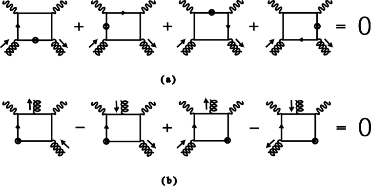
FIG. 8.: A diagrammatic representation of the consistency relations among loop functions resulting from our freedom to choose the routing of the transverse momentum.

The contributions to $(2,0)$ are calculated according to the prescription mentioned before. We send a small amount of transverse momentum into the quark loop through the incoming gluon and remove it through the outgoing. Internal propagators which carry this momentum are then broken successively by the operator $i\gamma_{\perp}$. Since we have a loop, we are given a choice of which way to route the momentum. Either choice must yield the same result, so we immediately have a set of relations among diagrams. As before, our new vertices differ only trivially from gluon insertions. Hence the relations between the $(2,0)$ diagrams translate immediately into consistency requirements on the functions $A_{i}(x,y)$, $B_{i}(x,y)$, and $C_{i}(x,y)$. Six relations follow from the two diagramatic requirements shown in Fig. 8. They are

$$A_{1}(0,x)+B_{1}(x,x)+C_{2}(x,0)+C_{1}(x,0) = 0\;\;,$$ (105)

$$B_{1}(0,x)+A_{1}(x,x)+A_{2}(x,0)+A_{1}(x,0) = 0\;\;,$$ (106)

$$C_{1}(0,x)+C_{1}(x,x)+B_{2}(x,0)+B_{1}(x,0) = 0\;\;,$$ (107)

$$A_{2}(x,x)-C_{2}(-x,-x)+B_{2}(0,x)-C_{2}(0,-x) = 0\;\;,$$ (108)

$$B_{2}(x,x)-B_{2}(-x,-x)+A_{2}(0,x)-A_{2}(0,-x) = 0\;\;,$$ (109)

$$C_{2}(x,x)-A_{2}(-x,-x)+C_{2}(0,x)-B_{2}(0,-x) = 0\;\;.$$ (110)

These relations provide a welcome check of our calculation, as all of the expressions involved are extremely complicated. A similar set of relations can be derived in the non-singlet sector by allowing the transverse momentum to flow through an internal gluon propagator. However, in this case the relations we would derive are not as useful.

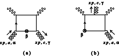
FIG. 9.: The two independent contributions to $M^{\mu+\alpha\beta\gamma\;(g)}_{(2,0)}$

Using exactly the same technique that allowed us to derive the consistency relations, we can obtain an expression for the full contribution to $(2,0)$. There are eight distinct diagrams, of which only two are independent. The diagrams in Fig. 9 $(a)$ and $(b)$ have the value

$$M^{\mu+\alpha\beta\gamma\;(g)}_{(2,0)a}=\left(T_{F}\delta^{ac}\right)\,{\langle e_{q}^{2}\rangle\over\nu}\left[-A_{1}(\tilde{x},\tilde{x})g_{\perp}^{\mu\alpha}g_{\perp}^{\beta\gamma}-B_{1}(\tilde{x},\tilde{x})g_{\perp}^{\mu\beta}g_{\perp}^{\gamma\alpha}-C_{1}(\tilde{x},\tilde{x})g_{\perp}^{\mu\gamma}g_{\perp}^{\alpha\beta}\right]\;\;,$$ (111)

$$M^{\mu+\alpha\beta\gamma\;(g)}_{(2,0)b}=\left(T_{F}\delta^{ac}\right)\,{\langle e_{q}^{2}\rangle\over\nu}\left[\phantom{-}A_{2}(0,\tilde{x})g_{\perp}^{\mu\beta}g_{\perp}^{\gamma\alpha}+B_{2}(0,\tilde{x})g_{\perp}^{\mu\alpha}g_{\perp}^{\beta\gamma}+C_{2}(0,\tilde{x})g_{\perp}^{\mu\gamma}g_{\perp}^{\alpha\beta}\right]\;\;,$$ (112)

respectively. Adding the remaining diagrams and including a symmetry factor of 1/2, we find the full contribution to $(2,0)$ :

$$T^{\mu+\;(g)}_{(2,0)}=T_{F}\,{\langle e_{q}^{2}\rangle\over\nu}\,\int dx \,\left[-p_{1}(-\tilde{x})g^{\mu\alpha}_{\perp}g_{\perp}^{\beta\gamma}+p_{2}(\tilde{x})g_{\perp}^{\mu\beta}g_{\perp}^{\gamma\alpha}+p_{1}(\tilde{x})g_{\perp}^{\mu\gamma}g_{\perp}^{\alpha\beta}\right]\,(\Gamma_{2gB})_{\gamma\beta\alpha}(x)\;\;;$$ (113)

$$p_{1}(x) = A_{1}(-x,-x)-C_{1}(x,x)+C_{2}(0,x)-B_{2}(0,-x)\;\;,$$ (114)

$$p_{2}(x) = B_{1}(-x,-x)-B_{1}(x,x)-A_{2}(0,x)+A_{2}(0,-x)\;\;,$$ (115)

$$(\Gamma_{2gB})_{\alpha\beta\gamma}(x) = \int\,{d\lambda\over 2\pi}\,e^{i\lambda x}\left\langle PS\left|A^{a}_{\alpha}(0)i\partial_{\beta}A^{a}_{\gamma}(\lambda n)\right|PS\right\rangle\;\;.$$ (116)

Since our amplitude is required to be symmetric under $(x_{B}\rightarrow-x_{B})$, the fact that $p_{2}(x)$ is an odd function of $x$ implies immediately that it is zero. This allows us to write the full $(2,0)$ contribution as

$$T^{\mu+\;(g)}_{(2,0)}=2T_{F}\,{\langle e_{q}^{2}\rangle\over\nu}\,\int dx\,p_{1}(\tilde{x})(\Gamma_{2gB})^{\mu\alpha}_{\;\;\alpha}(x)\;\;.$$ (117)

To properly combine with the $(3,0)$ contribution, it would seem that we must have

$$p_{1}(x)=-{1\over 4}f(x,x)\;\;.$$ (118)

However, using the relations (105-110) one can show that

$$p_{1}(x)=-{1\over 2}f(x,x)\;\;.$$ (119)

At first glance, this is disastrous. It looks very much like we have made a mistake. On the other hand, we have been very careful to include all of the appropriate symmetry factors and counting. Going back through the analysis, one has no choice but to conclude that it is correct. The answer to our problem lies in a more subtle place. Looking at $(\Gamma_{3gB})^{\mu\alpha}_{\;\;\alpha}(x,y)$, we see that it has the peculiar property

$$\int\,dx\,(\Gamma_{3gB})^{\mu\alpha}_{\;\;\alpha}(x,y)=0\;\;.$$ (120)

Hence there is an ambiguity in our result. Any function $g(y)$ which is independent of $x$ can be added to $f(x,y)$ to form an equally acceptable amplitude. The contributing part of $f(x,y)$ is actually the modified function $f(x,y)-f(0,y)$. The nature of this ambiguity is that it does not affect the $(3,0)$ contribution to our amplitude. However, it certainly will affect the $(2,0)$ part when one sets $x=y$. One can easily show that the modified function satisfies

$$p_{1}(x)=-{1\over 4}\left(f(x,x)-f(0,x)\right)\;\;,$$ (121)

as required by gauge invariance. Defining the gauge invariant function

$${1\over 4}\,xy\,\left[\Gamma^{\mu\alpha}_{2gB\;\;\alpha}(x,y)+\Gamma^{\mu\alpha}_{3gB\;\;\alpha}(x,y)\right]$$ (122)

$$\qquad=\int\,{d\lambda\over 4\pi}\,{d\mu\over 4\pi}\,e^{i\lambda x}\,e^{i\mu(y-x)}\left\langle PS\left|F^{+\mu}(0)iD^{\perp}_{\alpha}(\mu n)F_{\perp}^{+\alpha}(\lambda n)\right|PS\right\rangle$$ (123)

$$\qquad\qquad\qquad\qquad=i\epsilon^{-+\alpha\mu}MS_{\alpha}\,K_{gB}(x,y)\;\;,$$ (124)

and substituting the explicit expression for $f(x,y)$, one arrives at the full gluon contribution:

$$S_{T}^{(1)g}(\nu,Q^{2}) = {\alpha_{s}(Q^{2})n_{f}T_{F}\over 2\pi}\,\langle e_{q}^{2}\rangle\int\,{dx\,dy\over xy(y-x)}\,\left[M^{g}\left({x\over x_{B}},{y\over x_{B}}\right)\right.$$ (126)

$$\phantom{{\alpha_{s}(Q^{2})n_{f}T_{F}\over 2\pi}\,\langle e_{q}^{2}\rangle\int\,{dx\,dy\over xy(y-x)}[\qquad}\left.\vphantom{M^{g}\left({x\over x_{B}},{y\over x_{B}}\right)}-(x_{B}\rightarrow-x_{B})\right]K_{gB}(x,y)\;\;;$$

$$M^{g}(x,y) = {1\over xy}\,$$ (136)

$$\!\!\!\!\!\!\!\!\!\times\left\{{2\over\epsilon}\left({Q^{2}e^{\gamma}\over 4\pi\mu^{2}}\right)^{-\epsilon/2}\left[\vphantom{\left((x+y)(2x+3y)\over x-y\right)}\left((y-2x)(1-x)+3y(y-x)-6\,{y\over x}\,(y-x)\right)\log\left(1-x\right)\right.\right.$$

$$+\left((4x-3y)(1-y)+4x(y-x)-8\,{x\over y}\,(y-x)\right)\log\left(1-y\right)$$

$$\left.+\left({(x+y)(2x-3y)\over x-y}(1-(x-y))-xy\right)\log\left(1-(x-y)\right)\right]$$

$$-3\left(y+2\,{(y-x)^{2}\over x}\right)(1-x)\log(1-x)$$

$$+\left(3(4x-3y)(1-y)+14x(y-x)-20\,{x\over y}\,(y-x)\right)\log(1-y)$$

$$+{6x^{2}+xy-9y^{2}\over x-y}(1-(x-y))\log\left(1-(x-y)\right)$$

$$-{1\over 2}\left((y-2x)(1-x)+3y(y-x)-6\,{y\over x}\,(y-x)\right)\log^{2}\left(1-x\right)$$

$$-{1\over 2}\left((4x-3y)(1-y)+4x(y-x)-8\,{x\over y}\,(y-x)\right)\log^{2}\left(1-y\right)$$

$$\left.-{1\over 2}\left({(x+y)(2x-3y)\over x-y}(1-(x-y))-xy\right)\log^{2}\left(1-(x-y)\right)\vphantom{{2\over\epsilon}\left({Q^{2}e^{\gamma}\over 4\pi\mu^{2}}\right)^{-\epsilon/2}}\right\}\;\;,$$

which is identical to that in Ref. [26] and agrees with the results of Ref. [27] after one has transformed into their basis.

As before, the divergent part of this expression generates the evolution of the leading distribution. In this case, it contributes an extra term to the singlet quark distribution,

$$K_{S}(x,y,Q^{2})\equiv\sum_{q}K_{q}(x,y,Q^{2})\;\;,$$ (137)

that is not present in the nonsinglet sector :

$$\int\,dx \left({1\over x-x_{B}}-{1\over x+x_{B}}\right)\,Q^{2}\,{d\over dQ^{2}}q^{S}_{T}(x,Q^{2})={\alpha_{s}(Q^{2})n_{f}T_{F}\over 2\pi}\int\,{dx\,dy\over x^{2}y^{2}(y-x)}$$ (142)

$$\times\left[\vphantom{x_{B}\over y}\left((y-2x)(x_{B}-x)+3y(y-x)-6\,{x_{B}y\over x}\,(y-x)\right)\log\left(1-{x\over x_{B}}\right)\right.$$

$$\quad+\left((4x-3y)(x_{B}-y)+4x(y-x)-8\,{x_{B}x\over y}\,(y-x)\right)\log\left(1-{y\over x_{B}}\right)$$

$$\quad\left.+\left({(x+y)(2x-3y)\over x-y}\,(x_{B}-(x-y))-xy\right)\log\left(1-{x-y\over x_{B}}\right)\right.$$

$$\qquad\qquad\left.\vphantom{{x_{B}\over y}}-(x_{B}\rightarrow-x_{B})\right]K_{g}(x,y,Q^{2})+\cdots\;\;,$$

where the ellipses denote terms given by Eq. (90) above.

At this point, one can easily obtain an expression for $g_{T}(x_{B},Q^{2})$ by taking the imaginary part of Eq. (126) as $x_{B}$ approaches the positive $x$-axis from below. This is done explicitly in Ref. [10].

V The Operator Product Expansion

So far, our results have been expressed in terms of nonlocal parton correlation functions. While these distributions are easy to interpret, they do not allow one to exploit the full symmetry of our theory. In particular, they do not lend themselves to a straightforward twist analysis. Furthermore, their evolution equations are unnecessarily complicated.

To obtain an expression with explicit twist separation, we cast our result in the form of an operator product expansion of two electromagnetic currents. The idea behind this approach is that for large $Q^{2}$, the electromagnetic currents in the definition of $T^{\mu\nu}$ are separated approximately along the light-cone direction $n^{\mu}$. Such operator products can be expressed as an infinite sum of local operators in the same way that a Taylor series can be used to represent a function. Since local operators can be separated into irreducible representations of the Lorentz group, they are easier to classify and their evolution is somewhat more constrained.

One can obtain the operator product expansion by expanding our previous results about $x_{B}=\infty$ :

$$S_{T}(\nu,Q^{2})=\sum_{n=0}^{\infty}s_{n}(Q^{2})\left({1\over x_{B}}\right)^{2n+1}\;\;.$$ (143)

Although this expansion takes place in the unphysical region $x_{B}>1$, its terms are related to moments of the physical structure function, $g_{T}(x_{B},Q^{2})$ through dispersion relations :

$$\int_{0}^{1}\,dx\,x^{2n}g_{T}(x,Q^{2})={1\over 4}\,s_{n}(Q^{2})\;\;.$$ (144)

This shows why the operator product expansion is experimentally relevant.

At leading order in $\alpha_{s}$, it is quite trivial to expand our result. We obtain

$$s_{n}^{(0)}(Q^{2})=2\sum_{q}e_{q}^{2}\int^{1}_{-1}\,dx\,x^{2n}\,q_{T}(x,Q^{2})\;\;.$$ (145)

From the definition of $q_{T}(x,Q^{2})$, one can show that

$$\int^{1}_{-1}\,dx\,x^{2n}\,q_{T}(x,Q^{2})=-{1\over 2M^{2}}\left\langle PS\left|\overline{\psi}_{q}iD_{\mu_{1}}iD_{\mu_{2}}\cdots iD_{\mu_{2n}}\gamma_{\alpha}\gamma_{5}\psi_{q}\right|PS\right\rangle n^{\mu_{1}}\cdots n^{\mu_{2n}}MS^{\alpha}\;\;.$$ (146)

Substituting this result into Eq. (144) gives us an expression for the $(2n+1)$-th moment of the physical structure function in terms of the matrix element of a local operator.

The different components of the operator above do not constitute an irreducible representation of the Lorentz group. As such, they are not constrained to have simple properties as the renormalization scale is changed or higher-order radiative corrections are taken into account. A more useful basis is one which forms irreducible representations of the Lorentz group. Such a basis will be useful at arbitrary orders in perturbation theory, as the behavior of its elements under renormalization is restricted by the space-time symmetry. A standard analysis of the Lorentz group tells us that the components of the operators

$${}_{q}\theta_{n+1,2}^{\mu_{1}\cdots\mu_{n+1}} = \overline{\psi}_{q}iD^{(\mu_{1}}\cdots iD^{\mu_{n}}\gamma^{\mu_{n+1})}\gamma_{5}\psi_{q}\;\;,$$ (147)

$${}_{q}\theta_{n,3}^{\lambda\mu_{1}\cdots\mu_{n}} = \overline{\psi}_{q}iD^{(\mu_{1}}\cdots iD^{[\mu_{n})}\gamma^{\lambda]}\gamma_{5}\psi_{q}\;\;,$$ (148)

where $(\cdots)$ denotes symmetrization of indices and the removal of all traces and $[\cdots]$ indicates antisymmetrization of indices, form irreducible representations. Taking

$$\left\langle PS\left|\,{}_{q}\theta_{n+1,2}^{\mu_{1}\cdots\mu_{n+1}}\right|PS\right\rangle = 2a_{n}^{q}(Q^{2})\,MS^{(\mu_{1}}P^{\mu_{2}}\cdots P^{\mu_{n+1})}\;\;,$$ (149)

$$\left\langle PS\left|\,{}_{q}\theta^{\lambda\mu_{1}\cdots\mu_{n}}_{n,3}\right|PS\right\rangle = 2d_{n}^{q}(Q^{2})\,MS^{[\lambda}P^{(\mu_{1}]}\cdots P^{\mu_{n})}\;\;,$$ (150)

we see that the matrix elements of every component of $\theta_{n,3}$ are kinematically suppressed by at least one power of $Q$ in relation to the $+\cdots+$ component of $\theta_{n+1,2}$. This suppression is characterized by the twist of the operator, defined as mass dimension minus spin. Since $\theta_{n+1,2}$ has spin $n+1$ and $\theta_{n,3}$ has spin $n$, the fully symmetric operators have twist-two and the operators of mixed symmetry have twist-three for all values of $n$. It is generally true that operators of twist $t$ are kinematically suppressed by at least $(\Lambda_{\rm QCD}/Q)^{t-2}$. However, as exemplified by relations in Eqs. (149, 150), all of the relevant information can be extracted at ${\cal O}(\Lambda_{\rm QCD}/Q)^{t-2}$.

In our case, $S_{T}$ contains contributions from twist-two and -three. However, since the twist-two information can be extracted from the leading scaling function $g_{1}(x_{B},Q^{2})$, only the twist-three contributions are new. To see this explicitly, we transform Eq. (146) to the new basis and write [18]

$$s_{n}^{(0)}(Q^{2})={2\over 2n+1}\sum_{q}e_{q}^{2}\left[a^{q}_{2n}(Q^{2})+2n\,d^{\,q}_{2n}(Q^{2})\right]\;\;.$$ (151)

An analysis of the leading contributions to $T^{\mu\nu}$ [15] leads one to the moment relations

$$\int_{0}^{1}\,dx\,x^{n}\,g^{(0)}_{1}(x,Q^{2})={1\over 2}\sum_{q}e_{q}^{2}\,a_{n}^{q}(Q^{2})\;\;,$$ (152)

which allows us to isolate the pure twist-three information [23]:

$$\int_{0}^{1}\,dx\,x^{n}\,\left[g^{(0)}_{T}(x,Q^{2})-{1\over n+1}\,g^{(0)}_{1}(x,Q^{2})\right]={n\over 2(n+1)}\,\sum_{q}e_{q}^{2}\,d_{n}^{q}(Q^{2})\;\;.$$ (153)

One of the main purposes of this paper is to present the one-loop corrections to Eq. (153). In particular, it will be interesting to see whether or not the twist-three information is isolated by the same combination of $g_{T}$ and $g_{1}$ at higher orders. A priori, there doesn’t seem to be any reason why it should be. This statement is really nothing more than a relation between $g_{1}$ and the twist-two part of $g_{T}$. It seems to depend on the operator (146) relevant to $g_{T}$. In fact, we will see that this particular combination of $g_{T}$ and $g_{1}$ does isolate pure twist-three effects at one-loop order. This fact asserts a kinematic rather than dynamic relationship between these two quantities, as will become clear below.

In order to separate the twist-two and -three parts of our one-loop amplitudes, we must find an unambiguous way to tell the difference between these contributions. Since one cannot form a mixed-symmetry operator with only partial derivatives, $\partial_{\perp}$ cannot appear in the twist-three part of the expansion. This allows us to use the partial derivative terms in our distributions to identify the coefficients of the twist-two operators. Completing the operators using the definition in Eq. (147), we identify the remainder of the expansion as purely twist-three.

Before we can systematically express the twist-three contribution as a sum of local operators, we must identify an operator basis in which to express it. Unfortunately, the operator $\theta_{n,3}$ is not sufficient for our needs. One can immediately see this by looking at our expression (86) for the one-loop contribution. Our expansion will involve general moments of the functions $K_{q}(x,y,Q^{2})$ rather than the simple functions $q_{T}(x,Q^{2})$. These moments are directly related to matrix elements of operators of the form

$$\overline{\psi}_{q}\left(i\partial^{+}\right)^{i}iD_{\perp}^{\lambda}\left(i\partial^{+}\right)^{n-i}\not\!n\gamma_{5}\psi_{q}\;\;,$$ (154)

but these operators have no definite twist and are not useful for our purposes. A useful basis of twist-three operators in the nonsinglet sector was first identified in [20]. The operators

$${}_{q}R_{n,j}^{\sigma\mu_{1}\cdots\mu_{n}} = \overline{\psi}_{q}iD^{(\mu_{1}}\cdots iD^{\mu_{j-1}}\left(-igF^{\sigma\mu_{j}}\right)iD^{\mu_{j+1}}\cdots iD^{\mu_{n-1}}\gamma^{\mu_{n})}\gamma_{5}\psi\;\;,$$ (155)

$${}_{q}S_{n,j}^{\sigma\mu_{1}\cdots\mu_{n}} = \overline{\psi}_{q}iD^{(\mu_{1}}\cdots iD^{\mu_{j-1}}\left(g\tilde{F}^{\sigma\mu_{j}}\right)iD^{\mu_{j+1}}\cdots iD^{\mu_{n-1}}\gamma^{\mu_{n})}\psi\;\;;$$ (156)

$${}_{q}W^{\sigma\mu_{1}\cdots\mu_{n}}_{n,j} = {}_{q}S_{n,j}^{\sigma\mu_{1}\cdots\mu_{n}}+_{q}S_{n,n-j}^{\sigma\mu_{1}\cdots\mu_{n}}+_{q}R_{n,j}^{\sigma\mu_{1}\cdots\mu_{n}}-_{q}R_{n,n-j}^{\sigma\mu_{1}\cdots\mu_{n}}\;\;,$$ (157)

for $j=1$ to $n-1$, satisfy

$$\int\,{dx\,dy\over xy}\,y^{j}\,x^{n-j}\,(y-x)\,K_{q}(x,y,Q^{2})=-{1\over 8}\,w_{n,j}^{q}(Q^{2})\;\;,$$ (158)

where

$$\left\langle PS\left|\,{}_{q}W_{n,j}^{\sigma\mu_{1}\cdots\mu_{n}}\right|PS\right\rangle=2w_{n,j}^{q}(Q^{2})MS^{[\sigma}P^{(\mu_{1}]}\cdots P^{\mu_{n})}\;\;.$$ (159)

Note the appearance of the field strength tensor in our operator basis. Since there can be no partial derivative contributions to the twist-three part of our expansion, this is required by gauge invariance.

Expanding $S_{T}^{NS(1)}$ in Eq. (75) about $x_{B}=\infty$ and using Eq. (158), we find

$$S_{T}^{NS(1)}(\nu,Q^{2})={\alpha_{s}(Q^{2})\over 4\pi}\,\sum_{q}\hat{e}_{q}^{2}\sum_{n\;{\rm even}=2}^{\infty}\,\left({1\over x_{B}}\right)^{n+1}\left[\vphantom{-\sum_{j=1}^{n-1}\,c_{n,j}^{3NS}\,w_{n,j}^{q}(Q^{2})}{2\over n+1}\,c_{n}^{2NS}\,a_{n}^{q}(Q^{2})\right.$$ (160)

$$\phantom{S_{T}^{NS(1)}(\nu,Q^{2})={\alpha_{s}(Q^{2})\over 4\pi}\,\sum_{q}\hat{e}_{q}^{2}\sum_{n\;even=2}^{\infty}\,\left({1\over x_{B}}\right)^{n+1}[}\left.\qquad-\sum_{j=1}^{n-1}\,c_{n,j}^{3NS}\,w_{n,j}^{q}(Q^{2})\right]\;\;;$$ (161)

$$c_{n}^{2NS}=C_{F}\left\{4T^{1}_{1}(n)-4S_{2}(n)+\left[3+{2\over n+1}+{2\over n+2}\right]S_{1}(n)+{8\over n+2}-{2\over n+1}-9\right\}\;\;,$$ (162)

$$c_{n,j}^{3NS}=(n-j)\left[{C_{F}\over 2}\left({1\over n+1}-{2\over n+2}\right)-{1\over 2(n+1)}c_{n}^{2NS}-{C_{A}\over 2}\,{1\over n+2}\,\left(2+S_{1}(n+1)\right)\right]$$ (163)

$$\phantom{c_{n,j}^{3NS}=}+{C_{A}\over 2}\left[S_{1}(n)-S_{1}(j)\right]+\left(C_{F}-{C_{A}\over 2}\right)\left\{\vphantom{\left[{1\over n+1}{n-1\choose j-1}-\sum_{k=j}^{n-1}{k-1\choose j-1}{2+S_{1}(k)\over k+1}\right]}{1\over n+2}\left(2+S_{1}(n+1)\right)-{1\over n+1}\right.$$ (164)

$$\left.\phantom{c_{n,j}^{3NS}=\left(C_{F}-{C_{A}\over 2}\right)\{}+(-1)^{j}\left[\vphantom{+{1\over n+1}{n-1\choose j-1}-\sum_{k=j}^{n-1}{k-1\choose j-1}{2+S_{1}(k)\over k+1}}{1\over n+2}\left[{n-1\choose j}-{n-1\choose j-1}\right]\left(2+S_{1}(n+1)\right)\right.\right.$$ (165)

$$\left.\left.\phantom{c_{n,j}^{3NS}=\left(C_{F}-{C_{A}\over 2}\right)\{}\qquad+{1\over n+1}{n-1\choose j-1}-\sum_{k=j}^{n-1}{k-1\choose j-1}{2+S_{1}(k)\over k+1}\right]\right\}\;\;,$$ (166)

where we have defined

$$S_{j}(n)=\sum_{i=1}^{n}{1\over i^{j}}\;\;,$$ (167)

$$T^{k}_{j}(n)=\sum_{i=1}^{n}{S_{j}(n)\over i^{k}}\;\;.$$ (168)

In the above form, it is easy to see how much the result deviates from the naive expectation that only the twist-three part of $q_{T}(x,Q^{2})$ will contribute to $S_{T}$. The ‘simple’ twist-three operator $\theta_{n,3}$ takes the form

$$\theta_{n,3}^{\lambda\mu_{1}\cdots\mu_{n}}={1\over 4n}\sum_{j=1}^{n-1}(n-j)W^{\lambda\mu_{1}\cdots\mu_{n}}_{n,j}$$ (169)

in the complete basis [20]. In deriving this result, the equation of motion has been repeatedly used. Also, like many of the operator relations in this paper, this equation is valid only for forward matrix elements. Looking at Eq. (164), we see that only the first term respects the naive expectation. Taking the large-$N_{c}$ limit, which simplifies the evolution of $q_{T}(x,Q^{2})$ as we will see below, gets rid of most of the complicated $j$-dependence of our result, but fails to remove the second term. All of the $w_{n,j}^{q}$ enter nontrivially in the NLO result for $S_{T}^{NS}$. This fact will complicate precision analysis of $g_{T}(x,Q^{2})$ data immensely.

Since the operators $W_{n,j}$ for different values of $j$ all have the same mass-dimension and transform in the same way under Lorentz rotations, they may mix with each other under renormalization. This is the origin of all of our difficulties with the evolution of $q_{T}(x,Q^{2})$. Since we have no more symmetries to constrain the form of our result, a different combination of the $W_{n,j}$ will appear at each new order in $\alpha_{s}$.

Expanding Eq. (90) about $x_{B}=\infty$, imposing order-by-order equality, and transforming to the standard basis, one arrives at evolution equations for the scalar matrix elements of our local operators :

$$Q^{2}{d\over dQ^{2}} a_{n}^{NS}(Q^{2})={\alpha_{s}(Q^{2})\over 2\pi}C_{F}\left[{3\over 2}+{1\over(n+1)(n+2)}-2S_{1}(n+1)\right]a_{n}^{NS}(Q^{2})\;\;,$$ (170)

$$Q^{2}{d\over dQ^{2}} \sum_{j=1}^{n-1}(n-j)w_{n,j}^{NS}(Q^{2})={\alpha_{s}(Q^{2})\over 2\pi}\,\sum_{j=1}^{n-1}\left\{\vphantom{+(-1)^{j}\left({1\over n+2}\left({n-1\choose j}-{n-1\choose j-1}\right)-\sum_{k=j}^{n-1}{1\over k+1}{k-1\choose j-1}\right)}C_{F}\left[{3\over 2}+{1\over(n+1)(n+2)}-2S_{1}(n+1)\right]\right.$$ (173)

$$-{C_{A}\over 2}\,{n+1\over n+2}+\left(C_{F}-{C_{A}\over 2}\right){n+1\over n-j}\left[\vphantom{+(-1)^{j}\left({1\over n+2}\left({n-1\choose j}-{n-1\choose j-1}\right)-\sum_{k=j}^{n-1}{1\over k+1}{k-1\choose j-1}\right)}{1\over n+2}\right.$$

$$\left.\left.\!\!\!\!\!\!\!\!\!\!\!+(-1)^{j}\left({1\over n+2}\left({n-1\choose j}-{n-1\choose j-1}\right)-\sum_{k=j}^{n-1}{1\over k+1}{k-1\choose j-1}\right)\right]\right\}(n-j)w_{n,j}^{NS}(Q^{2})\;\;.$$

From these equations, it is quite clear that diagonal evolution of ${}_{NS}\theta_{n,3}$ is broken only by terms of order $1/N_{c}^{2}$ in the large-$N_{c}$ limit. This fact was first recognized by Ali, Braun and Hiller [21] in 1991. Its anomalous dimension in this limit is reproduced by this equation. The evolution of the $w_{n,j}^{NS}(Q^{2})$ was first obtained by Bukhostov, Kuraev, and Lipatov (BKL) [20], and our result agrees with theirs. Therefore, we conclude that the amplitude is factorizable at this order. In addition, we reproduce the well-known anomalous dimensions of the twist-two operators ${}_{NS}\theta_{n+1,2}$ [2].

In the singlet sector, things become somewhat more complicated. Here, we must introduce an extra factor of $1/xy$ to obtain gauge-invariance. To generate a local gauge-invariant operator product expansion, it would seem that this factor must be canceled by the kernel $M^{g}(x,y)$. As argued above, one must define $M^{g}(x,y)$ in such a way that $M^{g}(0,y)=0$. Hence, the only nontrivial requirement seems to be $M^{g}(x,0)=0$. Checking this explicitly, we see that it is not the case. From this result, one might conclude that a local gauge-invariant operator product expansion does not exist for $S_{T}$ in the singlet channel. However, a more careful analysis brings a quite different result.

The first step in a systematic approach to this problem lies in identifying and separating out the twist-two part of our amplitude. Since we know that partial derivative terms belong exclusively to this part of the amplitude, we can use them as a guide once more. In analogy with the nonsinglet sector, we write the twist-two operators

$${}_{g}\theta^{\mu_{1}\cdots\mu_{n+1}}_{n+1,2}=F^{\alpha(\mu_{1}}iD^{\mu_{2}}\cdots iD^{\mu_{n}}i\tilde{F}^{\mu_{n+1})}_{\;\;\alpha}\;\;,$$ (174)

where the dual field strength tensor is defined by $\tilde{F}^{\mu\nu}\equiv{1\over 2}\epsilon^{\mu\nu\alpha\beta}F_{\alpha\beta}$. Taking the $(i+\cdots+)$ component and simplifying, we obtain

$${}_{g}\theta_{n+1,2}^{i+\cdots+} = {2\over n+1}\epsilon^{ij}\left[\vphantom{\sum_{m=0}^{n-1}}(n+1)iA^{j}(i\partial^{+})^{n}i\partial^{k}A^{k}+iA^{j}(i\partial^{+})^{n-1}D_{\alpha}F^{\alpha+}\right.$$ (176)

$$+\left.f^{abc}A_{a}^{j}(i\partial^{+})^{n-1}gA_{b}^{k}i\partial^{+}A_{c}^{k}+\sum_{m=0}^{n-1}f^{abc}A_{a}^{j}(i\partial^{+})^{m}gA_{b}^{k}(i\partial^{+})^{n-m}A_{c}^{k}\right]\;\;.$$

Here, the indices $(i,j,k)$ represent transverse dimensions. Note that a sign has been taken into account for transverse partial derivatives and gauge fields with contravariant indices. There are several important features of this operator. One is the appearence of the operator $D_{\alpha}F^{\alpha+}$. Through the gluon equations of motion, this term transmutes into a quark singlet contribution. It will generate a difference between the behavior of the singlet and nonsinglet twist-three quark operators under renormalization and their contributions to the operator product expansion. At present, its most striking feature is that it contains terms which can be generated by $M^{g}(x,0)$. This suggests that separating the twist-two contribution, whose gauge invariance and locality are not in question, from the amplitude before worrying about the issues of gauge invariance may lead us to the correct understanding of our result.

In order to perform a straightforward separation, it is advantageous for us to write the three-gluon part of our amplitude in such a way that the bosonic symmetry is evident. As we have seen above, forgetting this symmetry can easily lead to incorrect conclusions. To this end, we define the local operator

$${\cal O}_{n,j}^{\mu}=igf^{abc}A_{a}^{\mu}\left[(i\partial^{+})^{j}A_{\alpha}^{b}\right]\left[(i\partial^{+})^{n-j}A_{c}^{\alpha}\right]$$ (177)

and re-write our twist-two operator in terms of it :

$${}_{g}\theta_{n+1,2}^{i+\cdots+}=-{2\over n+1}\epsilon^{ij} \left\{\vphantom{-i\sum_{j=1}^{n-1}\left[{n-1\choose j}+{n\choose j+1}\right]{\cal O}_{n,j}}(n+1)iA^{j}iD^{\perp}_{\sigma}(i\partial^{+})^{n}A_{\perp}^{\sigma}-iA^{j}(i\partial^{+})^{n-1}D_{\alpha}F^{\alpha+}\right.$$ (179)

$$\left.-i\sum_{k=1}^{n-1}\left[{n-1\choose k}+{n\choose k+1}\right]{\cal O}_{n,k}^{j}\right\}\;\;.$$

This equation is valid modulo total derivatives. Note that bosonic symmetry implies ${\cal O}^{\mu}_{n,j}=-{\cal O}^{\mu}_{n,n-j}$. Our full amplitude takes the form

$$T^{\mu+(1)}_{g} = {\alpha_{s}n_{f}T_{F}\over 2\pi}\,{\langle e_{q}^{2}\rangle\over\nu}\sum_{n\;\;{\rm even}=2}^{\infty}\left({1\over x_{B}}\right)^{n}$$ (182)

$$\times\left\{\vphantom{-{2\over(n+1)(n+2)}\left[S_{1}(n)+2\right]\sum_{j=1}^{n-1}{n\choose j+1}\left\langle PS\left|{\cal O}^{\mu}_{n,j}\right|PS\right\rangle}4\left[{2\over n+2}-{1\over n+1}\right]\left[S_{1}(n)+1\right]\left\langle PS\left|A^{\mu}iD^{\perp}_{\sigma}(i\partial^{+})^{n}A_{\perp}^{\sigma}\right|PS\right\rangle\right.$$

$$\left.\phantom{\times\{}-{2\over(n+1)(n+2)}\left[S_{1}(n)+2\right]\sum_{j=1}^{n-1}{n\choose j+1}\left\langle PS\left|{\cal O}^{\mu}_{n,j}\right|PS\right\rangle\right\}\;\;,$$

where the divergent part has been ignored. It can be restored via the substitution

$$S_{1}(n)\rightarrow{2\over\epsilon}\left({Q^{2}e^{\gamma}\over 4\pi\mu^{2}}\right)^{-\epsilon/2}+S_{1}(n)\;\;.$$ (183)

In this form, it is easy to separate the twist-two and -three parts of the amplitude. We have only to identify an appropriate basis of twist-three gluonic operators to write the final result. An appropriate basis takes

$${}_{g}S_{n,j}^{\lambda\mu_{1}\cdots\mu_{n}} = F^{\alpha(\mu_{1}}iD^{\mu_{2}}\cdots iD^{\mu_{j-1}}ig\tilde{F}^{\lambda\mu_{j}}iD^{\mu_{j+1}}\cdots iD^{\mu_{n-1}}F^{\mu_{n})}_{\;\;\alpha}\;\;,$$ (184)

$${}_{g}W_{n,j}^{\lambda\mu_{1}\cdots\mu_{n}} = {}_{g}S_{n,j}^{\lambda\mu_{1}\cdots\mu_{n}}+\,_{g}S_{n,n-j+1}^{\lambda\mu_{1}\cdots\mu_{n}}$$ (185)

for $j=2$ to $n-1$. The analogue of ${}_{q}R_{n,j}$ is not independent in this case since

$$F^{\alpha+}(i\partial^{+})^{i}\tilde{F}^{\lambda+}(i\partial^{+})^{j}F^{+}_{\;\;\alpha}=F^{\alpha+}(i\partial^{+})^{i}F^{+}_{\;\;\alpha}(i\partial^{+})^{j}\tilde{F}^{\lambda+}+F^{\lambda+}(i\partial^{+})^{i}\tilde{F}^{\alpha+}(i\partial^{+})^{j}F^{+}_{\;\;\alpha}\;\;.$$ (186)

Note that our basis differs from that found in Ref. [20]. Through repeated partial integration and binomial coefficient sums, one can show that the relation

$$\sum_{j=1}^{n-1}c_{n,j}{\cal O}^{\mu}_{n,j}=i\epsilon^{\mu+-\beta}g_{\beta\lambda}\sum_{j=2}^{n-1}{1\over 2}\sum_{k=j}^{n-1}(-1)^{k+1}c_{n,k}\,{}_{g}W^{\lambda+\cdots+}_{n,j}$$ (187)

is valid for forward matrix elements. It is this expression that establishes the gauge invariance of our result. Defining scalar matrix elements in exact analogy to the nonsinglet sector, we find the following result for the singlet part of $S_{T}^{(1)}$ :

$$S_{T}^{S(1)}(\nu,Q^{2})={\alpha_{s}(Q^{2})n_{f}T_{F}\over 2\pi}\,\langle e_{q}^{2}\rangle\sum_{n\;{\rm even}=2}^{\infty}\,\left({1\over x_{B}}\right)^{n+1}$$ (188)

$$\qquad\times\left\{{2n\over(n+1)^{2}(n+2)}\left(S_{1}(n)+1\right)\left[-2a_{n}^{g}(Q^{2})+\sum_{j=1}^{n-1}{n-2\choose j-1}(-1)^{j+1}w_{n,j}^{S}(Q^{2})\right]\right.$$ (189)

$$\qquad\qquad\qquad\left.+{1\over 2}\,{1\over(n+1)(n+2)}\sum_{j=2}^{n-1}c_{n,j}^{g}w^{g}_{n,j}(Q^{2})\right\}$$ (190)

$$\qquad\qquad+{\alpha_{s}(Q^{2})\over 4\pi}\,\langle e_{q}^{2}\rangle\sum_{n\;{\rm even}=2}^{\infty}\,\left({1\over x_{B}}\right)^{n+1}\left[{2\over n+1}\,c_{n}^{2NS}\,a_{n}^{S}(Q^{2})-\sum_{j=1}^{n-1}\,c_{n,j}^{3NS}\,w_{n,j}^{S}(Q^{2})\right]\;\;;$$ (191)

$$c_{n,j}^{g}=n-1-{n^{2}+1\over n+1}\left(S_{1}(n)+1\right)$$ (192)

$$\qquad\qquad+2(-1)^{j}{n-1\choose j}\left[1-{(n-1)^{2}+2nj\over n^{2}-1}\left(S_{1}(n)+1\right)\right]\;\;.$$ (193)

Here, the scalar matrix elements of singlet quark operators are defined via

$$a_{n}^{S}(Q^{2}) = \sum_{q}a_{n}^{q}(Q^{2})\;\;,$$ (194)

$$w_{n,j}^{S}(Q^{2}) = \sum_{q}w_{n,j}^{q}(Q^{2})\;\;.$$ (195)

This result was presented in a different operator basis in [27] for $n=2,4,6$.

The evolution in the singlet sector can also be deduced by our results. One obtains

$$Q^{2}{d\over dQ^{2}} a_{n}^{S}(Q^{2})={\alpha_{s}(Q^{2})\over 2\pi}C_{F}\left[{3\over 2}+{1\over(n+1)(n+2)}-2S_{1}(n+1)\right]a_{n}^{S}(Q^{2})$$ (197)

$$\phantom{a_{n}^{S}(Q^{2})}+{\alpha_{s}(Q^{2})\over 2\pi}\,2n_{f}T_{F}\left({2\over n+2}-{1\over n+1}\right)a_{n}^{g}(Q^{2})\;\;,$$

$$Q^{2}{d\over dQ^{2}} \sum_{j=1}^{n-1}(n-j)w_{n,j}^{S}(Q^{2})={\alpha_{s}(Q^{2})\over 2\pi}\,\sum_{j=1}^{n-1}\left\{\vphantom{\left[\left({n\choose j}\right)\right]}C_{F}\left[{3\over 2}+{1\over(n+1)(n+2)}-2S_{1}(n+1)\right]\right.$$ (202)

$$\qquad+4n_{f}T_{F}{(-1)^{j}\over n-j}\,{n\over(n+1)(n+2)}\,{n-2\choose j-1}-{C_{A}\over 2}\,{n+1\over n+2}$$

$$\qquad+\left(C_{F}-{C_{A}\over 2}\right){n+1\over n-j}\left[\vphantom{\left({1\over n+2}\left({n-1\choose j}-{n-1\choose j-1}\right)-\sum_{k=j}^{n-1}{1\over k+1}{k-1\choose j-1}\right)}{1\over n+2}\right.$$

$$\left.\left.+(-1)^{j}\left({1\over n+2}\left({n-1\choose j}-{n-1\choose j-1}\right)-\sum_{k=j}^{n-1}{1\over k+1}{k-1\choose j-1}\right)\right]\right\}(n-j)w_{n,j}^{S}(Q^{2})$$

$$+{\alpha_{s}(Q^{2})\over 4\pi}\,2n_{f}T_{F}\sum_{j=2}^{n-1}{1\over n+2}\left[{n^{2}+1\over n+1}+2(-1)^{j}{n-1\choose j}\,{(n-1)^{2}+2jn\over n^{2}-1}\right]w^{g}_{n,j}(Q^{2})\;\;.$$

Here, also, one reproduces the well-known twist-two result [2]. Use of the equation of motion in the gluonic twist-two operator has generated a term which destroys the autonomous evolution of ${}_{S}\theta_{n,3}$ in the large-$N_{c}$ limit. This behavior can be predicted simply by looking at the diagrams which contribute to evolution in this sector, c.f. [22]. These results were first obtained by BKL [20]. Translating from their basis to ours, we find that there is some disagreement between our results and theirs.

We are now in a position to present the full NLO corrections to Eq. (153). Using the well-known result [32, 33, 34]

$$\int_{0}^{1}x^{n}g_{1}(x,Q^{2}) = {1\over 2}\left[1+{\alpha_{s}(Q^{2})\over 4\pi}\,c^{2NS}_{n}\right]\sum_{q}e_{q}^{2}a_{n}^{q}(Q^{2})$$ (204)

$$-{\alpha_{s}(Q^{2})n_{f}T_{F}\over 2\pi}\,\langle e_{q}^{2}\rangle\,{n\over(n+1)(n+2)}\,\left(S_{1}(n)+1\right)a_{n}^{g}(Q^{2})\;\;,$$

one finds

$$\int_{0}^{1}\,dx\,x^{n} \left(g_{T}(x,Q^{2})-{1\over n+1}\,g_{1}(x,Q^{2})\right)={1\over 8(n+1)}\,\sum_{q}e_{q}^{2}$$ (208)

$$\times\left\{\sum_{j=1}^{n-1}\left[1-{\alpha_{s}(Q^{2})\over 2\pi}\,{n+1\over n-j}\,c_{n,j}^{3NS}\right](n-j)w^{q}_{n,j}(Q^{2})\right.$$

$$\phantom{\times\{}+{\alpha_{s}(Q^{2})T_{F}\over\pi}\,{2n\over(n+1)(n+2)}\left(S_{1}(n)+1\right)\sum_{j=1}^{n-1}\,(-1)^{j-1}{n-2\choose j-1}w_{n,j}^{S}(Q^{2})$$

$$\left.\phantom{\times\{}+{\alpha_{s}(Q^{2})T_{F}\over 2\pi}\,{1\over n+2}\sum_{j=2}^{n-1}c_{n,j}^{g}w^{g}_{n,j}(Q^{2})\right\}+{\cal O}\left(\Lambda_{\rm QCD}/Q,\alpha_{s}^{2}(Q^{2})\right)\;\;.$$

As promised, the relation between $g_{1}$ and the twist-two part of $g_{T}$ is unaffected at this order.

We can gain insight into this phenomenon by stripping away the external states implicit in Eqns.(161,190) and writing the operator product expansion in its full glory :

$$i\int\,d^{4}z \;e^{iq\cdot z}TJ^{[\mu}(z)J^{\nu]}(0)=-i\epsilon^{\mu\nu\alpha\beta}q_{\alpha}g_{\beta\lambda}\,{2\over Q^{2}}\sum_{n\;{\rm even}=2}^{\infty}{(2q_{\mu_{1}})\cdots(2q_{\mu_{n}})\over(Q^{2})^{n}}$$ (214)

$$\times\left\{\vphantom{+{\alpha_{s}(Q^{2})n_{f}T_{F}\over 4\pi}\,\langle e_{q}^{2}\rangle\,{1\over(n+1)(n+2)}\sum_{j=2}^{n-1}c^{g}_{n,j}\,{}_{g}W^{\lambda\mu_{1}\cdots\mu_{n}}_{n,j}}\sum_{q}e_{q}^{2}\left[1+{\alpha_{s}(Q^{2})\over 4\pi}c_{n}^{2NS}\right]\;_{q}\theta_{n+1,2}^{\lambda\mu_{1}\cdots\mu_{n}}\right.$$

$$\phantom{\times\{}-{\alpha_{s}(Q^{2})n_{f}T_{F}\over\pi}\,\langle e_{q}^{2}\rangle\,{n\over(n+1)(n+2)}\left[S_{1}(n)+1\right]\;_{g}\theta^{\lambda\mu_{1}\cdots\mu_{n}}_{n+1,2}$$

$$\phantom{\times\{}+\sum_{q}e_{q}^{2}{1\over 2(n+1)}\sum_{j=1}^{n-1}\left[1-{\alpha_{s}(Q^{2})\over 2\pi}\,{n+1\over n-j}\,c_{n,j}^{3NS}\right](n-j)\;_{q}W^{\lambda\mu_{1}\cdots\mu_{n}}_{n,j}$$

$$\phantom{\times\{}+{\alpha_{s}(Q^{2})n_{f}T_{F}\over\pi}\,\langle e_{q}^{2}\rangle\,{n\over(n+1)^{2}(n+2)}\left(S_{1}(n)+1\right)\sum_{j=1}^{n-1}(-1)^{j-1}{n-2\choose j-1}\;_{S}W^{\lambda\mu_{1}\cdots\mu_{n}}_{n,j}$$

$$\left.+{\alpha_{s}(Q^{2})n_{f}T_{F}\over 4\pi}\,\langle e_{q}^{2}\rangle\,{1\over(n+1)(n+2)}\sum_{j=2}^{n-1}c^{g}_{n,j}\;{}_{g}W^{\lambda\mu_{1}\cdots\mu_{n}}_{n,j}\right\}+{\cal O}\left(\Lambda^{2}_{\rm QCD}/Q^{2},\alpha_{s}^{2}(Q^{2})\right)\;\;.$$

In this form, it is easy to see that the relationship between $g_{1}(x,Q^{2})$ and the twist-two part of $g_{T}(x,Q^{2})$ is kinematical in nature. The operators involved are identical, so one expects their dynamical coefficients in this expansion to be identical. Stated another way, the twist-two contribution to this expansion is independent of the kinematics associated with the matrix elements we choose to take. From this point of view, one expects this behavior at all orders of perturbation theory. Inverting the Mellin transform, one obtains the functional relationship [23]

$$g_{1}(x,Q^{2})=g_{T}^{\rm tw-2}(x,Q^{2})x\delta(x-1)-x{d\over dx}\,g^{\rm tw-2}_{T}(x,Q^{2})\;\;,$$ (215)

which must be satisfied if the operator product expansion is truly well-defined.

VI Functional Twist Separation

Although we have managed twist separation for the individual moments of the structure function, it is natural to ask if this separation can be done in term of the correlation functions themselves. This procedure would allow us to express $g_{T}^{\rm tw-2}(x_{B},Q^{2})$ in terms of twist-two distributions, for example. The most straightforward way of achieving this involves a simple resummation of the separate contributions to Eqs. (161,190). However, a quick glance at their form is more than enough to motivate us to find another way.

The twist associated with a certain functional form is only well-defined after expansion since, as mentioned above, nonlocal operators do not form irreducible representations of the Lorentz group. However, it is quite easy to construct functions whose expansions display the symmetries of a given twist. For example, the form of the non-singlet twist-two operator (147) implies that for any function $f(x)$ analytic in a region about the origin, the function

$$T_{2}(x,y)=f(x)+{xf(x)\over x-y}-{yf(y)\over x-y}$$ (216)

will lead exclusively to twist-two local operators upon convolution with $K_{q}(x,y,Q^{2})$. Similarly, it is obvious from our operator basis (157) that for any function $f(x,y)$ that is regular at $x=y$, the function

$$T_{3}(x,y)=(y-x)f(x,y)$$ (217)

will lead exclusively to twist-three local operators upon convolution with $K_{q}(x,y,Q^{2})$. This fact is especially useful since it allows us to isolate the part of our amplitude which does not vanish as $x\rightarrow y$ into a function only of $x$, with corrections that contribute directly to the twist-three kernel :

$$f(x,y)=\lim_{y\rightarrow x}f(x,y)+\left[f(x,y)-\lim_{y\rightarrow x}f(x,y)\right]\;\;.$$ (218)

Now, we need only construct a way to separate the twist-two and -three contributions to a function only of $x$.

In the non-singlet sector, this separation is quite straightforward. Since convoluting pure powers of $x$ with $K_{q}(x,y,Q^{2})$ generates moments of $q_{T}(x,Q^{2})$, one finds that the expression

$$x^{n-1}={1\over n+1}\left[x^{n-1}+\sum_{i=0}^{n-1}\,x^{i}y^{n-i-1}\right]+{2n\over n+1}\,{1\over 2n}\left[nx^{n-1}-\sum_{i=0}^{n-1}\,x^{i}y^{n-i-1}\right]$$ (219)

separates the twist-two and -three components of $x^{n-1}$. This can be translated into a functional relationship quite easily :

$$f(x) = \left[g(x)+{xg(x)\over x-y}-{yg(y)\over x-y}\right]$$ (221)

$$+\left[{d\over dx}\,xg(x)-{xg(x)\over x-y}+{yg(y)\over x-y}\right]\;\;;$$

$$g(x) = {1\over x^{2}}\int_{0}^{x}\,dx^{\prime}\,x^{\prime}\,f(x^{\prime})\;\;.$$ (222)

Hence for any kernel $M^{NS}(x,y)$ in the non-singlet sector, the twist-two and -three parts are given by

$$m^{NS}(x)+{x\,m^{NS}(x)\over x-y}-{y\,m^{NS}(y)\over x-y}\;\;,$$ (223)

$${d\over dx}\,x\,m^{NS}(x)-{x\,m^{NS}(x)\over x-y}+{y\,m^{NS}(y)\over x-y}+\left[M^{NS}(x,y)-\lim_{y\rightarrow x}M^{NS}(x,y)\right]\;\;,$$ (224)

respectively, where

$$m^{NS}(x)\equiv{1\over x^{2}}\int_{0}^{x}\,dx^{\prime}\,x^{\prime}\lim_{y\rightarrow x^{\prime}}M^{NS}(x^{\prime},y)\;\;.$$ (225)

While conceptually simple, this functional separation is practically quite complicated. As an example, we examine the leading order. Here,

$$m^{NS}(x)=-{2\over x^{2}}\int_{0}^{x}\,{dx^{\prime}\over x^{\prime}-1}=-{2\over x^{2}}\log(1-x)\;\;,$$ (226)

which leads to

$$S_{T}^{NS(0)\rm tw-2}(\nu,Q^{2}) = -\sum_{q}e_{q}^{2}\int\,dxdy\,\left[\phantom{+}{2\over x^{2}}\log\left(1-{x\over x_{B}}\right)\right.$$ (229)

$$\phantom{-\sum_{q}e_{q}^{2}\int\,dxdy\,[}+{2\over x(x-y)}\,\log\left(1-{x\over x_{B}}\right)$$

$$\left.\phantom{-\sum_{q}e_{q}^{2}\int\,dxdy\,[}-{2\over y(x-y)}\,\log\left(1-{y\over x_{B}}\right)\right]K_{q}(x,y,Q^{2})\;\;,$$

$$S_{T}^{NS(0)\rm tw-3}(\nu,Q^{2}) = -\sum_{q}e_{q}^{2}\int\,dxdy\,\left[\phantom{+}{2\over x(x-x_{B})}-{2\over x^{2}}\log\left(1-{x\over x_{B}}\right)\right.$$ (232)

$$\phantom{-\sum_{q}e_{q}^{2}\int\,dxdy\,[}-{2\over x(x-y)}\,\log\left(1-{x\over x_{B}}\right)$$

$$\phantom{-\sum_{q}e_{q}^{2}\int\,dxdy\,[}\left.+{2\over y(x-y)}\,\log\left(1-{y\over x_{B}}\right)\right]K_{q}(x,y,Q^{2})\;\;.$$

Obviously, one can separate the kernel (86) in a similar way. However, the result of such a manipulation is extremely complicated and not very illuminating; it will not be presented here.

The advantage of performing this separation is that we can explicitly replace $K_{q}(x,y,Q^{2})$ with the simple distribution

$$\Delta q(x,Q^{2})=\int\,{d\lambda\over 4\pi}e^{i\lambda x}\left\langle PS\left|\overline{\psi}_{q}(0)\not\!n\gamma_{5}\psi_{q}(\lambda n)\right|PS\right\rangle$$ (233)

in our expression for $S_{T}^{NS(0)\rm tw-2}(\nu,Q^{2})$. Since

$$\int\,dxdy\left[x^{n-1}+\sum_{i=0}^{n-1}x^{i}y^{n-1-i}\right]K_{q}(x,y,Q^{2}) = -{n+1\over 4M}\,S_{\alpha}\left\langle PS\left|\,{}_{q}\theta_{n+1,2}^{\alpha+\cdots+}\right|PS\right\rangle$$ (235)

$$={1\over 2}\,a_{n}^{q}(Q^{2})={1\over 2}\int\,dx\,x^{n}\Delta q(x,Q^{2})\;\;,$$

one can write

$$S_{T}^{NS(0)\rm tw-2}(\nu,Q^{2})=-\sum_{q}e_{q}^{2}\int{dx\over x}\,\log\left(1-{x\over x_{B}}\right)\Delta q(x,Q^{2})\;\;.$$ (236)

More generally, for any kernel $M^{NS}(x,y)$ in the non-singlet sector, the twist-two part can be written

$${1\over 2}\int dx\,x\,m^{NS}(x)\Delta q(x)\;\;,$$ (237)

where $m^{NS}(x)$ is given above.

In the singlet sector, the separation is spoiled by the presence of $D_{\alpha}F^{\alpha+}$ in Eq. (176). This makes it impossible for us to express the twist-two gluon operator in terms of $K_{g}(x,y,Q^{2})$. One can circumnavigate this problem by introducing the singlet quark distribution. Examining the twist-two gluon operator (176), we see that

$$\int{dx\,dy\over xy}\left[x\,y^{n-1}+\sum_{i=0}^{n-1}\,y^{i}\,x^{n-i}\right]\,K_{g}(x,y,Q^{2})$$ (238)

$$\qquad+\int\,dx\,dy\,(y-x)^{n-1}\,K_{S}(x,y,Q^{2})={1\over 4}\,a_{g}^{n}(Q^{2})$$ (239)

for $n$ even. In analogy with the non-singlet sector, we use this to separate the amplitude

$$S_{T}^{g}(\nu,Q^{2})=\int\,{dx\,dy\over xy}\,{1\over y-x}\,M^{g}\left({x\over x_{B}},{y\over x_{B}}\right)K_{g}(x,y,Q^{2})$$ (240)

into its twist-two,

$$S_{T}^{g\;\rm tw-2}(\nu,Q^{2})={1\over 4}\,\int{dx\over x}\,m^{g}\left({x\over x_{B}}\right)\Delta g(x)\;\;,$$ (241)

and -three,

$$S_{T}^{g\;\rm tw-3}(\nu,Q^{2}) = \phantom{+}\int\,{dx\,dy\over xy}\left[{1\over y-x}M^{g}\left({x\over x_{B}},{y\over x_{B}}\right)-{x\over y^{2}}\,m^{g}\left({y\over x_{B}}\right)\right.$$ (244)

$$\phantom{+\int\,{dx\,dy\over xy}[}\left.-{x\over y(y-x)}\,m^{g}\left({y\over x}\right)+{1\over y-x}\,m^{g}\left({x\over x_{B}}\right)\right]K_{g}(x,y,Q^{2})$$

$$-\int\,{dx\,dy\over(y-x)^{2}}\,m^{g}\left({y-x\over x_{B}}\right)K_{S}(x,y,Q^{2})\;\;,$$

parts. Here, we have defined

$$m^{g}(x)=\int_{0}^{x}\,dx^{\prime}\lim_{y\rightarrow x^{\prime}}{1\over y-x^{\prime}}\,M^{g}(x^{\prime},y)\;\;,$$ (245)

and introduced

$$\Delta g(x)={i\over x}\,\int{d\lambda\over 4\pi}\,e^{i\lambda x}\,\left\langle PS\left|F^{\alpha+}(0)\tilde{F}^{+}_{\;\;\alpha}(\lambda n)\right|PS\right\rangle\;\;.$$ (246)

Once again, explicit expressions for these separate kernels could obviously be obtained from (136). However, due to the form of that result, such manipulations are better left for numerical analysis.

VII Conclusion

We have presented a systematic way to obtain radiative corrections to the power-suppressed terms in inclusive deep-inelastic scattering. This method is quite general and can be applied to other factorizable processes such as deeply-virtual Compton scattering and Drell-Yan scattering with few changes.

Using this method, we have calculated the next-to-leading order corrections to the Compton amplitude $S_{T}(\nu,Q^{2})$. This result allows us to derive an expression for the operator product expansion of two electromagnetic currents separated along the light-cone valid to twist-three and ${\cal O}(\alpha_{s})$. Our results show that the Wandzura-Wilczek relation between $g_{1}$ and the twist-two part of $g_{T}$ is valid to this order and the form of the expansion indicates its validity to all orders in perturbation theory. The large-$N_{c}$ simplification of the evolution of $q^{NS}_{T}(x,Q^{2})$ does not extend to its coefficient function at next-to-leading order. The general distributions $K_{NS}(x,y,Q^{2})$ enter nontrivially even in this limit.

It would be interesting to apply our method to higher twist processes. In particular, ignoring interactions in the nuclear wavefunction, certain nuclear twist-four matrix elements can be factorized into the product of two nucleonic twist-two distributions. In view of recent data from RHIC, corrections to these processes may allow us to clearly determine the changes in parton distributions induced by the nuclear medium. In addition, radiative corrections to the nucleon’s unpolarized longitudinal structure function $F_{L}(x,Q^{2})$ can be analyzed with this technique.

A

This appendix is meant to provide some formulae we have found useful during this calculation. The Feynman integrals one comes across here are either of the form

$$\int{d^{d}k\over(2\pi)^{d}}\,{(2p\cdot k)^{n-i-1}(k_{\perp}^{2})^{i+m-1}\prod_{\ell=1}^{j}(k\cdot n+a_{\ell})\over k^{2}(k+y_{1}p)^{2}\cdots(k+y_{n}p)^{2}(k+x_{1}p+q)^{2}\cdots(k+x_{m}p+q)^{2}}\phantom{\;\;,}$$ (A1)

or

$$\int{d^{d}k\over(2\pi)^{d}}\,{(2p\cdot k)^{n-i}(k_{\perp}^{2})^{i+m-1}\prod_{\ell=1}^{j}(k\cdot n+a_{\ell})\over k^{2}(k+y_{1}p)^{2}\cdots(k+y_{n}p)^{2}(k+x_{1}p+q)^{2}\cdots(k+x_{m}p+q)^{2}}\;\;,$$ (A2)

where $n+m+1\leq 5$ and $j\leq 3$. However, the formulae we have derived are valid quite generally; we require only that the parameters are nonnegative integers that lead to nonnegative exponents.

To perform these integrals, one may use the relations

$$2p\cdot k = {1\over x-y}(k+xp)^{2}+{1\over y-x}(k+yp)^{2}\;\;,$$ (A3)

$$k_{\perp}^{2} = {z+y\over x-y}(k+xp)^{2}+{z+x\over y-x}(k+yp)^{2}\;\;,$$ (A4)

$$k_{\perp}^{2} = {z+y-x_{B}\over x-y}(k+xp+q)^{2}+{z+x-x_{B}\over y-x}(k+yp+q)^{2}\;\;,$$ (A5)

where $z=k\cdot n$, to systematically cancel propagators. With both of the above integrals, one can continue this process until there are only three propagators left. The remaining integral can be easily done by contour, leaving only one nontrivial one-dimensional integral. With a suitable change of variables, this last integral can always be performed with repeated applications of

$$\int_{0}^{1}dx\,x^{\alpha-1}(1-x)^{\beta-1}={\Gamma(\alpha)\Gamma(\beta)\over\Gamma(\alpha+\beta)}\;\;.$$ (A6)

In order to express the value of these integrals, we define the functions

$$g_{n}(x,y,\{a_{i}\}) = P^{n}_{n}(x_{B}-x+a_{i})\left[{2\over\epsilon}\log\left(1-{y\over x_{B}}\right)-{1\over 2}\log^{2}\left(1-{y\over x_{B}}\right)\right]$$ (A9)

$$+\left[{2\over\epsilon}-\log\left(1-{y\over x_{B}}\right)\right]\sum_{i=1}^{n}{(-1)^{i}\over i}$$

$$\qquad\times\left[1+{\epsilon\over 2}\left(S(i)+{1\over i}\right)\right]P^{n}_{n-i}(x_{B}-x+a_{j})\,(x_{B}-y)^{i}\;\;;$$

$$f_{n}(x,y,\{a_{i}\}) = {1\over y}\left[g_{n}(x,x,\{a_{i}\})-g_{n}(x,x-y,\{a_{i}\})\right]\;\;,$$ (A10)

$$h_{n}(x,y,\{a_{i}\}) = {2\nu\over y}\left[{1\over x_{B}-x}g_{n+1}(x,x,\{a_{i}\},x-x_{B})\right.$$ (A12)

$$\phantom{{2\nu\over y}[}\left.-{1\over x_{B}-(x-y)}g_{n+1}(x,x-y,\{a_{i}\},x-x_{B})\right]\;\;,$$

where $i$ runs from 1 to $n$ and $P_{i}^{n}(x_{j})$ is the symmetric product of order $i$ of the $n$ objects $\{x_{j}\}$, i.e.

$$P_{3}^{4}(x_{i})=x_{1}x_{2}x_{3}+x_{2}x_{3}x_{4}+x_{3}x_{4}x_{1}+x_{4}x_{1}x_{2}\;\;.$$ (A13)

Note that $g_{n}$ is a symmetric function of its last $n$ arguments and

$$g_{n}(x,y,\{a_{i}\})={\partial\over\partial a_{n+1}}\,g_{n+1}(x,y,\{a_{i}\},a_{n+1})\;\;.$$ (A14)

With these definitions, (A1) becomes

$$-{i\over 16\pi^{2}}\left({Q^{2}e^{\gamma}\over 4\pi\mu^{2}}\right)^{-\epsilon/2}{1\over 2\nu}\sum_{k=1}^{m}\sum_{\ell=1}^{n}{f_{i+j+m-1}(x_{k},y_{\ell},\{y_{\ell}\},\{x_{k}-x_{B}\},\{a_{s}\})\over\prod_{k^{\prime}}(x_{k^{\prime}}-x_{k})\prod_{\ell^{\prime}}(y_{\ell^{\prime}}-y_{\ell})}\;\;,$$ (A15)

where the products are defined to exclude the singular point, $\{y_{\ell}\}$ represents $i$ $y_{\ell}$’s, $\{x_{k}\}$ represents $m-1$ $x_{k}$’s, and $\{a_{s}\}$ represents all $j$ $a$’s. The integral in (A2) is identical to this result, with $h_{i+j+m-1}$ replacing $f_{i+j+m-1}$.

With the help of these formulae, the calculation presented in this paper can be done almost exclusively on the computer.

REFERENCES

- [1] A. Mueller, Perturbative Quantum Chromodynamics (World Scientific, Singapore, 1989).
-
[2]
V. N. Gribov and L. N. Lipatov, Sov. J. Nucl. Phys. 15(1972)78;
L. N. Lipatov, Sov. J. Nucl. Phys. 20 (1975)95;
G. Altarelli and G. Parisi, Nucl. Phys. B126(1977)298;
Y. L. Dokshitser, Sov. Phys.-JETP 46(1977)641. -
[3]
H. L. Lai et. al, Eur. Phys. J. C12 (2000) 375;
M. Gluck, E. Reya and A. Vogt, Z. Phys. C67 (1995) 433;
A. D. Martin, R. G. Roberts and W. J. Stirling, Phys. Lett. B387 (1996) 419. - [4] J. Qiu and G. Sterman, Nucl. Phys. B353(1991)137.
-
[5]
H1 Collaboration: C. Adloff, et. al., Phys. Lett.B393
(1997) 452;
CCFR/NuTeV Collaboration: U.K. Yang et. al., hep-ex/9806023. - [6] P. Bosted (for E155x Collaboration), Nucl. Phys. A663(2000)297.
- [7] L. Cardman et al., “The science driving the 12 GeV upgrade of CEBAF,” January, 2000.
- [8] G. Curci, W. Furmanski and R. Petronzio, Nucl. Phys. B175 (1980)27.
- [9] X. Ji, W. Lu, J. Osborne and X. Song, Phys. Rev. D62 (2000) 094016.
- [10] A. V. Belitsky, X. Ji, W. Lu and J. Osborne, hep-ph/0007305 (Phys. Rev. D, in press).
-
[11]
For recent reviews, B. W. Filippone and X. Ji, hep-ph/0101224;
B. Lampe and E. Reya, Phys. Rep. 332 (2000) 2;
H.Y. Chen, Chin. J. Phys. 38 (2000) 753;
E. W. Hughes and R. Voss, Ann. Rev. Nucl. Part. Sci. 49 (1999) 303. - [12] See discussions, for example, in R. L. Jaffe, Comm. Nucl. Part. Phys. 19 (1990) 239.
-
[13]
R. P. Feynman, Photon-Hadron Interactions (Benjamin,
New York, 1972);
J. D. Jackson, G. G. Ross, and R. G. Roberts, Phys. Lett. B226 (1989) 159. - [14] A. V. Efremov and O. V. Teryaev, Sov. J. Nucl. Phys. 36 (1982) 140, Yad. Fiz. 39 (1984) 1517.
-
[15]
A. J. G. Hey and J. E. Mandula, Phys. Rev. D5 (1972)
2610;
K. Sasaki, Prog. Theor. Phys. 54 (1975) 1816;
M. A. Ahmed and G. G. Ross, Phys. Lett. B56 (1975) 385, Nucl. Phys. B111 (1976) 441. - [16] E. Stein, P. Gornicki, L. Mankiewicz, and A. Schafer, Phys. Lett. B 353 (1995) 107.
- [17] H. Burkhardt and W. N. Cottingham, Annals Phys. 56 (1970) 453.
-
[18]
A. V. Efremov and O. V. Teryaev, Sov. J. Nucl. Phys. 36
(1982) 140;
X. Ji, Nucl. Phys. B402 (1993) 217. - [19] E. V. Shuryak and A. I. Vainshtein, Nucl. Phys. B199 (1982) 951.
- [20] A. P. Bukhostov, E. A. Kuraev and L. N. Lipatov, JETP Lett. 37 (1983) 484, Sov. Phys. JETP 60 (1984) 22.
- [21] A. Ali, V. M. Braun and G. Hiller, Phys. Lett. B266 (1991) 117.
- [22] X. Ji and J. Osborne, Eur. Phys. J. C9 (1999) 487.
- [23] S. Wandzura and F. Wilczek, Phys. Lett. B72 (1977) 195.
-
[24]
SMC Collaboration, D. Adams et al., Phys. Lett.
B336 (1994) 125;
E142 Collaboration, P. L. Anthony et al., Phys. Rev. Lett. 71 (1993) 959, Phys. Rev. D54 (1996) 6620;
E143 Collaboration, K. Abe et al., Phys. Rev. Lett. 76 (1996) 587, Phys. Rev. D58 (1998) 11203;
E154 Collaboration, K. Abe et al., Phys. Lett. B404 (1997) 377;
E155 Collaboration, P. L. Anthony et al., Phys. Lett. B458 (1999) 530. -
[25]
R. L. Jaffe and X. Ji, Phys. Rev. D43 (1991) 724;
M. Stratmann, Z. Phys. C60 (1993) 763;
X. Song, Phys. Rev. D54 (1996) 1955;
H. Weigel, L. Gamberg, and H. Reihart, Phys. Rev. D55 6910 (1997);
I. Balitsky, V. Braun, A. Kolesnichenko, Phys. Lett. B242 (1990) 245, B318 (1993) 648 (E);
B. Ehrsperger and A. Schäfer, Phys. Rev. D52 (1995) 2709;
M. Göckeler et al., Phys. Rev. D53 (1996) 2317; hep-ph/9909253. - [26] A. V. Belitsky, A. V. Efremov, O. V. Teryaev, Phys. Atom. Nucl. 58(1995)1253.
- [27] V. M. Braun, G. P. Korchemsky and A. N. Manashov, hep-ph/0010128.
-
[28]
D. J. Gross and F. Wilczek, Phys. Rev. Lett. 30 (1973) 1343;
H. D. Politzer, Phys. Rev. Lett. 30 (1973) 3633. - [29] R. P. Feynman, Phys. Rev. Lett. 23 (1969) 930.
- [30] M. Beneke and V. M. Braun, hep-ph/0010208.
-
[31]
G ‘t Hooft, Nucl. Phys. B35 (1971) 167;
G.‘t Hooft and M Veltman, Nucl. Phys. B44 (1972) 189. - [32] W. A. Bardeen, A. J. Buras, D. W. Duke, and T. Muta, Phys. Rev. D18 (1978) 3998.
- [33] J. Kodaira, S. Matsuda, K. Sasaki, T. Uematsu, Nucl. Phys. B159(1979)99.
- [34] R. Mertig and W. L. van Neerven, Z. Phys. C70 (1996) 637.