Factorization and hadronic $B$ decays in the heavy quark limit

Abstract

Recent theoretical investigations (M. Beneke et al1999 Phys. Rev. Lett. 83 1914 ) of two-body hadronic $B$ decays have provided justification, at least to order $\alpha_{s}$, for the use of the factorization ansatz to evaluate the $B$ decay matrix elements provided the decay meson containing the spectator quark is not heavy. Although data is now available on many charmless two-body $B$ decay channels, it is so far not very precise with systematic and statistical errors in total of the order of 25% or greater. Analyses have been made on $\pi\pi$ and $\pi K$ channels with somewhat contradictory results (M. Beneke et al2001 Nucl. Phys. B 606 245; M. Ciuchini et al2001 hep-ph/0110022). We take an overview of these channels and of other channels containing vector mesons. Because factorization involves many poorly known soft QCD parameters, and because of the imprecision of current data, we present simplified formulae for a wide range of $B$ decays into the lowest mass pseudoscalar and vector mesons. These formulae, valid in the heavy quark limit, involve a reduced set of soft QCD parameters and, although resulting in some loss of accuracy, should still provide an adequate and transparent tool with which to confront data for some time to come. Finally we confront these formulae with data on nineteen channels. We find a plausible set of soft QCD parameters that, apart from three pseudoscalar vector channels, fit the branching ratios and the recently measured value of $\sin(2\beta)$ quite well.

1 Introduction

Much experimental effort is being expended in the study of $B$ meson decays [1, 2, 3, 4, 5, 6] and the next decade will see intensive investigation of the $B$-meson system at the Tevatron, the SLAC and KEK $B$-factories, and at the LHC. The aim is to establish the Cabbibo-Kobayashi-Maskawa (CKM) parameters to an accuracy that will test the consistency of the Standard Model (SM) description of CP asymmetry, hopefully to a precision comparable to that of other aspects of the Standard Model. $B$ meson decays should have many channels which exhibit CP asymmetry but even with precise data there will be a problem of reliably unravelling the underlying weak decay mechanisms from the distortions caused by the strong interactions.

Hard QCD corrections to the underlying $b$ quark weak decay amplitudes involve gluon virtualities between the electroweak scale $M_{W}$ and the scale $\Or(m_{b})$ and are implemented through renormalization of the calculable short distance Wilson coefficients $C_{i}$ in the low energy effective weak Hamiltonian[7] for $\Delta B=1$ decays at scale $\mu=\Or(m_{b})$

$$H_{{\rm eff}}(\mu)=\frac{G_{F}}{\sqrt{2}}\left\{\sum_{p=u,c}\lambda_{p}\;[C_{1}(\mu)O^{p}_{1}+C_{2}(\mu)O^{p}_{2}]-\lambda_{t}\sum_{i=3,\ldots,6}\;C_{i}(\mu)O_{i}\right\}+{\rm other\;terms}$$ (1)

where $\lambda_{p}\equiv V^{*}_{pq}V_{pb}$ is a product of CKM matrix elements, $q=d,s$ and the local $\Delta B=1$ four-quark operators are

$$O_{1}^{p} \equiv (\bar{q}_{\alpha}\;p_{\alpha})_{{\rm V-A}}\;(\bar{p}_{\beta}\;b_{\beta})_{{\rm V-A}},$$

$$O_{2}^{p} \equiv (\bar{q}_{\alpha}\;p_{\beta})_{{\rm V-A}}\;(\bar{p}_{\beta}\;b_{\alpha})_{{\rm V-A}},$$

$$O_{3,5} \equiv (\bar{q}_{\alpha}\;b_{\alpha})_{{\rm V-A}}\;\sum_{q^{\prime}}(\bar{q}^{\prime}_{\beta}\;q^{\prime}_{\beta})_{{\rm V}\mp{\rm A}}$$

$$O_{4,6} \equiv (\bar{q}_{\alpha}\;b_{\beta})_{{\rm V-A}}\;\sum_{q^{\prime}}(\bar{q}^{\prime}_{\beta}\;q^{\prime}_{\alpha})_{{\rm V}\mp{\rm A}},$$ (2)

where $q^{\prime}\in\{u,d,s,c\}$, $\alpha$ and $\beta$ are colour indices, and we have used the notation, for example,

$$(\bar{q}_{\alpha}\;b_{\alpha})_{{\rm V-A}}\;(\bar{q}^{\prime}_{\beta}\;q^{\prime}_{\beta})_{{\rm V}\mp{\rm A}}=[\bar{q}_{\alpha}\gamma_{\mu}(1-\gamma_{5})b_{\alpha}][\bar{q}^{\prime}_{\beta}\gamma^{\mu}(1\mp\gamma_{5})q^{\prime}_{\beta}].$$ (3)

The operators in (1) are associated with particular processes (see [7] for a detailed discussion): $O_{1,2}$ are the tree current-current operators and $O_{3,\ldots,6}$ are QCD penguin operators. The “other terms” indicated in (1) are small in the SM. They include magnetic dipole transition operators and electroweak penguin operators. The most important of these is the electroweak penguin operator

$$O_{9}\equiv\frac{3}{2}(\bar{q}_{\alpha}\;b_{\alpha})_{{\rm V-A}}\;\sum_{q^{\prime}}e_{q^{\prime}}(\bar{q}^{\prime}_{\beta}\;q^{\prime}_{\beta})_{{\rm V}-{\rm A}}$$ (4)

where $e_{q^{\prime}}=2/3\;(-1/3)$ for $u(d)$ -type quarks. The Wilson coefficient $C_{9}$ is larger than the QCD penguin coefficients $C_{3}$ and $C_{5}$ and contributes $-(G_{F}/\sqrt{2})\lambda_{t}C_{9}(\mu)O_{9}$ to $H_{{\rm eff}}(\mu)$.

Inclusion of strong interaction effects below the scale $\mu$ is a very difficult task involving, for the two-body hadronic decay $B\rightarrow h_{1}h_{2}$, the computation of the matrix elements $\langle h_{1}h_{2}|O_{i}|B\rangle$. Until recently, most theoretical studies of two-body hadronic decay invoked the factorization approximation [8] in which final state interactions are neglected and $\langle h_{1}h_{2}|O_{i}|B\rangle$ is expressed as a product of two hadronic currents: $\langle h_{1}|J_{1\;\mu}|B\rangle\langle h_{2}|J^{\mu}_{2}|0\rangle$. The operators $O^{p}_{2}$ and $O_{4,6}$ are Fierz transformed into a combination of colour singlet-singlet and octet-octet terms and the octet-octet terms then discarded. The singlet-singlet current matrix elements are then expressed in terms of known decay rates and form factors. Consequently, the hadronic matrix elements are expressed in terms of the combinations

$$a_{2i-1}=C_{2i-1}+\frac{1}{N_{c}}C_{2i},\qquad a_{2i}=C_{2i}+\frac{1}{N_{c}}C_{2i-1}$$ (5)

where $i=1,2,3$ and $N_{c}=3$ is the number of colours.

In the widely used so-called “generalized factorization” approach [9, 10, 11, 12], the renormalization scale dependence of the hadronic matrix elements $\langle h_{1}h_{2}|O_{i}|B\rangle$, lost through factorization, is compensated for through the introduction of effective Wilson coefficients $C^{{\rm eff}}_{i}(\mu)$ such that

$$C_{i}(\mu)\langle O_{i}(\mu)\rangle=C_{i}^{{\rm eff}}(\mu)\langle O_{i}\rangle^{{\rm tree}}.$$ (6)

The effective Wilson coefficients $C^{{\rm eff}}_{i}(\mu),i=3,\ldots,6$ for the QCD penguins depend upon the gluon momentum $q^{2}$ and generate strong phases as $q^{2}$ crosses the $u\bar{u}$ and $c\bar{c}$ thresholds [13]. The neglected octet-octet terms are compensated for by replacing $N_{c}$ by a universal free parameter $\xi$. The assumed universal $a_{i}$ parameters are then determined by fitting to as much data as possible. Some authors [12] have allowed the $\xi$ parameter for the $(V-A)\otimes(V-A)$ and $(V-A)\otimes(V+A)$ contributions to be different.

Recently there has been significant progress in the theoretical understanding of hadronic decay amplitudes in the heavy quark limit [14, 15, 16, 17, 18, 19, 20, 21, 22, 23, 24]. These approaches, known as QCD (improved) factorization, exploit the fact that $m_{b}$ is much greater than the QCD scale $\Lambda_{{\rm QCD}}$ and show that the hadronic matrix elements have the form

$$\langle h_{1}h_{2}|O_{i}|B\rangle=\langle h_{1}|J_{1\;\mu}|B\rangle\langle h_{2}|J_{2}^{\mu}|0\rangle\left[1+\sum_{n}r_{n}\alpha_{s}^{n}+\Or(\Lambda_{{\rm QCD}}/m_{b})\right]$$ (7)

provided the spectator quark does not go to a heavy meson. If the power corrections in $\Lambda_{{\rm QCD}}$ and radiative corrections in $\alpha_{s}$ are neglected, conventional or “naive” factorization is recovered. Although naive factorization is broken at higher order in $\alpha_{s}$, these non-factorizable contributions can be calculated systematically.

For $B\rightarrow h_{1}h_{2}$ in which both $h_{1}$ and $h_{2}$ are light, and $h_{2}$ is the meson that does not pick up the spectator quark, [14, 15, 23] find that all non-factorizable contributions are real and dominated by hard gluon exchange which can be calculated perturbatively, and all leading order non-perturbative soft and collinear effects are confined to the $B-h_{1}$ system and can be absorbed into form factors and light cone distribution amplitudes. Strong rescattering phases are either perturbative or power suppressed in $m_{b}$ and, at leading order, arise via the Bander-Silverman-Soni mechanism [25] from the imaginary parts of the hard scattering kernels in $r_{1}$. The contribution from the annihilation diagram (in which the spectator quark annihilates with one of the $b$ decay quarks) is found to be power suppressed. In contrast to one of the basic assumptions of generalized factorization, the corrections to naive factorization are process dependent and have a richer structure than merely allowing $\xi$ to be different for the $(V-A)\otimes(V-A)$ and $(V-A)\otimes(V+A)$ contributions.

Similar in many ways to QCD factorization is the hard scattering or perturbative QCD approach [26]. However, here it is argued that all soft contributions to the $B-h_{1}$ form factor are negligible if transverse momentum with Sudakov resummation is included, so that the form factors can be perturbatively calculated. Also, it is argued that Sudakov suppression of long distance effects in the $B$ meson is needed to control higher order effects in the Beneke et al [14, 15] approach. Non-factorizable contributions are now found to be complex but the imaginary parts are much smaller than that of the (factorizable) contribution from the annihilation diagram. Several aspects of the perturbative QCD approach have been strongly criticized [23, 27].

In summary, recent theoretical investigations have provided justification, at least to order $\alpha_{s}$, for invoking factorization to evaluate the hadronic matrix elements $\langle h_{1}h_{2}|O_{i}|B\rangle$ provided the decay meson containing the spectator quark is not heavy. Unfortunately, the numerical results from the QCD factorization calculations are quite sensitive to the input assumptions on the quark distribution functions [28], and the contributions from the logarithmic end point divergences in hard spectator scatterings and weak annihilation [24], thus giving rise to significant theoretical uncertainties which currently limit their usefulness.

The success claimed [23] for QCD improved factorization in fitting the observed branching ratios for $B\rightarrow\pi\pi$ and $B\rightarrow K\pi$ has been queried by Ciuchini et al [29] who argue that, with the CKM angle $\gamma$ constrained by the unitarity triangle analysis of [30], non-perturbative $\Lambda_{{\rm QCD}}/m_{b}$ corrections, so called “charming penguins”, are important where the factorized amplitudes are either colour or Cabbibo suppressed. Factorization at leading order in $\Lambda_{{\rm QCD}}/m_{b}$ cannot reproduce the observed $B\rightarrow\pi\pi$ and $B\rightarrow K\pi$ decays and must be supplemented with enhanced $c$-loop penguin diagrams.

In this paper we present formulae based on the factorization ansatz for $B$ decay into the lowest mass pseudoscalar and vector mesons. We focus on the heavy meson limit in which combinations of the different parameters that characterize the current matrix elements reduce to just one. This is a consistent approach within the heavy quark approximation and we believe that the resulting more simple formulae will provide an adequate and more transparent tool with which to confront data for some time to come. Finally we confront these formulae with data on nineteen channels. With $\sin(2\beta)$ as measured by the BaBar [3] and Belle collaborations [6] we find a plausible set of soft QCD parameters that, apart from three pseudoscalar vector channels, fit the data well.

2 Factorized decay amplitude

The amplitude for charmless hadronic $b$ decays for all these factorization schemes can be written as

$$\langle h_{1}h_{2}|H^{{\rm eff}}|B\rangle=\frac{G_{F}}{\sqrt{2}}\sum_{i=1,\ldots,6,9}p_{i}[Q_{i}(h_{1},h_{2})+Q_{i}(h_{2},h_{1})]$$ (8)

where

$$Q_{1}(h_{1},h_{2}) = \langle h_{1}|(\bar{u}_{\alpha}\;b_{\alpha})_{{\rm V-A}}|B\rangle\;\langle h_{2}|(\bar{q}_{\beta}\;u_{\beta})_{{\rm V-A}}|0\rangle,$$

$$Q_{2}(h_{1},h_{2}) = \langle h_{1}|(\bar{q}_{\alpha}\;b_{\alpha})_{{\rm V-A}}|B\rangle\;\langle h_{2}|(\bar{u}_{\beta}\;u_{\beta})_{{\rm V-A}}|0\rangle,$$

$$Q_{3}(h_{1},h_{2}) = \langle h_{1}|(\bar{q}_{\alpha}\;b_{\alpha})_{{\rm V-A}}|B\rangle\;\langle h_{2}|(\bar{q}^{\prime}_{\beta}\;q^{\prime}_{\beta})_{{\rm V-A}}|0\rangle,$$

$$Q_{4}(h_{1},h_{2}) = \langle h_{1}|(\bar{q}^{\prime}_{\alpha}\;b_{\alpha})_{{\rm V-A}}|B\rangle\;\langle h_{2}|(\bar{q}_{\beta}\;q^{\prime}_{\beta})_{{\rm V-A}}|0\rangle,$$

$$Q_{5}(h_{1},h_{2}) = \langle h_{1}|(\bar{q}_{\alpha}\;b_{\alpha})_{{\rm V-A}}|B\rangle\;\langle h_{2}|(\bar{q}^{\prime}_{\beta}\;q^{\prime}_{\beta})_{{\rm V+A}}|0\rangle,$$

$$Q_{6}(h_{1},h_{2}) = -2\langle h_{1}|(\bar{q}^{\prime}_{\alpha}\;b_{\alpha})_{{\rm S-P}}|B\rangle\;\langle h_{2}|(\bar{q}_{\beta}\;q^{\prime}_{\beta})_{{\rm S+P}}|0\rangle,$$

$$Q_{9}(h_{1},h_{2}) = \langle h_{1}|(\bar{q}_{\alpha}\;b_{\alpha})_{{\rm V-A}}|B\rangle\;\langle h_{2}|e_{q^{\prime}}(\bar{q}^{\prime}_{\beta}\;q^{\prime}_{\beta})_{{\rm V-A}}|0\rangle,$$ (9)

with

$$(\bar{q}^{\prime}_{\alpha}\;b_{\alpha})_{{\rm S-P}}=\bar{q}^{\prime}_{\alpha}(1-\gamma_{5})b_{\alpha},\qquad(\bar{q}_{\beta}q^{\prime}_{\beta})_{{\rm S+P}}=\bar{q}_{\beta}(1+\gamma_{5})q^{\prime}_{\beta},$$ (10)

and

$$p_{1,2}\equiv\lambda_{u}a_{1,2};\qquad p_{3,\ldots,6,9}\equiv\lambda_{u}a^{u}_{3,\ldots,6,9}\ +\lambda_{c}a^{c}_{3,\ldots,6,9}.$$ (11)

The form of the matrix element $Q_{6}$ is a consequence of a Fierz transformation on the $(V-A)\otimes(V+A)$ term. An example of a process in which $h_{1}$ (and $h_{2}$) can attach itself to either current is for $\bar{q}^{\prime}=\bar{q}=d$ where the matrix element for $\bar{B}^{0}\rightarrow\pi^{0}\rho^{0}$ will have contributions from both terms.

The matrix elements in $Q_{6}$ can be estimated from the matrix elements of the electroweak currents by taking the quarks, at some appropriate mass scale, to be on mass shell. For the current

$$J^{\mu}=\bar{q}_{1}\gamma^{\mu}(1\mp\gamma_{5})q_{2}$$ (12)

this yields

$$\rmi\partial_{\mu}J^{\mu}=(m_{2}-m_{1})\bar{q}_{1}q_{2}\pm(m_{1}+m_{2})\bar{q}_{1}\gamma_{5}q_{2}.$$ (13)

Forming matrix elements of (13) between scalar, pseudoscalar and vector states as appropriate, one of the terms on the right hand side will be identically zero and the other will then be determined by the matrix element of the left hand side.

The $a_{i}$ coefficients in (8) have the form

$$a_{i}=a_{i}^{{\rm LO}}+\alpha_{s}a_{i}^{(1)}$$ (14)

where the leading order (LO) $a_{i}^{{\rm LO}}$ are given by the naive factorization expressions (5) with the Wilson coefficients $C_{i}$ taken at next to leading order (NLO). Detailed expressions for the $a_{i}^{(1)}$ are given in [14, 15, 18, 20, 22, 23] for $B\rightarrow PP$, in [19] for $B\rightarrow PV$ and in [21] for $B\rightarrow VV$, where $P$ and $V$ denote light pseudoscalar and vector mesons respectively. Note that [23] claim there are errors in the expressions given by [18, 20, 22] for $B\rightarrow PP$.

The beauty of the result (14) is that the difference between the decay rate formulae of naive and generalized factorization as presented in numerous works [9, 10, 12] and that based upon QCD factorization lies only in the coefficients $a_{i}$, the factorization matrix elements $Q_{i}$ are common to all these approaches. Also, if the soft gluon physics is all accounted for in the current matrix elements then, in the heavy quark limit, $N_{c}$ should be taken to be three.

The corrections to the coefficients $a_{i}$ so far presented are to first order in $\alpha_{s}$. An encouraging feature is that they are not generally large, which leads one to hope that the precision with which the SM can be tested will be determined by the proximity of the $b$ quark mass to the heavy quark limit and the precision of our knowledge of the soft QCD parameters, $B$ meson semileptonic transition form factors and meson light cone distribution amplitudes. An example of the differences in the $a_{i}$ coefficients for several theoretical approaches is shown in Table 1. Here we compare the $a_{i}$ coefficients for QCD factorization, generalized factorization and a simple tree plus penguin model at scale $M_{W}$. In this simple model, for example, the process $b\rightarrow dq\bar{q}$ produces a $q\bar{q}$ pair in a colour octet state so that they do not materialize in a $q\bar{q}$ meson; the $\bar{q}$ must pair with the $d$ quark and the $q$ quark with the spectator antiquark so that $a_{3}=a_{5}=0$ and $a_{4}=a_{6}$. We have estimated these coefficients by assuming a quark parton distribution function $6x(1-x)$ in both $h_{1}$ and $h_{2}$ and that, for a given $x_{1}$ and $x_{2}$, the $q\bar{q}$ pair has, neglecting quark masses, an invariant mass squared $q^{2}=x_{1}x_{2}M_{B}^{2}$. The coefficient $a_{4}(=a_{6})$ was then calculated by integrating the penguin amplitude given in [31]. All estimates of the penguin amplitudes and the associated $a_{i}$ coefficients are uncertain; they involve the strong coupling $\alpha_{s}$ over a distribution in $q^{2}$, models of quarks in hadrons and soft QCD parameters, some of which are only poorly known. Because of these uncertainties, to be confident of any conclusions drawn about the SM it will be important to have a consistent picture of as many channels of charmless $B$ decay as possible.

3 Reduction of factorization matrix elements

The factorization matrix elements $Q_{i}$ in (2) involve products of current matrix elements which are evaluated through the introduction of numerous soft QCD parameters such as meson decay constants and transition form factors. Explicit expressions given in the literature [9, 10, 19] for $B\rightarrow PP$, $B\rightarrow PV$ and $B\rightarrow VV$ decay amplitudes in the factorization approximation are extremely cumbersome and, consequently, are unlikely in the short term to be of great assistance to experimentalists in analyzing their limited data sets. We argue that the expressions for these factorized decay amplitudes can be simplified, albeit at some loss of accuracy, such that a wide range of decays can be expressed in terms of a relatively small number of soft QCD parameters which are, or will be, relatively well known. Our approximations consist of (1) neglect of terms $(m_{P,V}/m_{B})^{2}$ in the decay amplitudes and rates and (2) use of universal generalized-factorization model $a_{i}$ coefficients rather than the (slightly) process-dependent QCD-factorization model $a_{i}$ coefficients. The effect of this latter approximation is considered in section 5 for decays involving $\pi$ and $K$ mesons for which the QCD factorization $a_{i}$ coefficients are well established. The loss of accuracy incurred in our approach should not be significant until more precise data is available. Our expressions are formally exact in the heavy quark limit.

The $\pi$ and $K$ meson decay constants are defined through the matrix elements

$$\langle\pi^{-}|\bar{d}_{\alpha}\gamma_{5}\gamma^{\mu}u_{\alpha}|0\rangle=-f_{\pi}p_{\pi}^{\mu},\qquad\langle K^{-}|\bar{s}_{\alpha}\gamma_{5}\gamma^{\mu}u_{\alpha}|0\rangle=-f_{K}p_{K}^{\mu}.$$ (15)

Isospin symmetry then determines that

$$\langle\pi^{0}|\bar{u}_{\alpha}\gamma_{5}\gamma^{\mu}u_{\alpha}|0\rangle=-\langle\pi^{0}|\bar{d}_{\alpha}\gamma_{5}\gamma^{\mu}d_{\alpha}|0\rangle=-\frac{1}{\sqrt{2}}f_{\pi}p_{\pi}^{\mu},$$ (16)

with similar relations for the $K$ meson. The magnitudes of $f_{\pi}$ and $f_{K}$ are well determined from experimental measurements of the leptonic decays such as

$$\Gamma(\pi^{-}\rightarrow l^{-}\bar{\nu})=\frac{G_{F}^{2}}{8\pi}|V_{ud}|^{2}f_{\pi}^{2}\;m_{\pi}m_{l}^{2}\left[1-\left(\frac{m_{l}}{m_{\pi}}\right)^{2}\right]^{2}.$$ (17)

With an appropriate phase convention on the particle states, the decay constants can be taken to be real positive numbers which have the values $f_{\pi}=(0.1307\pm 0.00046)$ GeV and $f_{K}=(0.1598\pm 0.00184)$ GeV. Insofar as parity is a good quantum number, the vector current matrix elements for $\pi$ and $K$ are zero. By contrast, for the vector mesons $\rho$, $\omega$, $K^{*}$ and $\phi$, the axial vector matrix elements are zero. The vector meson decay constants are defined by

$$\langle\rho^{-}|\bar{d}_{\alpha}\gamma^{\mu}u_{\alpha}|0\rangle = f_{\rho}m_{\rho}\epsilon^{\mu},\qquad\langle K^{*\;-}|\bar{s}_{\alpha}\gamma^{\mu}u_{\alpha}|0\rangle=f_{K^{*}}m_{K^{*}}\epsilon^{\mu},$$

$$\langle\phi|\bar{s}_{\alpha}\gamma^{\mu}s_{\alpha}|0\rangle = f_{\phi}m_{\phi}\epsilon^{\mu},$$

$$\langle\omega|\bar{u}_{\alpha}\gamma^{\mu}u_{\alpha}|0\rangle = \langle\omega|\bar{d}_{\alpha}\gamma^{\mu}d_{\alpha}|0\rangle=\frac{1}{\sqrt{2}}f_{\omega}m_{\omega}\epsilon^{\mu}$$ (18)

where $\epsilon^{\mu}$ is the meson polarization vector. Isospin symmetry determines the other matrix elements, for example

$$\langle\rho^{0}|\bar{u}_{\alpha}\gamma^{\mu}u_{\alpha}|0\rangle=\frac{1}{\sqrt{2}}f_{\rho}m_{\rho}\epsilon^{\mu}.$$ (19)

The magnitudes of some vector decay constants can be inferred from measurements of $\tau$ lepton decay, for example

$$\Gamma(\tau^{-}\rightarrow K^{*\;-}\nu_{\tau})=\frac{G_{F}^{2}}{16\pi}\;f_{K^{*}}^{2}\;m_{\tau}^{3}|V_{us}|^{2}\left[1-\left(\frac{m_{K^{*}}}{m_{\tau}}\right)^{2}\right]^{2}\left[1+2\left(\frac{M_{K^{*}}}{m_{\tau}}\right)^{2}\right]$$ (20)

and others from the meson decay rates into $e^{+}e^{-}$ pairs:

$$\Gamma(\rho^{0}\rightarrow e^{+}e^{-})=\frac{2\pi}{3}\alpha^{2}\frac{f_{\rho}^{2}}{m_{\rho}},$$

$$\Gamma(\omega\rightarrow e^{+}e^{-})=\frac{1}{9}\frac{2\pi}{3}\alpha^{2}\frac{f_{\omega}^{2}}{m_{\omega}},$$

$$\Gamma(\phi\rightarrow e^{+}e^{-})=\frac{2}{9}\frac{2\pi}{3}\alpha^{2}\frac{f_{\phi}^{2}}{m_{\phi}}.$$ (21)

With a phase convention that makes the decay constants real and positive, these yield the well determined values $f_{\rho}=(0.216\pm 0.005)$ GeV, $f_{\omega}=(0.194\pm 0.004)$ GeV, $f_{\phi}=(0.233\pm 0.004)$ GeV and $f_{K^{*}}=(0.216\pm 0.010)$ GeV.

We now consider the $B$ transition form factors. For pseudoscalar mesons, these are usually expressed in terms of two form factors $F_{0}(t)$ and $F_{1}(t)$:

$$\langle P|\bar{q}_{\alpha}\gamma^{\mu}b_{\alpha}|B\rangle=\left[(p_{B}+p_{P})^{\mu}-\frac{(m_{B}^{2}-m_{P}^{2})}{t}q^{\mu}\right]F_{1}(t)+\frac{(m_{B}^{2}-m_{P}^{2})}{t}q^{\mu}\;F_{0}(t).$$ (22)

Here $q^{\mu}\equiv(p_{B}-p_{P})^{\mu}$ and $t\equiv q^{2}$. The axial vector matrix elements are all zero. Both $F_{0}$ and $F_{1}$ are analytical functions of $t$ with no singularity at $t=0$. As there is no singularity in the matrix element, we have the constraint $F_{0}(0)=F_{1}(0)$. The nearest singularity is for $t$ real and greater than $m_{B}^{2}$, distant from $t=0$. Both $F_{0}$ and $F_{1}$ are often taken as simple pole or dipole dominant. For example, from lattice QCD,

$$F_{1}(t)=\frac{F(0)}{(1-t/m^{2})^{2}},\qquad F_{0}(t)=\frac{F(0)}{(1-t/m^{2})}$$ (23)

with $m^{2}>m_{B}^{2}$. A virtue of the rather clumsy parameterization in (22) is that when a contraction is taken with the matrix element for the second decay meson then only $F_{0}$ contributes if the second meson is also a pseudoscalar and only $F_{1}$ contributes if the second meson is a vector. For example,

$$\langle\pi^{-}|\bar{d}_{\alpha}\gamma_{5}\gamma^{\mu}u_{\alpha}|0\rangle\langle P|\bar{q}_{\beta}\gamma_{\mu}b_{\beta}|B\rangle = -f_{\pi}F_{0}(m_{\pi}^{2})(m_{B}^{2}-m_{P}^{2}),$$ (24)

$$\langle\rho^{-}|\bar{d}_{\alpha}\gamma^{\mu}u_{\alpha}|0\rangle\langle P|\bar{q}_{\beta}\gamma_{\mu}b_{\beta}|B\rangle = 2|p_{\rho}|m_{B}f_{\rho}F_{1}(m_{\rho}^{2})$$ (25)

where the momentum of the $\rho$ is given by

$$|p_{\rho}|=\left[\left(\frac{m_{B}^{2}+m_{\rho}^{2}-m_{P}^{2}}{2m_{B}}\right)^{2}-m_{\rho}^{2}\right]^{1/2}.$$ (26)

We have used $\epsilon\cdot p_{B}=|p_{\rho}|m_{B}/m_{\rho}$ in the $B$ rest frame and taken the $\rho$ meson to be moving along the $z$ axis with zero helicity so that

$$m_{\rho}\epsilon^{\mu}_{\rho}=(p_{\rho},0,0,E_{\rho}).$$ (27)

If terms in $(m_{\pi}/m_{b})^{2}=0.0007,\;(m_{\rho}/m_{B})^{2}=0.0212$, e.t.c. are neglected, as is appropriate for the heavy quark limit, then, because of the analytic structure of the form factors and the constraint $F_{0}(0)=F_{1}(0)$, we can write

$$\langle\pi^{-}|(\bar{d}_{\alpha}\;u_{\alpha})_{{\rm V-A}}|0\rangle\langle P|(\bar{q}_{\beta}\;b_{\beta})_{{\rm V-A}}|B\rangle=-f_{\pi}m_{B}^{2}F_{1}(0)$$ (28)

and

$$\langle\rho^{-}|(\bar{d}_{\alpha}\;u_{\alpha})_{{\rm V-A}}|0\rangle\langle P|(\bar{q}_{\beta}\;b_{\beta})_{{\rm V-A}}|B\rangle=f_{\rho}m_{B}^{2}F_{1}(0).$$ (29)

Apart from the well determined $f_{\pi}$ and $f_{\rho}$, in the heavy quark limit the $B\rightarrow PP$ and the $B\rightarrow PV$ transitions through the term (29) are characterized by a single parameter. The use of two parameters is not consistent with the heavy quark limit.

The magnitudes of some form factors are measurable in principle through semileptonic decays such as $\bar{B}^{0}\rightarrow\pi^{+}+l^{-}+\bar{\nu}_{e}$, corresponding to $P=\pi^{+},\;\bar{q}=\bar{u}$, for which, neglecting terms proportional to the lepton mass,

$$\frac{\rmd\Gamma}{\rmd t}=\frac{G_{F}^{2}}{24\pi^{3}}|V_{ub}|^{2}|p_{\pi}||F_{1}(t)|^{2}.$$ (30)

However, these relations have only been used to estimate the CKM matrix element, the form factors have been taken from theory. For example, lattice QCD has been used to estimate $\langle\pi^{+}|\bar{u}_{\alpha}\gamma^{\mu}b_{\alpha}|\bar{B}^{0}\rangle$ at large values of $t$ where the pion is moving slowly. Various phenomenological forms, such as (23) which interpolate quite well through the calculated values, are then used to extrapolate to the small $t$ region. Table 2 shows values for $F_{\pi}(0)$ and $F_{K}(0)$ from lattice QCD and other more phenomenological estimates. Other transition form factors are related by isospin symmetry, for example

$$\langle\pi^{0}|\bar{u}_{\alpha}\gamma^{\mu}b_{\alpha}|B^{-}\rangle=\frac{1}{\sqrt{2}}\langle\pi^{+}|\bar{u}_{\alpha}\gamma^{\mu}b_{\alpha}|\bar{B}^{0}\rangle.$$ (31)

The transition matrix elements to vector mesons are usually expressed through four form factors:

$$\langle V|\bar{q}_{\alpha}\gamma_{\mu}(1-\gamma_{5})b_{\alpha}|B\rangle= 2\rmi\varepsilon_{\mu\nu\rho\sigma}\;\epsilon^{\nu}p^{\rho}_{V}p^{\sigma}_{B}\;\frac{V(t)}{m_{B}+m_{V}}$$ (32)

$$-\epsilon^{\mu}(m_{B}+m_{V})A_{1}(t)+(p_{B}+p_{V})^{\mu}\;\epsilon\cdot q\;\frac{A_{2}(t)}{m_{B}+m_{V}}$$

$$+q^{\mu}\;\epsilon\cdot q\;\frac{2m_{V}}{t}[A_{3}(t)-A_{0}(t)]$$

where

$$A_{3}(t)=\left(\frac{m_{B}+m_{V}}{2m_{V}}\right)A_{1}(t)-\left(\frac{m_{B}-m_{V}}{2m_{V}}\right)A_{2}(t).$$ (33)

With an appropriate phase convention all the form factors can be taken to be real. Again the form factors are dimensionless analytic functions of $t$ with the nearest singularity at $t$ real and greater than $m_{B}^{2}$. Also, the analytic structure demands that $A_{3}(0)=A_{0}(0)$. In the semileptonic decays the matrix elements for the vector mesons to have helicity $+1,\;-1$ or $0$, denoted by $H_{+}(t)$, $H_{-}(t)$ and $H_{0}(t)$ respectively, are given by [32]

$$H_{\pm}(t) = (m_{B}+m_{V})A_{1}(t)\mp\frac{2m_{B}|p_{V}|}{m_{B}+m_{V}}\;V(t),$$

$$H_{0}(t) = \frac{1}{2m_{V}\sqrt{t}}\left[(m_{B}^{2}-m_{V}^{2}-t)(m_{B}+m_{V})A_{1}(t)\frac{4m_{B}^{2}|p_{V}|^{2}A_{2}(t)}{m_{B}+m_{V}}\right]$$ (34)

where the vector meson momentum $|p_{V}|$ in the $B$ rest frame is

$$|p_{V}|=\left[\left(\frac{m_{B}^{2}+m_{V}^{2}-t}{2m_{B}}\right)^{2}-m_{V}^{2}\right]^{1/2}.$$ (35)

Note that $|p_{V}|,\;H_{\pm}(t)$ and $\sqrt{t}H_{0}(t)$ are analytic functions of $t$ with singularities distant from $t=0$. For small $t$ it appears to be the case [32] that $A_{1},\;A_{2}$ and $V$ are of similar magnitude. Hence, for $t\leq m_{B}^{2}$, and barring excessive cancellation, it can be anticipated that $\sqrt{t}H_{0}(t)/m_{V}$ will be larger than $H_{\pm}(t)$ by a factor of $(m_{B}/m_{V})^{2}$.

The squares of some helicity matrix elements can in principle be measured from the semileptonic decays, for example, $\bar{B}^{0}\rightarrow\rho^{+}+l^{-}+\nu$. The decay rate for the lepton pair to have an invariant mass squared of $t$ is

$$\frac{\rmd\Gamma}{\rmd t}=\frac{G_{F}^{2}}{256\pi^{3}}\frac{t|p_{V}||V_{qb}|^{2}}{m_{B}^{2}}\;[H_{+}^{2}(1-\cos\theta)^{2}+H_{-}^{2}(1+\cos\theta)^{2}+2H_{0}^{2}\sin^{2}\theta]$$ (36)

where $\theta$ is the angle between the charged lepton velocity and the recoil momentum of the vector boson $V=\rho^{+}$ in the lepton pair rest frame.

As with pseudoscalar transitions, these relations (36) have only been used to estimate the CKM matrix element $|V_{ub}|$, the form factors have been taken from theory such as lattice QCD. The CLEO collaboration [32] have made such an analysis with several theoretical models. All models but one show a substantial dominance of $H_{0}(t)$ at small $t$. Table 3 provides various theoretical estimates for the form factors and helicity matrix elements associated with the $\bar{B}^{0}\rightarrow\rho^{+}$ and $B^{-}\rightarrow K^{*-}$ vector decays.

Contraction of the transition matrix element (32) with that for a pseudoscalar factorization partner gives

$$\langle P|J^{\mu}|0\rangle\langle V,\lambda=0|J_{\mu}|B\rangle=2m_{B}|p_{V}|f_{P}A_{0}(m_{P}^{2}).$$ (37)

Here $\lambda=0$ indicates that the vector meson must have zero helicity. For a vector factorization partner there are three possibilities. Since the $B$ meson has no spin, both vector particles must have the same helicity so that

$$\langle V_{2},\lambda|J^{\mu}|0\rangle\langle V_{1},\lambda|J_{\mu}|B\rangle=f_{V_{2}}m_{V_{2}}H_{\lambda}(m_{V_{2}}^{2})$$ (38)

where $\lambda=\pm 1,0$. In the heavy meson limit both mesons should have zero helicity. Although some cancellation between form factors can be anticipated, Table 3 suggests that the helicity zero states will dominate the decay rates. Also

$$A_{3}(t)=\left(\frac{1}{m_{B}^{2}-m_{V}^{2}-t}\right)\left[\sqrt{t}H_{0}(t)-\frac{m_{B}^{2}+3m_{V}^{2}-t}{2m_{V}(m_{B}+m_{V})}\;A_{2}(t)\right]$$ (39)

so that, from (3), the constraint $A_{3}(0)=A_{0}(0)$ and the fact that the singularities are distant from the small $t$ region, we can write, for example, in the heavy meson limit where terms in $(m_{V}/m_{B})^{2}$ are neglected,

$$\langle\pi^{-}|(\bar{d}_{\alpha}\;u_{\alpha})_{{\rm V-A}}|0\rangle\langle V,0|(\bar{u}_{\beta}\;b_{\beta})_{{\rm V-A}}|B\rangle=f_{\pi}m_{B}^{2}A_{0}(0)$$ (40)

and

$$\langle\rho^{-}|(\bar{d}_{\alpha}\;u_{\alpha})_{{\rm V-A}}|0\rangle\langle V,0|(\bar{u}_{\beta}\;b_{\beta})_{{\rm V-A}}|B\rangle=f_{\rho}m_{B}^{2}A_{0}(0).$$ (41)

Thus the four soft QCD parameters characterizing decays into vector mesons reduce to just one in this limit.

Based upon the simplifications discussed above, we show in tables 4 to 7 our expressions for the factorization matrix elements

$$\tilde{Q}_{i}(h_{1},h_{2})\equiv m_{B}^{-2}[Q_{i}(h_{1},h_{2})+Q_{i}(h_{2},h_{1})]$$ (42)

for a wide range of $B$ decays. In these tables we have used the notation $F_{\pi}=F_{1}^{\pi}(0),\;A_{\rho}=A_{0}^{\rho}(0)$, etc. and include chiral enhancement factors $R^{\pi}_{\chi}=2m_{\pi}^{2}/[m_{b}(m_{u}+m_{d})]$ and $R^{K}_{\chi}=2m_{K}^{2}/[m_{b}(m_{u}+m_{s})]$ for the $a_{6}$ contributions.

4 Sign conventions for decay constants and form factors

It is clear in the literature (see, for example, references [9, 10, 32]) that different authors use different phase conventions for the particle states in defining the current matrix elements. Changes of convention should only multiply the combination $\sum_{i=1,\ldots,6,9}p_{i}\tilde{Q}_{i}$ of the matrix elements $\tilde{Q}_{i}$ occurring in (54) by a common phase factor, thus leaving the branching ratios unaltered. However, an inconsistent convention, such as defining $f_{\pi}$ through $\langle\pi^{+}(p)|\bar{u}_{\alpha}\gamma_{5}\gamma^{\mu}d_{\alpha}|0\rangle=f_{\pi}p^{\mu}_{\pi}$ but insisting that $f_{\pi}$ is positive, will result in different branching ratios. If the experimental program, outlined in this paper, were to be carried through, the relative signs of these soft QCD parameters would not be determined and at this preliminary stage of $B$ decay data analysis a theory must be consulted to determine these signs. We outline here a simple quark model that illustrates this procedure.

Consider the current operator $j^{\mu}(0)=\bar{u}\gamma^{\mu}(1-\gamma_{5})d$ where the $u$ and $d$ quark fields are evaluated at $x^{\mu}=0$. To construct the matrix elements $\langle\pi^{+}|j^{\mu}|0\rangle$ and $\langle\rho^{+}|j^{\mu}|0\rangle$ we take $|0\rangle$ to be the state with no quarks or antiquarks and $|\pi^{+}\rangle$ and $|\rho^{+}\rangle$ to be a $u\bar{d}$ pair at rest with a bound state $S$ wave function $\phi(r)$ for their relative distance $r$. The $\pi^{+}$ and $\rho^{+}$ spin states are

$$|\pi^{+}\rangle_{{\rm spin}}={\textstyle\frac{1}{\sqrt{2}}}[|u,{\textstyle\frac{1}{2}}\rangle|\bar{d},-{\textstyle\frac{1}{2}}\rangle-|u,-{\textstyle\frac{1}{2}}\rangle|\bar{d},{\textstyle\frac{1}{2}}\rangle]$$ (43)

and

$$|\rho^{+}\rangle_{{\rm spin}}={\textstyle\frac{1}{\sqrt{2}}}[|u,{\textstyle\frac{1}{2}}\rangle|\bar{d},-{\textstyle\frac{1}{2}}\rangle+|u,-{\textstyle\frac{1}{2}}\rangle|\bar{d},{\textstyle\frac{1}{2}}\rangle].$$ (44)

We then find, up to an overall positive dimensionless factor,

$$\langle\pi^{+}|j^{\mu}|0\rangle\propto\phi^{*}_{\pi}(0)[-1,0,0,0]$$ (45)

and

$$\langle\rho^{+}|j^{\mu}|0\rangle\propto\phi^{*}_{\rho}(0)[0,0,0,1].$$ (46)

A comparison with (15), (3) and (27) then gives

$$f_{\pi}\propto\phi^{*}_{\pi}(0)/\sqrt{m_{\pi}}$$ (47)

and

$$f_{\rho}\propto\phi^{*}_{\rho}(0)/\sqrt{m_{\rho}}.$$ (48)

Similarly, we construct the matrix elements $\langle\pi^{+}|\bar{u}\gamma^{\mu}(1-\gamma_{5})b|\bar{B}^{0}\rangle$ and $\langle\rho^{+}|\bar{u}\gamma^{\mu}(1-\gamma_{5})b|\bar{B}^{0}\rangle$ by assuming that the $\bar{B}^{0}$ is at rest with a $b\bar{d}$ $S$ wave function $\phi_{B}(r)$ and spin state

$$|\bar{B}^{0}\rangle_{{\rm spin}}={\textstyle\frac{1}{\sqrt{2}}}[|b,{\textstyle\frac{1}{2}}\rangle|\bar{d},-{\textstyle\frac{1}{2}}\rangle-|b,-{\textstyle\frac{1}{2}}\rangle|\bar{d},{\textstyle\frac{1}{2}}\rangle].$$ (49)

For the $\pi^{+}$ and $\rho^{+}$ again at rest we find, up to an overall positive factor,

$$\langle\pi^{+}|j^{\mu}|\bar{B}^{0}\rangle\propto\int\phi^{*}_{\pi}(r)\phi_{B}(r)r^{2}\;\rmd r\;[1,0,0,0]$$ (50)

and

$$\langle\rho^{+}|j^{\mu}|\bar{B}^{0}\rangle\propto\int\phi^{*}_{\rho}(r)\phi_{B}(r)r^{2}\;\rmd r\;[0,0,0,-1]$$ (51)

so that, from (22), (32) and (27), we infer

$$F_{0}((m_{B}-m_{\pi})^{2})\propto\int\phi^{*}_{\pi}(r)\phi_{B}(r)r^{2}\;\rmd r$$ (52)

and

$$A_{1}((m_{B}-m_{\rho})^{2})\propto\int\phi^{*}_{\rho}(r)\phi_{B}(r)r^{2}\;\rmd r.$$ (53)

Noting that the form factors presented in the literature do not change sign on extrapolation to $t=0$ then we observe that taking the wave functions to be all real and positive is in accord with our sign conventions for the four parameters $f_{\pi},f_{\rho},F_{0}$ and $A_{1}$.

5 Confronting the model with data

The branching ratios for two-body $B$ decays are given, in the heavy mass limit, by

$${\rm Br}(B\rightarrow h_{1}h_{2})=S\frac{G_{F}^{2}m_{B}^{3}}{32\pi\Gamma_{{\rm total}}}\;\left|\sum_{i=1,\ldots,6,9}p_{i}\;\tilde{Q}_{i}(h_{1},h_{2})\right|^{2}$$ (54)

where $S=1$ unless the two bodies are identical, in which case the angular phase space is halved and $S=1/2$. We have attempted to fit the theoretical expressions for branching ratios with available data. Measured branching ratios for nineteen channels are shown in table 8, along with references to where the data can be found. For many channels there are measurements presented by more than one of the three groups CLEO, BaBar and Belle. We have not attempted to combine the results, for each channel the table shows the measured branching ratio with the smallest quoted errors. We take the measured branching ratios to be the mean of the $B$ and $\bar{B}$ decays:

$${\rm Br}({\rm exp})=\frac{1}{2}\left[{\rm Br}(B\rightarrow h_{1}h_{2})+{\rm Br}(\bar{B}\rightarrow\bar{h}_{1}\bar{h}_{2})\right].$$ (55)

We ignore here the CP asymmetries

$$A_{{\rm CP}}=\frac{{\rm Br}(B\rightarrow h_{1}h_{2})-{\rm Br}(\bar{B}\rightarrow\bar{h}_{1}\bar{h}_{2})}{{\rm Br}(B\rightarrow h_{1}h_{2})+{\rm Br}(\bar{B}\rightarrow\bar{h}_{1}\bar{h}_{2})}$$ (56)

which are, so far, all consistent with being zero.

For convenience we assign to each channel $(h_{1}h_{2})$ a number $\alpha$. The statistical and systematic errors have been combined into a single error $\sigma_{\alpha}$. The systematic errors in particular can be expected to be correlated. Here we ignore all correlations and form a $\chi^{2}$ function

$$\chi^{2}(P_{i})=\sum_{\alpha}\left[\left|{\rm Br}_{\alpha}(P_{i})-{\rm Br}_{\alpha}({\rm exp})\right|/\sigma_{\alpha}\right]^{2}+{\rm additional\;constraints}.$$ (57)

${\rm Br}_{\alpha}(P_{i})$ are the theoretical branching ratios given by (54) in terms of nine parameters $P_{i},i=1,\ldots,9$ which we take to be the three Wolfenstein CKM parameters $\{A,\bar{\rho},\bar{\eta}\}$ and the six soft QCD parameters $\{R^{K}_{\chi},F_{\pi},F_{K},A_{\rho},A_{\omega},A_{K^{*}}\}$. The small contribution of the $b\rightarrow u$ penguin makes the branching ratios insensitive to $R^{\pi}_{\chi}$,which we hold fixed at $R^{\pi}_{\chi}=0.97$. The well known decay parameters $\{f_{\pi},f_{K},f_{\rho},f_{\omega},f_{\phi},f_{K^{*}}\}$ are held at their mean values and the Wolfenstein CKM $\lambda$ parameter is taken to be $\lambda=0.2205$. Additional constraints were added to the $\chi^{2}$ to take into account experimental and theoretical results lying outside the data on $B$ decay branching ratios. For example, we took the Wolfenstein parameter $A$ to be close to $0.802$ as has been inferred from many weak decay measurements. We search for a minimum of $\chi^{2}$ as a function of the $P_{i}$ where the minimum is close to the expected values of the soft QCD parameters given in tables 2 and 3. We use the MINUIT [33] program to minimise the $\chi^{2}$.

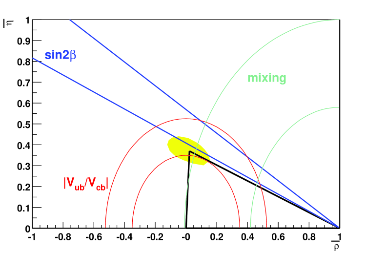
Figure 1: The 95% CL error ellipse for CKM parameters $\bar{\rho}$ and $\bar{\eta}$ together with the constraints on the Unitarity Triangle from mixing, $|V_{ub}/V_{cb}|$ and $\sin 2\beta$.

The theoretical branching ratios and contributions of the individual channels to $\chi^{2}$ based on these best fit values are given in table 8. The theoretical values shown use the $a_{i}$ coefficients listed in table 1 as model 2. These are the process-independent generalized factorization $a_{i}$ coefficients computed for the renormalization scale $\mu=m_{b}/2$. Also in the fit we take the electroweak penguin contribution to be $a_{9}=-0.0094-0.0002i$ [10]. Table 8 shows results with the systematic and statistical errors added in quadrature:$\sigma^{2}=\sigma^{2}_{{\rm stat}}+\sigma^{2}_{{\rm syst}}$. We have also done the computation using simple addition of errors $\sigma=\sigma_{{\rm stat}}+\sigma_{{\rm syst}}$. Both procedures are ad hoc, addition in quadrature reduces the influence of the systematic errors which are in general the smallest. The values of the best fit parameters $P_{2,i}$ are shown in table 9 together with our estimates of the two standard deviation errors. These errors are of course highly correlated. A plot of the error matrix ellipse for the Wolfenstein parameters $\bar{\rho}$ and $\bar{\eta}$ is shown in figure 1. The results in table 9 for the best fit values of the various form factors lie within the spread of theoretical estimates for these form factors (see tables 2 and 3).

6 Discussion and conclusions

We have investigated two-body charmless hadronic $B$ decays within the so called QCD factorization model, making use of simplifications which arise from working in the heavy quark limit. This is particularly evident for the $B\rightarrow VV$ processes which we argue to be predominantly of zero helicity. Consequently a wide range of decays can be expressed in terms of a relatively small number of soft QCD parameters, thus providing a theoretical framework which should be adequate to confront data for some time to come.

Different factorization models merely modify the $a_{i}$ coefficients which premultiply the various combinations of soft QCD parameters, thus allowing ready comparisons between these models.

If, in $B$ decays to two vector mesons, there is a significant contribution from the $\lambda=\pm$ helicity states, it should be apparent in the Dalitz type plots for the final decay products. Table 3 suggests that the negative helicity state might be important for $\bar{B}^{0}$ and $B^{-}$ decays, and the positive helicity state for $B^{0}$ and $B^{+}$ decays. Since each helicity contributes incoherently to the branching ratio, each helicity can be considered as a separate channel. The additional helicity channels can be included at the cost of extra soft QCD parameters. The only vector channels in table 8 are $B\rightarrow K^{*}\phi$ and in these channels there is some evidence [34] for contributions from non-zero helicities. It can be seen from tables 1, 6 and 7 that the zero helicity amplitudes (the only ones included) are proportional to $A_{K^{*}}$, a parameter which contributes significantly only to the $K^{*}\phi$ channels. Splitting the decay rates into the individual helicity channels will hardly effect the fit, it will only modify the estimate of $A_{K^{*}}$ given in table 9 and introduce more soft QCD parameters for the other helicities.

To economize in the number of soft QCD parameters we have not included decay channels involving $\eta$ and $\eta^{\prime}$ mesons. These amplitudes involve the mixing angle between the $(u\bar{u}+d\bar{d})$ and $s\bar{s}$ combinations. Also, in principle, there is mixing with $c\bar{c}$ which, though small, could make a significant contribution to decay modes through the enhanced quark decay modes $b\rightarrow cq\bar{c}$.

From table 8 it seems that of the nineteen channels included in the present analysis only the $PV$ channel $\pi^{-}K^{*0}$, and to a lesser extent $\pi^{-}K^{*+}$ and $\omega K^{0}$, give a large contribution to the overall $\chi^{2}$. The $\omega K^{0}$ channel has its largest theoretical contribution from the $b\rightarrow s$ penguin and, in particular, from the $a_{4}$ and $a_{6}$ terms. The theoretical branching ratio is small because of the cancellation, evident in tables 1 and 6, between these terms. It is difficult for the theory to explain a branching ratio greater than $2\times 10^{-6}$.

The $\pi^{-}K^{*0}$ channel is well measured, Belle gives a large branching ratio consistent with the BaBar result $(15.5\pm 3.4\pm 1.8)\times 10^{-6}$ shown in table 8, whereas the CLEO value is lower. It is interesting to compare this channel with $\pi^{-}K^{0}$, also well measured and with only a marginally larger branching ratio. A fit of the theoretical ratio

$$\frac{{\rm Br}(B\rightarrow\pi^{-}K^{0})}{{\rm Br}(B\rightarrow\pi^{-}K^{*0})} = \left(\frac{f_{K}}{f_{K^{*}}}\right)\left(1+R^{K}_{\chi}\frac{a_{6}}{a_{4}}\right)^{2}$$ (58)

$$\approx 0.547(1+1.3R^{K}_{\chi})^{2}$$

to the BaBar and Belle data implies $R^{K}_{\chi}\leq 0.5$. Our fit does agree well with the CLEO result.

References

Tables and table captions

Table 1: Decay amplitude coefficients $a_{i}$ in the matrix elements of the effective Hamiltonian (8) for several theoretical models. Model 1 is a simple tree plus QCD penguin as described in section 2, model 2 is generalized factorization with the effective Wilson coefficients evaluated at the renormalization scale $\mu=m_{b}/2$ and $q^{2}=m_{b}^{2}/4$ [35], and model 3 is QCD factorization at $\mu=m_{b}/2$ evaluated using the expressions of Beneke et al [14, 23]. The imaginary part of each coefficient is in parentheses.

Model $a_{1}^{u}$ $a_{2}^{u}$ $a_{3}^{u}=a_{3}^{c}$ $a_{4}^{u}$ $a_{4}^{c}$ 1 1.0000 0.3333 0.0000 $-$0.0492 $-$0.0524 ($-0.0234i$) ($-0.0059i$) 2 1.0523 0.0333 0.0062 $-$0.0397 $-$0.0496 ($-$0.0148i) ($-$0.0094i) 3 1.0510 0.0499 0.0050 $-$0.030 $-$0.038 (0.0335i) ($-$0.1063i) (0.0033i) ($-$0.019i) ($-$0.009i) $a_{5}^{u}=a_{5}^{c}$ $a_{6}^{u}$ $a_{6}^{c}$ 1 0.0000 $-$0.0492 $-$0.0524 ($-0.0234i$) ($-0.0059i$) 2 $-$0.0064 $-$0.0397 $-$0.0496 ($-$0.0148i) ($-$0.0094i) 3 0.0050 $-$0.050 $-$0.055 (0.0033i) ($-$0.017i) ($-$0.005i)

Table 2: Theoretical form factors for $B\rightarrow\pi$ and $B\rightarrow K$ transitions.

• Model	$F_{\pi}(0)$	$F_{K}(0)$
  Lattice QCDa	0.27
  Quark model wave functionsb	0.33
  Quark model wave functionsc		0.38
  Light cone sum ruled	0.305	0.341

• ^a Ref. [36]

• ^b Ref. [37]

• ^c Ref. [38]

• ^d Ref. [39]

Table 3: Theoretical form factors and helicity amplitudes for $\bar{B}^{0}\rightarrow\rho^{+}$ and $B^{-}\rightarrow K^{*-}$ transitions. It can be seen that, although the helicity zero channel for $B\rightarrow VV$ decays can be expected to dominate, this table shows that much cancellation is anticipated in (3). The extent to which the helicity zero states dominate should be apparent in Dalitz type plots for the final decay products.

Reference $A_{1}(0)$ $A_{2}(0)$ $V(0)$ $A_{0}(0)$ $|H_{+}(m_{V}^{2})|^{2}$ $|H_{-}(m_{V}^{2})|^{2}$ $|H_{0}(m_{V}^{2})|^{2}$ $\bar{B}^{0}\rightarrow\rho^{+}$ 1a 0.27 0.26 0.35 0.30 0.008 10.1 121 2b 0.26 0.22 0.34 0.38 0.006 9.4 185 3c 0.27 0.28 0.35 0.24 0.008 10.1 81 4d 0.30 0.33 0.37 0.21 0.034 11.9 66 5e 0.28 0.28 0.33 0.28 0.057 9.9 107 $B^{-}\rightarrow K^{*-}$ 2b 0.34 0.28 0.46 0.49 0.02 16.4 224 4d 0.36 0.40 0.45 0.26 0.10 17.1 75 6f 0.37 0.40 0.47 0.30 0.30 18.3 93 7g 0.33 0.33 0.37 0.32 0.22 13.0 110

a Ref. [36] b Ref. [41] c Ref. [42] d Ref. [43] e Ref. [37] f Ref. [40] g Ref. [38]

Table 4: Factorization matrix elements $\tilde{Q}_{i}(h_{1},h_{2})$ for $\bar{B}^{0}\rightarrow h_{1}h_{2}$ decays arising from $b\rightarrow dq\bar{q}$.

Decaya	$\tilde{Q}_{1}$	$\tilde{Q}_{2}$	$\tilde{Q}_{3}$	$\tilde{Q}_{4}$	$\tilde{Q}_{5}$	$\tilde{Q}_{6}$	$\tilde{Q}_{9}$
$\pi^{+}\pi^{-}$	$-F_{\pi}f_{\pi}$	0	0	$-F_{\pi}f_{\pi}$	0	$-R_{\chi}^{\pi}F_{\pi}f_{\pi}$	0
$\pi^{0}\pi^{0}$	0	$F_{\pi}f_{\pi}$	0	$-F_{\pi}f_{\pi}$	0	$-R_{\chi}^{\pi}F_{\pi}f_{\pi}$	$\frac{3F_{\pi}f_{\pi}}{2}$
$\rho^{+}\pi^{-}$	$A_{\rho}f_{\pi}$	0	0	$A_{\rho}f_{\pi}$	0	$-R_{\chi}^{\pi}A_{\rho}f_{\pi}$	0
$\rho^{0}\pi^{0}$	0	$-\frac{A_{\rho}f_{\pi}+F_{\pi}f_{\rho}}{2}$	0	$\frac{A_{\rho}f_{\pi}+F_{\pi}f_{\rho}}{2}$	0	$-R_{\chi}^{\pi}\frac{A_{\rho}f_{\pi}}{2}$	$-\frac{3(A_{\rho}f_{\pi}+F_{\pi}f_{\rho})}{4}$
$\pi^{+}\rho^{-}$	$F_{\pi}f_{\rho}$	0	0	$F_{\pi}f_{\rho}$	0	0	0
$\omega\pi^{0}$	0	$\frac{A_{\omega}f_{\pi}-F_{\pi}f_{\omega}}{2}$	$-F_{\pi}f_{\omega}$	$-\frac{A_{\omega}f_{\pi}+F_{\pi}f_{\omega}}{2}$	$-F_{\pi}f_{\omega}$	$R_{\chi}^{\pi}\frac{A_{\omega}f_{\pi}}{2}$	$\frac{3A_{\omega}f_{\pi}-F_{\pi}f_{\omega}}{4}$
$\rho^{+}\rho^{-}$	$A_{\rho}f_{\rho}$	0	0	$A_{\rho}f_{\rho}$	0	0	0
$\rho^{0}\rho^{0}$	0	$-A_{\rho}f_{\rho}$	0	$A_{\rho}f_{\rho}$	0	0	$-\frac{3A_{\rho}f_{\rho}}{2}$
$\omega\rho^{0}$	0	$\frac{A_{\omega}f_{\rho}-A_{\rho}f_{\omega}}{2}$	$-A_{\rho}f_{\omega}$	$-\frac{A_{\omega}f_{\rho}+A_{\rho}f_{\omega}}{2}$	$-A_{\rho}f_{\omega}$	0	$\frac{3A_{\omega}f_{\rho}-A_{\rho}f_{\omega}}{4}$
$\omega\omega$	0	$A_{\omega}f_{\omega}$	$2A_{\omega}f_{\omega}$	$A_{\omega}f_{\omega}$	$2A_{\omega}f_{\omega}$	0	$\frac{A_{\omega}f_{\omega}}{2}$
$\bar{K}^{0}K^{0}$	0	0	0	$-F_{K}f_{K}$	0	$-R_{\chi}^{K}F_{K}f_{K}$	0
$\bar{K}^{*0}K^{0}$	0	0	0	$A_{K^{*}}f_{K}$	0	$-R_{\chi}^{K}A_{K^{*}}f_{K}$	0
$\bar{K}^{0}K^{*0}$	0	0	0	$F_{K}f_{K^{*}}$	0	0	0
$\bar{K}^{*0}K^{*0}$	0	0	0	$A_{K^{*}}f_{K^{*}}$	0	0	0
$\phi\pi^{0}$	0	0	$\frac{F_{\pi}f_{\phi}}{\sqrt{2}}$	0	$\frac{F_{\pi}f_{\phi}}{\sqrt{2}}$	0	$-\frac{F_{\pi}f_{\phi}}{3\sqrt{2}}$

^a The decays to $\phi\rho^{0}$ and $\phi\omega$ are obtained from $\phi\pi^{0}$ by the substitutions $F_{\pi}\rightarrow A_{\rho}$ and $F_{\pi}\rightarrow-A_{\omega}$ respectively. The decays to $K^{+}K^{-},\;K^{+}K^{*-},\;K^{*+}K^{-}$ and $K^{*+}K^{*-}$ receive no contribution from $\tilde{Q}_{1,\ldots,6}$

Table 5: Factorization matrix elements $\tilde{Q}_{i}(h_{1},h_{2})$ for $B^{-}\rightarrow h_{1}h_{2}$ decays arising from $b\rightarrow dq\bar{q}$.

Decaya	$\tilde{Q}_{1}$	$\tilde{Q}_{2}$	$\tilde{Q}_{3}$	$\tilde{Q}_{4}$	$\tilde{Q}_{5}$	$\tilde{Q}_{6}$	$\tilde{Q}_{9}$
$\pi^{0}\pi^{-}$	$-\frac{F_{\pi}f_{\pi}}{\sqrt{2}}$	$-\frac{F_{\pi}f_{\pi}}{\sqrt{2}}$	0	0	0	0	$-\frac{3F_{\pi}f_{\pi}}{2\sqrt{2}}$
$\rho^{0}\pi^{-}$	$\frac{A_{\rho}f_{\pi}}{\sqrt{2}}$	$\frac{F_{\pi}f_{\rho}}{\sqrt{2}}$	0	$\frac{A_{\rho}f_{\pi}-F_{\pi}f_{\rho}}{\sqrt{2}}$	0	$-R_{\chi}^{\pi}\frac{A_{\rho}f_{\pi}}{\sqrt{2}}$	$\frac{3F_{\pi}f_{\rho}}{2\sqrt{2}}$
$\omega\pi^{-}$	$\frac{A_{\omega}f_{\pi}}{\sqrt{2}}$	$\frac{F_{\pi}f_{\omega}}{\sqrt{2}}$	$\sqrt{2}F_{\pi}f_{\omega}$	$\frac{A_{\omega}f_{\pi}+F_{\pi}f_{\omega}}{\sqrt{2}}$	$\sqrt{2}F_{\pi}f_{\omega}$	$-R_{\chi}^{\pi}\frac{A_{\omega}f_{\pi}}{\sqrt{2}}$	$\frac{F_{\pi}f_{\omega}}{2\sqrt{2}}$
$\pi^{0}\rho^{-}$	$\frac{F_{\pi}f_{\rho}}{\sqrt{2}}$	$\frac{A_{\rho}f_{\pi}}{\sqrt{2}}$	0	$\frac{F_{\pi}f_{\rho}-A_{\rho}f_{\pi}}{\sqrt{2}}$	0	$R_{\chi}^{\pi}\frac{A_{\rho}f_{\pi}}{\sqrt{2}}$	$\frac{3A_{\rho}f_{\pi}}{2\sqrt{2}}$
$\rho^{0}\rho^{-}$	$\frac{A_{\rho}f_{\rho}}{\sqrt{2}}$	$\frac{A_{\rho}f_{\rho}}{\sqrt{2}}$	0	0	0	0	$\frac{3A_{\rho}f_{\rho}}{2\sqrt{2}}$
$\omega\rho^{-}$	$\frac{A_{\omega}f_{\rho}}{\sqrt{2}}$	$\frac{A_{\rho}f_{\omega}}{\sqrt{2}}$	$\sqrt{2}A_{\rho}f_{\omega}$	$\frac{A_{\omega}f_{\rho}+A_{\rho}f_{\omega}}{\sqrt{2}}$	$\sqrt{2}A_{\rho}f_{\omega}$	0	$\frac{A_{\rho}f_{\omega}}{2\sqrt{2}}$
$K^{-}K^{0}$	0	0	0	$-F_{K}f_{K}$	0	$-R_{\chi}^{K}F_{K}f_{K}$	0
$K^{*-}K^{0}$	0	0	0	$A_{K^{*}}f_{K}$	0	$-R_{\chi}^{K}A_{K^{*}}f_{K}$	0
$K^{-}K^{*0}$	0	0	0	$F_{K}f_{K^{*}}$	0	0	0
$K^{*-}K^{*0}$	0	0	0	$A_{K^{*}}f_{K^{*}}$	0	0	0
$\phi\pi^{-}$	0	0	$F_{\pi}f_{\phi}$	0	$F_{\pi}f_{\phi}$	0	$-\frac{F_{\pi}f_{\phi}}{2}$

^a The decay to $\phi\rho^{-}$ is obtained from that to $\phi\pi^{-}$ by the substitution $F_{\pi}\rightarrow A_{\rho}$.

Table 6: Factorization matrix elements $\tilde{Q}_{i}(h_{1},h_{2})$ for $\bar{B}^{0}\rightarrow h_{1}h_{2}$ decays arising from $b\rightarrow sq\bar{q}$.

Decay	$\tilde{Q}_{1}$	$\tilde{Q}_{2}$	$\tilde{Q}_{3}$	$\tilde{Q}_{4}$	$\tilde{Q}_{5}$	$\tilde{Q}_{6}$	$\tilde{Q}_{9}$
$K^{-}\pi^{+}$	$-F_{\pi}f_{K}$	0	0	$-F_{\pi}f_{K}$	0	$-R_{\chi}^{K}F_{\pi}f_{K}$	0
$K^{*-}\pi^{+}$	$F_{\pi}f_{K^{*}}$	0	0	$F_{\pi}f_{K^{*}}$	0	0	0
$K^{-}\rho^{+}$	$A_{\rho}f_{K}$	0	0	$A_{\rho}f_{K}$	0	$-R_{\chi}^{K}A_{\rho}f_{K}$	0
$K^{*-}\rho^{+}$	$A_{\rho}f_{K^{*}}$	0	0	$A_{\rho}f_{K^{*}}$	0	0	0
$\bar{K}^{0}\pi^{0}$	0	$-\frac{F_{K}f_{\pi}}{\sqrt{2}}$	0	$\frac{F_{\pi}f_{K}}{\sqrt{2}}$	0	$R_{\chi}^{K}\frac{F_{\pi}f_{K}}{\sqrt{2}}$	$-\frac{3F_{K}f_{\pi}}{2\sqrt{2}}$
$\bar{K}^{*0}\pi^{0}$	0	$\frac{A_{K^{*}}f_{\pi}}{\sqrt{2}}$	0	$-\frac{F_{\pi}f_{K^{*}}}{\sqrt{2}}$	0	0	$\frac{3A_{K^{*}}f_{\pi}}{2\sqrt{2}}$
$\bar{K}^{0}\rho^{0}$	0	$\frac{F_{K}f_{\rho}}{\sqrt{2}}$	0	$-\frac{A_{\rho}f_{K}}{\sqrt{2}}$	0	$R_{\chi}^{K}\frac{A_{\rho}f_{K}}{\sqrt{2}}$	$\frac{3F_{K}f_{\rho}}{2\sqrt{2}}$
$\bar{K}^{*0}\rho^{0}$	0	$\frac{A_{K^{*}}f_{\rho}}{\sqrt{2}}$	0	$-\frac{A_{\rho}f_{K^{*}}}{\sqrt{2}}$	0	0	$\frac{3A_{K^{*}}f_{\rho}}{2\sqrt{2}}$
$\bar{K}^{0}\omega$	0	$\frac{F_{K}f_{\omega}}{\sqrt{2}}$	$\sqrt{2}F_{K}f_{\omega}$	$\frac{A_{\omega}f_{K}}{\sqrt{2}}$	$\sqrt{2}F_{K}f_{\omega}$	$-R_{\chi}^{K}\frac{A_{\omega}f_{K}}{\sqrt{2}}$	$\frac{F_{K}f_{\omega}}{2\sqrt{2}}$
$\bar{K}^{*0}\omega$	0	$\frac{A_{K^{*}}f_{\omega}}{\sqrt{2}}$	$\sqrt{2}A_{K^{*}}f_{\omega}$	$\frac{A_{\omega}f_{K^{*}}}{\sqrt{2}}$	$\sqrt{2}A_{K^{*}}f_{\omega}$	0	$\frac{A_{K^{*}}f_{\omega}}{2\sqrt{2}}$
$\bar{K}^{0}\phi$	0	0	$F_{K}f_{\phi}$	$F_{K}f_{\phi}$	$F_{K}f_{\phi}$	0	$-\frac{F_{K}f_{\phi}}{2}$
$\bar{K}^{*0}\phi$	0	0	$A_{K^{*}}f_{\phi}$	$A_{K^{*}}f_{\phi}$	$A_{K^{*}}f_{\phi}$	0	$-\frac{A_{K^{*}}f_{\phi}}{2}$

Table 7: Factorization matrix elements $\tilde{Q}_{i}(h_{1},h_{2})$ for $B^{-}\rightarrow h_{1}h_{2}$ decays arising from $b\rightarrow sq\bar{q}$.

Decay	$\tilde{Q}_{1}$	$\tilde{Q}_{2}$	$\tilde{Q}_{3}$	$\tilde{Q}_{4}$	$\tilde{Q}_{5}$	$\tilde{Q}_{6}$	$\tilde{Q}_{9}$
$\pi^{0}K^{-}$	$-\frac{F_{\pi}f_{K}}{\sqrt{2}}$	$-\frac{F_{K}f_{\pi}}{\sqrt{2}}$	0	$-\frac{F_{\pi}f_{K}}{\sqrt{2}}$	0	$-R_{\chi}^{K}\frac{F_{\pi}f_{K}}{\sqrt{2}}$	$-\frac{3F_{K}f_{\pi}}{2\sqrt{2}}$
$\pi^{0}K^{*-}$	$\frac{F_{\pi}f_{K^{*}}}{\sqrt{2}}$	$\frac{A_{K^{*}}f_{\pi}}{\sqrt{2}}$	0	$\frac{F_{\pi}f_{K^{*}}}{\sqrt{2}}$	0	0	$\frac{3A_{K^{*}}f_{\pi}}{2\sqrt{2}}$
$\pi^{-}\bar{K}^{0}$	0	0	0	$-F_{\pi}f_{K}$	0	$-R_{\chi}^{K}F_{\pi}f_{K}$	0
$\pi^{-}\bar{K}^{*0}$	0	0	0	$F_{\pi}f_{K^{*}}$	0	0	0
$\rho^{-}\bar{K}^{0}$	0	0	0	$A_{\rho}f_{K}$	0	$-R_{\chi}^{K}A_{\rho}f_{K}$	0
$\rho^{-}\bar{K}^{*0}$	0	0	0	$A_{\rho}f_{K^{*}}$	0	0	0
$\rho^{0}K^{-}$	$\frac{A_{\rho}f_{K}}{\sqrt{2}}$	$\frac{F_{K}f_{\rho}}{\sqrt{2}}$	0	$\frac{A_{\rho}f_{K}}{\sqrt{2}}$	0	$-R_{\chi}^{K}\frac{A_{\rho}f_{K}}{\sqrt{2}}$	$\frac{3F_{K}f_{\rho}}{2\sqrt{2}}$
$\rho^{0}K^{*-}$	$\frac{A_{\rho}f_{K^{*}}}{\sqrt{2}}$	$\frac{A_{K^{*}}f_{\rho}}{\sqrt{2}}$	0	$\frac{A_{\rho}f_{K^{*}}}{\sqrt{2}}$	0	0	$\frac{3A_{K^{*}}f_{\rho}}{2\sqrt{2}}$
$\omega K^{-}$	$\frac{A_{\omega}f_{K}}{\sqrt{2}}$	$\frac{F_{K}f_{\omega}}{\sqrt{2}}$	$\sqrt{2}F_{K}f_{\omega}$	$\frac{A_{\omega}f_{K}}{\sqrt{2}}$	$\sqrt{2}F_{K}f_{\omega}$	$-R_{\chi}^{K}\frac{A_{\omega}f_{K}}{\sqrt{2}}$	$\frac{F_{K}f_{\omega}}{2\sqrt{2}}$
$\omega K^{*-}$	$\frac{A_{\omega}f_{K^{*}}}{\sqrt{2}}$	$\frac{A_{K^{*}}f_{\omega}}{\sqrt{2}}$	$\sqrt{2}A_{K^{*}}f_{\omega}$	$\frac{A_{\omega}f_{K^{*}}}{\sqrt{2}}$	$\sqrt{2}A_{K^{*}}f_{\omega}$	0	$\frac{A_{K^{*}}f_{\omega}}{2\sqrt{2}}$
$\phi K^{-}$	0	0	$F_{K}f_{\phi}$	$F_{K}f_{\phi}$	$F_{K}f_{\phi}$	0	$-\frac{F_{K}f_{\phi}}{2}$
$\phi K^{*-}$	0	0	$A_{K^{*}}f_{\phi}$	$A_{K^{*}}f_{\phi}$	$A_{K^{*}}f_{\phi}$	0	$-\frac{A_{K^{*}}f_{\phi}}{2}$

Table 8: Measured branching ratio Br(exp), experimental error $\sigma$ (errors added in quadrature), theoretical branching ratio for best fit parameters Br(fit) and contribution to $\chi^{2}$ for various $B$ decay channels.

Decay	Br(exp)a	$\sigma^{a}$	Referenceb	Br(fit)a	$\chi^{2}$
$\pi^{+}\pi^{-}$	4.1	1.2	Ba1,Be1,Cl1	5.4	1.07
$\rho^{\pm}\pi^{\mp}$	28.9	6.9	Ba2,Be2,Cl1	29.6	0.01
$\rho^{0}\pi^{0}$	3.6	3.9	Ba2	0.1	0.15
$\omega\pi^{0}$	0.8	2.0	Ba3,Cl2	0.1	0.15
$\rho^{0}\pi^{-}$	10.4	3.9	Be2,Cl1	9.0	0.13
$\omega\pi^{-}$	6.6	2.2	Ba3,Cl2	7.15	0.06
$\pi^{0}K^{-}$	10.8	2.4	Ba1,Be1,Cl1	11.1	0.02
$\pi^{-}K^{0}$	18.2	3.9	Ba1,Be1, Cl1	18.1	0.00
$\pi^{-}K^{*0}$	15.9	3.7	Ba4,Be3,Cl2	5.0	8.75
$\omega K^{-}$	3.2	2.2	Cl2	1.4	0.68
$\phi K^{-}$	7.7	1.8	Ba5,Be2,Cl1	7.8	0.00
$\phi K^{*-}$	9.6	4.4	Ba5, Cl1	9.6	0.00
$\pi^{-}K^{+}$	16.7	2.2	Ba1, Be1,Cl1	16.9	0.01
$\pi^{-}K^{*+}$	22	11	Cl2	5.0	2.39
$\pi^{0}K^{0}$	8.2	3.3	Ba1,Be1,Cl1	6.7	0.20
$\pi^{0}K^{*0}$	2.1	2.1	Cl2	1.4	0.12
$\omega K^{0}$	10	6	Cl2	0.7	2.42
$\phi K^{0}$	8.1	3.2	Ba5	7.4	0.05
$\phi K^{*0}$	8.6	3.0	Ba5, Be2, Cl1	9.0	0.02

^a In units of $10^{-6}$.
^b References to experimental groups are: BaBar Ba1 Ref. [44], Ba2 Ref. [45], Ba3 Ref. [46], Ba4 Ref. [47], Ba5 Ref. [4]; Belle Be1 Ref. [48], Be2 Ref. [49], Be3 Ref. [50] and CLEO Cl1 Ref. [51], Cl2 Ref. [52].

Table 9: Best fit values and one-standard deviation errors of fitting parameters.

$F_{\pi}$	$F_{K}$	$A_{\rho}$	$A_{\omega}$	$A_{K^{*}}$
$0.243\pm 0.031$	$0.312\pm 0.040$	$0.404\pm 0.087$	$0.377\pm 0.067$	$0.349\pm 0.052$
$R^{\pi}_{\chi}$	$R^{K}_{\chi}$	$A$	$\bar{\eta}$	$\bar{\rho}$
$0.970\pm 0.000$	$1.200\pm 0.186$	$0.803\pm 0.063$	$0.375\pm 0.053$	$0.038\pm 0.104$

Figure captions

=0.9

References

- [1] CLEO Collaboration, Cronin-Henessy D et al2000 Phys. Rev. Lett. 85, 515–9 CLEO Collaboration, Jessop C P et al2000 Phys. Rev. Lett. 85 2881–5
- [2] Harrison P F and Quinn H R 1998 The BaBar Physics Book SLAC report SLAC-R-504 October 1998 BaBar Collaboration, Aubert B et al2001 Phys. Rev. Lett. 86 2515–22
- [3] BaBar Collaboration, Aubert B et al2001 Phys. Rev. Lett. 87 091801
- [4] BaBar Collaboration, Aubert B et al2001 Phys. Rev. Lett. 87 151801
- [5] Belle Collaboration, Abashian A et al2001 Phys. Rev. Lett. 86 2509–14 Belle Collaboration, Abe K et al2001 Phys. Rev. Lett. 87 101801
- [6] Belle Collaboration, Abe K et al2001 Phys. Rev. Lett. 87 091802
- [7] Buchalla G, Buras A J and Lautenbacher M E 1996 Rev. Mod. Phys. 68 1125–244
- [8] Feynman R P 1965 Symmetries in Particle Physics, ed A Zichichi (New York: Academic Press) p 167 Haan O and Stech B 1970 Nucl. Phys. B22 448–60 Ellis J, Gaillard M K and Nanopolous D V 1975 Nucl. Phys. B100 313–28 Fakirov D and Stech B 1978 Nucl. Phys. B133 315–26 Bauer M and Stech B 1980 Phys. Lett. B152 380–4
- [9] Ali A and Greub C 1998 Phys. Rev. D 57 2996–3016
- [10] Ali A, Kramer G and Lü C-D 1998 Phys. Rev. D 58 094009 Ali A, Kramer G and Lü C-D 1999 Phys. Rev. D 59 014005
- [11] Cheng H-Y and Tseng B 1998 Phys. Rev. D 58 094005
- [12] Cheng H-Y and Yang K C 2000 Phys. Rev. D 62 054029
- [13] Bander M, Silverman D and Soni A 1979 Phys. Rev. Lett. 43 242–5
- [14] Beneke M, Buchalla G, Neubert M and Sachrajda C T 1999 Phys. Rev. Lett. 83 1914–7
- [15] Beneke M, Buchalla G, Neubert M and Sachrajda C T 2000 Nucl. Phys. B 591 313–418 Beneke M, Buchalla G, Neubert M and Sachrajda C T 2000 hep-ph/0007256 (To appear in Proceedings of ICHEP2000, Osaka, Japan) Beneke M 2002 hep-ph/0207228
- [16] Beneke M 2001 J. Phys. G: Nucl. Part. Phys. 27 1069–80
- [17] Neubert M 2000 hep-ph/0006265 Neubert M 2000 hep-ph/0008072 Neubert M 2001 Nucl. Phys. Proc. Suppl. 99 113–20 Neubert M 2002 hep-ph/0207327
- [18] Du D, Yang D and Zhu G 2000 Phys. Lett. B488 46–54 Du D, Yang D and Zhu G 2000 hep-ph/0008216 Du D, Yang D and Zhu G 2001 Phys. Rev. D 64 014036
- [19] Yang M Z and Yang Y D 2000 Phys. Rev. D 62 114019 Du D, Gong H, Sun J, Yang D and Zhu G 2002 Phys. Rev. D 65 094025
- [20] Muta T, Sugamoto A, Yang M and Yang Y 2000 Phys. Rev. D 62 094020
- [21] Cheng H-Y and Yang K-C 2001 Phys. Lett. B511 40–8
- [22] Cheng H-Y and Yang K-C 2001 Phys. Rev. D 64 074004
- [23] Beneke M, Buchalla G, Neubert M and Sachrajda C T 2001 Nucl. Phys. B 606 245–321
- [24] Du D, Gong H, Sun J, Yang D and Zhu G Phys. Rev. D 65 074001
- [25] Bander M, Silverman D and Soni S 1979 Phys. Rev. Lett. 43 242–5
- [26] Szczepaniak A, Henley E M and Brodsky S J 1990 Phys. Lett. B243 287–92 Li H-n and Yu H L 1995 Phys. Rev. Lett. 74 4388–91 Li H-n and Yu H L 1996 Phys. Lett. B353 301–5 Li H-n and Yu H L 1996 Phys. Rev. D 53 2480–90 Chang C H and Li H-n 1997 Phys. Rev. D 55 5577–80 Keum Y Y, Li H-n and Sanda A I 2001 Phys. Lett. B504 6–14 Keum Y Y, Li H-n and Sanda A I 2001 Phys. Rev. D 63 054008 Keum Y Y and Li H-n 2001 Phys. Rev. D 63 074006 Lü C D, Ukai K and Yang M Z 2001 Phys. Rev. D 074009
- [27] Descotes-Genon S and Sachrajda C T 2001 hep-ph/0109260 Neubert M 2001 hep-ph/0110301 Quinn H 2001 hep-ph/0111169
- [28] Quinn H 2001 hep-ph/0111177
- [29] Ciuchini M, Franco E, Martinelli G, Pierini M and Silvestrini L 2001 Phys. Lett. B515 33 –41 Ciuchini M, Franco E, Martinelli G, Pierini M and Silvestrini L 2001 hep-ph/0110022 Ciuchini M, Franco E, Martinelli G, Pierini M and Silvestrini L 2002 hep-ph/0208048
- [30] Ciuchini et al2001 J. High Energy Phys. 0107 013
- [31] Abel S A, Cottingham W N and Whittingham I B 1998 Phys. Rev. D 58 073006
- [32] CLEO Collaboration, Behrens B H et al2000 Phys. Rev. D 61 052001
- [33] James F and Roos M, MINUIT, CERN D506, CERN Program Library Office, CERN, CH-1211 Geneva 23, Switzerland
- [34] BaBar Collaboration, Aubert B et al2001 hep-ex/0107049
- [35] Cottingham W N, Mehrban H and Whittingham I B 1999 Phys. Rev. D 60 114029
- [36] UKQCD Collaboration, Del Debbio L et al1998 Phys. Lett. B416 392–401
- [37] Wirbel M, Stech B and Bauer M 1985 Z. Phys. C 29 637–42
- [38] Bauer M, Stech B and Wirbel M 1987 Z. Phys. C 34 103–15
- [39] Ball P 1998 J. High Energy Phys. 09 005
- [40] Colangelo P, De Fazio F, Santorelli P and Scrimieri E 1996 Phys. Rev. D 53 3672–86
- [41] Ball P and Braun V M 1998 Phys. Rev. D 58 094016
- [42] Ball P and Braun V M 1997 Phys. Rev. D 55 5561–76
- [43] Aliev T M, Savci M and Özpineci A 1997 Phys. Rev. D 56 4260–7
- [44] BaBar Collaboration, Cavoto G 2001 hep-ex/0105018
- [45] BaBar Collaboration, Aubert B et al2001 hep-ex/0107058
- [46] BaBar Collaboration, Aubert, B et al2001 hep-ex/0108017
- [47] BaBar Collaboration, Aubert B et al2001 hep-ex/0109007
- [48] Belle Collaboration, Iijima T 2001 hep-ex/0105005
- [49] Belle Collaboration, Bozek A 2001 hep-ex/0104041
- [50] Belle Collaboration, Abe K et al2001 hep-ex/0107051
- [51] CLEO Collaboration, Gao Y 2001 hep-ex/0108005
- [52] CLEO Collaboration, Jessop C et alhep-ex/0006008