hep-ph/0101330

CERN-TH/2001-021

TTP01-05

The determination of $V_{ub}$ from inclusive semileptonic $B$ decays

Marek Jeżabek^1,2, Thomas Mannel^3,4,
Boris Postler³, Piotr Urban¹

¹Institute of Nuclear Physics, ul. Kawiory 26a,
PL-30055 Cracow, Poland.
²Institute of Physics, University of Silesia, ul. Uniwersytecka 4,
PL-40007 Katowice, Poland.
³Institut für Theoretische Teilchenphysik,
Universität Karlsruhe,
D – 76128 Karlsruhe, Germany.
⁴CERN-TH, CH-1211 Geneva 23, Switzerland.

The hadronic mass distribution in semileptonic $B$-meson decays can be used for extracting the charmless part and thus determining the $|V_{ub}/V_{cb}|$ ratio. We take into account first-order perturbative as well as non-perturbative QCD corrections. The sensitivity to model assumptions is studied and an estimate of the remaining uncertainties is performed.

1 Introduction

The CKM matrix element $V_{ub}$ plays an important role in the determination of the unitarity triangle. The cleanest method to obtain the absolute value $|V_{ub}|$ is through the measurement of semileptonic $b\to u$ transitions, which will eventually give the length of one of the sides of the unitarity triangle.

The possibilities of determining $V_{ub}$ from semileptonic decays have been studied in detail in the BaBar Workshop [1]. Here the conclusion was reached that the determination of $V_{ub}$ will be performed by a mixture of different methods.

One of the theoretically cleanest possibilities is to use inclusive semileptonic decays. Placing a cut on the hadronic invariant mass of the final state can in principle eliminate the charm contribution, which otherwise would be overwhelming. This cut on the hadronic invariant mass can be implemented at the asymmetric $B$ factories, making this method experimentally feasible.

From the theoretical side the decay rate, including cuts on the lepton energy as well as on the hadronic invariant mass of the final state, can be computed systematically within the framework of the $1/m_{b}$ expansion, except for certain regions of phase space, where the $1/m_{b}$ expansion has to be replaced by an expansion in twist. To describe these regions of phases space one has to introduce a so-called “shape function”, which in principle introduces a large hadronic uncertainty.

Another method that has been proposed [2] avoids the twist expansion and relies only on a standard $1/m_{Q}$ expansion. This method needs a measurement of the lepton invariant mass spectrum, in which the regions of phase space where the shape function plays a role are kinematically suppressed. This method will also allow a clean determination of $V_{ub}$.

An alternative approach has been put forth in [3, 4] where the factorization into soft, jet and hard sub-processes [5] has been employed to relate the radiative $b$ decays to the semileptonic ones in a way which explicitly reduces the impact of the shape function uncertainties. Then a prediction of the ratio $|V_{ub}/V_{ts}|$ can be obtained with a good accuracy in a model independent way. This approach is similar to the one in [6].

Exclusive decays will open a completely different window on $V_{ub}$; however, in these decays a certain model dependence seems to be unavoidable, unless lattice data become reasonably precise.

From this variety of methods to determine $|V_{ub}|/|V_{cb}|$, we shall expand in this paper on the one in which a cut is applied on the hadronic invariant mass in semileptonic $B$ decays to filter out the $b\to u$ transitions. The advantage is that the hadronic invariant mass may be easier to measure, however, this method involves the shape function and potentially has larger theoretical uncertainties than the inclusive method using the leptonic invariant mass.The method based on the hadronic invariant mass spectrum has already been discussed in [7], where the main focus was on the perturbative contributions of order $\alpha_{s}$ and $\beta_{0}\alpha_{s}^{2}$.

The purpose of this paper is to consider this approach in detail and to try to estimate the uncertainties, including perturbative as well as non-perturbative contributions and, in addition, a cut on the lepton energy. It turns out that the main uncertainties originate from the heavy quark mass $m_{b}$ (or, equivalently, from $\bar{\Lambda}=M_{B}-m_{b}$ where $M_{B}$ is the $B$-meson mass) and the strong coupling $\alpha_{s}$, while the uncertainties introduced by the shape function are small.

The next section deals with the kinematics. Then, in Section 3, we give the radiative corrections for the partonic process $b\to u\ell\bar{\nu}_{\ell}$ to order $\alpha_{s}$. In section 4 we include the leading-twist non-perturbative effects; this requires the introduction of the light-cone distribution function for the heavy quark, for which we use a simple parametrization. We combine the perturbative and non-perturbative corrections and study the uncertainties in the determination of $|V_{ub}|/|V_{cb}|$ in section 5.

2 Kinematical Relations and Definitions

We shall first define the kinematic variables for the partonic process $b\rightarrow u\ell\bar{\nu_{\ell}}$. Although we also use results for the semileptonic $b\rightarrow c$ decay rate, the latter is considered in the partonic framework solely. In fact, we only need the total rate with a single lower cut on the electron energy for $b\rightarrow c$; we thus refer the reader to [8] for further discussion of the kinematics of this process. The initial state $b$ quark has a momentum $p_{b}=m_{b}v$, where $v$ is the velocity of the $B$ meson. With the momentum transfer to the leptons $q=k+k^{\prime}$ the variable $p=q-m_{b}v$ is the partonic momentum of the final state. Writing $E_{\ell}=vk$ for the energy of the lepton, $E_{p}=vp$ for the partonic energy of the final state and $p^{2}$ for the partonic invariant mass, we define the following re-scaled variables

$$x=\frac{2E_{\ell}}{m_{b}}\,,\qquad x_{p}=\frac{2E_{p}}{m_{b}}\,,\qquad y=\frac{q^{2}}{m_{b}^{2}}\,,\qquad z=\frac{p^{2}}{m_{b}^{2}}\,.$$ (1)

One of these variables is superfluous when calculating the triple differential decay rate and can be substituted by using the relation

$$x_{p}+y-z=1\,.$$ (2)

Using these definitions, we compute the triple differential partonic rate to order $\alpha_{s}$ and order $1/m_{b}$, and split it into the tree-level term $\Gamma^{0}$ and the ${\cal O}(\alpha_{s})$ correction $\Gamma^{1}$:

$$\mbox{d}\Gamma^{pert}=\mbox{d}\Gamma^{parton,0}+\frac{2\alpha_{s}}{3\pi}\mbox{d}\Gamma^{pert,1}\,.$$ (3)

The radiative corrections to ${\cal O}(\alpha_{s})$ have recently been calculated by [9]; we have checked their result and find full agreement with ours. The formulae up to terms ${\cal O}(\alpha_{s})$ are quite tedious and can be found in [9]. However, we present them in the Appendix in a form suitable for our numerical evaluation.

We shall now discuss the hadronic kinematics. The momentum of the initial $B$ meson is $M_{B}v=(m_{b}+\bar{\Lambda})v$, where we have used the relation between the $B$ meson and the $b$-quark mass

$$M_{B}=m_{b}+\bar{\Lambda}$$ (4)

which holds to leading order in the $1/m_{b}$ expansion. Consequently, the hadronic mass of the final state is $M_{X}^{2}=(M_{B}v-q)^{2}=(p+\bar{\Lambda}v)^{2}=p^{2}+2E_{p}\bar{\Lambda}+\bar{\Lambda}^{2}$ and hence involves both the partonic invariant mass and the partonic energy. Thus we have

$$\frac{\mbox{d}\Gamma^{parton}}{\mbox{d}M_{X}^{2}\mbox{d}E_{l}}(m_{b}) = \int\limits_{0}^{1}\mbox{d}x\int\limits_{1-x}^{2-x}\mbox{d}x_{p}\int\limits_{z_{min}}^{z_{max}}\mbox{d}z\frac{\mbox{d}^{3}\Gamma^{pert}}{\mbox{d}x\mbox{d}x_{p}\mbox{d}z}\times$$ (5)

$$\delta(M_{X}^{2}-m_{b}^{2}z-x_{p}\bar{\Lambda}m_{b}-\bar{\Lambda}^{2})\delta\left(E_{l}-\frac{m_{b}x}{2}\right)\,.$$

where the kinematic limits of the $z$ integration depend on the cuts as well as on $x_{p}$. They are

$$z_{min}=\left\{\begin{array}[]{ll}0&\mbox{for }x_{p}\leq 1\,,\\ x_{p}-1&\mbox{for }x_{p}>1\,,\end{array}\right.$$ (8)

and

$$z_{max}=(1-x)(x_{p}+x-1)\,.$$ (9)

3 Perturbative corrections

The analysis we perform requires the knowledge of the triple differential partonic rate to order $\alpha_{s}$, as can already be seen from Eq. (5) as well as from the final formula, Eq. (14). The Born approximation is proportional to the delta function of argument $z$,

$$\frac{\mbox{d}^{3}\Gamma^{pert,0}}{\mbox{d}x\,\mbox{d}x_{p}\,\mbox{d}z}=12\Gamma_{0}\,(2-x-x_{p})(x+x_{p}-1)\delta(z),$$ (10)

where

$$\Gamma_{0}=\frac{G_{F}^{2}m_{b}^{5}}{192\pi^{3}}.$$ (11)

As is well known, the virtual one-loop correction contains an infrared divergence that cancels with the real gluon emission. We shall discuss in the next section how to include the leading-twist non-perturbative effects by “smearing” over some small window in the hadronic invariant mass. While choosing an excessively small value for this window would still yield a meaningless result, a region of size $\bar{\Lambda}m_{b}$ is believed to exist, where this smearing provides a realistic approximation. Instead of keeping track of the virtual and real parts, one can now use an appropriately integrated distribution, which is subjected to the smearing procedure. The tree-level term is rather simple to implement numerically but, on the other hand, we have found it very useful to perform one integration of the one-loop correction analytically. On inspection of Eq. (14) in conjunction with Eq. (5), it is clear that the following integral is of use:

$$F(x,x_{p},z)=\int_{z_{min}}^{z}\mbox{d}z^{\prime}\frac{\mbox{d}\Gamma^{pert,1}}{\Gamma_{0}\,\mbox{d}x\mbox{d}x_{p}\mbox{d}z^{\prime}}.$$ (12)

This function is a lengthy and tedious expression, and it is given in the Appendix.

4 Leading-twist non-perturbative corrections

It has been shown that the leading-twist non-perturbative corrections can be implemented at tree level by redefining the heavy-quark mass and a subsequent convolution with a so-called shape function [10, 11, 12, 13, 14]. This convolution corresponds to an integration over the light-cone variable $k_{+}$, namely

$$\mbox{d}\Gamma^{hadron}=\int\limits^{\bar{\Lambda}}_{-m_{b}}\mbox{d}\Gamma^{parton}(m_{b}+k_{+})\,f(k_{+})\,\mbox{d}k_{+}$$ (13)

in $\mbox{d}\Gamma^{HQET}$. Although this formula is quite suggestive [15], it has been shown recently that it contains,in fact, spurious contributions of sub-leading twist [16]. Furthermore, once radiative corrections are implemented, this simple convolution formula will probably no longer hold [17]. However, there is no fully consistent way yet to include radiative corrections into this convolution, and hence we proceed in a naive way as suggested in [15].

This naive way is to actually use the convolution formula (13) also beyond tree level, which is at least as consistent as using the ACCMM model [18] beyond tree level, which is common practice. In fact, the connection between the ACCMM model and the shape function formalism has been pointed out in [19].

It is convenient to change the variable of integration according to

$$\mbox{d}\Gamma^{hadron}=\int\limits^{M_{B}}_{0}\mbox{d}\Gamma^{parton}(m^{*})\,f(m^{*})\,\mbox{d}m^{*}$$ (14)

with $m^{*}=m_{b}+k_{+}$.

The shape function is a nonperturbative function which has to be determined either from experiment or by some model. A few relations are known for the moments of the shape function $\langle k_{+}^{n}\rangle$:

$$\langle k_{+}^{0}\rangle=1\,,\quad\langle k_{+}^{1}\rangle=0\quad\mbox{and}\quad\langle k_{+}^{2}\rangle=-\frac{1}{3}\lambda_{1}\quad$$ (15)

For our study we shall use an ansatz for the shape function. Taking a simple three parameter function [20]

$$f(x)=N\,\mbox{e}^{c\,x}\,(1-x)^{a}\,,\quad x=1-\frac{M_{B}-m^{*}}{\bar{\Lambda}}\,,$$ (16)

we can express the parameters of this ansatz in terms of the HQET parameters (15)

$$N=\frac{c^{c}}{\bar{\Lambda}\mbox{e}^{c}\Gamma(c)},\quad a=c-1,\quad c=-\frac{3\bar{\Lambda}^{2}}{\lambda_{1}}\,.$$ (17)

We shall discuss the dependence of our results on this ansatz in the next section.

5 The measurement of $|V_{ub}|$

For the measurement of $|V_{ub}|$ we propose to study semileptonic $B$ decays with certain cuts. The first cut is on the lepton energy $E_{l}$, which is mainly given by the experimental limitations on detecting electrons with small momenta. The second cut is on the hadronic invariant mass $M_{X}$ of the final state, which serves to suppress charm. We define the semileptonic rates including cuts as

$$\Gamma(M_{cut}^{2},E_{cut})=\int\limits_{0}^{M_{cut}^{2}}\mbox{d}M_{X}^{2}\int\limits_{E_{cut}}^{\frac{M^{2}_{B}-M_{X}^{2}}{2\,M_{B}}}\mbox{d}E_{l}\,\frac{\mbox{d}\Gamma(B\rightarrow X_{u}e\bar{\nu_{e}})}{\mbox{d}M_{X}^{2}\mbox{d}E_{l}},$$ (18)

Clearly the region $0<M_{X}<M_{D}$ is dominated by $b\to u$ transitions, and we thus use in this region the expressions for $b\to u$ decays only.

We shall normalize everything to the rate with no cut on the hadronic invariant mass, and thus obtain, for the ratio $r$:

$$\frac{|V_{ub}|^{2}}{|V_{cb}|^{2}}r=\frac{\Gamma(M_{cut}^{2},E_{cut})}{\Gamma(M_{B},E_{cut})},$$ (19)

where in the denominator we can safely take into account the $b\to c$ channel only, the $b\to u$ contribution being only about 1%.

For the charmless decay rate entering the numerator, we include the results discussed above. The perturbative corrections are taken into account to one loop [8], while the non-perturbative ones are included to leading twist. The $b\to c$ decay rate in the denominator is evaluated including ${\cal O}(\alpha_{s})$ corrections.

Unlike the approach advertised in [2] and [21], the shape of the hadronic invariant mass spectrum depends on the shape function, for which we use the parametrization (16). However, as it will turn out, the precise form of the shape function is irrelevant for the ratio (19), the main sources of uncertainties are the value of the strong coupling and that of the quark masses. The latter may be replaced by $\bar{\Lambda}$, we thus use $m_{b}=\overline{M}_{B}-\bar{\Lambda}$ and $m_{c}=\overline{M}_{D}-\bar{\Lambda}$, where $\overline{M}$ denotes the spin-averaged meson mass.

The dependence on the shape function can be studied by checking the sensitivity of our result with respect to higher moments of this function. Since we have not included any $1/m_{b}^{2}$ terms in our calculation the ratio (19) should be reasonably insensitive already to the second moment of the shape function, which is given in terms of the kinetic energy operator $\lambda_{1}$ in (15). This forces us to make $M_{cut}$ as large as possible.

We have examined the ratio defined in Eq. (19), allowing the variations $0.4\mbox{ GeV}\leq\bar{\Lambda}\leq 0.75\mbox{ GeV}$, $0.2\leq\alpha_{s}\leq 0.3$ and $-0.6\mbox{ GeV}^{2}\leq\lambda_{1}\leq-0.1\mbox{ GeV}^{2}$.

Figure 1: Ratio $r$ as a function of the hadronic mass cut, with (dark) or without (light) correlation between the strong coupling constant and the pole mass

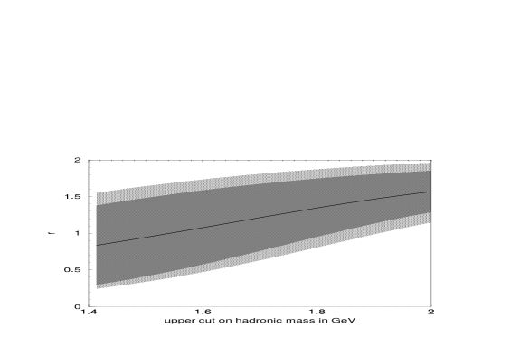
The main uncertainty is induced by $\alpha_{s}$ and $\bar{\Lambda}$, where $\bar{\Lambda}$ is equivalent to the heavy quark mass. It has been argued that these two quantities are correlated; the size of the radiative corrections depends on the particular choice of the mass.

Using the pole mass scheme, it has been shown that the radiative corrections are large and the perturbation series converges very slowly. Treating both the pole mass and the perturbative contributions independently, the uncertainties of the quantities would simply add, leaving us with a large (and certainly overestimated) uncertainty. In this case we get (see the lighter band in Fig. 1):

$$1.15\leq r\leq 1.96\quad\mbox{at }M^{2}_{cut}=4\mbox{ GeV}^{2}$$ (20)

where we have used $m_{b}^{pole}=(4.75\pm 0.15)$ GeV and $\alpha_{s}$ between 0.2 and 0.3. In this way we obtain a theoretical uncertainty of $25\%$ in the determination of the ratio.

Another option is to switch to a short-distance mass definition, such as $m_{b}^{\overline{MS}}$ by replacing

$$m_{b}^{pole}=m_{b}^{\overline{MS}}\left(1+\frac{4}{3\pi}\alpha_{s}\right),$$ (21)

which reduces the size of the coefficients of the perturbation series, and the pertrubative uncertainties thus become smaller. Using a recent value for $M_{b}^{\overline{MS}}$ [21]

$$m_{b}^{\overline{MS}}=(4.25\pm 0.08)\mbox{GeV},$$ (22)

we arrive at an estimate for $r$ with a smaller uncertainty (the darker band in Fig. 1)

$$1.28\leq r\leq 1.85\quad\mbox{at }M^{2}_{cut}=4\mbox{ GeV}^{2}.$$ (23)

In order to display the dependence on the input parameters, we choose the “average” values of the three parameters:

$$\bar{\Lambda}^{aver}=0.55\mbox{ GeV},\qquad\alpha_{s}^{aver}=0.25,\qquad\lambda_{1}^{aver}=-0.35\mbox{ GeV}^{2},$$ (24)

and obtain up to linear terms in the variations

$$r=1.58-0.86\frac{\Delta\bar{\Lambda}}{\bar{\Lambda}^{aver}}-0.26\frac{\Delta\alpha_{s}}{\alpha_{s}^{aver}}+0.06\frac{\Delta\lambda_{1}}{\lambda_{1}^{aver}}.$$ (25)

This explicitly shows that the dependence on $\lambda_{1}$, which is the second moment of the shape function, is weak. The dependence on even higher moments is expected to be further suppressed by inverse powers of the heavy quark mass.

In conclusion, our best estimate for $r$ is

$$r=1.57\pm 0.3\quad,$$ (26)

which corresponds to a theoretical uncertainty in the determination of $|V_{ub}/V_{cb}|$ of about ten percent

$$\left(\frac{\Delta|V_{ub}/V_{cb}|}{|V_{ub}/V_{cb}|}\right)_{theor}\approx 10\%$$ (27)

6 Conclusions

We have performed a detailed analysis of one of the possibilities to obtain $V_{ub}$ from inclusive semileptonic $B$ decays by placing a cut on the hadronic invariant mass to get rid of the charm background. This method has been criticized since it depends on the shape function, which describes the endpoint of the hadronic invariant mass spectrum. This function is not very well known and hence it has to be modelled, which will introduce some systematic uncertainty. However, integrating over the window in hadronic invariant masses relevant to $b\to u$ transitions, we have shown that the dependence on the shape function is much smaller than the uncertainties induced by the quark mass and by the truncation of the perturbative series.

The the ratio between the semileptonic rates including a cut on the hadronic invariant mass and the semileptonic rate without a cut yields $|V_{ub}/V_{cb}|$ up to a quantity $r$, which we have computed in leading twist approximation and to order $\alpha_{s}$. Based on our calculations the uncertainty in this quantity is $20\%$ leaving us with a $10\%$ theoretical uncertainty in the determination of $V_{ub}$. This method is thus one of the cleanest possible to obtain $V_{ub}$ at the ongoing $B$-factory experiments.

Appendix

We present here the convoluted spectra in some more detail, showing in particular a convenient way of calculating the contribution from the terms proportional to $\alpha_{s}$. The convolution of the partonic spectra results in the leading-twist approximated rate of $B\rightarrow X_{u}l\bar{\nu}$ decay. The resulting distribution can be written in the following form:

$$\frac{\mbox{d}\Gamma}{\mbox{d}M_{X}^{2}\mbox{d}E_{l}} = \int_{0}^{1}\mbox{d}x\int_{1-x}^{2-x}\mbox{d}x_{p}\int_{z_{min}}^{z_{max}}\mbox{d}z\int_{-\infty}^{M_{B}}\mbox{d}m^{*}f(m^{*})\frac{\mbox{d}\Gamma^{parton}}{\mbox{d}x\mbox{d}x_{p}\mbox{d}z}\times$$ (A.1)

$$\delta(M_{X}^{2}-m^{*2}z-x_{p}\bar{\Lambda}^{*}m^{*}-\bar{\Lambda}^{*2})\delta(E_{l}-\frac{m^{*}x}{2}).$$

The partonic rate can be split into the tree level term and the ${\cal O}(\alpha_{s})$ correction,

$$\mbox{d}\Gamma^{parton}=\mbox{d}\Gamma^{parton,0}+\frac{2\alpha_{s}}{3\pi}\mbox{d}\Gamma^{parton,1},$$ (A.2)

and the convoluted rate can then be divided up accordingly. Using the delta functions, the integrations involved in these rates can be simplified, yielding

$$\int_{E_{cut}}^{M_{B}/2}\mbox{d}E_{l}\int_{0}^{M_{cut}^{2}}\mbox{d}M_{X}^{2}\frac{\mbox{d}\Gamma^{(0)}(B\rightarrow X_{u}e\bar{\nu_{e}})}{\mbox{d}M_{X}^{2}\mbox{d}E_{l}}=$$

$$\int_{E_{cut}}^{M_{B}/2}\mbox{d}E_{l}\int_{2E_{l}/M_{B}}^{1}\mbox{d}x\int_{y_{min}}^{x}\mbox{d}y\,\frac{2}{x}f\left(\frac{2E_{l}}{x}\right)\frac{\mbox{d}\Gamma^{parton,0}}{\mbox{d}x\mbox{d}y},$$ (A.3)

$$y_{min}=\max\left\{0,\frac{1-M_{cut}^{2}-(M_{B}-2E_{l}/x)^{2}}{(2E_{l}/x)(M_{B}-2E_{l}/x)}\right\}$$ (A.4)

for the tree-level contribution, while the $\alpha_{s}$ correction contributes

$$\int_{E_{cut}}^{M_{B}/2}\mbox{d}E_{l}\int_{0}^{M_{cut}^{2}}\mbox{d}M_{X}^{2}\frac{\mbox{d}\Gamma^{(1)}(B\rightarrow X_{u}e\bar{\nu_{e}})}{\mbox{d}M_{X}^{2}\mbox{d}E_{l}}=$$

$$\int_{E_{cut}}^{M_{B}/2}\mbox{d}E_{l}\int_{2E_{l}/M_{B}}^{1}\mbox{d}x\int_{1-x}^{2-x}\mbox{d}x_{p}\int_{z_{min}}^{z_{max}}\mbox{d}z\,\frac{2}{x}f\left(\frac{2E_{l}}{x}\right)\frac{\mbox{d}\Gamma^{parton,1}}{\mbox{d}x\mbox{d}x_{p}\mbox{d}z},$$ (A.5)

where

$$z_{min}=\left\{\begin{array}[]{cc}0,&{\mbox{f}or\ }x_{p}\leq 1,\\ x_{p}-1&{\mbox{f}or\ }x_{p}>1,\end{array}\right.$$ (A.6)

and

$$z_{max}=\min\left\{\frac{M_{cut}^{2}-x_{p}(M_{B}-2E_{l}/x)-(M_{B}-2E_{l}/x)^{2}}{2E_{l}/x},(1-x)(x_{p}+x-1)\right\}.$$ (A.7)

With these formulae, it is easy to numerically convolute the Born approximated rate. However, it is useful to eliminate one integral from the convolution of the $\alpha_{s}$ term. To this end, the integral over $z$ in Eq. (Appendix) has been performed analytically, so that we use the prime function $F(x,x_{p},z)$ defined as

$$F(x,x_{p},z)=\int_{z_{min}}^{z}\mbox{d}z^{\prime}\frac{\mbox{d}\Gamma^{parton,1}}{\Gamma_{0}\,\mbox{d}x\mbox{d}x_{p}\mbox{d}z^{\prime}},$$ (A.8)

where $\Gamma_{0}$ is defined in $(\ref{gammazero})$. Then,

$$F=\left\{\begin{array}[]{ll}F_{1}(z)-F_{1}(0)+F_{2}(z)+F_{3},&x_{p}<1,\\ F_{1}(z)-F_{1}(z_{min})+F_{2}(z)-F_{2}(z_{min})&x_{p}>1,\end{array}\right.$$

where

$$z_{min}=x_{p}-1,$$ (A.9)

and

$$F_{1} = \frac{1}{8}\left[{1\over t}\ln\frac{1+t}{1-t}[x_{p}^{2}-4(x-1+x_{p}/2)^{2}/t^{2}]+8(x-1+x_{p}/2)^{2}/t^{2}\right]$$ (A.10)

$$\times(36-39x_{p}+12x_{p}^{2}-3x_{p}^{3}/4)+{1\over t}\ln\frac{1+t}{1-t}(x-1+x_{p}/2)[48-78x_{p}$$

$$+45x_{p}^{2}-21x_{p}^{3}/2+3x_{p}^{4}/4+(x-1+x_{p}/2)(-42-15x_{p}+27x_{p}^{2}$$

$$-21/8x_{p}^{3})]+(A_{1}t+A_{2})\ln\frac{1+t}{1-t}+A_{3}\log(1-t)+A_{4},$$

$$F_{2} = 12[2\ln^{2}z-(8\ln x_{p}-7)\ln z]v(\bar{x}-x_{p}),$$ (A.11)

$$F_{3} = (x_{p}-\bar{x})\left\{24\ln x_{p}\left(-1+5v-4v\ln x_{p}\right)\right.$$ (A.12)

$$\left.+v[-16\pi^{2}-60-48{\mbox{Li}_{2}}(1-x_{p})]\right\}.$$

In the above formulae,

$$A_{1} = (x_{p}-\bar{x})(x_{p}z\bar{x}/2+21x_{p}\bar{x}/2-6x_{p}v-12x_{p}^{2}\bar{x}+3x_{p}^{2}v+7x_{p}^{3}\bar{x}/4)$$ (A.13)

$$+(2x_{p}zv-9x_{p}z/2-9/10x_{p}z^{2}-x_{p}^{2}zv+7x_{p}^{2}z+12x_{p}^{2}v+15x_{p}^{2}/2$$

$$-21x_{p}^{3}z/20+17x_{p}^{3}v/2-105/4x_{p}^{3}-5/4x_{p}^{4}v+53/4x_{p}^{4}$$

$$-219/160x_{p}^{5}),$$

$$A_{2} = (x_{p}-\bar{x})(-36x_{p}(1-x_{p}x)+6x_{p}^{2}v+4x_{p}^{3}\bar{x}+12\bar{x}-96v\ln 2+48v)$$ (A.14)

$$-24x_{p}+48x_{p}^{2}+16x_{p}^{3}v-60x_{p}^{3}-2x_{p}^{4}v+26x_{p}^{4}-12/5x_{p}^{5},$$

$$A_{3} = 2A_{2}+96(x_{p}-\bar{x})(1+\bar{x}-x_{p})\ln(1+t),$$ (A.15)

$$A_{4} = (x_{p}-\bar{x})(5x_{p}z\bar{x}-24z\bar{x}+12zv)+32x_{p}zv-81x_{p}z-21/5x_{p}z^{2}$$ (A.16)

$$-4x_{p}^{2}zv+40x_{p}^{2}z-81/20x_{p}^{3}z+36zv+12z-6z^{2}v+24z^{2},$$

and

$$\bar{x}=1-x,\qquad v=2-x-x_{p},\qquad t=\sqrt{1-4z/x_{p}^{2}}.$$ (A.17)

References

- [1] P. F. Harrison and H. R. Quinn, eds.,The BaBar physics book: Physics at an asymmetric B factory, Papers from Workshop on Physics at an Asymmetric B Factory (BaBar Collaboration Meeting), Rome, Italy, 11-14 Nov 1996, Princeton, NJ, 17-20 Mar 1997, Orsay, France, 16-19 Jun 1997 and Pasadena, CA, 22-24 Sep 1997.
- [2] C. Bauer, Z. Ligeti and M. Luke, Phys.Lett. B479 (2000) 395-401; hep-ph/0002161.
- [3] A. K. Leibovich, I. Low and I. Z. Rothstein, Phys. Rev. D62 (2000) 014010.
- [4] A. K. Leibovich, I. Low and I. Z. Rothstein, Phys. Lett. B486 (2000) 86.
- [5] G. P. Korchemsky and G. Sterman, Phys. Lett. B340 (1994) 96.
- [6] T. Mannel, S. Recksiegel, Phys. Rev. D60 (1999) 114040.
- [7] A. Falk, Z. Ligeti and M. B. Wise, Phys. Lett.B406 (1997) 225.
- [8] M. Jeżabek and L. Motyka, Acta Phys. Polon. B 27, 3603 (1996); Nucl. Phys. B 501, 207 (1997).
- [9] F. DeFazio and M. Neubert, JHEP 06, 017 (1999), hep-ph/9905351.
- [10] M. Neubert, Phys. Rev. D49, 3392 (1994), hep-ph/9311325.
- [11] M. Neubert, Phys. Rev. D49, 4623 (1994), hep-ph/9312311.
- [12] T. Mannel and M. Neubert, Phys. Rev. D50, 2037 (1994), hep-ph/9402288.
- [13] I. I. Bigi, M. A. Shifman, N. G. Uraltsev, and A. I. Vainshtein, Int. J. Mod. Phys. A9, 2467 (1994), hep-ph/9312359.
- [14] I. Bigi, M. Shifman, N. Uraltsev, and A. Vainshtein, Phys. Lett. B328, 431 (1994), hep-ph/9402225.
- [15] T. Mannel, S. Recksiegel, hep-ph/0009268, in print in Phys. Rev. D.
- [16] C. Bauer, M. Luke, T. Mannel, CERN preprint CERN-TH-2001-027.
- [17] Z. Ligeti, M. Luke, in preparation.
- [18] G. Altarelli et al., Nucl. Phys. B208 (1982) 365.
- [19] I. Bigi et al., Phys. Lett. B328 (1994) 431.
- [20] A. L. Kagan and M. Neubert, Eur. Phys. J. C7, 5 (1999), hep-ph/9805303.
- [21] M. Neubert, JHEP 0007 (2000) 022.