$\gamma\gamma$ cross-sections and $\gamma\gamma$ colliders

Abstract

We summarize the predictions of different models for total $\gamma\gamma$ cross-sections. The experimentaly observed rise of $\sigma_{\gamma\gamma}$ with $\sqrt{s_{\gamma\gamma}}$, faster then that for $\sigma_{\bar{p}p}$, $\sigma_{\gamma p}$ is in agreement with the predictions of the Eikonalized Minijet Models as opposed to those of the Regge-Pomeron models. We then show that a measurement of $\sigma_{\gamma\gamma}$ with an accuracy of $\lessapprox 8-9\%(6-7\%)$ is necessary to distinguish among different Regge-Pomeron type models (among the different parametrisations of the EMM models) and a precision of $\lessapprox$ 20% is required to distinguish among the predictions of the EMMs and of those models which treat like ’photon like a proton’, for the energy range $300<\sqrt{s_{\gamma\gamma}}<500$ GeV. We further show that the difference in model predictions for $\sigma_{\gamma\gamma}$ of about a factor 2 at $\sqrt{s_{\gamma\gamma}}=700$ GeV reduces to $\sim$ 30% when folded with bremsstrahlung $\gamma$ spectra to calculate $\sigma({e^{+}e^{-}\to e^{+}e^{-}\gamma\gamma\to e^{+}e^{-}X})$. We point out then the special role that $\gamma\gamma$ colliders can play in shedding light on this all-important issue of calculation of total hadronic cross-sections.

We summarize the predictions of different models for total $\gamma\gamma$ cross-sections. The experimentaly observed rise of $\sigma_{\gamma\gamma}$ with $\sqrt{s_{\gamma\gamma}}$, faster than that for $\sigma_{\bar{p}p}$, $\sigma_{\gamma p}$ is in agreement with the predictions of the Eikonalized Minijet Models as opposed to those of the Regge-Pomeron models. We then show that a measurement of $\sigma_{\gamma\gamma}$ with an accuracy of $\lessapprox 8-9\%(6-7\%)$ is necessary to distinguish among different Regge-Pomeron type models (among the different parametrisations of the EMM models) and a precision of $\lessapprox$ 20% is required to distinguish among the predictions of the EMMs and of those models which treat like ’photon like a proton’, for the energy range $300<\sqrt{s_{\gamma\gamma}}<500$ GeV. We further show that the difference in model predictions for $\sigma_{\gamma\gamma}$ of about a factor 2 at $\sqrt{s_{\gamma\gamma}}=700$ GeV reduces to $\sim$ 30% when folded with bremsstrahlung $\gamma$ spectra to calculate $\sigma({e^{+}e^{-}\to e^{+}e^{-}\gamma\gamma\to e^{+}e^{-}X})$. We point out then the special role that $\gamma\gamma$ colliders can play in shedding light on this all-important issue of calculation of total hadronic cross-sections.

1 Introduction

The subject of total $\gamma\gamma$ cross-section ($\sigma^{\rm tot}_{\gamma\gamma}$) is a very important one, both from a theoretical point of view of understanding calculation of total/inelastic hadronic cross-sections and a much more pragmatic one of being able to predict the hadronic backgrounds  at the future linear colliders 1 due to $\gamma\gamma$ processes. The recent data on energy dependence of $\sigma_{\gamma p}$ and $\sigma_{\gamma\gamma}$ available from HERA 2 ; 2' and LEP 3 ; 4 respectively, have established that these cross-sections rise with energy. They have provided us with an additional laboratory to test/develope the models for calculation of total hadronic cross-sections 5 . However $\sigma^{tot}_{\gamma\gamma}$ and $\sigma^{tot}_{\gamma p}$ is measured by studying the reactions $e^{+}e^{-}\to e^{+}e^{-}\gamma\gamma\to e^{+}e^{-}X$ and $ep\to e\gamma p\to eX$ respectively. The unfolding of $\gamma\gamma$ cross-sections from the measured ${e^{+}e^{-}}$ cross-sections is a major source of error in the measurement of $\sigma^{\rm tot}_{\gamma\gamma}$ . This is exemplified by the dependence of $\sigma^{tot}_{\gamma\gamma}$ presented by LEP collaborations on the Monte Carlo used for unfolding; the difference in the normalization of the extracted cross-sections using different Monte Carlos can be as much as 50% at the high energy end 4 and can be seen in the data shown in Fig. 2 later. Hence a $\gamma\gamma$ collider with $\sqrt{s_{\gamma\gamma}}$ in the range 300-500 GeV will provide an opportunity for an unambiguous and accurate measurement of $\sigma^{\rm tot}_{\gamma\gamma}$. With such data, we will have information for $\gamma p$, $\gamma\gamma$ and ${pp(p\bar{p})}$ for similar range of $\sqrt{s}$ values. Such information will undoubtedly provide important pointers to arrive at a better theoretical understanding, from first principles, of total/inelastic cross-sections of hadronic processes.

Figure 1: Energy dependence of $\sigma^{\rm tot}_{ab}$ for various choices of $a,b$ as indicated in the figure.

Fig. 1 shows the $\sigma^{\rm tot}_{pp/\bar{p}p}$, $(3/2)250~{}\sigma^{\rm tot}_{\gamma p}$ and $((3/2)250)^{2}$ $\sigma^{\rm tot}_{\gamma\gamma}$ in the same graph. The multiplication factors are guided by simple VMD considerations. In this figure we have included the latest L3 data from LEP-II 15 . We see in the figure that the available data show indications of somewhat higher rate of rise with energy for $\sigma^{\rm tot}_{\gamma\gamma}(\sigma^{\rm tot}_{\gamma p})$ as compared to $\sigma^{tot}_{pp/p\bar{p}}$. Hence $\sigma^{tot}_{\gamma\gamma}$ will be an important quantity to be measured accurately at the future $\gamma\gamma$ colliders. In this note, we assess the success of various models for $\gamma\gamma$ cross-sections, in ‘explaining’ currently available data and point out the precision necessary to be able to distinguish between different models 6 .

2 Theoretical Models :

There are two different classes of models used to calculate the $\gamma\gamma$ cross-sections.

1] Models which treat a photon like a proton: these models obtain the $\gamma\gamma$ total cross sections through extrapolations of some or all of the proton properties. There exist three different types.

(a) Regge/Pomeron type models where the (increase) decrease of the cross-sections with energy is given by the (Pomeron) Regge part. These models assume factorization of residues at the pole. The total cross-section is written as

$$\sigma_{ab}^{\rm tot}=Y_{ab}{s}^{-\eta}+X_{ab}{s}^{\epsilon}.$$ (1)

The coeffecients X,Y for the $\gamma\gamma$ case are determined 7 by using the fitted values of X,Y for the $pp({\bar{p}p)}$ and $\gamma p$ case. A somewhat more complicated model 8 gives similar predictions.

(b) In a model by C. Bourelly et al, 9 $\sigma_{\gamma\gamma}$ is obtained by a straightforward scaling of $\sigma_{pp}$ viz., $\sigma_{\gamma\gamma}$ = A$\sigma_{pp}$

(c)A model by Badelek and colalborators 10 (BKKS) again presents an extrapolation of the knowledge on $\sigma_{pp}$ coupled with VMD ideas. They fit the parameters by using data on $\sigma_{pp}$ and then make predictions for $\sigma_{\gamma\gamma}$.

2] The second type of models are the QCD based/inspired models. In this case, the rise of the cross-sections with energy is driven by the rise in production of small transverse momentum jets in hadronic collisions. In the case of (say)$\gamma p$ collisions, $\sigma^{\rm tot}_{\gamma p}$ is given by

$$\sigma^{\rm tot}_{\gamma p}=2P^{\rm had}_{\gamma p}\int d^{2}\vec{b}[1-e^{-\chi^{\gamma p}_{I}}cos\chi^{\gamma p}_{R}]$$ (2)

where $P^{\rm had}_{\gamma p}$ is the hadronization probability for a photon given by

$$P^{\rm had}_{\gamma p}=P^{\rm had}=\sum_{V=\rho,\omega,\phi}\frac{4\pi\alpha}{f_{V}^{2}}\simeq\frac{1}{240}.$$ (3)

and $\chi^{\gamma p}_{R}$ = 0. Different models using the minijet idea differ in their choices of the imaginary part of the eikonal $\chi_{I}$. While calculating the total/elastic/inelastic cross-sections for the case of $pp/\bar{p}p$, $P_{\gamma p}^{\rm had}$ in Eq. 2, is replaced by unity and for the case of $\gamma\gamma$ collisions by $(P^{\rm had})^{2}$ respectively.

(a) For the eikonalized minijet model EMM 11 we have

$$2\chi^{\gamma p}_{I}(s,b)=A_{\gamma p}(b)\left[\sigma^{\rm soft}_{\gamma p}(s)+{\frac{1}{P^{\rm had}}}\sigma^{\rm jet}_{\gamma p}(s,p_{Tmin})\right]$$ (4)

Here $A_{\gamma p}(b)$ is the overlap function in the transverse space for the partons in colliding hadrons, $\sigma^{\rm soft}_{\gamma p}$ is the nonperturbative parameter describing the soft contribution to the cross-section and it is of the order of typical hadronic cross-sections. $\sigma^{\rm jet}_{\gamma p}$ is the hard jet cross-section obtained by integrating the usual jet cross-sections for $\gamma p$ collisions from a lower cut-off on $p_{T}$: $p_{Tmin}$. $A_{\gamma p}(b)$ here is modelled in terms of the Fourier Transform of the form factors or that of the measured transverse momentum distribution of partons in the photon and proton.

Once the various parameters are fitted using $\gamma p$ data, the corresponding parameters for the $\gamma\gamma$ case are obtained assuming

$$\sigma_{\gamma\gamma}^{\rm soft}=\frac{2}{3}\sigma_{\gamma p}^{\rm soft},P_{\gamma\gamma}^{\rm had}=(P^{\rm had})^{2}.$$

All the rest of the quantities are defined similar to the $\gamma p$ case.

(b) In another formulation of the EMM 12 , one calculates A(b) in terms of transverse momentum distribution for the partons. However, instead of using the experimentally measured trnsaverse momentum distribution, one calculates it in terms of soft gluon emission from the initial state valence quarks. This has the advantage of being able to produce also the initial fall of the $\sigma_{\gamma\gamma}^{\rm tot}$ with energy at low energies.

(c) In a third QCD based model 13 the eikonal as well as the overlap function are obtained by using factorization and simple scaling from the $pp$ case. The imaginary part of the eikonal in this case is given by

$$\chi_{I}=P_{gg}+P_{gq}+P_{qg}.$$ (5)

with $P_{ij}=W_{ij}(b,\mu_{ij})\sigma_{ij}(s)$ where $W(b,\mu)$ for each case given by,

$$W(b,\mu)=\int\frac{d^{2}\vec{q}}{(2\pi)^{2}}e^{i\vec{b}\cdot\vec{q}}|F(q)|^{2}.$$ (6)

$F(q)$ here is taken to be the dipole form factor. The various parameters $\mu_{ij}$ and $\sigma_{ij}$ are fitted to the $pp/p\bar{p}$ data. The corresponding ones for the $\gamma p$ and $\gamma\gamma$ case are then determined by simple scaling arguments implied by the Quark-Parton model.

3 Predictions of various models for $\sigma_{\gamma\gamma}$ :

Fig. 2 shows a comparison of the current data with the prediction of various ‘photon-like a proton’ models. As one can see, all these models have some difficulty producing the faster rise shown by the data for $\sigma_{\gamma\gamma}$.

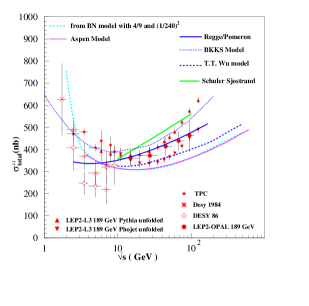
Figure 2: Predictions of models which treat photon like a proton

Here we have included the predictions of two QCD based models, the BN model 12 and the Aspen Model 13 , as well. We do see that the BN model does quite well with the fall at low energies as well. In Fig. 3 we compare the predictions of the EMM model in the total formulation for $\sigma_{\gamma p}$, with the data.

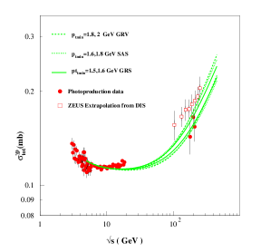
Figure 3: EMM predictions for $\sigma_{\gamma p}$ with different densities for the photonic partons 8 ; GRV ; GRS .

Note that the newer data on $\sigma^{tot}_{\gamma p}$ obtained by the extrapolation of the DIS data to photoproduction limit 2' lies consistently above the $\sigma^{tot}_{\gamma p}$ measured previously 2 . The A(b) here is modelled as the Fourier Transform of the product of electromagnetic form factors for the proton and the experimentally measured transverse momentum distribution for photonic partons. Here we have used the central value of the parameter $k_{0}$ = 0.66 where the transverse momentum distribution is measured 14 to be $\propto$ $1/(k_{T}^{2}+k_{0}^{2})$. Having fixed all the values by $\sigma^{\rm tot}_{\gamma p}$, if we now calculate $\sigma^{\rm tot}_{\gamma\gamma}$ we get predictions shown in Fig. 4.

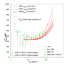
Figure 4: Comparison of the older LEP2 data with predictions of the EMM model in the total formulation for different photonic parton densities.

In this figure we have the $189$ GeV data from the OPAL 3 and L3 4 collaborations. Fig. 5 shows the $A_{\gamma\gamma}(b)$ 11 for different values of $k_{0}$, allowed by the experimental measurement 14 of $k_{0}=0.66\pm 0.22$.

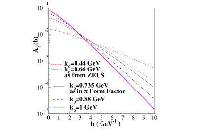
Figure 5: $A_{\gamma\gamma}$ for different values of $k_{0}$.

As $k_{0}$ decreases (increases), the curves in Fig. 4 will move up (down). Actually Fig. 6 shows the prediction of the EMM model using $k_{0}=0.4$ along

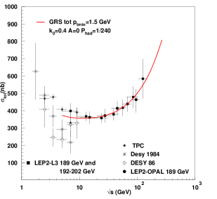
Figure 6: Latest LEP2 data along with EMM prediction in total formulation with $k_{0}$ = 0.4

with the same OPAL data as in Fig. 4 and the latest L3 data 15 . Values of all the other parameters which have been used are as given in the figure. We see that the EMM model is able to produce the trend of the faster rise quite well. Fig.  7 shows a comparison of all the model predictions with each other and the data. We notice that the rate of rise of total cross-sections in the EMM/BKKS models is quite different from those in Regge-Pomeron type models.

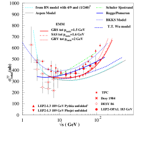
Figure 7: A comparison of all the various model predictions with the latest data.

Table 1: Predictions for different ‘proton-like’ models

$\sqrt{s_{\gamma\gamma}}(GeV)$	Aspen	T.T. Wu	DL	$1\sigma$
20	309 nb	330 nb	379 nb	7%
50	330 nb	368 nb	430 nb	11%
100	362 nb	401 nb	477 nb	10%
200	404 nb	441 nb	531 nb	9%
500	474 nb	515 nb	612 nb	8%
700	503 nb	543 nb	645 nb	8%

Table 2: Predictions for different QCD based models.

$\sqrt{s_{\gamma\gamma}}$	EMM,Inel,GRS	EMM,Tot,GRV	BKKS	$1\sigma$
	($p_{tmin}$=1.5 GeV)	($p_{tmin}$=2 GeV)	GRV
20	399 nb	331 nb	408 nb	2 %
50	429 nb	374 nb	471 nb	9%
100	486 nb	472 nb	543 nb	11%
200	596 nb	676 nb	635 nb	6%
500	850 nb	1165 nb	792 nb	7 %
700	978 nb	1407 nb	860 nb	13 %

The tables 1 and 2, give the precision with which $\sigma_{\gamma\gamma}$ needs to be measured, at the $\gamma\gamma$ colliders with $\sqrt{s_{\gamma\gamma}}$ in the range of 300-500 GeV, to be able to distinguish between the different ’photon is like a proton’ models as well as the EMM/BKKS models. As we can see, a precision of $\lessapprox 7\%$ is required to distinguish among the different ’photon like a proton’ models from one another, whereas only a precision of $\lessapprox 20\%$ is required to distinguish these predictions from those of the QCD based/inspired models which tend to predict a faster rise, in the energy range $300<\sqrt{s_{\gamma\gamma}}<500$ GeV. With $\gamma\gamma$ cm energy $\approx 700$ GeV, the difference between the predictions of the Aspen 13 and EMM total formulation 6 can be as large as a factor of 2.

However, when these $\gamma\gamma$ cross-sections are convoluted with the spectrum of the bremsstrahlung photons to calculate $\sigma$ ($e^{+}e^{-}\to e^{+}e^{-}{\gamma\gamma}\to e^{+}e^{-}X)$ using the WW approximation, we find that these big differences get reduced to about $30\%$. this is shown in Fig. 8. This demonstrates the much more superior role that the $\gamma\gamma$ colliders can play in deciding which is the right theoretical framework for calculation of total cross-sections .

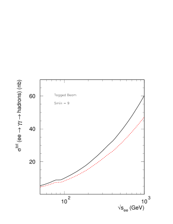
Figure 8: Total hadron production cross-section via two-photon processes at $e^{+}e^{-}$ colliders.

4 Conclusions

Thus in conclusion we can say the following

1. ’Photon is like a proton’ models predict a rise of $\sigma_{\gamma\gamma}$ with $\sqrt{s_{\gamma\gamma}}$, slower than shown by the data; i.e. value of predicted $\epsilon$ is lower than what the data seem to show.

2. The extrapolated $\gamma p$ data seem to show similar trends.

3. The predictions of the EMM model show good agreement with the data.

4. Even in the EMM formulations use of Bloch Nordsieck ideas to calculate the overlap function $A(b)$ seems to slow down this rise.

5. An obvious improvement in the EMM models is to try and determine $A(b)$ by more refined ‘theoretical’ ideas or determine it in terms of the multiple parton interactions measured at the HERA/Tevatron collider.

6. However, extraction of $\sigma_{\gamma\gamma}$ and $\sigma_{\gamma p}$ from $\sigma_{e^{+}e^{-}}$ and $\sigma_{ep}$ respectively, is no mean task and has large uncertainties. Moreover, a difference of about a factor two in the predicted values of $\sigma^{\rm tot}_{\gamma\gamma}$ in different models, gets reduced to only about $30\%$ when folded with the photon spectrum expected in the WW approximation in $e^{+}e^{-}$ collisions. While the good part is that it reduces the uncertainty in our predictions of the hadronic background at the $e^{+}e^{-}$ linear colliders due to the corresponding uncertainties in $\sigma^{\rm tot}_{\gamma\gamma}$, the studies of two-photon hadronic cross-sections at $e^{+}e^{-}$ colliders, will not be very efficient in shedding much light on the theortical models used to calculate them.

7. Therefore measurements of total cross-sections at a $\gamma\gamma$ collider with its monochromatic photon beam, in the energy range $300<\sqrt{s_{\gamma\gamma}}<500$ GeV, can play a very useful role in furthering our understanding of the ’high’ energy photon interactions. A precision of $\lessapprox 7-8\%(8-9\%)$ is required to distinguish among the different formulations of the EMM models (models which treat photon like a proton), where as a precision of $\lessapprox 20\%$ is required to distinguish betwen these two types of models.

5 Acknowledgements:

We grateful to A. de Roeck for the suggestion to study the issue of precision of measurement at the linear colliders.

References

- (1) M. Drees and R.M. Godbole, Phys. Rev. Lett. 67 (1991) 1189; P. Chen ,T. Barklow and M.E. Peskin, Phys. Rev. D49 (1994) 3209, R.M. Godbole, hep-ph/9807379, Proceedings of the Workshop onQuantum Aspects of Beam Physics, Jan. 5 1998 - Jan. 9 1998, Monterey, U.S.A., 404-416, Ed. P. Chen, World Scientific, 1999.
- (2) E. Accomando et al., Phys. Rep. 299 (1998) 1, hep-ph/9705442.
- (3) ZEUS Collaboration, Phys. Lett. B 293 (1992), 465; Zeit. Phys. C 63 (1994) 391; H1 Collaboration, Zeit. Phys. C69 (1995) 27.
- (4) J. Breitweg et al., ZEUS coll., DESY-00-071, e-print Archive: hep-ex/0005018.
- (5) OPAL Collaboration. F. Waeckerle, Multiparticle Dynamics 1997, Nucl. Phys. Proc. Suppl. B71, (1999) 381, Eds. G. Capon, V. Khoze, G. Pancheri and A. Sansoni; Stefan Söldner-Rembold, hep-ex/9810011, To appear in the proceedings of the ICHEP’98, Vancouver, July 1998. G. Abbiendi et al.,Eur.Phys.J.C14 (2000) 199.
- (6) L3 Collaboration, Paper 519 submitted to ICHEP’98, Vancouver, July 1998. M. Acciari et al., Phys. Lett. B 408 (1997) 450; L3 Collaboration, A. Csilling, Nucl.Phys.Proc.Suppl. B82 (2000) 239.
- (7) R.M. Godbole, A. Grau and G. Pancheri. Nucl.Phys.Proc.Suppl.B82 (2000), hep-ph/9908220.
- (8) L3 Collaboration, L3 Note 2548, Submitted to the International High Energy Physics Conference, Osaka, August 2000.
- (9) R.M. Godbole and G. Pancheri, In preparation.
- (10) A. Donnachie and P.V. Landshoff, Phys. Lett.B 296 (1992) 227.
- (11) G. Schuler and T. Sjöstrand, Zeit. Physik C 68 (1995) 607; Phys. Lett. B 376 (1996) 193.
- (12) C. Bourelly, J. Soffer and T.T. Wu, Mod.Phys.Lett. A15 (2000) 9.
- (13) B. Badelek, M. Krawczyk, J. Kwiecinski and A.M. Stasto. e-Print Archive: hep-ph/0001161.
- (14) A. Corsetti, R.M. Godbole and G. Pancheri, Phys.Lett. B435 (1998) 441.
- (15) A. Grau, G. Pancheri and Y.N. Srivastava, Phys.Rev. D60 (1999) 114020.
- (16) M.M. Block, E.M. Gregores, F. Halzen and G. Pancheri, Phys.Rev.D58 (1998) 17503; M.M. Block, E.M. Gregores, F. Halzen and G. Pancheri, Phys.Rev. D60 (1999) 54024.
- (17) M. Derrick et al., ZEUS coll., Phys. Lett. B 354 (1995) 163.
- (18) M. Glück, E. Reya and A. Vogt, Zeit. Physik C 67 (1994) 433 . M. Glück, E. Reya and A. Vogt, Phys. Rev. D 46 (1992) 1973.
- (19) M. Glück, E. Reya and I. Schienbein, Phys.Rev.D60:054019, 1999, Erratum-ibid.D62:019902,2000.