QCD Signatures of Narrow Graviton Resonances in Hadron Colliders

Abstract

We show that the characteristic $p_{\perp}$ spectrum yields valuable information for the test of models for the production of narrow graviton resonances in the TeV range at LHC. Furthermore, it is demonstrated that in those scenarios the parton showering formalism agrees with the prediction of NLO matrix element calculations.

I Introduction

The search for particles beyond the Standard Model is one of the key issues of the upcoming ATLAS and CMS experiments at LHC. If these particles are generated from quarks and gluons, characteristic signatures are expected from genuine QCD effects such as parton showering. As a specific example we study the narrow graviton resonances predicted by the Randall-Sundrum model [1]. As opposed to the concept of Large Extra Dimensions [2], where a continuous spectrum of Kaluza-Klein states is predicted, the Randall-Sundrum model predicts a series of narrow heavy graviton resonances. Both models lead to a modification of the gravitation potential at small distances $R$. While in case of two large extra dimensions the precision reachable at LHC ($R=4.5\;{\rm\mu}$m [3]) is roughly comparable to present mechanical experiments ($R=218\;{\rm\mu}$m [4]), signatures for the Randall-Sundrum type of gravitons can only be seen in TeV-scale collider experiments.

Recently, in the context of the Randall-Sundrum model the signatures of narrow graviton resonances at TeV-scale have been studied in Ref. [5]. Here the processes $gg\to G\to e^{+}e^{-}$ and $q\bar{q}\to G\to e^{+}e^{-}$ are of interest as their leptonic final states provide a clean and simple way to identify the heavy graviton resonance $G$. The main experimental signature for such a spin-2 graviton resonance is the characteristic angular distribution of the produced $e^{+}e^{-}$ pair. As the extraction of the angular distribution is quite difficult even with high luminosity, further characteristic signatures are desirable to make conclusive statements.

One possibility of such a complementary signature is the $p_{\perp}$ spectrum ($p_{\perp}$ is the transverse momentum with respect to the beam direction) of the reconstructed graviton resonance $G$. The production mechanism is given by a characteristic mixture of $gg$ and $q\bar{q}$ fusion processes. As those processes are highly energetic, the initial-state partons will radiate off a large amount of other partons, leading to a $p_{\perp}$ spectrum which is different for $gg$ and $q\bar{q}$ initial states. Especially, the larger color charge of the gluon will lead to more radiation and a larger average $p_{\perp}$ in the former process. So by studying the $p_{\perp}$ spectrum, one can check the ratio of $q\bar{q}$ and $gg$ events producing the resonance in question and compare that to the prediction of a certain model, in our case the Randall-Sundrum model.

II Physical Subprocesses

The partonic subprocesses of interest to discover the narrow graviton resonance $G$ are $gg\to G\to l^{+}l^{-}$ and $q\bar{q}\to G\to l^{+}l^{-}$, as depicted in Fig. 1 a,b. The relevant Standard Model background is the $l^{+}l^{-}$ pair production from virtual $Z^{0}$ bosons and photons, see Fig. 1 c,d, and their interference. The interference with the narrow graviton resonance can be completely neglected since the mass of the graviton, if existent, has to lie far above the $Z^{0}$ mass.

FIG. 1.: Signal and Standard Model background processes for the graviton resonance production.

For the cross sections (a) and (b) of the processes depicted in Fig. 1 we reproduce in accordance with Ref. [6, 7]:

$$\frac{d\sigma^{(a)}}{dt} = \frac{1}{N_{c}}\frac{\kappa^{4}s^{2}}{2048\pi}\frac{1+10x+42x^{2}+64x^{3}+32x^{4}}{(s-m_{G}^{2})^{2}+m_{G}^{2}\Gamma_{G}^{2}}$$ (1)

$$\frac{d\sigma^{(b)}}{dt} = \frac{\kappa^{4}s^{2}}{1024\pi}\frac{-x(1+x)(1+2x+2x^{2})}{(s-m_{G}^{2})^{2}+m_{G}^{2}\Gamma_{G}^{2}}\;.$$ (2)

Here we define as in Ref. [6] $x=t/s$. We set in accordance with Ref. [5] $\kappa=\sqrt{2}x_{1}k/({\bar{M}_{\rm Pl}}m_{G})$, where $k/{\bar{M}_{\rm Pl}}=0.01$ and $x_{1}=3.8317$ is the first zero of the Bessel function $J_{1}(x)$ of order 1. Higher zeros of the Bessel function $J_{1}(x)$ generate the series of heavy graviton resonances that the Randall-Sundrum model predicts. In the analysis here we will, however, restrict ourself to the first one. The total width $\Gamma_{G}$ of the spin-2 graviton $G$ with mass $m_{G}$ is determined by the sum of the following partial decay widths [5, 7]:

$$\Gamma(G\to V\bar{V}) = \delta\frac{\kappa^{2}m_{G}^{3}}{80\pi}(1-4r_{V})^{1/2}\left(\frac{13}{12}+\frac{14}{3}r_{V}+4r_{V}^{2}\right)$$ (4)

$$\Gamma(G\to f\bar{f}) = N_{c}\frac{\kappa^{2}m_{G}^{3}}{320\pi}(1-4r_{f})^{3/2}\left(1+\frac{8}{3}r_{f}\right)$$ (5)

$$\Gamma(G\to gg) = \frac{\kappa^{2}m_{G}^{3}}{20\pi}$$ (6)

$$\Gamma(G\to\gamma\gamma) = \frac{\kappa^{2}m_{G}^{3}}{160\pi}\;.$$ (7)

$V$ is a massive vector boson ($V=Z^{0},W^{\pm}$) with mass $m_{V}$ and $r_{V}=m_{V}^{2}/m_{G}^{2}$. For identical particles $\delta=1/2$ and for distinguishable particles $\delta=1$. $f$ is a fermion with mass $m_{f}$ and $N_{c}$ its number of colors, if there are any, otherwise $N_{c}=1$. Furthermore, we set $r_{f}=m_{f}^{2}/m_{G}^{2}$. In case of the width $\Gamma(G\to V\bar{V})$ we reproduce the result of Ref. [5], in all other cases the ones of Ref. [7].

III Event Generator Implementation

In order to study graviton production in a reasonably realistic framework, a single excited graviton $G$ has been introduced to the Pythia 6.1 event generator [8]. The $G$ mass and the dimensionless coupling parameter $\kappa m_{G}=\sqrt{2}x_{1}k/{\bar{M}_{\rm Pl}}$ can be set freely. Partial decay widths are given as above, and add up to a total width used for the resonance Breit-Wigner. The production processes $gg\to G$ and $q\bar{q}\to G$ are included, with relevant angular distribution for the subsequent decays of $G$ to a fermion pair (while other decays currently are isotropic only). The basic process is embedded in the standard Pythia framework of initial- and final-state QCD parton showers, underlying event activity (multiple interactions and beam remnants), fragmentation to hadrons and unstable particle decays. For $G$ decays to lepton pairs, the most notable effect may be the initial-state radiation of gluons off the incoming quarks and gluons, that gives a $p_{\perp}$ recoil to the produced $G$.

IV Simulation of the characteristic $p_{\perp}$ spectrum

We present as an example a simulation for the ATLAS experiment at LHC with $E_{\rm cm}=14$ TeV. In the following we have to investigate how well the hypothetical graviton mass can be reconstructed from the lepton pairs. A comprehensive study using the ATLFAST program [9] has been performed in Ref. [5] for $e^{+}e^{-}$ pairs. Here we want to add the experimental width for $\mu^{+}\mu^{-}$ pairs. For the graviton masses we use the same mass window as in Ref. [5], i.e 500 GeV $<m_{G}<$ 2200 GeV. As mentioned in Ref. [5] it will not be possible to detect gravitons with masses larger than about 2200 GeV at the ATLAS experiment in the scenario discussed here. On the other hand, already existing bounds limit the minimum graviton mass to $m_{G}>$ 500 GeV [10]. It should be noted that the choice for the coupling constant lies on the lower edge, in fact the allowed region favors rather $k/\bar{M}_{\rm Pl}=0.1$ than 0.01 [10] leading to a cross section which would be two order of magnitudes larger than the one we have assumed here, but then the graviton resonances would be no longer narrow. In this sense our estimates are conservative. As we are only interested in the principle effect we use here an approximative parameterization for the resolution of the ATLAS detector. For the electrons the following formula is used (see Ref. [11] pp. 114-115):

$$\left(\frac{\sigma(E)}{E}\right)^{2}_{\rm electrons}\approx\frac{(0.1)^{2}\;{\rm GeV}}{E}+(0.005)^{2}\;.$$ (8)

For the the muons, the combined ATLAS detector resolution for $p_{\perp}$ measurement, using both the muon spectrometer and the inner tracking detectors, is about $2\%$ below $p_{\perp}=100$ GeV, about $4\%$ at 300 GeV and about 7% at 1000 GeV (see Ref. [11] p. 242).

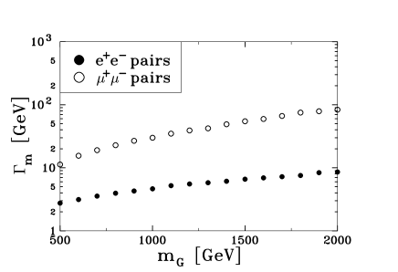
FIG. 2.: Graphical representation of the mass resolution $\Gamma_{m}$ of the ATLAS detector for narrow graviton resonances with mass $m_{G}$ reconstructed from $e^{+}e^{-}$ and $\mu^{+}\mu^{-}$ pairs for the ATLAS detector.

Furthermore, in order to have realistic trigger conditions, we take $e^{+}e^{-}$ pairs into account only if both of them have a pseudorapidity $|\eta|<2.5$. Both of them must in addition have a transverse energy larger than 20 GeV, or one of the two electrons has to have an $E_{\perp}$ of at least 30 GeV (see Ref. [11] p. 392). For the muon pairs we adopt corresponding conditions: both of them must have a pseudorapidity $|\eta|<2.4$, and both must have a transverse momentum $p_{\perp}$ larger than 6 GeV or one of them must have a $p_{\perp}$ of at least 20 GeV (see Ref. [11] p. 392). The number of muon-pair events is thus originally larger than the number of electron-pair events. The limited detector resolution leads to a smearing of the reconstructed graviton mass which can be fitted by a Gaussian distribution. The width of this Gaussian distribution defines the experimental width $\Gamma_{m}$. Fig. 2 shows the experimental graviton-mass resolution $\Gamma_{m}$ reconstructed from $e^{+}e^{-}$ and $\mu^{+}\mu^{-}$ pairs using the parameterizations given above. The values presented here for the $e^{+}e^{-}$ pairs agree roughly with the ones shown in Ref. [5] using the ATLFAST routine.

FIG. 3.: $p_{\perp}$ spectrum for $m_{G}=500$ GeV (top) and $m_{G}=2000$ GeV (bottom). In the figure is shown the Standard Model background from $\gamma,Z^{0}$ production (dashed-dotted) line, the $gg$ contribution (dashed line) and the $q\bar{q}$ contribution (solid line).

It has to be stated that in all cases the experimental width exceeds by far the physical width given by the lifetime of the graviton resonance [5]. But this is inessential for the forthcoming simulations as the results depend only weakly on the precise value of the experimental width and, furthermore, in this paper we only intend to show the principal effect. As a result, it is seen that the resolution for the electrons is nearly an order of magnitude better than for the muons, therefore, in the following we will concentrate ourselves on the electrons only. Only in cases where the statistical error will overwhelm the experimental resolution the muons might provide additional evidence. As a next step we simulate the $p_{\perp}$ spectrum for the two hypothetical graviton masses $m_{G}=500$ GeV and $m_{G}=2000$ GeV. For the simulations we use the width from Fig. 2. The $p_{\perp}$ distribution is created from initial-state parton showering only. The final-state parton shower complicates the situation only through photon bremsstrahlung. We have checked that these latter effects are small.

Fig. 3 shows the $p_{\perp}$ spectrum for $m_{G}=500\;{\rm GeV}$ (top) and $m_{G}=2000\;{\rm GeV}$ (bottom) split in the contributions $gg\to G\to e^{+}e^{-}$, $q\bar{q}\to G\to e^{+}e^{-}$ and the Standard Model background $q\bar{q}\to Z/\gamma\to e^{+}e^{-}$. To reduce the Standard Model background a window of $3\times\Gamma_{m}$ around the resonance maximum is taken. It is seen that for smaller resonance masses the contribution from gg fusion becomes dominant, but in both cases the maximum of the $p_{\perp}$ spectrum for the processes with a $q\bar{q}$ initial state (including the SM background) lies at considerable smaller values than the one for the gg-fusion process. Therefore, the characteristic shape of the $p_{\perp}$ spectrum allows to draw conclusions about the ratio of $q\bar{q}$ versus $gg$-processes and provides a cross check whether the underlying theoretical model is correct.

FIG. 4.: Average $p_{\perp}$, i.e. $\sqrt{\langle p_{\perp}^{2}\rangle}$, versus the graviton mass $m_{G}$. The open circles show the average $p_{\perp}$ for the $q\bar{q}\to G$ process, the full circles for the the $gg\to G$ process, and the open squares for the Standard Model background $q\bar{q}\to Z/\gamma$. The triangles show the total average $p_{\perp}$ for all processes including the Standard Model background, with error bars for a luminosity of ${\cal L}=100\;{\rm fb}^{-1}$.

To quantify this we regard in Fig. 4 the average $p_{\perp}$, i.e. $\sqrt{\langle p_{\perp}^{2}\rangle}$. The triangles show the total average $p_{\perp}$, where all processes including the SM background contribute. For the errors we use the parameterization in Eq. 8 for the electrons plus a statistical error given by the root of the number of events. For the simulation we assume a luminosity of ${\cal L}=100\;{\rm fb}^{-1}$. This is the high luminosity planned for the ATLAS detector [11]. One sees that even for the highest mass values for the graviton mass, i.e. $m_{G}=2200\;{\rm GeV}$ the pure $q\bar{q}$ fusion hypothesis lies outside the 1 $\sigma$ range of the combined $q\bar{q}$ and $gg$ fusion hypothesis. Furthermore, one observes that for values smaller than $m_{G}=1200\;{\rm GeV}$ the gg fusion is so dominant that the total average $p_{\perp}$ nearly coincides with the one of gg fusion only. The average $p_{\perp}$ of the Standard Model background alone lies a bit above the $q\bar{q}\to G$ processes. The difference between the two $q\bar{q}$-induced processes mainly comes from the $q\bar{q}\to Z/\gamma$ parton shower being matched to first order matrix elements at large $p_{\perp}$ [8]. A careful study of the $p_{\perp}$ spectrum as a whole will be very helpful to distinguish possible Randall-Sundrum graviton resonances from pure $q\bar{q}$ based exotic resonances like a $Z^{\prime}$.

The characteristic features of the $p_{\perp}$ spectrum may also be at help to enhance the angular distribution of the $gg\to G\to e^{+}e^{-}$ channel relative to the $q\bar{q}\to G\to e^{+}e^{-}$ channel by cutting out $e^{+}e^{-}$ pairs with low $p_{\perp}$. The full information content is available in the doubly differential distribution of $p_{\perp}$ and $e^{+}e^{-}$ decay angle together (Eq. LABEL:angle). A complete analysis of this issue, e.g. using a likelihood analysis is, however, beyond the scope of this article.

V Matrix elements versus showering formalism

The $p_{\perp}$ spectrum described in the previous chapter has been generated by the parton showering formalism. As this is only an approximation, it is important to check how well it models the description by a full matrix element calculation. For this purpose we consider the next to leading order graviton production matrix elements.

FIG. 5.: NLO amplitudes for the resonance production of gravitons $G$, with the subprocesses $gg\to Gg$ (top) and $q\bar{q}\to Gg$ (bottom).

Fig. 5 shows the NLO contributions to graviton production for the processes $g(k_{1})+g(k_{2})\to g(k_{j})+G$ and $q(k_{1})+\bar{q}(k_{2})\to g(k_{j})+G$. For the Mandelstam variables we define $s=(k_{1}+k_{2})^{2}$, $t=(k_{1}-k_{j})^{2}$, and $u=(k_{2}-k_{j})^{2}$, see Fig. 6, where $k_{j}$ denotes the momentum of the outgoing parton jet. Then we have the relation $m_{G}^{2}=s+t+u$. In the following we use the shorthand notation $k=k_{1}+k_{2}$. The gluon polarization tensor is noted by $\epsilon^{A\rho}(k_{j})$ and the graviton polarization tensor by $\epsilon^{\mu\nu}(k_{gr})$, where $k_{gr}=k-k_{j}$ is the graviton’s four-momentum. For the processes $q\bar{q}\to Gg$ the amplitude reads:

$$M_{q\bar{q}\to Gg}=\frac{i}{2}g\kappa\bar{v}(k_{2})t^{A}\Bigg{[}\frac{1}{t}\gamma_{\mu}(\parbox[b]{6.00006pt}{$k$}\parbox[b]{5.50003pt}{ \raisebox{-0.86108pt}{$/$}}_{1}-\parbox[b]{6.00006pt}{$k$}\parbox[b]{5.50003pt}{ \raisebox{-0.86108pt}{$/$}}_{j})\gamma_{\rho}k_{2\nu}$$ (9)

$$\qquad+\frac{1}{u}\gamma_{\rho}(\parbox[b]{6.00006pt}{$k$}\parbox[b]{5.50003pt}{ \raisebox{-0.86108pt}{$/$}}_{2}-\parbox[b]{6.00006pt}{$k$}\parbox[b]{5.50003pt}{ \raisebox{-0.86108pt}{$/$}}_{j})\gamma_{\mu}k_{1\nu}-\frac{2}{s}\gamma^{\sigma}\Bigg{(}k\cdot k_{j}g_{\mu\rho}g_{\nu\sigma}$$ (10)

$$\qquad+g_{\rho\sigma}k_{j\mu}k_{\nu}-g_{\mu\sigma}k_{j\nu}k_{\rho}-g_{\mu\rho}k_{j\sigma}k_{\nu}\Bigg{)}$$ (11)

$$\quad+g_{\mu\rho}\gamma_{\nu}\Bigg{]}u(k_{1})\epsilon^{A\rho}(k_{j})\epsilon^{\mu\nu}(k_{gr})\;.$$ (12)

Here we reproduce the results of Ref. [7]. For the differential cross section we obtain in agreement with Ref. [6]:

$$\frac{d\sigma_{q\bar{q}\to Gg}}{dt} = \frac{\alpha_{s}\kappa^{2}}{64s}\frac{N_{c}^{2}-1}{N_{c}^{2}}\Bigg{[}4\frac{t^{2}+u^{2}}{s^{2}}+9\frac{t+u}{s}$$ (15)

$$+\frac{1}{s}\left(\frac{t^{2}}{u}+\frac{u^{2}}{t}\right)+3\left(4+\frac{t}{u}+\frac{u}{t}\right)$$

$$+4s\left(\frac{1}{u}+\frac{1}{t}\right)+\frac{2s^{2}}{tu}\Bigg{]}$$

$$= \frac{\alpha_{s}\kappa^{2}}{64s^{2}}\frac{N_{c}^{2}-1}{N_{c}^{2}}F(s,t,u)$$ (16)

The cross sections for the processes $qg\to qG$ and $\bar{q}g\to\bar{q}G$ can be obtained from this by a simple rotation of the Mandelstam variables:

$$\frac{d\sigma_{qg\to Gq}}{dt}=\frac{d\sigma_{\bar{q}g\to G\bar{q}}}{dt}=\frac{\alpha_{s}\kappa^{2}}{64s^{2}N_{c}}F(t,s,u)\;.$$ (17)

FIG. 6.: Definition of the Mandelstam variables for the processes $q\bar{q}\to gG$ (left) and $qg\to qG$, $\bar{q}g\to\bar{q}G$ (right).

For the amplitude of the process $gg\to Gg$ one gets using gauge invariance (where the gauge dependent terms of the inner gluon propagator vanish identically):

$$M_{gg\to Gg}=\frac{\kappa g}{2}f^{ABC}\Bigg{\{}\frac{1}{t}G_{\alpha\beta}^{\quad\sigma}(k_{j},-k_{1},k_{1}-k_{j})$$ (18)

$$\quad\quad\times[k_{2}\cdot(k_{1}-k_{j})C_{\mu\nu,\rho\sigma}+D_{\mu\nu,\rho\sigma}(k_{2},k_{1}-k_{j})]$$ (19)

$$\;\;+\frac{1}{u}G_{\rho\alpha}^{\quad\sigma}(-k_{2},k_{j},k_{2}-k_{j})$$ (20)

$$\quad\quad\times[k_{1}\cdot(k_{2}-k_{j})C_{\mu\nu,\beta\sigma}+D_{\mu\nu,\beta\sigma}(k_{1},k_{2}-k_{j})]$$ (21)

$$\;\;+\frac{1}{s}G_{\beta\rho}^{\quad\sigma}(-k_{1},-k_{2},k_{1}+k_{2})$$ (22)

$$\quad\quad\times[-k_{j}\cdot(k_{1}+k_{2})C_{\mu\nu,\alpha\sigma}+D_{\mu\nu,\alpha\sigma}(-k_{j},k_{1}+k_{2})]$$ (23)

$$\;\;+[C_{\mu\nu,\rho\beta}(k_{2}-k_{1})_{\alpha}+C_{\mu\nu,\rho\alpha}(-k_{j}-k_{2})_{\beta}$$ (24)

$$\;\;\;+C_{\mu\nu,\beta\alpha}(k_{1}+k_{j})_{\rho}+F_{\mu\nu,\rho\beta\alpha}(k_{2},k_{1},-k_{j})]\Bigg{\}}$$ (25)

$$\times\epsilon^{\alpha A}(k_{j})\epsilon^{\beta B}(k_{1})\epsilon^{\rho C}(k_{2})\epsilon^{\mu\nu}(k_{gr})\;.$$ (26)

Here the following definitions are used:

$$C_{\mu\nu,\rho\sigma} = 2g_{\mu\sigma}g_{\nu\rho}$$ (27)

$$D_{\mu\nu,\rho\sigma}(k_{1},k_{2}) = -2(g_{\mu\sigma}k_{1\nu}k_{2\rho}+g_{\mu\rho}k_{1\sigma}k_{2\nu}$$ (29)

$$\quad-g_{\rho\sigma}k_{1\mu}k_{2\nu})$$

$$F_{\mu\nu,\rho\sigma\lambda}(k_{1},k_{2},k_{3}) = 2(g_{\mu\lambda}g_{\rho\sigma}(k_{1}-k_{2})_{\nu}$$ (32)

$$\quad+g_{\mu\rho}g_{\sigma\lambda}(k_{2}-k_{3})_{\nu}$$

$$\quad+g_{\mu\sigma}g_{\lambda\rho}(k_{3}-k_{1})_{\nu})$$

$$G_{\rho\sigma\lambda}(k_{1},k_{2},k_{3}) = g_{\rho\sigma}(k_{1}-k_{2})_{\lambda}+g_{\sigma\lambda}(k_{2}-k_{3})_{\rho}$$ (34)

$$+g_{\lambda\rho}(k_{3}-k_{1})_{\sigma}\;.$$

Furthermore, for the spin-sums over the polarization tensors one gets:

$$\sum_{s=1}^{5}\epsilon_{\mu\nu}^{s}(k_{g})\epsilon_{\rho\sigma}^{*s}(k_{g}) = \tilde{\eta}_{\mu\rho}\tilde{\eta}_{\nu\sigma}+\tilde{\eta}_{\mu\sigma}\tilde{\eta}_{\nu\rho}-\frac{2}{3}\tilde{\eta}_{\mu\nu}\tilde{\eta}_{\rho\sigma}$$ (35)

$$\tilde{\eta}_{\mu\nu} = g_{\mu\nu}-\frac{k_{g\mu}k_{g\mu}}{m_{G}^{2}}$$ (36)

$$\sum_{s=1}^{3}\epsilon_{\mu}^{sA}(k_{i})\epsilon_{\nu}^{*sB}(k_{i}) = \delta^{AB}\left(-g_{\mu\nu}+\frac{k_{i\mu}n_{i\nu}+k_{i\nu}n_{i\mu}}{k_{i}\cdot n_{i}}\right)$$ (37)

$$n_{i}\cdot n_{i} = 0;\quad(i=1,2,j)\;.$$ (38)

For the partonic cross section for the process $gg\to Gg$ we obtain then in agreement with Ref. [6]:

$$\frac{d\sigma_{gg\to Gg}}{dt} = \frac{N_{c}\kappa^{2}\alpha_{s}}{4s^{2}(N_{c}^{2}-1)}\Bigg{[}-4(s+t+u)$$ (40)

$$+\frac{(s^{2}+t^{2}+u^{2}+st+su+tu)^{2}}{stu}\Bigg{]}\;,$$

which shows the symmetry under the exchange of all three gluons with each other. These cross sections are implemented into the event generator Pythia 6.1 as well. Next we consider the ratio of the NLO matrix elements versus the LO matrix elements plus parton showering. For $p_{\perp}$ values larger than $100\;{\rm GeV}$ where soft effects and NNLO contributions are negligible this ratio should actually become equal to one in a certain range. Below $100\;{\rm GeV}$ a resummation procedure would have to be applied to tame the $p_{\perp}\to 0$ divergence of the NLO matrix elements, as is already implicit in the shower formalism. The situation is slightly complicated by the fact that the basic subprocesses that initiate the parton showering processes are only $q\bar{q}\to G$ and $gg\to G$, see Fig. 1, whereas the NLO matrix elements contain processes with $qg$ and $\bar{q}g$ initial parton states as well.

FIG. 7.: Assignment of $qg\to qG$ ($\bar{q}g\to\bar{q}G$) processes in the parton shower formalism. The figure shows a $qg\to qG$ process containing a $q\bar{q}\to G$ vertex (a) and a $gg\to G$ vertex (b).

The shower branchings effectively induce such initial states, see Fig. 7, so there is no fundamental conflict, but more a practical issue of comparing different classification schemes. In general, one would have to share the $qg/\bar{q}g$ NLO contributions between the $q\bar{q}$ and the $gg$ shower processes.

FIG. 8.: Comparison of matrix elements versus parton showering for the $q\bar{q}$ graviton production. Displayed is ratio of the NLO $q\bar{q}\to Gg$ cross section versus the LO cross section $q\bar{q}\to G$ plus parton showering.

We note however, that a $qg\to qG$ graph with a $gg\to G$ vertex (Fig. 7b) would receive contributions from t-channel gluon exchange, while the same graph with a $q\bar{q}\to G$ vertex (Fig. 7a) would instead contain u-channel quark exchange. The fact that the $qg\to qG$ cross section is strongly peaked at small $t$, and not at small $u$, indicates that $qg\to qG$ predominantly contributes to the $gg\to G$ graph and only little to $q\bar{q}\to G$. Fig. 8 shows the ratio $\sigma(q\bar{q}\to Gg)/\sigma(q\bar{q}\to G+PS)$ versus $p_{\perp}$. It is seen that for $p_{\perp}$ lower than $400$ GeV we find a good agreement between NLO matrix elements and the LO+parton shower, as the ratio here is nearly equal to one, as predicted by the reasoning above.

FIG. 9.: Comparison of matrix elements versus parton showering for graviton production involving gluons. Displayed is the ratio $\sigma(gg\to Gg)/\sigma(gg\to G+PS)$ (top) and $(\sigma(gg\to Gg)+\sigma(gq\to Gq)+\sigma(g\bar{q}\to G\bar{q}))/\sigma(gg\to G+PS)$ (bottom).

Fig. 9 shows that it is also reasonable to assign the $qg/\bar{q}g$ mixed initial states to the $gg\to G$ plus shower processes: If we only consider the ratio $\sigma(gg\to Gg)/\sigma(ggG+PS)$ one sees that in the range 100 GeV $<p_{\perp}<$ 400 GeV the matrix elements account for only 50% of the whole cross section coming from parton showering at some values of $p_{\perp}$. If one adds the quark-gluon matrix elements, however, the ratio is nearly equal to one up to 600 GeV. Therefore we find that the parton showering formalism is in good agreement with the cross section given by NLO matrix elements in the $p_{\perp}$ range between 100 GeV and 400 GeV. Below 100 GeV the shower formalism should give a trustworthy $p_{\perp}$ spectrum. Then the range we need for the analysis of the narrow graviton resonances is covered, see Fig. 4.

VI Summary

The $p_{\perp}$ spectrum is a supportive signature for the detection of narrow graviton resonances at LHC. It gives additional hints on the underlying production processes and may help to verify or to exclude certain scenarios such as the Randall-Sundrum model, because it is sensitive to a characteristic mixture of $gg$ and $q\bar{q}$ processes in graviton production unique for the corresponding model. Furthermore, we have shown that the parton showering formalism at TeV collider energies still gives a correct approximation of the predictions of matrix element calculations, so that the approximations in the parton showering formalism are justified also in this kind of processes yet experimentally untested.

REFERENCES

[1]
L. Randall and R. Sundrum,
Phys. Rev. Lett. 83, 3370 (1999)
[hep-ph/9905221].
[2]
N. Arkani-Hamed, S. Dimopoulos and G. Dvali,
Phys. Lett. B429, 263 (1998)
[hep-ph/9803315].
[3]
I. Antoniadis and K. Benakli,
hep-ph/0007226.
[4]
C. D. Hoyle, U. Schmidt, B. R. Heckel, E. G. Adelberger, J. H. Gundlach, D. J. Kapner and H. E. Swanson,
hep-ph/0011014.
[5]
B. C. Allanach, K. Odagiri, M. A. Parker and B. R. Webber,
JHEP 0009, 019 (2000)
[hep-ph/0006114].
[6]
G. F. Giudice, R. Rattazzi and J. D. Wells,
Nucl. Phys. B544, 3 (1999)
[hep-ph/9811291].
[7]
T. Han, J. D. Lykken and R. Zhang,
Phys. Rev. D59, 105006 (1999)
[hep-ph/9811350].
[8]
T. Sjöstrand, P. Edén, C. Friberg, L. Lönnblad, G. Miu,
S. Mrenna and E. Norrbin , LU TP 00–30 [hep-ph/0010017], to
appear in Computer Phys. Commun.
[9] E. Richter-Was, D. Froidevaux and L. Poggioli, “ATLFAST
1.0 A package for particle-level analysis”, ATLAS Internal Notes
ATL-PHYS-96-079 (1996) and ATL-PHY-98-131 (1998)
[10]
H. Davoudiasl, J. L. Hewett and T. G. Rizzo,
hep-ph/0006041.