Thermodynamics of the 3-flavor NJL model : chiral symmetry breaking and color superconductivity

F. Gastineau 1,R. Nebauer 1,2 and J.Aichelin 1
Abstract

Employing an extended three flavor version of the NJL model we discuss in detail the phase diagram of quark matter. The presence of quark as well as of diquark condensates gives rise to a rich structure of the phase diagram. We study in detail the chiral phase transition and the color superconductivity as well as color flavor locking as a function of the temperature and chemical potentials of the system.

1 SUBATECH, Laboratoire EMN, IN2P3-CNRS et Universit de Nantes,
F-44072 Nantes Cedex 03, France
2Institute for Theoretical Physics Universit t Rostock, Rostock, Germany

Introduction

At low temperatures and densities all quarks are confined into hadrons. In this phase the chiral symmetry is spontaneously broken by the quark condensates. Raising the temperature, one expects that the chiral symmetry becomes restored and the quarks are free. This state is called quark gluon plasma (QGP). In the QGP all symmetries of the QCD Lagrangian are restored. For QCD at low temperatures and high densities one expects a phase where the quarks are in a superconducting state [1, 2, 3, 4]. All this different phases define the phase diagram of QCD [5] in the plane of temperature and density. This phase diagram is not directly accessible. QCD calculations are only possible on a lattice at zero baryon density. In order to explore the finite temperature and density region, one has to rely on effective models. Two types of such effective models has been advanced to study the high density low temperature section The first type of models includes weak coupling QCD calculations, including the gluon propagators [6]. The second type include instanton [4, 7, 8] as well as Nambu and Jona-Lasinio (NJL) models [2, 9]. These models shows a color superconducting phase at high density and low temperature. In this phase the $SU_{C}(3)$ color symmetry of QCD breaks down to an $SU_{C}(2)$. Including a third flavor, another phase occurs, the color-flavor-locked state (CFL) of quark matter [9][11][12].

The two flavor results of the instanton approach are reproduced by the model of Nambu and Jona-Lasinio (NJL) [13][14] if one includes an appropriate interaction as was shown by Schwarz et al. [15]. This model has been extended by Langfeld and Rho [16] who included all possible interaction channels and discovered an even richer phase structure of the QCD phase diagram, including a phase where Lorentz symmetry is spontaneously broken.

The choice of the NJL model is motivated by the fact that this model displays the same symmetries as QCD and that it describes correctly the spontaneous breakdown of chiral symmetry in the vacuum and its restoration at high temperature and density. In addition, the NJL model has been successfully used to describe the meson spectra and thus is able to reproduce the low temperature and low density phenomena of QCD [17][18][19]. Thus, this is a model which starts out from the opposite direction as the instanton model which is motivated as high density approximation of QCD. Therefore it is interesting to see whether the NJL model is able to describe the other phases, the color superconducting phase and the color flavor locking observed in the instanton approach. The shortcoming of the NJL model is the fact that it does not describe confinement, or more generally any gauge dynamics at all. Here we will evaluate the thermodynamical properties of the quarks in the NJL model at finite temperature and density and we will discuss the symmetries of the different phases. We present numerical results for the calculation of the different condensates. For our study of the phase diagram we use one specific set of parameters.We treat the three flavor version of the model, including an interaction in the quark-antiquark channel, a tโ€™Hooft interaction and an interaction in the diquark channel. We restrict ourself to the scalar/ pseudoscalar sector of these interactions.

The paper is organized as follows: In chapter 1 we will briefly review the NJL model and present the Lagrangian we will use. In chapter 2 we study the quark condensate and the restoration of chiral symmetry. In chapter 3 we add the interaction in the diquark channel and present the numerical results for the color superconducting sector. We will have a complete evaluation of the phase diagram of the NJL model, including chiral and superconducting phase transition at finite temperature and (strange and light quark) density. In chapter 4 we present our conclusions.

1 The model

The model we use is an extended version of the NJL model, including an interaction in the diquark channel. In fact, the NJL model can be shown to be the simplest low energy approximation of QCD. It describes the interaction between two quark currents as a point-like exchange of a perturbative gluon [20][21]. Applying an appropriate Fierz-transformation to this interaction, the Lagrangian separates into two pieces: a color singlet interaction between a quark and an antiquark ($\mathscr{L}_{(\bar{q}q)}$) and a color antitriplet interaction between two quarks $\mathscr{L}_{(qq)}$. The color singlet channel is attractive in the scalar and pseudoscalar sector and repulsive in the vector and pseudovector channel. The Lagrangian in the diquark sector has two parts, both attractive: a flavor antisymmetric and flavor symmetric channel. The former includes Lorentz scalar, pseudoscalar and vector interactions, the latter a pseudo scalar interaction only.

The coupling constants of these different channels are related to each other by the Fierz transformation. Due to the extreme simplification of the gluon propagator in this approximation, the resulting model cannot reproduce confinement which is described by the infrared behavior of the gluon propagator.

The resulting Lagrangian has a global axial symmetry $U_{A}(1)$, and an extra term $\mathscr{L}_{A}$ in the form of the tโ€™Hooft determinant is added in order to break explicitly this symmetry. The resulting Lagrangian has then the general form:

$$\mathscr{L}=\mathscr{L}_{0}+\mathscr{L}_{(\bar{q}q)}+\mathscr{L}_{(qq)}+\mathscr{L}_{A}$$ (1)

where $\mathscr{L}_{0}$ is the free kinetic part.

The interaction part of the Lagrangian has a global color, flavor and chiral symmetry. Chiral symmetry is explicitly broken by non zero current quark masses, flavor symmetry by a mass difference between the flavors.

The different interaction channels of this Lagrangian give rise to a very rich structure of the phase diagram, which was completely evaluated in the two flavor case by Langfeld and Rho [16]. Here we will concentrate on the three flavor case. The evaluation of the complete phase structure in the three flavor case is a quite difficult task and we will concentrate here on the Lorentz scalar and pseudoscalar interactions. In the mesonic channel this interaction is responsible for the appearance of a quark condensate and for the spontaneous breakdown of the chiral symmetry. In the diquark channel it gives rise to a diquark condensate which can be identified with a superconducting gap.

Describing the quark fields by the Dirac-spinors $q$, the Lagrangian we will use here has the form:

$\displaystyle\mathscr{L}$ $\displaystyle=$ $\displaystyle\bar{q}(i{\partial}\!\!\!{/}-m_{0f})q+G_{S}\sum^{8}_{a=0}\left[(\bar{q}\lambda_{F}^{a}q)^{2}+(\bar{q}i\gamma_{5}\lambda_{F}^{a}q)^{2}\right]$
$\displaystyle+G_{DIQ}\sum^{3}_{k=1}\sum^{3}_{\gamma=1}\left[(\bar{q}_{i,\alpha}\epsilon^{ijk}\epsilon^{\alpha\beta\gamma}q_{j,\beta}^{C})(\bar{q}_{i^{\prime},\alpha^{\prime}}^{C}\epsilon^{i^{\prime}j^{\prime}k}\epsilon^{\alpha^{\prime}\beta^{\prime}\gamma}q_{j^{\prime},\beta^{\prime}})\right]$
$\displaystyle+G_{DIQ}\sum^{3}_{k=1}\sum^{3}_{\gamma=1}\left[(\bar{q}_{i,\alpha}i\gamma_{5}\epsilon^{ijk}\epsilon^{\alpha\beta\gamma}q_{j,\beta}^{C})(\bar{q}_{i^{\prime},\alpha}^{C}i\gamma_{5}\epsilon^{i^{\prime}j^{\prime}k}\epsilon^{\alpha^{\prime}\beta^{\prime}\gamma}q_{j^{\prime},\beta^{\prime}})\right]$
$\displaystyle+G_{D}\left[det\bar{q}(1-i\gamma_{5})q+det\bar{q}(1+i\gamma_{5})q\right].$

The first term is the free kinetic part, including the flavor dependent current quark masses $m_{0f}$ which break explicitly the chiral symmetry of the Lagrangian. The second part is the scalar/ pseudoscalar interaction in the mesonic channel, it is diagonal in color. The matrices $\lambda_{F}$ act in the flavor space. The third part describes the interaction in the scalar/ pseudoscalar diquark channel. The charge conjugated quark fields are denoted by $q^{C}=C\bar{q}^{T}$ and the color ($\alpha,\beta,\gamma$) and flavor ($i,j,k$) indices are displayed explicitly. We note that due to the charge conjugation operation the product $\bar{q}i\gamma_{5}q^{C}$ is a Lorentz scalar. This interaction is antisymmetric in flavor and color, expressed by the completely antisymmetric tensor $\epsilon^{ijk}$. Finally we add the six point interaction in the form of the tโ€™Hooft determinant which breaks explicitly the $U_{A}(1)$ symmetry of the Lagrangian. The $det$ runs over the flavor degrees of freedom, consequently the flavors become connected.

The NJL model is non renormalizable, thus it is not defined until a regularization procedure has been specified. As we are interested in the thermodynamical properties of the model, calculated with help of the thermodynamical potential, we will use a three dimensional cut-off in momentum space. This cut-off limits the validity of the model to momenta well below the cut-off.

The model contains six parameters: The current mass of the light and strange quarks, the coupling constants $G_{D}$ and $G_{S}$ and the momentum cut-off $\Lambda$ which are fixed by physical observables: the pion and kaon mass, the pion decay constant, the mass difference between $\eta$ and $\eta^{\prime}$ , once the mass of the light quarks was fixed, as well as by the vacuum value of the condensate $<q\bar{q}>^{1/3}=-230MeV$. The last parameter is the coupling constant in the diquark channel $G_{DIQ}$. For the mesonic sector we will use the parameters of [22]: a current light quark mass $m_{0q}=5.5\,MeV$, a current strange quark mass m0โ€‹s=140.7โ€‹Mโ€‹eโ€‹Vsubscript๐‘š0๐‘ 140.7๐‘€๐‘’๐‘‰m_{0s}=140.7\,MeV, a three dimensional ultraviolet cut-off $\Lambda=620\,MeV$, a scalar coupling constant $G_{S}=1.835/\Lambda^{2}$ and a determinant coupling $G_{D}=12.36/\Lambda^{5}$.. This parameter set results in effective vacuum quark masses of $m_{q}=367.6\,MeV$ , ms=549.5โ€‹Mโ€‹eโ€‹Vsubscript๐‘š๐‘ 549.5๐‘€๐‘’๐‘‰m_{s}=549.5\,MeV and the quark condensates are $\langle\!\langle\bar{q}q\rangle\!\rangle=(-242\,MeV)^{-3}$ and โŸจโŸจsยฏโ€‹sโŸฉโŸฉ=(โˆ’258โ€‹Mโ€‹eโ€‹V)โˆ’3delimited-โŸจโŸฉdelimited-โŸจโŸฉยฏ๐‘ ๐‘ superscript258๐‘€๐‘’๐‘‰3\langle\!\langle\bar{s}s\rangle\!\rangle=(-258\,MeV)^{-3}.

We perform our calculations in the mean field approach for an operator product

$$\hat{\rho}_{1}\hat{\rho}_{2}\approx\hat{\rho}_{1}\langle\!\langle\rho_{2}\rangle\!\rangle+\langle\!\langle\rho_{1}\rangle\!\rangle\hat{\rho}_{2}-\langle\!\langle\rho_{1}\rangle\!\rangle\langle\!\langle\rho_{2}\rangle\!\rangle$$ (3)

where $\langle\!\langle\rho\rangle\!\rangle$ is the thermodynamical average of the operator and the fluctuations around this mean value are supposed to be small. We will apply this approximation to the products of quark fields appearing in the interaction part of the Lagrangian.

2 Chiral phase transition

We start our study with an investigation of the quark-antiquark sector and the chiral phase transition. The diquark sector is subject of the next section.

The NJL model displays the right features of the chiral symmetry breaking. On the one hand we have an explicitly broken chiral symmetry by the inclusion of a small current quark mass. On the other hand, the model describes correctly the spontaneous breakdown of chiral symmetry: the existence of a quark condensate, responsible for a high effective quark mass and the existence of massless (or very light, if the chiral symmetry is explicitly broken) Nambu-Goldstone bosons. Lattice QCD calculations show that at a temperature of $\approx 170MeV$ the chiral symmetry is restored (the quark condensates melt at increasing temperature), a result which is reproduced by the NJL model [17][18][10]. As the region of finite density is not accessible to lattice QCD calculations, the chiral phase transition at high density is a subject of speculation. The point and the order of the chiral phase transition in the temperature - density plane defines the phase diagram. Here we will present such a phase diagram for the three flavor NJL model and a specified set of parameters. This phase diagram can be viewed as an approximation of the QCD phase diagram, but we have to take into account that the NJL model does not describe confinement (we always have a gas of quarks and not a gas of hadrons) and that the degrees of freedom are not the same as in QCD (the model contains no gluons). Here we will focus on the thermodynamical properties of the quarks described in the color singlet channel of the Lagrangian (1), this means the thermodynamical properties of the quark condensates and masses.

For the study of the thermodynamical properties of the quark-antiquark sector we will evaluate the thermodynamical potential in the mean field approximation. We start out from the Lagrangian in the mean field approximation

$$\mathscr{L}^{MF}=\bar{q}(i{\partial}\!\!\!{/}-M)q-2G_{S}(\alpha^{2}+\beta^{2}+\gamma^{2})+4G_{D}\alpha\beta\gamma.$$ (4)

where $M_{f}$ is the effective quark mass (defined via the quark condensates $\langle\!\langle\bar{q}q\rangle\!\rangle$)

$\displaystyle M_{f}$ $\displaystyle=$ m0โ€‹fโˆ’4โ€‹GSโ€‹โŸจโŸจqยฏfโ€‹qfโŸฉโŸฉ+2โ€‹GDโ€‹โŸจโŸจqยฏf1โ€‹qf1โŸฉโŸฉโ€‹โŸจโŸจqยฏf2โ€‹qf2โŸฉโŸฉfโ‰ f1โ‰ f2subscript๐‘š0๐‘“4subscript๐บ๐‘†delimited-โŸจโŸฉdelimited-โŸจโŸฉsubscriptยฏ๐‘ž๐‘“subscript๐‘ž๐‘“2subscript๐บ๐ทdelimited-โŸจโŸฉdelimited-โŸจโŸฉsubscriptยฏ๐‘žsubscript๐‘“1subscript๐‘žsubscript๐‘“1delimited-โŸจโŸฉdelimited-โŸจโŸฉsubscriptยฏ๐‘žsubscript๐‘“2subscript๐‘žsubscript๐‘“2๐‘“subscript๐‘“1subscript๐‘“2\displaystyle m_{0f}-4G_{S}\langle\!\langle\bar{q}_{f}q_{f}\rangle\!\rangle+2G_{D}\langle\!\langle\bar{q}_{f_{1}}q_{f_{1}}\rangle\!\rangle\langle\!\langle\bar{q}_{f_{2}}q_{f_{2}}\rangle\!\rangle\quad f\neq f_{1}\neq f_{2}
$\displaystyle=$ $\displaystyle m_{0f}+\delta m_{f}$

and the quark condensates are written in a short hand notation

ฮฑ=โŸจโŸจuยฏโ€‹uโŸฉโŸฉฮฒ=โŸจโŸจdยฏโ€‹dโŸฉโŸฉฮณ=โŸจโŸจsยฏโ€‹sโŸฉโŸฉ.formulae-sequence๐›ผdelimited-โŸจโŸฉdelimited-โŸจโŸฉยฏ๐‘ข๐‘ขformulae-sequence๐›ฝdelimited-โŸจโŸฉdelimited-โŸจโŸฉยฏ๐‘‘๐‘‘๐›พdelimited-โŸจโŸฉdelimited-โŸจโŸฉยฏ๐‘ ๐‘ \alpha=\langle\!\langle\bar{u}u\rangle\!\rangle\quad\beta=\langle\!\langle\bar{d}d\rangle\!\rangle\quad\gamma=\langle\!\langle\bar{s}s\rangle\!\rangle. (6)

The mean field Hamiltonian

HMโ€‹F=โˆซd3โ€‹xโ€‹โˆ‘f={u,d,s}[qยฏfโ€‹iโ€‹ฮณ0โ€‹โˆ‚0qf+2โ€‹GSโ€‹(ฮฑ2+ฮฒ2+ฮณ2)โˆ’4โ€‹GDโ€‹ฮฑโ€‹ฮฒโ€‹ฮณ]superscript๐ป๐‘€๐นsuperscript๐‘‘3๐‘ฅsubscript๐‘“๐‘ข๐‘‘๐‘ delimited-[]subscriptยฏ๐‘ž๐‘“๐‘–superscript๐›พ0subscript0subscript๐‘ž๐‘“2subscript๐บ๐‘†superscript๐›ผ2superscript๐›ฝ2superscript๐›พ24subscript๐บ๐ท๐›ผ๐›ฝ๐›พH^{MF}=\int d^{3}x\sum_{f=\{u,d,s\}}\left[\bar{q}_{f}i\gamma^{0}\partial_{0}q_{f}+2G_{S}(\alpha^{2}+\beta^{2}+\gamma^{2})-4G_{D}\alpha\beta\gamma\right] (7)

is transformed into an operator $\hat{H}$ in second quantization using

q^fโ€‹(x)=โˆ‘s=ยฑโˆซd3โ€‹p(2โ€‹ฯ€)3โ€‹[a^pโ†’,s,fโ€‹ufโ€‹(p,s)โ€‹eโˆ’iโ€‹pโ€‹x+b^pโ†’,s,fโ€ โ€‹vfโ€‹(p,s)โ€‹eiโ€‹pโ€‹x].subscript^๐‘ž๐‘“๐‘ฅsubscript๐‘ plus-or-minussuperscript๐‘‘3๐‘superscript2๐œ‹3delimited-[]subscript^๐‘Žโ†’๐‘๐‘ ๐‘“subscript๐‘ข๐‘“๐‘๐‘ superscript๐‘’๐‘–๐‘๐‘ฅsuperscriptsubscript^๐‘โ†’๐‘๐‘ ๐‘“โ€ subscript๐‘ฃ๐‘“๐‘๐‘ superscript๐‘’๐‘–๐‘๐‘ฅ\hat{q}_{f}(x)=\sum_{s=\pm}\int\frac{d^{3}p}{(2\pi)^{3}}\left[\hat{a}_{\vec{p},s,f}u_{f}(p,s)e^{-ipx}+\hat{b}_{\vec{p},s,f}^{\dagger}v_{f}(p,s)e^{ipx}\right]. (8)

At the moment, the quark condensates are unknown quantities. In order to evaluate them, we calculate the grand-canonical potential

$$\Omega=-\frac{1}{\beta}Tr\left[e^{-\beta(\hat{H}-\mu\hat{N})}\right]$$ (9)

with $\mu$ being the chemical potential, $\beta$ the inverse temperature and $\hat{N}$ the particle number operator:

N^=n^โ€‹(pโ†’,s,f,c)โˆ’nยฏ^โ€‹(pโ†’,s,f,c)^๐‘^๐‘›โ†’๐‘๐‘ ๐‘“๐‘^ยฏ๐‘›โ†’๐‘๐‘ ๐‘“๐‘\hat{N}=\hat{n}(\vec{p},s,f,c)-\hat{\bar{n}}(\vec{p},s,f,c) (10)

where n^โ€‹(pโ†’,s,f,c)^๐‘›โ†’๐‘๐‘ ๐‘“๐‘\hat{n}(\vec{p},s,f,c) ,nยฏ^โ€‹(pโ†’,s,f,c)^ยฏ๐‘›โ†’๐‘๐‘ ๐‘“๐‘\hat{\bar{n}}(\vec{p},s,f,c) are the number operators for particles and antiparticles with momentum $\vec{p}$, spin s๐‘ s, flavor $f$ and color $c$. These operators are defined via the creation and annihilation operators for particles n^โ€‹(pโ†’,s,f,c)=a^pโ†’,s,f,cโ€ โ€‹a^pโ†’,s,f,c^๐‘›โ†’๐‘๐‘ ๐‘“๐‘superscriptsubscript^๐‘Žโ†’๐‘๐‘ ๐‘“๐‘โ€ subscript^๐‘Žโ†’๐‘๐‘ ๐‘“๐‘\hat{n}(\vec{p},s,f,c)=\hat{a}_{\vec{p},s,f,c}^{\dagger}\hat{a}_{\vec{p},s,f,c} and antiparticles nยฏ^โ€‹(pโ†’,s,f,c)=b^pโ†’,s,f,cโ€ โ€‹b^pโ†’,s,f,c^ยฏ๐‘›โ†’๐‘๐‘ ๐‘“๐‘superscriptsubscript^๐‘โ†’๐‘๐‘ ๐‘“๐‘โ€ subscript^๐‘โ†’๐‘๐‘ ๐‘“๐‘\hat{\bar{n}}(\vec{p},s,f,c)=\hat{b}_{\vec{p},s,f,c}^{\dagger}\hat{b}_{\vec{p},s,f,c}. We consider the condensates as parameters with respect to which the potential has to be minimized. The appearance of the quark condensates breaks spontaneously the chiral symmetry of the original Lagrangian.

In second quantization the exponent of the chemical potential reads as follows :

$\displaystyle(\hat{H}^{MF}-\mu\hat{N})/V$ $\displaystyle=$ $\displaystyle\sum_{s,f,c}\int^{\Lambda}_{0}\frac{p^{2}dp}{2\pi^{2}}\left[E_{\vec{p},f}-(E_{\vec{p},f}-\mu_{f})\hat{n}(\vec{p},s,f,c)\right.$ (11)
$\displaystyle\left.-(E_{\vec{p},f}+\mu_{f})\hat{\bar{n}}(\vec{p},s,f,c)\right]$
$\displaystyle+\left[2G_{S}(\alpha^{2}+\beta^{2}+\gamma^{2})-4G_{D}\alpha\beta\gamma\right]$

where $V$ denotes the volume we have integrated out. The energy $E_{\vec{p},f}=\sqrt{M^{2}_{f}+\vec{p}^{2}}$ depends on the flavor of the quarks and their momentum but is independent of color or spin. The evaluation of the grand canonical potential in the mean field approximation gives the result:

$\displaystyle\frac{\Omega^{MF}}{V}$ $\displaystyle=$ $\displaystyle 2G_{S}(\alpha^{2}+\beta^{2}+\gamma^{2})-4G_{D}\alpha\beta\gamma$
$\displaystyle-\frac{N_{c}}{\pi^{2}}\sum_{f=\{u,d,s\}}\int_{0}^{\Lambda}p^{2}dp\left\{E_{\vec{p},f}+\frac{1}{\beta}ln[1+e^{-\beta(E_{\vec{p},f}-\mu_{f})}]\right.$
$\displaystyle\left.+\frac{1}{\beta}ln[1+e^{-\beta(E_{\vec{p},f}+\mu_{f})}]\right\}.$

It has to be minimized with respect to the quark condensates :

$$\frac{\partial\Omega^{MF}}{\partial\langle\!\langle\bar{q}_{f}q_{f}\rangle\!\rangle}=0.$$ (13)

We obtain three equations, one for each quark condensate

$$\langle\!\langle\bar{q}_{f}q_{f}\rangle\!\rangle=-M_{f}\frac{N_{C}}{\pi^{2}}\int^{\Lambda}_{0}dp\frac{p^{2}}{E_{\vec{p}}}\left[1-f(E_{\vec{p},f}+\mu_{f})-f(E_{\vec{p},f}-\mu_{f})\right]$$ (14)

where we defined the Fermi function $f(x)=(1+exp(-\beta x))^{-1}$. The equations for the quark condensates are coupled (see eq.2). For three flavors we have thus three coupled gap equations which have to be solved self-consistently. Their solution, displayed in appendix B, enables us to calculate the quark condensates and quark masses at finite temperature and chemical potential (density).

We have to take care about the limits of the theory: The regularization cut-off of the theory implies that the chemical potential has always to be smaller than this cut-off and that the temperature has not to be too elevated: The Fermi function will be smoothly extended to high momenta and we have to take into account that all states above the cut-off are ignored by the model.

The condensate is responsible for the spontaneous breakdown of chiral symmetry at low densities and temperatures. At high temperature and density the quark condensate drops (it becomes very small, or zero - in the case of zero current quark masses) and consequently chiral symmetry is restored (up to the current quark masses). Hence the quark condensate is the order parameter of the chiral phase transition. The phase transitions we are dealing with are - depending on the parameters and of the density respective temperature - of first or second order or of the so called cross-over type and we can classify the phase transition by means of this order parameter. The first order phase transition is specified by a discontinuity in the order parameter, for the second order phase transition the order parameter is continuous but not analytical at the point of the phase transition. The third type, the cross-over, is not a phase transition in the proper sense. Here the order parameter does not display a non-analytical point but it shows a smooth behavior.

In a first step we will consider the chiral phase transition as a function of temperature and chemical potential of the light quarks, the strange quark density is supposed to be zero. In figureย 1, lhs, we plot the mass of the light and strange quarks as a function of temperature at zero baryon density for the parameters presented above.

Refer to caption
Figure 1: The mass of strange and light quarks as a function of the temperature (lhs) and as a function of the light quark chemical potential (rhs)

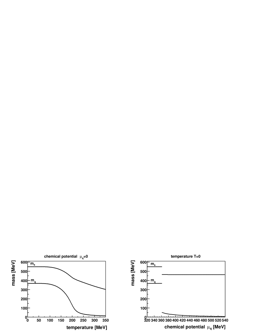
At zero density we observe a smooth cross-over of the chiral phase transition as a function of temperature: at low temperature the chiral symmetry is spontaneously broken, with rising temperature the quark condensate melts away and the quark masses approach the current mass, at least for the light quarks. For the strange quarks we observe a much smoother transition and at the highest temperature we can treat in the framework of the NJL model (approximately $230\,MeV$) their mass is still higher than their current mass . This smooth cross-over we observe only for the special case of three non-zero current quark masses.

At zero temperature we observe for our parameter set a first order phase transition. As a function of the chemical potential the light quark mass drops suddenly to a value close to the current quark mass. The strange quarks change slightly their mass due to the coupling between the flavors. For higher values of the chemical potential the strange quark mass is stable. The light quark condensate is too small for a change of the strange quark mass. Only a rise of the chemical potential of the strange quarks can drop the strange quark mass further, as will be discussed in the last part of this section where we present the extension to strange quark matter.

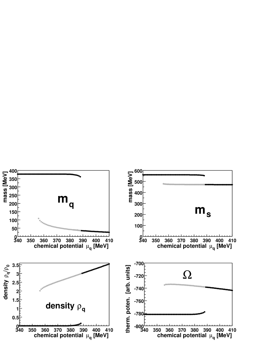
A first order phase transition is characterized by the existence of metastable phases, the equivalent of for example oversaturated vapor. These metastable phases are a solution of the gap equation, but their thermodynamical potential is larger than for the stable phase. We show this in detail in figureย 2. On the top we display the quark mass (light and strange), on the bottom the density of light quarks and the thermodynamical potential. The stable phases which minimize the thermodynamical potential are shown as dark lines, the metastable phases as light lines.

For the mass of the light quarks we observe the transition from the stable phase at high chemical potential to a state whose mass is larger than its chemical potential, this means to zero density. Increasing the chemical potential yields a first order phase transition, i.e. the mass of the quarks drops suddenly. This abrupt change in the quark masses gives rise to a jump in the density - for a constant chemical potential suddenly much more states become accessible. This implies at the same time that certain densities does not exist.

Refer to caption
Figure 2: Detailed representation of the first order phase transition as a function of the light quark potential at zero temperature. On the top: the light (lhs) and strange (rhs) quark masses bottom: the density (lhs) and the thermodynamical potential (rhs). The light lines represent the metastable region, the dark lines the stable region (minimization of the thermodynamical potential).

In our case the normal nuclear matter density is just in this region and there are nice explications for this fact [27][3]. For the interpretation one has to remember that we are talking about a quark gas without confinement. Here, nuclear matter at normal density one has to consider as a phase which contains dense droplets of quarks in which chiral symmetry is restored, surrounded by the vacuum or a very diluted quark gas (which should be confined in QCD). The size of these droplets is not given by the theory, but it is not farfetched to identify these objects with the nucleons.

We observe thus for our set of parameters a first order phase transition as a function of the chemical potential at zero temperature and cross-over as a function of temperature at zero density. Extrapolating now to the plane of finite temperature and chemical potential there must be a point where both kinds of phase transition join, the so called tricritical point. In figureย 3 we show this phase diagram at finite temperatures and chemical potentials (lhs, at the rhs as a function of density). We display as dark lines the transition by the stable state (or the transition line for the cross-over) and as light lines the metastable phases. The tricritical point is located at a temperature $T=66\,MeV$ and a chemical potential of $\mu_{q}=321\,MeV$ which corresponds to a density of $\rho_{q}=1.88\rho_{0}$.

Refer to caption
Figure 3: Phase diagram for the mass of the light quarks (chiral phase transition) as a function of temperature and the light quark chemical potential (lhs) and density (rhs). The dark lines represent the transition by the stable phases, the light lines the transition by metastable phases in case of a first order phase transition.

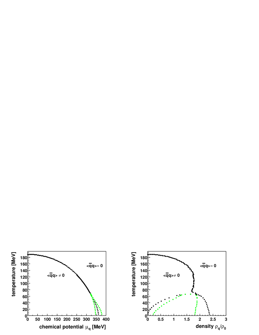
The location of the tricritical point depends strongly on the choice of the cut-off and of the coupling constant [28].
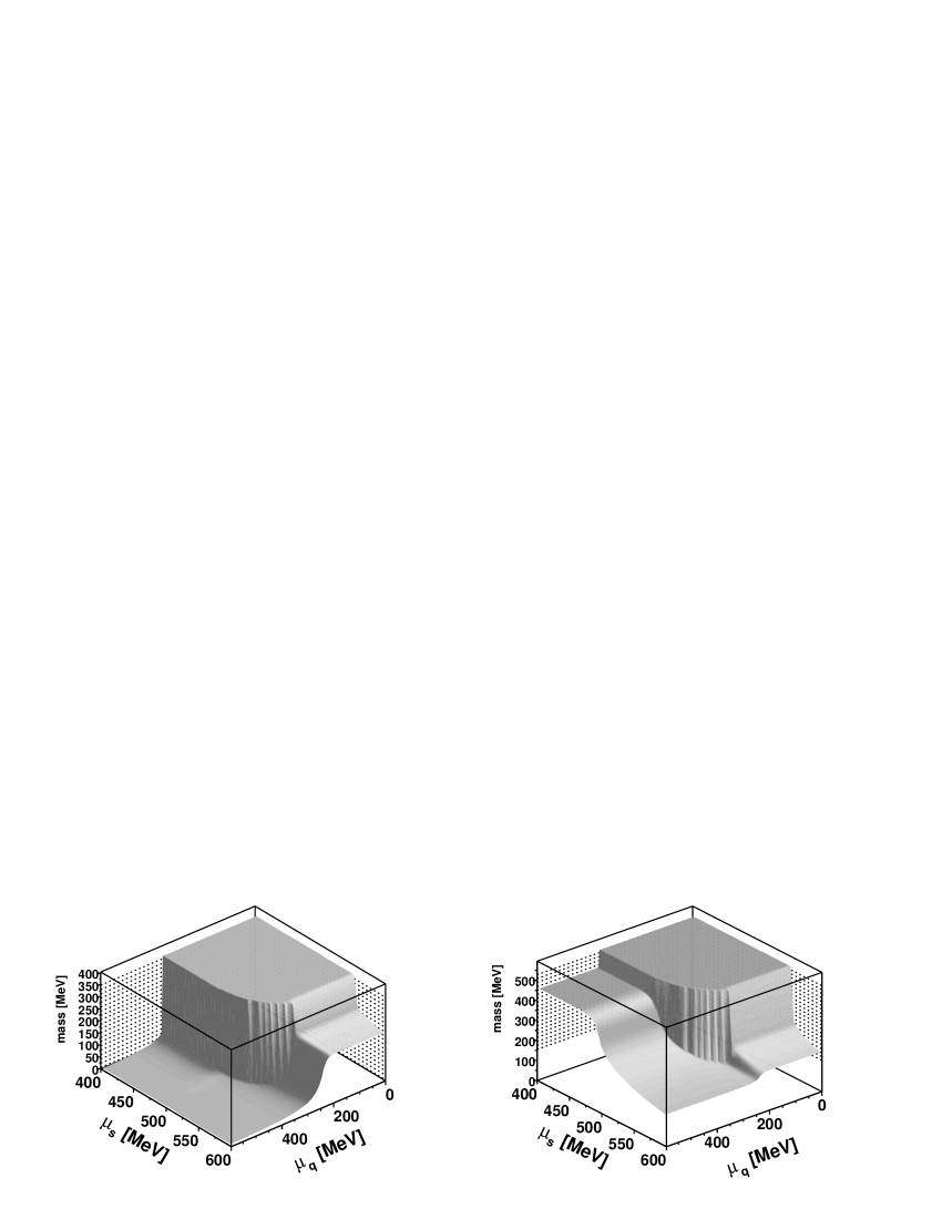
In figureย 4 we plot the quark masses (light, lhs and strange, rhs) as a function of the chemical potential of light and strange quarks at zero temperature. We can see the influence of the coupling between the flavors as already discussed for the light quark chemical potential. The strange quark mass drops suddenly at high chemical potentials of the strange quarks ฮผssubscript๐œ‡๐‘ \mu_{s} and low chemical potentials for the light quarks $\mu_{q}$. Once the chiral phase transition for the light quarks has taken place (at high values of $\mu_{q}$), the strange quark mass shows a cross-over transition for high ฮผssubscript๐œ‡๐‘ \mu_{s}. For high values of $\mu_{q}$ and ฮผssubscript๐œ‡๐‘ \mu_{s}, both quark masses have a value close to their current quark mass.

Refer to caption
Figure 4: Light (lhs) and strange (rhs) quark masses as a function of the chemical potential of light ($\mu_{q}$) and strange (ฮผssubscript๐œ‡๐‘ \mu_{s}) quarks at zero temperature.

With increasing temperature, the phase transitions will take place at lower values of the chemical potentials. This is very pronounced for the light quarks (see figureย 1) and less for the strange quarks which change their mass quite slowly with temperature due to the high current quark mass (compare figureย 1).

3 Color superconductivity

In this section we will study the diquark channel. We will see that quarks which have opposite spin and momenta condense in the scalar channel into diquarks. This resembles superconductivity [23][24]. Here we have in addition a complex structure in color and flavor space. In classical superconductivity the condensation occurs close to the Fermi surface. In our case we have to take into account that quarks with different flavors may have different Fermi-surfaces. Because the coupling between the quarks is quite small, the condensation will only occur if the Fermi momenta of the two quarks are quite close to each other.

In order to calculate the properties of the NJL model in the superconducting sector, we will apply the generalized thermodynamical approach of the Hartree-Bogolyubov theory to quark matter (see for example [26]) described by the Lagrangian (1).

The Lagrangian (1) in the mean field approximation including the diquark sector reads as follows:

$\displaystyle\mathscr{L}^{MF}$ $\displaystyle=$ $\displaystyle\sum\bar{q}(i{\partial}\!\!\!{/}-M)q-2G_{S}(\alpha^{2}+\beta^{2}+\gamma^{2})+4G_{D}\alpha\beta\gamma$ (15)
+qยฏiโ€‹ฮฑโ€‹ฮ”~kโ€‹ฮณ2โ€‹qjโ€‹ฮฒC+qยฏiโ€‹ฮฑCโ€‹ฮ”~kโ€‹ฮณโฃโ€ 2โ€‹qjโ€‹ฮฒโˆ’โˆ‘k,ฮณ|ฮ”kโ€‹ฮณ|24โ€‹GDโ€‹Iโ€‹Qsubscriptยฏ๐‘ž๐‘–๐›ผsuperscript~ฮ”๐‘˜๐›พ2superscriptsubscript๐‘ž๐‘—๐›ฝ๐ถsuperscriptsubscriptยฏ๐‘ž๐‘–๐›ผ๐ถsuperscript~ฮ”๐‘˜๐›พโ€ 2subscript๐‘ž๐‘—๐›ฝsubscript๐‘˜๐›พsuperscriptsuperscriptฮ”๐‘˜๐›พ24subscript๐บ๐ท๐ผ๐‘„\displaystyle+\bar{q}_{i\alpha}\frac{\tilde{\Delta}^{k\gamma}}{2}q_{j\beta}^{C}+\bar{q}_{i\alpha}^{C}\frac{\tilde{\Delta}^{k\gamma\dagger}}{2}q_{j\beta}-\sum_{k,\gamma}\frac{|\Delta^{k\gamma}|^{2}}{4G_{DIQ}}

greek indices denote the colors, latin indices the flavors.

The diquark condensate is defined by:

$$\tilde{\Delta}^{k\gamma}=2G_{DIQ}i\gamma_{5}\epsilon^{\alpha\beta\gamma}\epsilon^{ijk}\langle\!\langle\bar{q}_{i^{\prime}\alpha^{\prime}}i\gamma_{5}\epsilon^{i^{\prime}j^{\prime}k}\epsilon^{\alpha^{\prime}\beta^{\prime}\gamma}q_{j^{\prime}\beta^{\prime}}^{C}\rangle\!\rangle=i\gamma_{5}\epsilon^{\alpha\beta\gamma}\epsilon^{ijk}\Delta^{k\gamma}$$ (16)

This diquark condensate occurs for all three colors simultaneously. We note that as in classical superconductivity the baryon (or particle) number is not conserved. Hence the electromagnetic $U_{em}(1)$ symmetry is spontaneously broken and Goldstone bosons appear in the form of Cooper pairs. The diquark condensate carries a color and a flavor index. For a given flavor and color the condensate is completely antisymmetric in the two other flavors and colors. The condensate ฮ”sโ€‹rsuperscriptฮ”๐‘ ๐‘Ÿ\Delta^{sr} is created for example by green and blue up and down quarks.

The diquark condensate is completely antisymmetric in the color degrees of freedom, a property which is only shared by three of the eight Gell Mann matrices which generate the $SU_{C}(3)$. Hence a finite diquark condensate breaks down the $SU_{C}(3)$ color symmetry to a $SU_{C}(2)$ if the mass of the strange quark is heavy. The same is true for the flavor sector if the three flavors are degenerated in mass. For two flavors only the Lagrangian is invariant with respect to a chiral transformation. If the diquark condensates coexist for all three flavors, the chiral symmetry is spontaneously broken.

Due to the product of two antisymmetric tensors the symmetry is even more reduced if all three quark flavors form a diquark condensate. In order to see this, we assume first that all three colors (for one flavor) are equivalent. Than we can assume without loss of generality that $k=\gamma$ in equation (16) and write the tensor product as:

$$\epsilon^{ijI}\epsilon^{\alpha\beta I}=\sum_{i,j,\alpha,\beta}(\delta_{i,\alpha}\delta_{j,\beta}-\delta_{i,\beta}\delta_{j,\alpha})$$ (17)

We see that in this case the rotations in color and flavor space are no longer independent but locked. Hence the quarks are in a color-flavor locked phase if all three quark flavors participate at the formation of the diquark condensates. $\delta_{i,\alpha}$ is the unit matrix of $SU(3)_{C\times F}$ in which the matrices contain as columns the three flavors and as rows the three colors. The Lagrangian is therefore invariant under a $SU(3)_{C\times F}$ transformation and consequently the $SU(3)$ color and flavor symmetries are reduced to an $SU(3)_{C\times F}$ symmetry. For more consequences of the appearance of the condensate for the symmetries we refer to the literature [12]. Here we will focus on a numerical evaluation of the size of the condensates and the phase transitions at finite temperature and density.

3.1 Thermodynamics

As before in the case of the chiral phase transition we will evaluate all condensates and the phase diagram by the evaluation of the thermodynamical potential.

We start by writing the Lagrangian in a more symmetric form, following Nambu who developed this formalism for the classical superconductivity [25]. For this purpose we rewrite the Lagrangian as a sum of the original Lagrangian and its charge conjugate:

$$\mathscr{L}_{Nambu}=\mathscr{L}+\mathscr{L}^{C}$$ (18)

Then the Lagrangian can be presented as a matrix:

โ„’Nโ€‹aโ€‹mโ€‹bโ€‹uMโ€‹F=[12โ€‹qยฏ12โ€‹qยฏC]โ€‹[iโˆ‚/โˆ’Mfฮ”~kโ€‹ฮณโฃโ€ ฮ”~kโ€‹ฮณโˆ’iโˆ‚/Tโˆ’Mf]โ€‹[12โ€‹q12โ€‹qC]+โ„’cโ€‹oโ€‹nโ€‹d\mathscr{L}_{Nambu}^{MF}=\left[\begin{array}[]{cc}\frac{1}{\sqrt{2}}\bar{q}&\frac{1}{\sqrt{2}}\bar{q}^{C}\end{array}\right]\left[\begin{array}[]{cc}i{\partial}\!\!\!{/}-M_{f}&\tilde{\Delta}^{k\gamma\dagger}\\ \tilde{\Delta}^{k\gamma}&-i{\partial}\!\!\!{/}^{T}-M_{f}\end{array}\right]\left[\begin{array}[]{c}\frac{1}{\sqrt{2}}q\\ \frac{1}{\sqrt{2}}q^{C}\end{array}\right]+\mathscr{L}_{cond} (19)

where we suppressed the indices for convenience and defined the term

$$\mathscr{L}_{cond}=-2G_{S}(\alpha^{2}+\beta^{2}+\gamma^{2})+4G_{D}\alpha\beta\gamma+\frac{|\Delta^{k\gamma}|^{2}}{4G_{DIQ}}.$$ (20)

In order to calculate the thermodynamical potential in this notation

$$\Omega=-\beta Tr[\ln exp(-\beta(\hat{H}_{Nambu}-\mu\hat{N}-\mu\hat{N}^{C}))]$$

we need the particle number operator and its charge conjugate:

N^=โˆ‘pโ†’,s,f,c[a^pโ†’,sโ€ โ€‹a^pโ†’,sโˆ’b^pโ†’,sโ€ โ€‹b^pโ†’,s]N^C=โˆ’โˆ‘pโ†’,s,f,c[a^pโ†’,sโ€‹a^pโ†’,sโ€ โˆ’b^pโ†’,sโ€‹b^pโ†’,sโ€ ]formulae-sequence^๐‘subscriptโ†’๐‘๐‘ ๐‘“๐‘delimited-[]superscriptsubscript^๐‘Žโ†’๐‘๐‘ โ€ subscript^๐‘Žโ†’๐‘๐‘ superscriptsubscript^๐‘โ†’๐‘๐‘ โ€ subscript^๐‘โ†’๐‘๐‘ superscript^๐‘๐ถsubscriptโ†’๐‘๐‘ ๐‘“๐‘delimited-[]subscript^๐‘Žโ†’๐‘๐‘ superscriptsubscript^๐‘Žโ†’๐‘๐‘ โ€ subscript^๐‘โ†’๐‘๐‘ superscriptsubscript^๐‘โ†’๐‘๐‘ โ€ \hat{N}=\sum_{\vec{p},s,f,c}\left[\hat{a}_{\vec{p},s}^{\dagger}\hat{a}_{\vec{p},s}-\hat{b}_{\vec{p},s}^{\dagger}\hat{b}_{\vec{p},s}\right]\quad\hat{N}^{C}=-\sum_{\vec{p},s,f,c}\left[\hat{a}_{\vec{p},s}\hat{a}_{\vec{p},s}^{\dagger}-\hat{b}_{\vec{p},s}\hat{b}_{\vec{p},s}^{\dagger}\right] (21)

where we suppressed the explicit dependence of the operators on flavor and color degrees of freedom.

When calculating the Hamiltonian in the mean field approximation, one can see that it is possible to separate $\hat{H}-\mu\hat{N}$ into two parts, one for the quarks (operators $\hat{a}$ and a^โ€ superscript^๐‘Žโ€ \hat{a}^{\dagger}) and another for the antiquarks (operators $\hat{b}$ et b^โ€ superscript^๐‘โ€ \hat{b}^{\dagger}):

$$\hat{H}-\mu\hat{N}=(\hat{H}-\mu\hat{N})_{\hat{a}}+(\hat{H}-\mu\hat{N})_{\hat{b}}$$ (22)

These two parts yield the explicit expressions

(H^โˆ’ฮผโ€‹N^)a^=โˆ‘pโ†’,s,f,c[a^pโ†’,sโ€ a^โˆ’pโ†’,โˆ’s]โ€‹[Epโ†’,fโˆ’ฮผfโˆ’ฮ”~kโ€‹ฮณโฃโ€ โ€‹Nโ€‹(p)ฮ”~kโ€‹ฮณโ€‹Nโ€‹(p)โˆ’Epโ†’,f+ฮผf]โ€‹[a^pโ†’,sa^โˆ’pโ†’,โˆ’sโ€ ]+Hcโ€‹oโ€‹nโ€‹dsubscript^๐ป๐œ‡^๐‘^๐‘Žsubscriptโ†’๐‘๐‘ ๐‘“๐‘delimited-[]subscriptsuperscript^๐‘Žโ€ โ†’๐‘๐‘ subscript^๐‘Žโ†’๐‘๐‘ delimited-[]subscript๐ธโ†’๐‘๐‘“subscript๐œ‡๐‘“superscript~ฮ”๐‘˜๐›พโ€ ๐‘๐‘superscript~ฮ”๐‘˜๐›พ๐‘๐‘subscript๐ธโ†’๐‘๐‘“subscript๐œ‡๐‘“delimited-[]subscript^๐‘Žโ†’๐‘๐‘ subscriptsuperscript^๐‘Žโ€ โ†’๐‘๐‘ subscript๐ป๐‘๐‘œ๐‘›๐‘‘(\hat{H}-\mu\hat{N})_{\hat{a}}=\sum_{\vec{p},s,f,c}\left[\begin{array}[]{cc}\hat{a}^{\dagger}_{\vec{p},s}&\hat{a}_{-\vec{p},-s}\end{array}\right]\left[\begin{array}[]{cc}E_{\vec{p},f}-\mu_{f}&-\tilde{\Delta}^{k\gamma\dagger}N(p)\\ \tilde{\Delta}^{k\gamma}N(p)&-E_{\vec{p},f}+\mu_{f}\end{array}\right]\left[\begin{array}[]{c}\hat{a}_{\vec{p},s}\\ \hat{a}^{\dagger}_{-\vec{p},-s}\end{array}\right]+H_{cond} (23)

and

(H^โˆ’ฮผโ€‹N^)b^=โˆ‘pโ†’,s,f,c[b^pโ†’,sโ€ b^โˆ’pโ†’,โˆ’s]โ€‹[Epโ†’,f+ฮผfโˆ’ฮ”~kโ€‹ฮณโฃโ€ โ€‹Nโ€‹(p)ฮ”~kโ€‹ฮณโ€‹Nโ€‹(p)โˆ’Epโ†’,fโˆ’ฮผf]โ€‹[b^pโ†’,sb^โˆ’pโ†’,โˆ’sโ€ ]+Hcโ€‹oโ€‹nโ€‹d.subscript^๐ป๐œ‡^๐‘^๐‘subscriptโ†’๐‘๐‘ ๐‘“๐‘delimited-[]subscriptsuperscript^๐‘โ€ โ†’๐‘๐‘ subscript^๐‘โ†’๐‘๐‘ delimited-[]subscript๐ธโ†’๐‘๐‘“subscript๐œ‡๐‘“superscript~ฮ”๐‘˜๐›พโ€ ๐‘๐‘superscript~ฮ”๐‘˜๐›พ๐‘๐‘subscript๐ธโ†’๐‘๐‘“subscript๐œ‡๐‘“delimited-[]subscript^๐‘โ†’๐‘๐‘ subscriptsuperscript^๐‘โ€ โ†’๐‘๐‘ subscript๐ป๐‘๐‘œ๐‘›๐‘‘(\hat{H}-\mu\hat{N})_{\hat{b}}=\sum_{\vec{p},s,f,c}\left[\begin{array}[]{cc}\hat{b}^{\dagger}_{\vec{p},s}&\hat{b}_{-\vec{p},-s}\end{array}\right]\left[\begin{array}[]{cc}E_{\vec{p},f}+\mu_{f}&-\tilde{\Delta}^{k\gamma\dagger}N(p)\\ \tilde{\Delta}^{k\gamma}N(p)&-E_{\vec{p},f}-\mu_{f}\end{array}\right]\left[\begin{array}[]{c}\hat{b}_{\vec{p},s}\\ \hat{b}^{\dagger}_{-\vec{p},-s}\end{array}\right]+H_{cond.} (24)

We denoted by $H_{cond}$ the expression $-V*\mathscr{L}_{cond}$ and used here the discrete summation over the momenta. The expressions have a defined structure in flavor and color, the diagonal terms are diagonal in flavor and color, the off-diagonal terms ($\tilde{\Delta}$) are antisymmetric in color and flavor and

$\displaystyle N(p)_{f_{1},f_{2}}$ $\displaystyle=$ $\displaystyle\left(1+\frac{p^{2}}{(E_{f_{1}}+m_{f_{1}})(E_{f_{2}}+m_{f_{2}})}\right)$ (25)
$\displaystyle\times$ $\displaystyle\sqrt{\frac{(E_{f_{1}}+m_{f_{1}})(E_{f_{2}}+m_{f_{2}})}{{4m_{f_{1}}m_{f_{2}}}}}\sqrt{\frac{m_{f_{1}}m_{f_{2}}}{E_{f_{1}}E_{f_{2}}}}$

This normalization factor is due to the fact that we deal with products of spinors for different species in the off diagonal terms, of course $N(p)=1$ when $f_{1}=f_{2}$. The explicit form of this matrix including all flavor and color indices is displayed in appendix C.

In order to calculate the thermodynamical potential, we have to diagonalize these expressions. This has to be done by means of a Bogolyubov transformation which determines the energies of the quasi-particles and the corresponding quasi-particle operators. From the discussion of the symmetry of the diquark condensate we expect two quarks of different flavor and color to form a diquark condensate whereas one quark of the third flavor is not involved in forming this condensate. This has to be seen in the quasi-particle energy and is confirmed if we evaluate explicitly the quasi-particle energies as the eigenvalues of the matrices. The diagonalized operators corresponding to $(\hat{H}-\mu\hat{N})_{\hat{a}}$ can be expressed in the form:

(H^โˆ’ฮผโ€‹N^)a^ฮ”=โˆ‘i,ฮฑ=13(Eiโ€‹ฮฑโ€‹a^ฮ”โ€‹iโ€‹ฮฑโ€ โ€‹a^ฮ”โ€‹iโ€‹ฮฑ+Eiโ€‹ฮฑโ€ฒโ€‹a^ฮ”โ€‹iโ€‹ฮฑโ€‹a^ฮ”โ€‹iโ€‹ฮฑโ€ )subscript^๐ป๐œ‡^๐‘subscript^๐‘Žฮ”subscriptsuperscript3๐‘–๐›ผ1subscript๐ธ๐‘–๐›ผsubscriptsuperscript^๐‘Žโ€ ฮ”๐‘–๐›ผsubscript^๐‘Žฮ”๐‘–๐›ผsuperscriptsubscript๐ธ๐‘–๐›ผโ€ฒsubscript^๐‘Žฮ”๐‘–๐›ผsubscriptsuperscript^๐‘Žโ€ ฮ”๐‘–๐›ผ(\hat{H}-\mu\hat{N})_{\hat{a}_{\Delta}}=\sum^{3}_{i,\alpha=1}(E_{i\alpha}\hat{a}^{\dagger}_{\Delta i\alpha}\hat{a}_{\Delta i\alpha}+E_{i\alpha}^{\prime}\hat{a}_{\Delta i\alpha}\hat{a}^{\dagger}_{\Delta i\alpha})

where $i$ runs over the flavors and $\alpha$ over the colors. $\hat{a}_{\Delta i\alpha}$ and a^ฮ”โ€‹iโ€‹ฮฑโ€ subscriptsuperscript^๐‘Žโ€ ฮ”๐‘–๐›ผ\hat{a}^{\dagger}_{\Delta i\alpha} are annihilation and creation operators for the quasi particles. :

i $E_{a},i$ $g_{i}$
1 $\pm\sqrt{\Delta_{qq}+{E^{-}}^{2}}$ 3
2 ยฑ12โ€‹(Z+Eโˆ’โˆ’Esโˆ’)plus-or-minus12๐‘superscript๐ธsubscriptsuperscript๐ธ๐‘ \pm\frac{1}{2}({Z}+E^{-}-E^{-}_{s}) 2
3 ยฑ12โ€‹(Zโˆ’Eโˆ’+Esโˆ’)plus-or-minus12๐‘superscript๐ธsubscriptsuperscript๐ธ๐‘ \pm\frac{1}{2}({Z}-E^{-}+E^{-}_{s}) 2
4 $\sqrt{Y-X}$ 1
5 $\sqrt{Y+X}$ 1

where

$\displaystyle E^{-}$ $\displaystyle=$ $\displaystyle E-\mu$ (26)
Esโˆ’subscriptsuperscript๐ธ๐‘ \displaystyle E^{-}_{s} $\displaystyle=$ Esโˆ’ฮผssubscript๐ธ๐‘ subscript๐œ‡๐‘ \displaystyle E_{s}-\mu_{s} (27)
$\displaystyle Z$ $\displaystyle=$ 4โ€‹ฮ”qโ€‹sโ€‹N2โ€‹(p)+(Eโˆ’+Esโˆ’)24subscriptฮ”๐‘ž๐‘ superscript๐‘2๐‘superscriptsuperscript๐ธsubscriptsuperscript๐ธ๐‘ 2\displaystyle\sqrt{4\Delta_{qs}N^{2}(p)+(E^{-}+E^{-}_{s})^{2}} (28)
$\displaystyle Y$ $\displaystyle=$ 12โ€‹(ฮ”qโ€‹q2+4โ€‹ฮ”qโ€‹s2โ€‹N2โ€‹(p)+Eโˆ’2+Esโˆ’2)12superscriptsubscriptฮ”๐‘ž๐‘ž24superscriptsubscriptฮ”๐‘ž๐‘ 2superscript๐‘2๐‘superscriptsuperscript๐ธ2superscriptsubscriptsuperscript๐ธ๐‘ 2\displaystyle\frac{1}{2}\left(\Delta_{qq}^{2}+4\Delta_{qs}^{2}N^{2}(p)+{E^{-}}^{2}+{E^{-}_{s}}^{2}\right) (29)
$\displaystyle X^{2}$ $\displaystyle=$ $\displaystyle\frac{1}{4}\Bigl{(}\Delta_{qq}^{2}+(8\Delta_{qs}^{2}N^{2}(p)+(E^{-}+E_{s}^{-})^{2})(E^{-}-E_{s}^{-})^{2}$ (30)
$\displaystyle+$ $\displaystyle 2\Delta_{qq}^{2}\bigl{(}4\Delta_{qs}^{2}N^{2}(p)+(E^{-}+E_{s}^{-})(E^{-}-E_{s}^{-})\bigr{)}\Bigr{)}$

and $g_{i}$ is the degeneracy. For the calculation of the thermodynamical potential it is not necessary to know the exact form of the Bogolyubov transformation which relates the quasi particle operators $\hat{a}_{\Delta}$ with the original quark operators $\hat{a}$. The quasi-particles are still fermions, and that is all information we need in order to evaluate the sum over the occupied states. It is just necessary to assign the right energies to the operators. We evaluate the thermodynamical potential for the case of two degenerated light quarks:

$\displaystyle\frac{\Omega}{V}=\frac{\Omega_{0}}{V}-\frac{2}{\beta}\int^{\Lambda}_{0}\frac{d\vec{p}}{(2\pi)^{3}}$ $\displaystyle\Bigl{\{}$ $\displaystyle 6\ln[1+\exp(-\beta E_{1-})]$
$\displaystyle+$ $\displaystyle 4\ln[1+\exp(-\beta E_{2-})]$
$\displaystyle+$ $\displaystyle 4\ln[1+\exp(-\beta E_{3-})]$
$\displaystyle+$ $\displaystyle 2\ln[1+\exp(-\beta E_{4-})]$
$\displaystyle+$ $\displaystyle 2\ln[1+\exp(-\beta E_{5-})]$
$\displaystyle+3\beta E_{1-}+2\beta E_{2-}$ $\displaystyle+$ $\displaystyle 2\beta E_{3-}+\beta E_{4-}+\beta E_{5-}\Bigl{\}}$ (31)

with

ฮฉ0V=4โ€‹GSโ€‹(ฮฑ2+ฮฒ2+ฮณ2)+2โ€‹|ฮ”qโ€‹s|2+|ฮ”qโ€‹q|22โ€‹GDโ€‹Iโ€‹Qsubscriptฮฉ0๐‘‰4subscript๐บ๐‘†superscript๐›ผ2superscript๐›ฝ2superscript๐›พ22superscriptsubscriptฮ”๐‘ž๐‘ 2superscriptsubscriptฮ”๐‘ž๐‘ž22subscript๐บ๐ท๐ผ๐‘„\frac{\Omega_{0}}{V}=4G_{S}(\alpha^{2}+\beta^{2}+\gamma^{2})+\frac{2|\Delta_{qs}|^{2}+|\Delta_{qq}|^{2}}{2G_{DIQ}} (32)

This thermodynamical potential contains the (quark and diquark) condensates as parameters. In order to evaluate them, we have to minimize

$$\frac{\partial\Omega}{\partial\langle\!\langle\bar{q}_{f}q_{f}\rangle\!\rangle}=0\qquad\frac{\partial\Omega}{\partial\Delta_{f_{1}f_{2}}}=0.$$ (33)

This minimization yields the gap equations for the quark condensates. For the SU(3) case the derivation is given in the appendix D. These equations are coupled, we have to solve them selfconsistently. The resulting $<qq>$ condensates may be found in appendix E.

3.2 Results at finite temperature and density

For this part we decide to take parameter in ref. [30] :$m_{0,q}=5.96MeV$, $\Lambda=592.7MeV$, $G_{S}=6.92GeV^{-2}$, $G_{DIQ}/G_{S}=3./4.$ and m0,s=130.7โ€‹Mโ€‹eโ€‹Vsubscript๐‘š0๐‘ 130.7๐‘€๐‘’๐‘‰m_{0,s}=130.7MeV. We use the relation between the coupling constants, ( $G_{DIQ}=3G_{S}/4$ ), given by the Fierz-transformation (see appendix A), close to [30] (0.73).

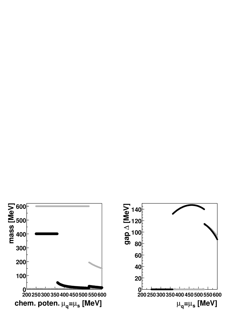
The condensates resp. masses at zero temperature as a function of the chemical potential ฮผq=ฮผssubscript๐œ‡๐‘žsubscript๐œ‡๐‘ \mu_{q}=\mu_{s} are displayed in figureย 5. On the lhs of this figure we show the light and strange quark mass, on the rhs the diquarks condensates. First we have to note that quark and diquark condensates compete with each other as they are formed by the same quarks. Temperature and density determine which condensate dominates.

When the chiral phase transition occurs (the quark condensate disappears), we observe for the light quarks that the superconducting phase transition takes place and we have a diquark condensate. As the two transitions are related, they are of the same order. The same scenario repeats itself for the strange diquark condensate at a higher chemical potential. In the figure we display only the solution which is the global minimum of the thermodynamical potential.

At a quite low chemical potential (the light quarks have a very small mass, the strange quarks are heavy) we have only the light diquark condensate, the diquark condensate including strange quarks is almost zero as the strange quarks show a strong quark condensate. Only when the strange quark condensate drops and the mass of the strange quarks approaches its current mass, the strange diquark condensate appears. We have here the coexistence of the light and strange diquark condensate, this is the regime where the chiral symmetry is broken again and color and flavor are locked. This happens at a quite high chemical potential, the decreasing diquark condensate for even higher chemical potentials indicates that we reach the limit of the model: we are too close to the cut-off. The phase transitions concerning the strange quarks are quite close to the limits of the models if we suppose the current mass of the strange quark of around $140\,MeV$. We note that due to the relatively small difference between the quark masses, both diquark condensates have approximately the same value, for the maximum we get ฮ”qโ€‹qโ‰ˆฮ”qโ€‹sโ‰ˆ(120โ€‹Mโ€‹eโ€‹V)3subscriptฮ”๐‘ž๐‘žsubscriptฮ”๐‘ž๐‘ superscript120๐‘€๐‘’๐‘‰3\Delta_{qq}\approx\Delta_{qs}\approx(120\,MeV)^{3}.

Refer to caption
Figure 5: The light (dark line) and strange (light line) quark masses and the diquark condensates $\Delta_{qq}$ (dark line) and ฮ”qโ€‹ssubscriptฮ”๐‘ž๐‘ \Delta_{qs} (light line) as a function of the chemical potential ฮผq=ฮผssubscript๐œ‡๐‘žsubscript๐œ‡๐‘ \mu_{q}=\mu_{s} at zero temperature.

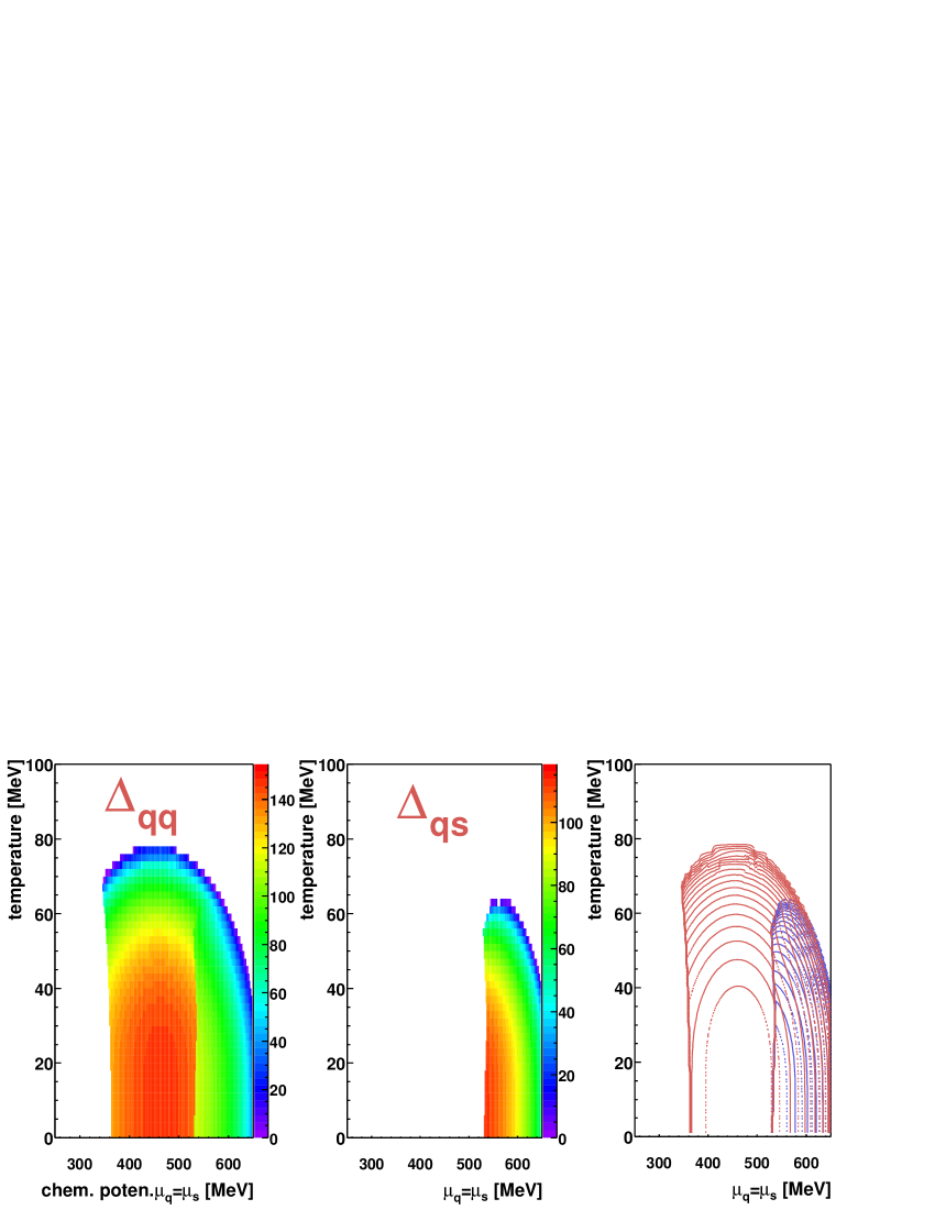
At zero temperature the chiral phase transition (where the quark condensates disappear) and the superconducting phase transition (where the diquark condensates appear) are strongly related in of our model. This changes at higher temperatures. There the diquark condensates $\Delta_{qq}$ extends to smaller values of the chemical potential whereas we need higher densities in order to form a ฮ”qโ€‹ssubscriptฮ”๐‘ž๐‘ \Delta_{qs} diquark condensate. In addition the diquark condensate become smaller with increasing temperature. This is shown in figureย 6 where we plot the diquark condensates as a function of temperature and chemical potential. For a given chemical potential we observe - as in the classical superconductivity - a second order phase transition as a function of the temperature.

Refer to caption
Figure 6: Strength of the diquark condensates as a function of the chemical potential ฮผq=ฮผssubscript๐œ‡๐‘žsubscript๐œ‡๐‘ \mu_{q}=\mu_{s} and the temperature. We show as color-levels the strength of the condensates $\Delta_{qq}$ (lhs), ฮ”qโ€‹ssubscriptฮ”๐‘ž๐‘ \Delta_{qs} (middle) and superimpose both as a contour plot (rhs).

In a next step we consider the diquark condensates in the ฮผqโˆ’ฮผssubscript๐œ‡๐‘žsubscript๐œ‡๐‘ \mu_{q}-\mu_{s} plane. As already mentioned, we expect the formation of a diquark condensate only if there are quarks with similar Fermi momentum, independent of their mass. Because $G_{D}$ is zero the disappearance of the quark condensates <sโ€‹sยฏ>expectation๐‘ ยฏ๐‘ <s\bar{s}> and $<q\bar{q}>$ does not depend on the chemical potential of the other species. There is one exception the creation of the strange diquark condensates lowers the strange quark condensate and increases the light quark mass. In figureย 7 we plot the strength of the diquark condensates. Because both light quarks have the same chemical potential a diquark condensate $\Delta_{qq}$ between the two different flavors occurs whenever the light quark mass is small.

Refer to caption
Figure 7: As a function of the chemical potential $\mu_{q}$ and ฮผssubscript๐œ‡๐‘ \mu_{s} we show the quark masses on the upper row (light quarks lhs, strange quarks rhs) and the diquark condensates in the lower row ($\Delta_{qq}$ on the lhs and ฮ”qโ€‹ssubscriptฮ”๐‘ž๐‘ \Delta_{qs} on the rhs)

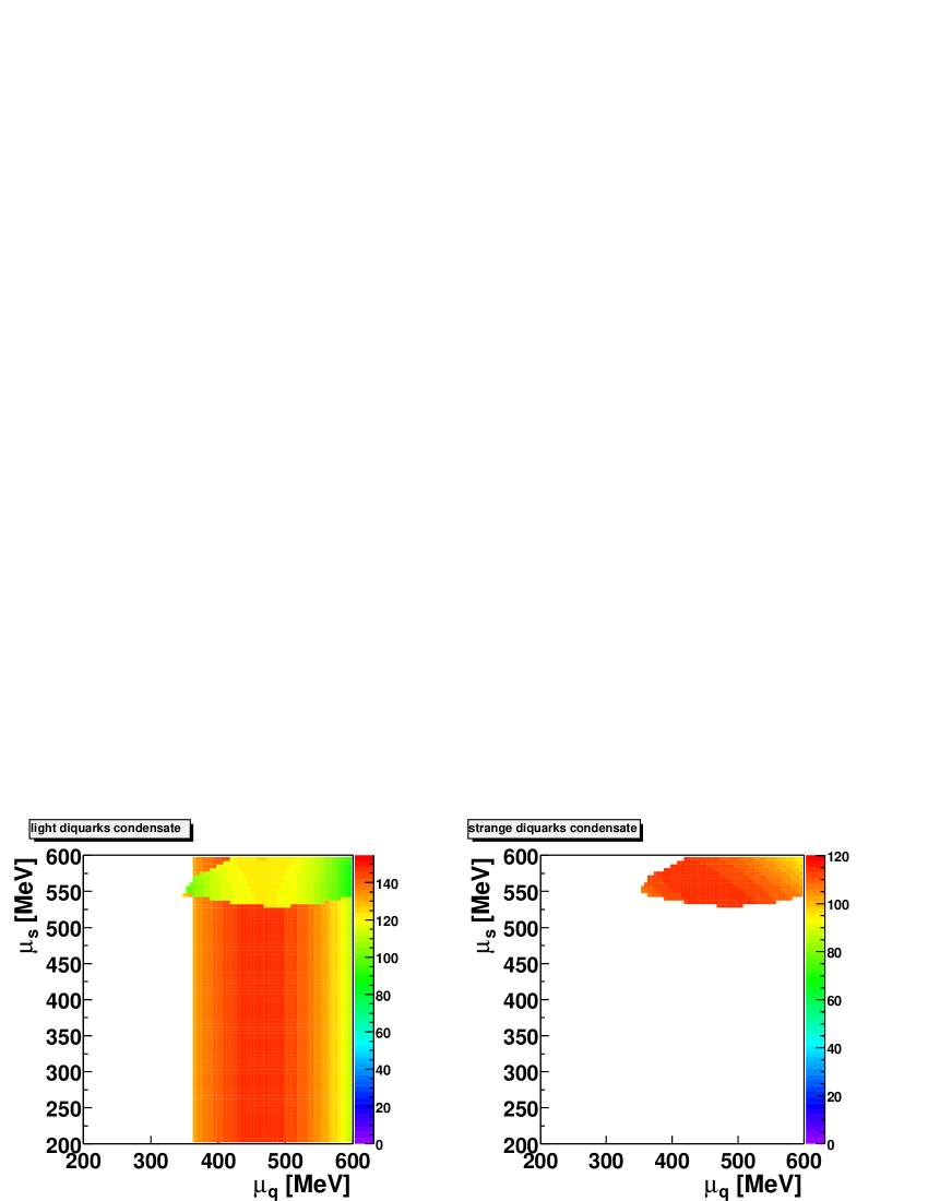
The strange diquark condensate exists only in a band where the chemical potential of the light and strange quarks are approximately equal. The slight deformation of this band is due to the different current quark masses. The width of the band is determined by the coupling strength: if the coupling in the diquark sector is strong, the quarks can bind and form a condensate even if their chemical potentials are quite different. For a small coupling strength, the chemical potentials of the two quarks have to be (approximately, in case of different quark masses) equal in order to form a diquark condensate.

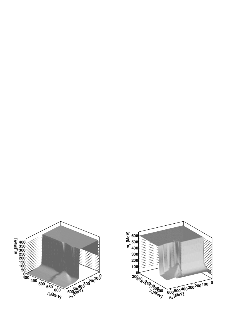
Now we should study the feedback of the formation of the diquark condensates on the quark condensates (or the mass). In 8 we display the masses of the light and strange quarks as a function of $\mu_{q}$ and ฮผssubscript๐œ‡๐‘ \mu_{s}, $\Delta_{qq}$ appears at the chiral phase transition, when the light quark condensate disappears and it is formed by the free light quarks. This behavior is almost independent of ฮผssubscript๐œ‡๐‘ \mu_{s}. Only if ฮ”sโ€‹qsubscriptฮ”๐‘ ๐‘ž\Delta_{sq} becomes finite the lack of quarks for the quark condensate increases the light quark mass. The behavior of ฮ”qโ€‹ssubscriptฮ”๐‘ž๐‘ \Delta_{qs} is generic: When the diquark condensate ฮ”sโ€‹qsubscriptฮ”๐‘ ๐‘ž\Delta_{sq} is finite it takes quarks from the strange quark condensate lowering the mass of the strange quark.

Refer to caption
Figure 8: As a function of the chemical potential $\mu_{q}$ and ฮผssubscript๐œ‡๐‘ \mu_{s} we show the quark masses (light quarks lhs, strange quarks rhs) to pointed out the effect of the diquark condensate on the quark condensate at T=1 MeV.

4 Conclusions

In conclusion, we presented the phase diagram of the $SU(3)$ flavor NJL model extended to the diquark sector for a set of parameters which reproduces meson masses and coupling constants. We find a rich structure of condensates and regions where no condensate exists. The temperature and density dependence of quark and diquark condensates is calculated in mean field approach by minimizing the thermodynamical potential.

The order of chiral phase transition depends on the value of T and $\mu$ where the phase transition occurs. At zero temperature the phase transition is first order and at zero chemical potential we observe a cross over ( due to finite current quark masses). Therefore there exists a tricritical point. Normal nuclear matter density does exist only as a mixed phase of a dense quark phase (where chiral symmetry is partially restored) and a very diluted quark gas or the vacuum (where chiral symmetry is spontaneously broken). Finally we extended the chiral phase transition to the plane of finite strange quark density, relevant for the discussion of the diquark condensates.

Following the idea that the NJL model can be considered as an approximation of the QCD Lagrangian we extend the NJL model by including an interaction in the diquark channel. We find that this interaction gives rise to a diquark condensation which is responsible for the formation of a superconducting gap. This condensation occurs at low temperature and high density. As this gap is formed by two quarks of different flavor, their chemical potential has to be close to each other in order to allow for this condensation. In flavor $SU_{F}(3)$ this condensate breaks the $SU_{F}(3)\times SU_{C}(3)$ down to a $SU_{C\times F}(3)$ a phenomenon which has already been observed in phase diagrams based on instanton Lagrangians and has been dubbed color-flavor locking. We can conclude that two quite differently motivated phenomenological approaches to the QCD Lagrangian provide a very similar phase structure.

The diquark condensates do not exist at temperatures expected to be obtained in relativistic heavy ion collisions. In neutron stars, which have a high density and a very low temperature they could be of relevance.

Acknowledgments

This work was supported by the Landesgraduiertenf rderung Mecklenburg-Vorpommern. One of us (J.A.) acknowledge an interesting discussion with K. Rajagopal. We thank A. W. Steiner and M. Prakash of having pointed out an error in a formula of a previous version of this article.

References

  • [1] B. Barrois Nucl. Phys. B129 (1977) 390
    S. Frautschi, "Proceedings of workshop on hadronic matter at extreme density", Erice 1978
  • [2] D. Bailin, A. Love, Phys. Rept. 107 (1984) 325
  • [3] M. Alford and al. Phys. Lett. B 422 (1998) 247-256
  • [4] R. Rapp, T. Schรคfer, E. Shuryak, M. Velkovsky, Phys. Rev. Lett. 81 (1998) 53.
  • [5] K. Rajagopal; Nucl. Phys. A 661 (1999) 150c-161c
    M. Alford,hep-ph/0102047; To appear in Annu. Rev. Nucl. Part. Sci.
    K. Rajagopal, F Wilczek, hep-ph/0011333; To appear as Chapter 35 in the Festschrift in honor of B. L. Ioffe, "At the Frontier of Particle Physics / Handbook of QCD", M. Shifman, ed., (World Scientific).
    T.Schรคfer, E. Shuryak, nucl-th/0010049,to appear in the proceedings of the ECT Workshop on Neutron Star Interiors, Trento, Italy, June 2000.
  • [6] D. Son, Phys. Rev. D59, 094019 (1999)
    T. Schรคfer, F. Wilczek, Phys. Rev. D60, 114033 (1999)
    R. Pisarski, D.Rischke, Phys. Rev. D61, 074017 (2000)
  • [7] J. Berges, K. Rajagopal; Nucl. Phys. B 538 (1999) 215
  • [8] G. Carter, D. Diakonov, Phys. Rev. D60, 016004 (1999)
  • [9] M. Alford and al. ; Nucl. Phys. B 537 (1999) 443-458
  • [10] M. Asakawa and K. Yazaki; Nucl. Phys. A 504 (1989) 668-684
  • [11] K. Rajagopal; Nucl. Phys. A 642 (1998 ) 26-38
  • [12] T. Sch fer and F. Wilczek; Phys. Rev. Lett. 82 (1999) 3956-3959
  • [13] Y. Nambu, G. Jona-Lasinio; Phys. Rev. 122 (1961) 345-358
  • [14] Y. Nambu, G. Jona-Lasinio; Phys. Rev. 124 (1961) 246-254
  • [15] T.M. Schwarz and al.; Phys. Rev. C 60 (1999) 055205
  • [16] K. Langfeld and M. Rho; Nucl. Phys. A 660 (1999) 475-505
  • [17] T. Hatsuda, T. Kunihiro; Phys. Rep. 247 (1994) 221-367
  • [18] S.P. Klevansky; Rev. Mod. Phys. 64 (1992) 649-708
  • [19] G. Ripka; Quarks Bound by Chiral Fields, Clarendon Press, Oxford, 1997
  • [20] A. Dhar and S. R. Wadia; Phys. Rev. Lett. 52 (1984) 959-962
  • [21] D. Ebert and al.; Prog. Part. Nucl. Phys. 33 (1994) 1-120
  • [22] P. Rehberg and al.; Phys. Rev. C 53 (1996) 410-429
  • [23] J.R. Schrieffer; Theory of Superconductivity, Benjamin, New York, 1964
  • [24] A.F. Fetter, J.D. Walecka; Quantum Theory of Many-Particle Systems; McGraw-Hill, New York, 1971
  • [25] Y. Nambu; Phys. Rev. 117(1960) 648-663
  • [26] M. Iwasaki,, T. Iwado, Progr. Theor. Phys. 94 (1995) 1073
  • [27] M. Bulballa; Nucl. Phys. A 611 (1996) 393-408
  • [28] P.-B. Gossiaux, private communication
  • [29] M. Iwasaki; Prog. Theor. Phys. 100 (1998) 461-464
  • [30] W, Bentz and A.W. Thomas nucl-th/0105022

Appendix A Fierz Transformation

Following Ebert ([21]) we have the following relations in color and flavor space:

$\displaystyle\delta_{ij}\delta_{kl}$ $\displaystyle=$ $\displaystyle\frac{1}{3}\delta_{ik}\delta_{lj}+\frac{1}{2}\sum_{a=1}^{8}\lambda^{a}_{ik}\lambda_{lj}\;\;\;\;\;\;(q\bar{q}\;\;\;\;\;channel)$ (34)
$\displaystyle\delta_{ij}\delta_{kl}$ $\displaystyle=$ $\displaystyle\frac{1}{2}\sum_{a=0}^{8}\lambda^{a}_{il}\lambda^{a}_{kj}\;\;\;\;\;\;(qq\;\;\;\;channel)$ (35)
$\displaystyle\sum_{a=1}^{8}\lambda^{a}_{ij}\lambda^{a}_{kl}$ $\displaystyle=$ $\displaystyle\frac{16}{9}\delta_{il}\delta_{kj}-\frac{1}{3}\sum_{a=1}^{8}\lambda^{a}_{il}\lambda_{kj}\;\;\;\;\;\;(q\bar{q}\;\;\;\;channel)$ (36)
$\displaystyle\sum_{a=1}^{8}\lambda^{a}_{ij}\lambda^{a}_{kl}$ $\displaystyle=$ $\displaystyle\frac{2}{3}\sum_{a=0,1,3,4,6,8}\lambda^{a}_{ik}\lambda^{a}_{lj}-\frac{4}{3}\sum_{a=2,5,7}\lambda^{a}_{ik}\lambda^{a}_{lj}\;\;\;\;\;\;(qq\;\;\;\;channel)$ (37)
$$\mathcal{L}=-g\sum_{a=1}^{8}(\bar{\psi}\gamma^{C}_{\mu}\lambda^{a}\psi)^{2}$$ (38)

This leads to the following relation between the differents coupling constant:

$\displaystyle q\bar{q}\;\;\;\;{\mathsf{channel}}\;\;\;G_{SCA}$ $\displaystyle=$ $\displaystyle\frac{8}{9}g$ (39)
$\displaystyle qq\;\;\;\;{\mathsf{channel}}\;\;\;G_{DIQ}$ $\displaystyle=$ $\displaystyle\frac{2}{3}g$ (40)

Appendix B $<q\bar{q}>$ condensates

B.1 light quark condensate

$\displaystyle\ll\bar{q}q\gg$ $\displaystyle=$ $\displaystyle-\frac{1}{2}\int\frac{p^{2}dp}{2\pi^{2}}\frac{M_{q}}{E_{q}}\Bigl{[}3\frac{E^{-}}{E^{1}_{-}}$ (42)
$\displaystyle+$ $\displaystyle f^{\prime}(E^{2}_{-})\Bigl{(}\frac{1}{Z}\Bigl{(}4\Delta_{qs}^{2}N(p)\frac{\partial N}{\partial\ll\bar{q}q\gg}\arrowvert_{q}+E^{-}+E_{s}^{-})+1\Bigl{)}$
$\displaystyle+$ $\displaystyle f^{\prime}(E^{3}_{-})\Bigl{(}\frac{1}{Z}\Bigl{(}4\Delta_{qs}^{2}N(p)\frac{\partial N}{\partial\ll\bar{q}q\gg}\arrowvert_{q}+E^{-}+E_{s}^{-})-1\Bigl{)}$
$\displaystyle+$ $\displaystyle\frac{f^{\prime}(E^{4}_{-})}{2E^{4}_{-}}\Bigl{[}4\Delta_{qs}^{2}N(p)\frac{\partial N}{\partial\ll\bar{q}q\gg}\arrowvert_{q}+E^{-}$
$\displaystyle\;\;\;\;-\frac{1}{4X}\Bigl{(}\Bigl{[}(E^{-}-E^{-}_{s})(8\Delta_{qs}^{2}N^{2}+(E^{-}+E_{s}^{-})^{2})$
+(Eโˆ’โˆ’Esโˆ’)2โ€‹(8โ€‹ฮ”qโ€‹s2โ€‹Nโ€‹(p)โ€‹โˆ‚Nโˆ‚โ‰ชqยฏโ€‹qโ‰ซ|q+(Eโˆ’+Esโˆ’))superscriptsuperscript๐ธsuperscriptsubscript๐ธ๐‘ 2evaluated-at8superscriptsubscriptฮ”๐‘ž๐‘ 2๐‘๐‘๐‘much-less-thanยฏ๐‘ž๐‘žmuch-greater-thanabsent๐‘žsuperscript๐ธsubscriptsuperscript๐ธ๐‘ \displaystyle\;\;\;\;+(E^{-}-E_{s}^{-})^{2}(8\Delta_{qs}^{2}N(p)\frac{\partial N}{\partial\ll\bar{q}q\gg}\arrowvert_{q}+(E^{-}+E^{-}_{s}))
$\displaystyle\;\;\;\;+\Delta_{qq}^{2}(8\Delta_{qs}^{2}N(p)\frac{\partial N}{\partial\ll\bar{q}q\gg}\arrowvert_{q}+2E^{-})\Bigr{]}\Bigr{)}\Bigr{]}$
$\displaystyle+$ $\displaystyle\frac{f^{\prime}(E^{5}_{-})}{2E^{5}_{-}}\Bigl{[}4\Delta_{qs}^{2}N(p)\frac{\partial N}{\partial\ll\bar{q}q\gg}\arrowvert_{q}+E^{-}$
$\displaystyle\;\;\;\;+\frac{1}{4X}\Bigl{(}\Bigl{[}(E^{-}-E^{-}_{s})(8\Delta_{qs}^{2}N^{2}+(E^{-}+E_{s}^{-})^{2})$
+(Eโˆ’โˆ’Esโˆ’)2โ€‹(8โ€‹ฮ”qโ€‹s2โ€‹Nโ€‹(p)โ€‹โˆ‚Nโˆ‚โ‰ชqยฏโ€‹qโ‰ซ|q+(Eโˆ’+Esโˆ’))superscriptsuperscript๐ธsuperscriptsubscript๐ธ๐‘ 2evaluated-at8superscriptsubscriptฮ”๐‘ž๐‘ 2๐‘๐‘๐‘much-less-thanยฏ๐‘ž๐‘žmuch-greater-thanabsent๐‘žsuperscript๐ธsubscriptsuperscript๐ธ๐‘ \displaystyle\;\;\;\;+(E^{-}-E_{s}^{-})^{2}(8\Delta_{qs}^{2}N(p)\frac{\partial N}{\partial\ll\bar{q}q\gg}\arrowvert_{q}+(E^{-}+E^{-}_{s}))
$\displaystyle\;\;\;\;+\Delta_{qq}^{2}(8\Delta_{qs}^{2}N(p)\frac{\partial N}{\partial\ll\bar{q}q\gg}\arrowvert_{q}+2E^{-})\Bigr{]}\Bigr{)}\Bigr{]}$
$\displaystyle+$ $\displaystyle(-)\Longrightarrow(+)\Bigr{]}$

B.2 strange quark condensate

โ‰ชsยฏโ€‹sโ‰ซmuch-less-thanabsentยฏ๐‘ ๐‘ much-greater-thanabsent\displaystyle\ll\bar{s}s\gg $\displaystyle=$ $\displaystyle-\int\frac{p^{2}dp}{2\pi^{2}}\frac{M_{s}}{E_{s}}\Bigl{[}\frac{E^{-}}{E^{1}_{-}}$
$\displaystyle+$ $\displaystyle f^{\prime}(E^{2}_{-})\Bigl{(}\frac{1}{Z}(4\Delta_{qs}^{2}N(p)\frac{\partial N}{\partial\ll\bar{s}s\gg}\arrowvert_{q}+E^{-}+E_{s}^{-})-1\Bigl{)}$
$\displaystyle+$ $\displaystyle f^{\prime}(E^{3}_{-})\Bigl{(}\frac{1}{Z}(4\Delta_{qs}^{2}N(p)\frac{\partial N}{\partial\ll\bar{s}s\gg}\arrowvert_{q}+E^{-}+E_{s}^{-})+1\Bigl{)}$
$\displaystyle+$ $\displaystyle\frac{f^{\prime}(E^{4}_{-})}{2E^{4}_{-}}\Bigl{[}4\Delta_{qs}^{2}N(p)\frac{\partial N}{\partial\ll\bar{s}s\gg}\arrowvert_{s}+E^{-}_{s}$
$\displaystyle\;\;\;\;-\frac{1}{4X}\Bigl{(}\Bigl{[}-(E^{-}-E^{-}_{s})(8\Delta_{qs}^{2}N^{2}+(E^{-}+E_{s}^{-})^{2})$
+(Eโˆ’โˆ’Esโˆ’)2โ€‹(8โ€‹ฮ”qโ€‹s2โ€‹Nโ€‹(p)โ€‹โˆ‚Nโˆ‚โ‰ชsยฏโ€‹sโ‰ซ|s+(Eโˆ’+Esโˆ’))superscriptsuperscript๐ธsuperscriptsubscript๐ธ๐‘ 2evaluated-at8superscriptsubscriptฮ”๐‘ž๐‘ 2๐‘๐‘๐‘much-less-thanยฏ๐‘ ๐‘ much-greater-thanabsent๐‘ superscript๐ธsubscriptsuperscript๐ธ๐‘ \displaystyle\;\;\;\;+(E^{-}-E_{s}^{-})^{2}(8\Delta_{qs}^{2}N(p)\frac{\partial N}{\partial\ll\bar{s}s\gg}\arrowvert_{s}+(E^{-}+E^{-}_{s}))
$\displaystyle\;\;\;\;+\Delta_{qq}^{2}(8\Delta_{qs}^{2}N(p)\frac{\partial N}{\partial\ll\bar{s}s\gg}\arrowvert_{s}-2E^{-}_{s})\Bigr{]}\Bigr{)}\Bigr{]}$
$\displaystyle+$ $\displaystyle\frac{f^{\prime}(E^{5}_{-})}{2E^{5}_{-}}\Bigl{[}4\Delta_{qs}^{2}N(p)\frac{\partial N}{\partial\ll\bar{s}s\gg}\arrowvert_{s}+E^{-}_{s}$
$\displaystyle\;\;\;\;+\frac{1}{4X}\Bigl{(}\Bigl{[}-(E^{-}-E^{-}_{s})(8\Delta_{qs}^{2}N^{2}+(E^{-}+E_{s}^{-})^{2})$
+(Eโˆ’โˆ’Esโˆ’)2โ€‹(8โ€‹ฮ”qโ€‹s2โ€‹Nโ€‹(p)โ€‹โˆ‚Nโˆ‚โ‰ชsยฏโ€‹sโ‰ซ|s+(Eโˆ’+Esโˆ’))superscriptsuperscript๐ธsuperscriptsubscript๐ธ๐‘ 2evaluated-at8superscriptsubscriptฮ”๐‘ž๐‘ 2๐‘๐‘๐‘much-less-thanยฏ๐‘ ๐‘ much-greater-thanabsent๐‘ superscript๐ธsubscriptsuperscript๐ธ๐‘ \displaystyle\;\;\;\;+(E^{-}-E_{s}^{-})^{2}(8\Delta_{qs}^{2}N(p)\frac{\partial N}{\partial\ll\bar{s}s\gg}\arrowvert_{s}+(E^{-}+E^{-}_{s}))
$\displaystyle\;\;\;\;+\Delta_{qq}^{2}(8\Delta_{qs}^{2}N(p)\frac{\partial N}{\partial\ll\bar{s}s\gg}\arrowvert_{s}-2E^{-}_{s})\Bigr{]}\Bigr{)}\Bigr{]}$
$\displaystyle+$ $\displaystyle(-)\Longrightarrow(+)\Bigr{]}$ (44)

Appendix C Matrix

The total matrix can be separated into 4 submatrices

$a$ aโ€ superscript๐‘Žโ€ a^{\dagger}
aโ€ superscript๐‘Žโ€ a^{\dagger} A C
a -Cโ€ superscript๐ถโ€ C^{\dagger} B

These submatrices are given by:

A= $u_{R}$ $u_{G}$ $u_{B}$ $d_{R}$ $d_{G}$ $d_{B}$ sRsubscript๐‘ ๐‘…s_{R} sGsubscript๐‘ ๐บs_{G} sโ€‹sB๐‘ subscript๐‘ ๐ตss_{B} uRโ€ subscriptsuperscript๐‘ขโ€ ๐‘…u^{\dagger}_{R} $E^{-}$ 0 0 0 0 0 0 0 0 uGโ€ subscriptsuperscript๐‘ขโ€ ๐บu^{\dagger}_{G} 0 $E^{-}$ 0 0 0 0 0 0 0 uBโ€ subscriptsuperscript๐‘ขโ€ ๐ตu^{\dagger}_{B} 0 0 $E^{-}$ 0 0 0 0 0 0 dRโ€ subscriptsuperscript๐‘‘โ€ ๐‘…d^{\dagger}_{R} 0 0 0 $E^{-}$ 0 0 0 0 0 dGโ€ subscriptsuperscript๐‘‘โ€ ๐บd^{\dagger}_{G} 0 0 0 0 $E^{-}$ 0 0 0 0 dBโ€ subscriptsuperscript๐‘‘โ€ ๐ตd^{\dagger}_{B} 0 0 0 0 0 $E^{-}$ 0 0 0 sRโ€ subscriptsuperscript๐‘ โ€ ๐‘…s^{\dagger}_{R} 0 0 0 0 0 0 Esโˆ’superscriptsubscript๐ธ๐‘ E_{s}^{-} 0 0 sGโ€ subscriptsuperscript๐‘ โ€ ๐บs^{\dagger}_{G} 0 0 0 0 0 0 0 Esโˆ’subscriptsuperscript๐ธ๐‘ E^{-}_{s} 0 sBโ€ subscriptsuperscript๐‘ โ€ ๐ตs^{\dagger}_{B} 0 0 0 0 0 0 0 0 Esโˆ’superscriptsubscript๐ธ๐‘ E_{s}^{-}

B= uRโ€ subscriptsuperscript๐‘ขโ€ ๐‘…u^{\dagger}_{R} uGโ€ subscriptsuperscript๐‘ขโ€ ๐บu^{\dagger}_{G} uBโ€ subscriptsuperscript๐‘ขโ€ ๐ตu^{\dagger}_{B} dRโ€ subscriptsuperscript๐‘‘โ€ ๐‘…d^{\dagger}_{R} dGโ€ subscriptsuperscript๐‘‘โ€ ๐บd^{\dagger}_{G} dBโ€ subscriptsuperscript๐‘‘โ€ ๐ตd^{\dagger}_{B} sRโ€ subscriptsuperscript๐‘ โ€ ๐‘…s^{\dagger}_{R} sGโ€ subscriptsuperscript๐‘ โ€ ๐บs^{\dagger}_{G} sBโ€ subscriptsuperscript๐‘ โ€ ๐ตs^{\dagger}_{B} $u_{R}$ $E^{+}$ 0 0 0 0 0 0 0 0 $u_{G}$ 0 $E^{+}$ 0 0 0 0 0 0 0 $u_{B}$ 0 0 $E^{+}$ 0 0 0 0 0 0 $d_{R}$ 0 0 0 $E^{+}$ 0 0 0 0 0 $d_{G}$ 0 0 0 0 $E^{+}$ 0 0 0 0 $d_{B}$ 0 0 0 0 0 $E^{+}$ 0 0 0 sRsubscript๐‘ ๐‘…s_{R} 0 0 0 0 0 0 Es+superscriptsubscript๐ธ๐‘ E_{s}^{+} 0 0 sGsubscript๐‘ ๐บs_{G} 0 0 0 0 0 0 0 Es+subscriptsuperscript๐ธ๐‘ E^{+}_{s} 0 sBsubscript๐‘ ๐ตs_{B} 0 0 0 0 0 0 0 0 Es+superscriptsubscript๐ธ๐‘ E_{s}^{+}

C= uRโ€ subscriptsuperscript๐‘ขโ€ ๐‘…u^{\dagger}_{R} uGโ€ subscriptsuperscript๐‘ขโ€ ๐บu^{\dagger}_{G} uBโ€ subscriptsuperscript๐‘ขโ€ ๐ตu^{\dagger}_{B} dRโ€ subscriptsuperscript๐‘‘โ€ ๐‘…d^{\dagger}_{R} dGโ€ subscriptsuperscript๐‘‘โ€ ๐บd^{\dagger}_{G} dBโ€ subscriptsuperscript๐‘‘โ€ ๐ตd^{\dagger}_{B} sRโ€ subscriptsuperscript๐‘ โ€ ๐‘…s^{\dagger}_{R} sGโ€ subscriptsuperscript๐‘ โ€ ๐บs^{\dagger}_{G} sBโ€ subscriptsuperscript๐‘ โ€ ๐ตs^{\dagger}_{B} uRโ€ subscriptsuperscript๐‘ขโ€ ๐‘…u^{\dagger}_{R} 0 0 0 0 $\Delta_{qq}$ 0 0 0 ฮ”qโ€‹ssubscriptฮ”๐‘ž๐‘ \Delta_{qs} uGโ€ subscriptsuperscript๐‘ขโ€ ๐บu^{\dagger}_{G} 0 0 0 -$\Delta_{qq}$ 0 0 0 0 0 uBโ€ subscriptsuperscript๐‘ขโ€ ๐ตu^{\dagger}_{B} 0 0 0 0 0 0 -ฮ”qโ€‹ssubscriptฮ”๐‘ž๐‘ \Delta_{qs} 0 0 dRโ€ subscriptsuperscript๐‘‘โ€ ๐‘…d^{\dagger}_{R} 0 $-\Delta_{qq}$ 0 0 0 0 0 0 0 dGโ€ subscriptsuperscript๐‘‘โ€ ๐บd^{\dagger}_{G} $\Delta_{qq}$ 0 0 0 0 0 0 0 ฮ”qโ€‹ssubscriptฮ”๐‘ž๐‘ \Delta_{qs} dBโ€ subscriptsuperscript๐‘‘โ€ ๐ตd^{\dagger}_{B} 0 0 0 0 0 0 0 -ฮ”qโ€‹ssubscriptฮ”๐‘ž๐‘ \Delta_{qs} 0 sRโ€ subscriptsuperscript๐‘ โ€ ๐‘…s^{\dagger}_{R} 0 0 -ฮ”qโ€‹ssubscriptฮ”๐‘ž๐‘ \Delta_{qs} 0 0 0 0 0 0 sGโ€ subscriptsuperscript๐‘ โ€ ๐บs^{\dagger}_{G} 0 0 0 0 0 -ฮ”qโ€‹ssubscriptฮ”๐‘ž๐‘ \Delta_{qs} 0 0 0 sBโ€ subscriptsuperscript๐‘ โ€ ๐ตs^{\dagger}_{B} ฮ”qโ€‹ssubscriptฮ”๐‘ž๐‘ \Delta_{qs} 0 0 0 โˆ’ฮ”qโ€‹ssubscriptฮ”๐‘ž๐‘ -\Delta_{qs} 0 0 0 0

Appendix D Thermodynamical potential

D.1 formal derivation of the thermodynamical potential

$\displaystyle\frac{\partial{\Omega}}{\partial\alpha}=\frac{\partial{\Omega_{0}}}{\partial\alpha}-\frac{1}{\beta}\int\frac{d^{3}\vec{p}}{(2\pi)^{3}}$ $\displaystyle\Bigl{[}$ $\displaystyle-6\beta\frac{\partial{E^{1}_{-}}}{\partial\alpha}f(E^{1}_{-})$
$\displaystyle-$ $\displaystyle 4\beta\frac{\partial{E^{2}_{-}}}{\partial\alpha}f(E^{2}_{-})$
$\displaystyle-$ $\displaystyle 4\beta\frac{\partial{E^{3}_{-}}}{\partial\alpha}f(E^{3}_{-})$
$\displaystyle-$ $\displaystyle 2\beta\frac{\partial{E^{4}_{-}}}{\partial\alpha}f(E^{4}_{-})$
$\displaystyle-$ $\displaystyle 2\beta\frac{\partial{E^{5}_{-}}}{\partial\alpha}f(E^{5}_{-})$
$\displaystyle+3\beta\frac{\partial{E^{1}_{-}}}{\partial\alpha}+2\beta\frac{\partial{E^{2}_{-}}}{\partial\alpha}$ $\displaystyle+$ $\displaystyle 2\beta\frac{\partial{E^{3}_{-}}}{\partial\alpha}+\beta\frac{\partial{E^{4}_{-}}}{\partial\alpha}+\beta\frac{\partial{E^{5}_{-}}}{\partial\alpha}$ (45)
$\displaystyle(-)\rightarrow(+)\Bigr{]}$
$\displaystyle\frac{\partial{\Omega}}{\partial\alpha}=\frac{\partial{\Omega_{0}}}{\partial\alpha}-2\int\frac{d^{3}\vec{p}}{(4\pi)^{3}}$ $\displaystyle\Bigl{[}$ $\displaystyle 3\frac{\partial{E^{1}_{-}}}{\partial\alpha}f^{\prime}(E^{1}_{-})+2\frac{\partial{E^{2}_{-}}}{\partial\alpha}f^{\prime}(E^{2}_{-})$ (46)
$\displaystyle+$ $\displaystyle 2\frac{\partial{E^{3}_{-}}}{\partial\alpha}f^{\prime}(E^{3}_{-})+\frac{\partial{E^{4}_{-}}}{\partial\alpha}f^{\prime}(E^{4}_{-})+\frac{\partial{E^{5}_{-}}}{\partial\alpha}f^{\prime}(E^{5}_{-})\Bigr{]}$

where $f^{\prime}(x)=1-2f(x)$

D.2 N(p) derivatives

Nโ€‹(p)=(1+p2(E+m)โ€‹(Es+ms))โ€‹(E+m)โ€‹(Es+ms)4โ€‹mโ€‹msโ€‹mโ€‹msEโ€‹Es๐‘๐‘1superscript๐‘2๐ธ๐‘šsubscript๐ธ๐‘ subscript๐‘š๐‘ ๐ธ๐‘šsubscript๐ธ๐‘ subscript๐‘š๐‘ 4๐‘šsubscript๐‘š๐‘ ๐‘šsubscript๐‘š๐‘ ๐ธsubscript๐ธ๐‘ N(p)=\left(1+\frac{p^{2}}{(E+m)(E_{s}+m_{s})}\right)\sqrt{\frac{(E+m)(E_{s}+m_{s})}{{4mm_{s}}}}\sqrt{\frac{mm_{s}}{EE_{s}}} (47)

Then we write :

$\displaystyle U$ $\displaystyle=$ (1+p2(E+m)โ€‹(Es+ms))1superscript๐‘2๐ธ๐‘šsubscript๐ธ๐‘ subscript๐‘š๐‘ \displaystyle\left(1+\frac{p^{2}}{(E+m)(E_{s}+m_{s})}\right) (48)
$\displaystyle V$ $\displaystyle=$ mโ€‹msEโ€‹Es๐‘šsubscript๐‘š๐‘ ๐ธsubscript๐ธ๐‘ \displaystyle\sqrt{\frac{mm_{s}}{EE_{s}}} (49)
$\displaystyle W$ $\displaystyle=$ (E+m)โ€‹(Es+ms)4โ€‹mโ€‹ms๐ธ๐‘šsubscript๐ธ๐‘ subscript๐‘š๐‘ 4๐‘šsubscript๐‘š๐‘ \displaystyle\sqrt{\frac{(E+m)(E_{s}+m_{s})}{{4mm_{s}}}} (50)
โˆ‚Wโˆ‚ฮฑ=12โ€‹Wโ€‹(Eq+mq)โ€‹(Es+ms)4โ€‹mq2โ€‹ms2๐‘Š๐›ผ12๐‘Šsubscript๐ธ๐‘žsubscript๐‘š๐‘žsubscript๐ธ๐‘ subscript๐‘š๐‘ 4superscriptsubscript๐‘š๐‘ž2superscriptsubscript๐‘š๐‘ 2\displaystyle\frac{\partial W}{\partial\alpha}=\frac{1}{2W}\frac{(E_{q}+m_{q})(E_{s}+m_{s})}{4m_{q}^{2}m_{s}^{2}} $\displaystyle\Bigl{[}$ โˆ‚Eโˆ’โˆ‚ฮฑโ€‹(msmqโ€‹(mqโˆ’Eq))superscript๐ธ๐›ผsubscript๐‘š๐‘ subscript๐‘š๐‘žsubscript๐‘š๐‘žsubscript๐ธ๐‘ž\displaystyle\frac{\partial E^{-}}{\partial\alpha}(\frac{m_{s}}{m_{q}}(m_{q}-E_{q})) (51)
$\displaystyle+$ $\displaystyle\frac{\partial E^{-}_{s}}{\partial\alpha}(\frac{m_{q}}{m_{s}}(m_{s}-E_{s}))\Bigr{]}$ (52)
โˆ‚Wโˆ‚ฮฑ=โˆ‚Eqโˆ’โˆ‚ฮฑโ€‹โˆ‚Wโˆ‚ฮฑ|q+โˆ‚Esโˆ’โˆ‚ฮฑโ€‹โˆ‚Wโˆ‚ฮฑ|s๐‘Š๐›ผevaluated-atsubscriptsuperscript๐ธ๐‘ž๐›ผ๐‘Š๐›ผ๐‘ževaluated-atsubscriptsuperscript๐ธ๐‘ ๐›ผ๐‘Š๐›ผ๐‘ \frac{\partial W}{\partial\alpha}=\frac{\partial{E^{-}_{q}}}{\partial\alpha}\frac{\partial W}{\partial\alpha}\arrowvert_{q}+\frac{\partial{E^{-}_{s}}}{\partial\alpha}\frac{\partial W}{\partial\alpha}\arrowvert_{s} (53)
$\displaystyle\frac{\partial V}{\partial\alpha}$ $\displaystyle=$ 12โ€‹Vโ€‹[โˆ‚Eโˆ’โˆ‚ฮฑโ€‹(msEsโ€‹mqโˆ’msโ€‹mqEq2โ€‹Es)+โˆ‚Esโˆ’โˆ‚ฮฑโ€‹(mqEqโ€‹msโˆ’msโ€‹mqEs2โ€‹Eq)]12๐‘‰delimited-[]superscript๐ธ๐›ผsubscript๐‘š๐‘ subscript๐ธ๐‘ subscript๐‘š๐‘žsubscript๐‘š๐‘ subscript๐‘š๐‘žsuperscriptsubscript๐ธ๐‘ž2subscript๐ธ๐‘ subscriptsuperscript๐ธ๐‘ ๐›ผsubscript๐‘š๐‘žsubscript๐ธ๐‘žsubscript๐‘š๐‘ subscript๐‘š๐‘ subscript๐‘š๐‘žsuperscriptsubscript๐ธ๐‘ 2subscript๐ธ๐‘ž\displaystyle\frac{1}{2V}\Bigl{[}\frac{\partial E^{-}}{\partial\alpha}(\frac{m_{s}}{E_{s}m_{q}}-\frac{m_{s}m_{q}}{E_{q}^{2}E_{s}})+\frac{\partial E^{-}_{s}}{\partial\alpha}(\frac{m_{q}}{E_{q}m_{s}}-\frac{m_{s}m_{q}}{E_{s}^{2}E_{q}})\Bigr{]}
$\displaystyle\frac{\partial V}{\partial\alpha}$ $\displaystyle=$ โˆ‚Eqโˆ’โˆ‚ฮฑโ€‹โˆ‚Vโˆ‚ฮฑ|q+โˆ‚Esโˆ’โˆ‚ฮฑโ€‹โˆ‚Vโˆ‚ฮฑ|sevaluated-atsubscriptsuperscript๐ธ๐‘ž๐›ผ๐‘‰๐›ผ๐‘ževaluated-atsubscriptsuperscript๐ธ๐‘ ๐›ผ๐‘‰๐›ผ๐‘ \displaystyle\frac{\partial{E^{-}_{q}}}{\partial\alpha}\frac{\partial V}{\partial\alpha}\arrowvert_{q}+\frac{\partial{E^{-}_{s}}}{\partial\alpha}\frac{\partial V}{\partial\alpha}\arrowvert_{s} (54)
$\displaystyle\frac{\partial U}{\partial\alpha}$ $\displaystyle=$ โˆ’p2(Eq+mq)โ€‹(Es+ms)โ€‹[โˆ‚Eโˆ’โˆ‚ฮฑโ€‹1mq+โˆ‚Esโˆ’โˆ‚ฮฑโ€‹1ms]superscript๐‘2subscript๐ธ๐‘žsubscript๐‘š๐‘žsubscript๐ธ๐‘ subscript๐‘š๐‘ delimited-[]superscript๐ธ๐›ผ1subscript๐‘š๐‘žsubscriptsuperscript๐ธ๐‘ ๐›ผ1subscript๐‘š๐‘ \displaystyle\frac{-p^{2}}{(E_{q}+m_{q})(E_{s}+m_{s})}\Bigl{[}\frac{\partial E^{-}}{\partial\alpha}\frac{1}{m_{q}}+\frac{\partial E^{-}_{s}}{\partial\alpha}\frac{1}{m_{s}}\Bigr{]}
$\displaystyle\frac{\partial U}{\partial\alpha}$ $\displaystyle=$ โˆ‚Uโˆ‚ฮฑ|q+โˆ‚Uโˆ‚ฮฑ|sevaluated-at๐‘ˆ๐›ผ๐‘ževaluated-at๐‘ˆ๐›ผ๐‘ \displaystyle\frac{\partial U}{\partial\alpha}\arrowvert_{q}+\frac{\partial U}{\partial\alpha}\arrowvert_{s} (55)

So ,

$\displaystyle\frac{\partial N(p)}{\partial\alpha}\arrowvert_{q}$ $\displaystyle=$ $\displaystyle\frac{\partial U}{\partial\alpha}\arrowvert_{q}VW+U\frac{\partial V}{\partial\alpha}\arrowvert_{q}W+UV\frac{\partial W}{\partial\alpha}\arrowvert_{q}$ (56)
โˆ‚Nโ€‹(p)โˆ‚ฮฑ|sevaluated-at๐‘๐‘๐›ผ๐‘ \displaystyle\frac{\partial N(p)}{\partial\alpha}\arrowvert_{s} $\displaystyle=$ โˆ‚Uโˆ‚ฮฑ|sโ€‹Vโ€‹W+Uโ€‹โˆ‚Vโˆ‚ฮฑ|sโ€‹W+Uโ€‹Vโ€‹โˆ‚Wโˆ‚ฮฑ|sevaluated-at๐‘ˆ๐›ผ๐‘ ๐‘‰๐‘Ševaluated-at๐‘ˆ๐‘‰๐›ผ๐‘ ๐‘Ševaluated-at๐‘ˆ๐‘‰๐‘Š๐›ผ๐‘ \displaystyle\frac{\partial U}{\partial\alpha}\arrowvert_{s}VW+U\frac{\partial V}{\partial\alpha}\arrowvert_{s}W+UV\frac{\partial W}{\partial\alpha}\arrowvert_{s} (57)

Appendix E <qq> condensates

E.1 light diquarks condensate

$\displaystyle\Delta_{qq}$ $\displaystyle=$ $\displaystyle\frac{G_{diq}}{\pi^{2}}\int p^{2}dp\Bigl{[}\frac{3\Delta_{qq}}{E^{1}_{-}}f^{\prime}(E^{1}_{-})$ (58)
$\displaystyle+$ fโ€ฒโ€‹(Eโˆ’4)2โ€‹Eโˆ’4โ€‹(ฮ”qโ€‹qโˆ’12โ€‹Xโ€‹(ฮ”qโ€‹q3+ฮ”qโ€‹qโ€‹(4โ€‹ฮ”qโ€‹s2โ€‹(p)+Eโˆ’2โˆ’Eโˆ’2)))superscript๐‘“โ€ฒsubscriptsuperscript๐ธ42subscriptsuperscript๐ธ4subscriptฮ”๐‘ž๐‘ž12๐‘‹superscriptsubscriptฮ”๐‘ž๐‘ž3subscriptฮ”๐‘ž๐‘ž4superscriptsubscriptฮ”๐‘ž๐‘ 2๐‘superscriptsuperscript๐ธ2superscriptsuperscript๐ธ2\displaystyle\frac{f^{\prime}(E^{4}_{-})}{2E^{4}_{-}}\Bigl{(}\Delta_{qq}-\frac{1}{2X}(\Delta_{qq}^{3}+\Delta_{qq}(4\Delta_{qs}^{2}(p)+{E^{-}}^{2}-{E^{-}}^{2}))\Bigr{)}
$\displaystyle+$ fโ€ฒโ€‹(E5โˆ’)2โ€‹Eโˆ’5โ€‹(ฮ”qโ€‹q+12โ€‹Xโ€‹(ฮ”qโ€‹q3+ฮ”qโ€‹qโ€‹(4โ€‹ฮ”qโ€‹s2โ€‹(p)+Eโˆ’2โˆ’Eโˆ’2)))superscript๐‘“โ€ฒsubscriptsuperscript๐ธ52subscriptsuperscript๐ธ5subscriptฮ”๐‘ž๐‘ž12๐‘‹superscriptsubscriptฮ”๐‘ž๐‘ž3subscriptฮ”๐‘ž๐‘ž4superscriptsubscriptฮ”๐‘ž๐‘ 2๐‘superscriptsuperscript๐ธ2superscriptsuperscript๐ธ2\displaystyle\frac{f^{\prime}({E^{5}}_{-})}{2E^{5}_{-}}\Bigl{(}\Delta_{qq}+\frac{1}{2X}(\Delta_{qq}^{3}+\Delta_{qq}(4\Delta_{qs}^{2}(p)+{E^{-}}^{2}-{E^{-}}^{2}))\Bigr{)}
$\displaystyle+$ $\displaystyle(-)\Longrightarrow(+)\Bigl{]}$

E.2 strange diquarks condensate

ฮ”qโ€‹ssubscriptฮ”๐‘ž๐‘ \displaystyle\Delta_{qs} $\displaystyle=$ $\displaystyle\frac{G_{diq}}{2\pi^{2}}\int p^{2}dp\Bigl{[}\frac{4\Delta_{qs}N^{2}(p)}{Z}f^{\prime}(E^{2}_{-})+\frac{4\Delta_{qs}N^{2}(p)}{Z}f^{\prime}(E^{3}_{-})$ (60)
$\displaystyle+$ fโ€ฒโ€‹(Eโˆ’4)2โ€‹Eโˆ’4โ€‹(4โ€‹ฮ”qโ€‹sโ€‹N2โ€‹(p)โˆ’42โ€‹Xโ€‹((Eโˆ’โˆ’Esโˆ’)2โ€‹(ฮ”qโ€‹sโ€‹N2โ€‹(p))+ฮ”qโ€‹q2โ€‹ฮ”qโ€‹sโ€‹N2โ€‹(p)))superscript๐‘“โ€ฒsubscriptsuperscript๐ธ42subscriptsuperscript๐ธ44subscriptฮ”๐‘ž๐‘ superscript๐‘2๐‘42๐‘‹superscriptsuperscript๐ธsubscriptsuperscript๐ธ๐‘ 2subscriptฮ”๐‘ž๐‘ superscript๐‘2๐‘superscriptsubscriptฮ”๐‘ž๐‘ž2subscriptฮ”๐‘ž๐‘ superscript๐‘2๐‘\displaystyle\frac{f^{\prime}(E^{4}_{-})}{2E^{4}_{-}}\Bigl{(}4\Delta_{qs}N^{2}(p)-\frac{4}{2X}\Bigl{(}(E^{-}-E^{-}_{s})^{2}(\Delta_{qs}N^{2}(p))+\Delta_{qq}^{2}\Delta_{qs}N^{2}(p)\Bigr{)}\Bigr{)}
$\displaystyle+$ fโ€ฒโ€‹(Eโˆ’5)2โ€‹Eโˆ’5โ€‹(4โ€‹ฮ”qโ€‹sโ€‹N2โ€‹(p)+42โ€‹Xโ€‹((Eโˆ’โˆ’Esโˆ’)2โ€‹(ฮ”qโ€‹sโ€‹N2โ€‹(p))+ฮ”qโ€‹q2โ€‹ฮ”qโ€‹sโ€‹N2โ€‹(p)))superscript๐‘“โ€ฒsubscriptsuperscript๐ธ52subscriptsuperscript๐ธ54subscriptฮ”๐‘ž๐‘ superscript๐‘2๐‘42๐‘‹superscriptsuperscript๐ธsubscriptsuperscript๐ธ๐‘ 2subscriptฮ”๐‘ž๐‘ superscript๐‘2๐‘superscriptsubscriptฮ”๐‘ž๐‘ž2subscriptฮ”๐‘ž๐‘ superscript๐‘2๐‘\displaystyle\frac{f^{\prime}(E^{5}_{-})}{2E^{5}_{-}}\Bigl{(}4\Delta_{qs}N^{2}(p)+\frac{4}{2X}\Bigl{(}(E^{-}-E^{-}_{s})^{2}(\Delta_{qs}N^{2}(p))+\Delta_{qq}^{2}\Delta_{qs}N^{2}(p)\Bigr{)}\Bigr{)}
$\displaystyle+$ $\displaystyle(-)\Longrightarrow(+)\Bigl{]}$