SLAC-PUB-8746 January 2001
Cartography with Accelerators: Locating Fermions in Extra Dimensions at Future Lepton Colliders ***Work supported by the Department of Energy, Contract DE-AC03-76SF00515
Thomas G. Rizzo Stanford Linear Accelerator Center
Stanford University
Stanford CA 94309, USA
In the model of Arkani-Hamed and Schmaltz the various chiral fermions of the Standard Model(SM) are localized at different points on a thick wall which forms an extra dimension. Such a scenario provides a way of understanding the absence of proton decay and the fermion mass hierarchy in models with extra dimensions. In this paper we explore the capability of future lepton colliders to determine the location of these fermions in the extra dimension through precision measurements of conventional scattering processes both below and on top of the lowest lying Kaluza-Klein gauge boson resonance. We show that for some classes of models the locations of these fermions can be very precisely determined while in others only their relative positions can be well measured.
1 Introduction
The possibility that the gauge bosons of the Standard Model(SM) may be sensitive to the existence of extra dimensions near the TeV scale has been entertained for some time; in the literature the cases with both factorizable[1] and non-factorizable[2] metrics(such as in the Randall-Sundrum(RS) model[3]) have been considered. The phenomenology of these models in either case is particularly sensitive to how the SM fermions are treated.
In the simplest scenario, the fermions remain on the wall located at the fixed point and are not free to experience the extra dimensions. (Here, lower-case Roman indices label the co-ordinates of the additional dimensions while Greek indices label our usual 4-d space-time.) However, since 5-d translational invariance is broken by the wall, the SM fermions interact with the Kaluza-Klein(KK) tower excitations of the SM gauge fields in the usual trilinear manner, i.e., , with the being some geometric factor and labelling the KK tower state with which the fermion is interacting. For simple factorizable models, current low-energy constraints arising from, e.g., -pole data, the boson mass and -decay generally require the mass of the lightest KK gauge boson to be rather heavy, TeV in the case of the 5-d SM[4]. In the case of the RS model, similar analyses have obtained lower bounds as great as 25 TeV[2].
A second possibility, perhaps the most democratic, allows all of the SM fields to propagate in the TeV-1 bulk[5]. In this case, there being no matter on the walls, the conservation of momentum in the extra dimensions is restored and one now obtains interactions in the 4-d Lagrangian of the form , which for factorizable metrics vanishes unless , as a result of the afore mentioned momentum conservation. This implies that pairs of zero-mode fermions, which we identify with those of the SM, cannot directly interact singly with any of the excited modes in the gauge boson KK towers. Such a situation clearly limits any constraints arising from precision measurements since zero mode fermion fields can only interact with pairs of tower gauge boson fields. In addition, at colliders it now follows that KK states must be pair produced, thus significantly reducing the possible direct search reaches for these states. In fact, employing constraints from current experimental data, Appelquist, Cheng and Dobrescu(ACD)[5] find that the KK states in this scenario can be as light as a few hundred GeV. In the RS case, since the bulk is now AdS5, the wave functions for the zero-mode fermions are no longer -independent and the higher KK modes are described by Bessel functions, the existence of non-zero does not require the above index sum to vanish. However, one still finds that the low-energy constraints on the gauge boson KK mass scale in this scenario are also weaker than when fermions are forced to lie on the wall—but not to the degree experienced by the factorizable models[6].
Perhaps the most interesting possibility occurs when the SM fermions experience extra dimensions by being ‘stuck’, i.e., localized or trapped at different specific points in a thick brane[7] away from the conventional fixed points. It has been shown that such a scenario can explain the absence of a number of rare processes, such as proton decay, by geometrically suppressing the size of the Yukawa couplings associated with the relevant higher dimensional operators without resorting to the existence of additional symmetries of any kind. In addition such a scenario may be able to explain the fermion mass hierarchy and the observed CKM mixing structure thus addressing important issues in flavor physics[8]. In order for this scheme to work the field that traps the various fermions must make the width of their wave functions in the extra dimension, , both much smaller than the typical separation of the various fermions as well as the size of the extra dimensions themselves , where is the compactification radius. In the original model of Arkani-Hamed and Schmaltz the fermion wave functions were taken to be rather narrow Gaussians, e.g., . Previous analyses [9, 10] have indicated that it may be possible to obtain some information about the specific locations of the various SM fermions in the extra dimensions at future colliders through measurements of cross sections and various asymmetries. In particular it has been demonstrated that future lepton colliders can distinguish the case where quarks and leptons are localized at the same fixed point from where they are separated by a distance [10], i.e., they sit at opposite fixed points. In this paper we will address this issue in detail, i.e., whether and/or how well future lepton colliders can be used to determine the locations of all of the SM fermion zero-modes in the extra dimensions.
The outline of this paper is as follows: in Section II we describe our setup in detail and will employ the current precision electroweak data to obtain lower bounds on the masses of the first KK gauge bosons in the Arkani-Hamed-Schmaltz model. Such an analysis has yet to be performed for the case of models with localized fermions with the three generations localized at different points and as a first step is necessary to determine the energy scale that needs to be explored by future lepton colliders. In Section III we will demonstrate the ability of these colliders to determine the various fermion locations in the case of one extra dimension both with and without the added assumption of any family symmetry. We will consider measurements both below and on top of the first gauge KK resonance; we will demonstrate that it is the below resonance measurements that are more directly useful in localizing the SM fermions. This is particularly useful if the center of mass energy of the lepton collider were limited. Finally, our summary and conclusions can be found in Section IV.
2 Setup and Bounds from Precision Data
In the Arkani-Hamed-Schmaltz scenario[7], a fermion (in particular the fermion zero mode) interacts with a new scalar field which generates the thick/fat brane or domain wall[11] and which has a zero determined by its Yukawa coupling at the point at which the fermion is to be trapped. To be specific let us consider the case of one extra dimension. In the region near the zero the scalar field is essentially a linear function of thus leading to an approximately Gaussian-shaped wave function for the trapped fermion. This region of linearity is rather small, , in comparison to size of the compactified space , and its slope in that region sets the scale for the Gaussian width of the fermion wave function. Unlike the fermions, the SM gauge and Higgs fields are free to propagate throughout the brane thickness and it is the zero mode of the Higgs which obtains the usual SM vacuum expectation value(vev) which is therefore independent. Choosing as usual the orbifold for compactification, the gauge fields can be straightforwardly decomposed into their KK modes(Case I) and we are also free to choose the gauge where the fifth component of the gauge fields vanishes; thus
| (1) |
with the referring to the parity of the KK tower states. Representing the -dependent part of the wave function for the fermion zero modes as a set of normalized Gaussians with a common width , , centered around the points , the interaction of the gauge and fermion fields can be described by the action
| (2) |
so that the gauge zero modes, the usual SM gauge fields, have couplings which are insensitive to the fermions position, . In the limit of very narrow Gaussians, , the gauge KK excitations do not see the finite width of the fermions in the extra dimension and we are essentially left in the -function limit. In that case the integration is trivial and we find that the gauge KK tower modes interact with the fermion zero modes via the action
| (3) |
As discussed in Refs. [9, 10, 11], when grows sufficiently large the above inequality is no longer satisfied and the gauge fields begin to see the finite size of the fermion wave function and the resulting integrated overlap of the fermion and gauge wave functions results in an exponential suppression of the coupling of the fermion zero modes to the higher KK gauge boson tower members. (Further effects due to the fact that the wave functions are not truely Gaussian in shape will also occur.) This is particularly important in the case of more than one extra dimension where sums over KK states are generally divergent. This exponential suppression of the couplings for large now results in convergent sums over KK states for these cases.
As an aside we note that in the above KK decomposition we have not demanded that the gauge field itself have a fixed parity. In many cases this is useful in model construction and, since the SM fields are to be identified with the zero modes, gauge fields are taken to be even. In this circumstance, which we call case II, the KK decomposition is identical to the above after dropping the terms proportional to .
Since the Higgs field obtains its constant vev in the bulk there is no tree level mixing between the different gauge KK tower levels and after spontaneous symmetry breaking (SSB) it is easiest to employ the conventional SM/mass eigenstate basis for the tower states: , etc. While the obtain masses , the and states have masses given by . This implies that, e.g., if =4 TeV then the difference in mass between the first and KK excitation is approximately 1 GeV. In the case where both even and odd gauge KK states are present, the two are exactly mass degenerate at the tree level. In the absence of tree-level mixing of any of the KK states, their modifications to the precision electroweak parameters are relatively straightforward to isolate and in doing so we follow the analysis as presented by Rizzo and Wells[4].
First, we assign the 15 SM chiral fermions specific locations in the extra dimension: and where , , etc. These locations are found to be somewhat more easily analyzed in terms of the dimensionless rescaled variables . Given the fact that the KK gauge boson mass matrix is diagonal, the first place that KK tower exchange will be important is in -decay through which the Fermi constant is defined. At tree level one can write
| (4) |
where sums the W boson tower KK contributions; SM radiative corrections to this expression can be performed in the usual manner and we will assume these are included in what follows. (We note in passing that, in principle, stronger bounds on the scale can be obtained by considering constraints on leptonic flavor-changing neutral currents(FCNC) as discussed by Delgado, Pomarol and Quiros[4]. However, in our particular case these bounds will involve all six of the coefficients and as well as the a priori unknown left and right-handed leptonic mixing matrices. This makes it somewhat difficult to extract any useful limits without making further model-dependent assumptions. Of course, if the ’s were generation independent, FCNC would be avoided at tree level as in the SM. For the moment, however, we will attempt to remain as general as possible.) In the 5-d SM example above, neglecting the possible effects of the Gaussian coupling suppression as previously discussed, we can write
| (5) |
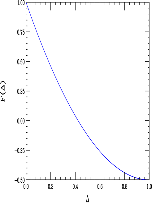
with being the locations of the left-handed lepton doublets of the first two generations. In the case where gauge fields are odd the last term can be dropped otherwise the two terms can be combined into a single term : , which means that the correction due to tower exchanges depends only upon the relative positions of the two lepton doublets. In this case we find that we can write as
| (6) |
with and shown in Fig.1. With the help of Ref. [9] one finds that can be obtained analytically: . Note that in the limit where the ’s are generation independent, so that and cases I and II yield identical results. It is very important to observe that, unlike the parameter introduced into the Rizzo and Wells[4] analysis, can have either sign and even vanishes when . In the case where the odd pieces are dropped we can still re-write into a form similar to the above with the replacement which remains a function of two variables. Scanning over the , however, we again find that the sum, i.e., is bounded to the region as was .
Given the shift in due to KK exchange it is straightforward to calculate the first order shifts in other electroweak observables due to which we imagine (due to the great success of the SM) to be rather small, i.e., of order or less. Thus we are free in our analysis below to drop terms in that are of more than linear order; this assumption is justified by our final results. We find that
| (7) |
where is the value of the effective weak mixing angle, ( boson mass) and is the decay width for in the SM after all of the SM QED, QCD and electroweak radiative corrections have been included. Here and are the third component of weak isospin and the electric charge of the fermion, , respectively. For , the widths are usually quoted through the ratios ; the shifts in these ratios are given by
| (8) |
where both sums in the last expression extend over all hadrons. These are the electroweak variables we will employ in our fit. Unlike in the case of Rizzo and Wells, we cannot make use of other observables, such as weak charge measured in atomic parity violation or data arising from deep inelastic neutrino scattering, since they necessarily involve five of the for the neutrino/electron and the and quarks.
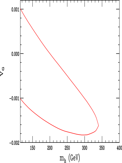
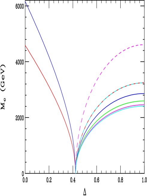
Using the latest precision electroweak data[12] as well as the updated estimate of [13] obtained from the new low energy data on [14] from the BES-II Collaboration, we find the CL allowed region in the -Higgs mass() plane shown in Fig.2 for Case I. (All electroweak radiative correction calculations are performed with ZFITTER6.23[15].) We recall that this same fit in the SM requires GeV at this level of confidence; here we see that the extra degree of freedom present in allows the SM Higgs mass to be as heavy as 350 GeV. Note that for GeV the CL plot requires . Since is known we can use these results to obtain a bound on as a function of for fixed values of which is also shown in Fig.2 for Case I. The first thing to note is that in the case where the ’s are family independent, i.e., the value of must be larger than about 4 TeV given the current lower bound on the Higgs mass GeV. (This same result applies also for Case II.) We see that as we vary both and the resulting bounds range from zero to over 6 TeV with typical values of order 2-5 TeV. A scan of the model parameters for Case II gives qualitatively very similar results. From this analysis it is clear that a bound of TeV is rather typical and we will use this value in our analysis below. To reach such KK resonance mass scales will either require CLIC[16] technology or a muon collider[17] either of which should have integrated luminosities in excess of 1 ab-1=1000 fb-1. Thus it is of particular importance what we can learn from data available below the first KK peak.
3 Localizing Fermions at Lepton Colliders
3.1 Bhabha Scattering
In order to localize the various SM fermions we must first determine the positions of the particles in the initial state, i.e., for an collider we must determine the values of and . (From now on we will drop the family index except where such labels are important and we will denote and .) This can best be done via Bhabha scattering for which the cross section is given by
| (9) | |||||
where and are the couplings of the electron(or muon) to the various gauge bosons, e.g., . Here we have employed the usual Mandelstam variables and have made use of the notation
| (10) |
with being the mass (width) of the gauge boson and where we have defined the polarization projectors [18],
| (11) |
with being the polarizations of the incoming electron and positron beam respectively.
It is instructive to conveniently bin the contributions to the above sum so they can be individually examined. First, we know that the pure SM terms are independent of the . Next, let us consider the sum of the contributions from a single gauge boson KK level due to a specific type of gauge boson, e.g., for fixed . In case I, summing over the even and odd fields yields an effective rescaling
| (12) |
For the first two coupling combinations, the resulting scale factor is just unity while in the last combination we obtain a factor of . This shows that the pure KK tower terms are either independent of the or will only depend upon the absolute value of the difference since cosine is an even function. In case II the corresponding rescaling factors are and thus showing the separate dependence on both and . The last set of terms are those due to interference between, e.g., the SM and for fixed , again summing over states. This set of terms scale similarly to the pure KK contribution except that they are not squared. Putting this all together demonstrates that for case I Bhabha scattering will only probe the quantity while for case II it will probe and independently.
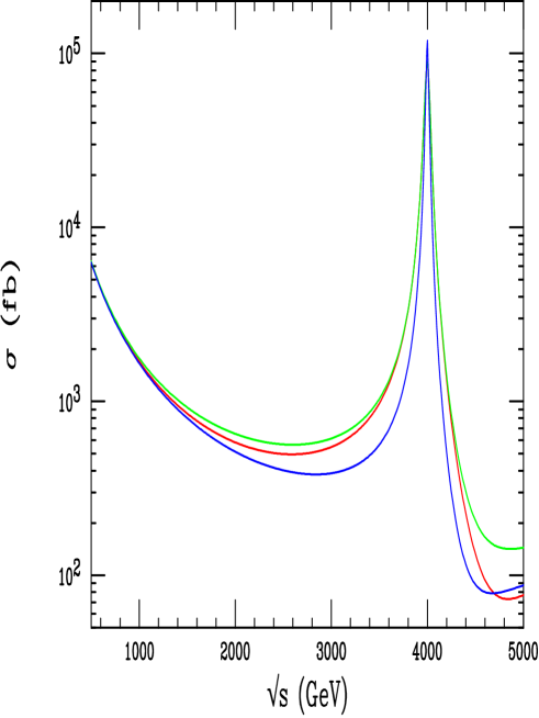
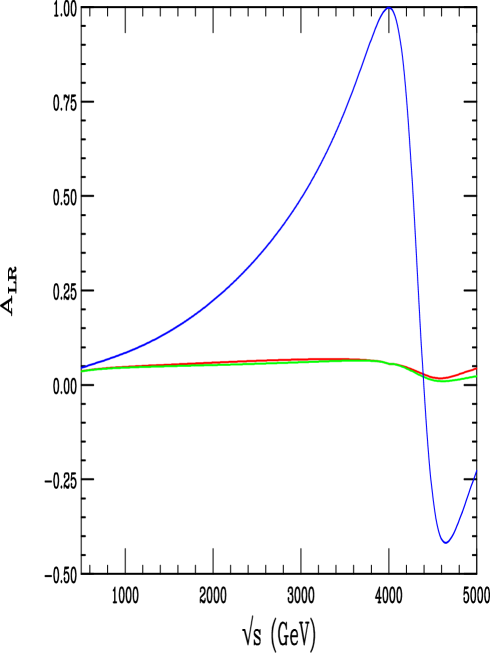
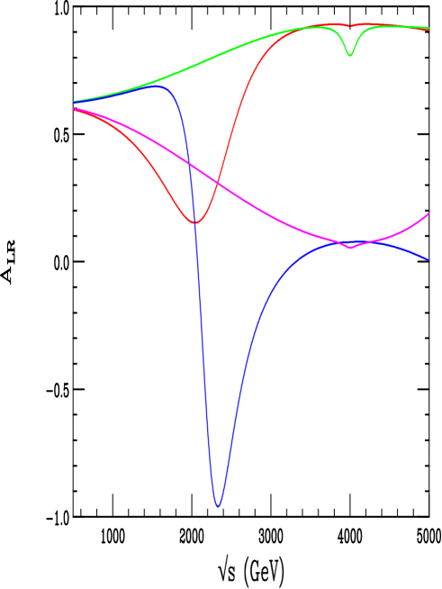
To get a feeling for these cross sections we show in Fig.3 the integrated cross section and the Left-Right Polarization asymmetry, as a function of energy assuming TeV for the common degenerate masses of and , for three different models. In all cases we assume an angular cut ; the stronger cut for positive is to remove a significant amount of the SM photon pole. In this plot and in the rest of the analysis below neither initial state radiation nor beamstrahlung corrections have been applied; for more realistic simulations these will need to be included but we know that these corrections will not change our results qualitatively. To generate the curves in the resonance region, family independence was assumed along with the specific values .
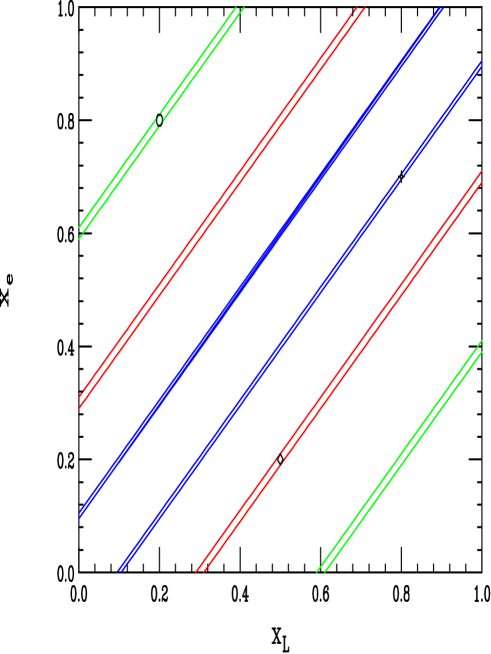
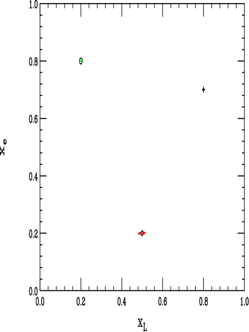
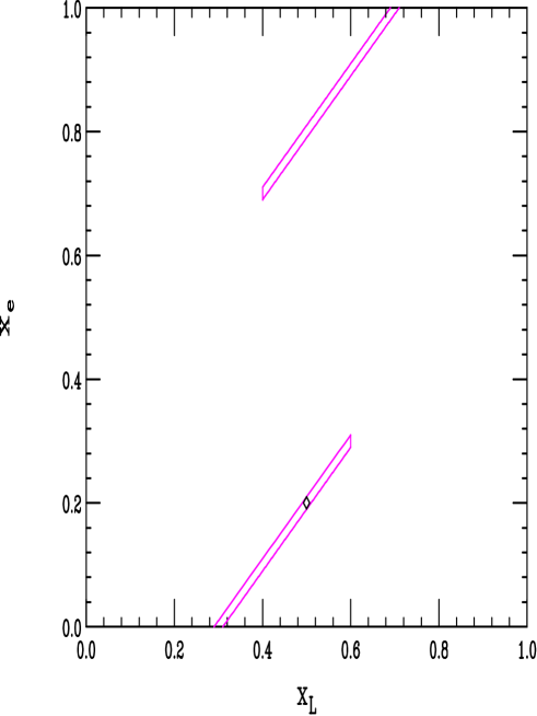
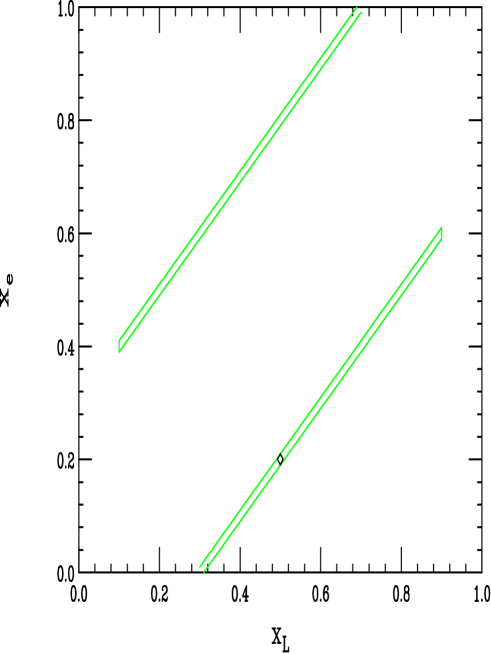
How well can we extract information from Bhabha scattering? Clearly at low energies below TeV neither the cross section nor appears to have any analyzing power. Once the 4 TeV pole is approached, say within a few widths, we become sensitive to the fact that we have assumed generation independence and the particular values above for all the other . Clearly the mass region near the pole should not be included in this fit. Thus we propose slicing up the region GeV into 25 points and accumulating 100 fb-1 of luminosity at each point, determining at each both and as well as the Forward-Backward asymmetry, , and the Polarized Forward-Backward asymmetry, . (This approach is certainly not optimized but will give us a flavor of what we may expect.) We now employ symmetrized cuts , assume a single beam polarization, , of , with an error of and we will also assume an error of on the integrated luminosity. For various input choices of we can ask what the extracted allowed region may be; as typical examples to cover the whole parameter space we will assume that = (0.2,0.8), (0.5,0.2), or (0.8,0.7). Fig.4 shows the results of performing this fit for case I while Fig.5 shows the corresponding results for case II. In case I, since we have already demonstrated that only the absolute value of the difference between and can be determined, we should not be surprised to see that that allowed regions take the form of pairs of stripe-like narrow bands. For example, when and , the resulting allowed regions should surround the lines and this is indeed what we find. The allowed regions in each of the examples lie between the narrowly separated pairs of lines; the typical separation of these two lines in the vertical direction is but varies somewhat from case to case by as much as a factor of two. This is the best that one can do for case I using data from Bhabha scattering alone. For case II the can be individually determined quite precisely without ambiguity for all three examples as shown in Fig.5. One sees that the size of the allowed regions are about the same or smaller than the the symbol marking the input values themselves.
3.2 Fermion Pair Production
To go further with our analysis we need turn our attention to the -channel fermion pair production process which has a cross section given by
| (13) | |||||
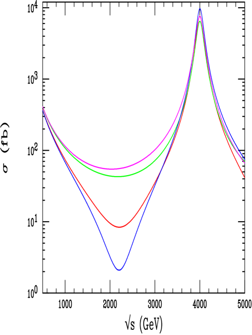
using the same notation as above. Fig.6 shows that, indeed, the cross section and are quite sensitive to variations in the in the same region employed in the case of the Bhabha scattering data fit.
By examining the various pieces that contribute to the cross section as above we can learn the structure of its sensitivity to the . If we concentrate on the pure KK contributions we obtain the effective rescalings
| (14) |
which for case I means that at least this part of the cross section depends only upon the absolute values of four distinct differences that one can form between the various . The SM-KK tower interference terms are found to scale exactly as above without squaring the factors on the right making this conclusion valid for almost the entire cross section. Note that unlike the case of Bhabha scattering, there are no terms in the cross section which are independent beyond those arising from the SM. For case II the same expressions as above are found to hold but with all the terms proportional to set to zero.
One might believe that since the cross section for case I now depends upon four absolute values of differences while Bhabha scattering provides a fifth absolute difference, it may be possible to uniquely determine all the ’s when the two sets of data are combined. Unfortunately, this is not the case as a simple example shows. Imagine the take on the particular set of values ; certainly if one adds or subtracts a common value, , to all of the the absolute values of the differences upon which the cross sections depend will be left invariant as long as none of the exceed unity or is less than zero as a result of this shift. This implies that the size and location of the CL allowed region on the projection for case I will critically depend, e.g., in the case of -quarks, on both and . An example of this is shown in Figs.7 and 8 where Bhabha scattering and data are combined in an effort to extract the four parameters , , and . (Here a b-tagging efficiency of has been used and QCD corrections have been included; we fit to the data taken at the same energy points with the same integrated luminosity as we have already done for the Bhabha analysis.)
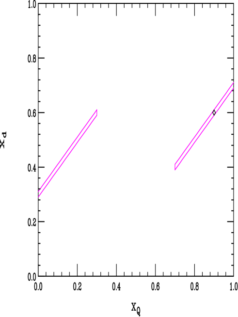
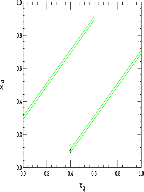
As we can see from these figures the inclusion of data does decrease the size of the stripe-shaped allowed range extracted for from Bhabha scattering but not by a very great amount. We also see that the locations of the allowed regions do depend on the assumed values of . We should be reminded that since these plots are 2-dimensional projections of the 4-dimensional fits, the various points in the allowed regions shown in Figs. 7 and 8 are highly correlated.
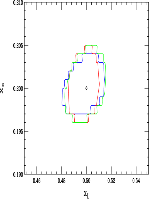
In case II there are no ambiguities in any of the couplings and, as in the case of Bhabha scattering, only a very small allowed region is found from the fit. The size of the allowed region on the plane is this case is found to be independent of the values of and not much different than that obtained from Bhabha scattering alone. All three examples are compared in Fig.9.
From this analysis it is clear that for case II precision measurements of the various fermion SM locations is relatively easy to achieve and is quite probably dominated by systematic uncertainties. For case I precision measurements of fermion locations may be possible as well although it would seem that fits to only one or two processes leads to bounded, striped-shape regions. Clearly as more and more final state fermion locations are probed the lengths and locations of these stipes will be reduced. It may be possible that if data on a sufficient number of final states can be collected the allowed striped-shaped regions will be cut down to a sufficient size so that a precise location determination is achievable. Such an analysis is, however, beyond the scope of the present paper so that we must for the moment be satisfied with our rather narrow striped allowed regions for the fermions’ locations.
3.3 On-Resonance Observables
In our earlier work[10] it was shown that once we determine that the spin of a resonance in lepton-pair collisions is one (from decay angular distributions) it will be straightforward to determine whether or not it is a KK state or a more typical provided beam polarization is available. This rests on the use of factorization tests, i.e., linear relationships between measurements of observables made atop the resonance. As is well-known, on a resonance the tree-level coupling factorization relationship is known to hold for any final state fermion . However, in the KK case, a single particle resonance is not what is produced. In case I(II) a coherent, resonating combination of 4(2) states is produced simultaneously so we expect relations such as the above to fail. (In earlier work[10] this was explicitly shown to happen for the rather simple case II so that it is rather obvious that it also happens for more complex case I. In this discussion we omit the possibility of any tiny mass splittings of order 1 GeV between the and states.) This can clearly be seen as follows: a short exercise shows that the above observables on resonance can be written as
| (15) |
where labels the final state fermion and we have defined the coupling combinations
| (16) |
with the individual widths of the contributing KK states. For case I, the sum extends over and while for case II only the states and are included. Note that as long as all of the are of comparable magnitude factorization relations of the type above are impossible to satisfy. Only in the limit where one of the dominates the sum (or, of course, when only one state is produced) will factorization be obtainable. Once factorization fails we then know that we are producing more than a simple single resonance.
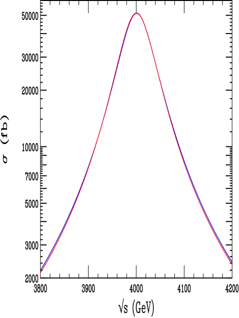
We note in passing that it is often asked whether it may also be possible to distinguish a single -like resonance from a KK state by the shape of the excitation spectrum. Such an analysis would need to include the effects of both the slight mass difference in the and states, initial state radiation, finite mass resolution, as well as the appropriate beamstrahlung spectrum corrections and has yet to be performed. Fig.10 shows what a comparison of a KK excitation and a single fitted Breit-Wigner(BW) may look like after ISR and beamstrahlung have been de-convoluted. Near the peak the BW is somewhat more narrow than the actual distribution and overestimates the cross sections in the tails. The actual KK distribution is also seen to be somewhat narrower above than below the resonance peak. Given these small differences it is clear that a detailed analysis must be performed to demonstrate whether or not a KK state can be distinguished from a single BW due to the importance of systematic uncertainties.
With the above discussion, we may ask what information can be obtained on the from resonance measurements; certainly statistics is not problem with more than events expected per ab-1. With these huge statistics it is clear that any such a determination of couplings will be systematics limited for either case I or case II. The simplest case to analyze, in the absence of any family symmetry and in analogy with Bhabha scattering, is the final state. In this case, the couplings in Eqs. (15) and (16) only depend upon the two unknowns ; however, the asymmetry observables also depend on the three(one) independent ratios of widths, , in case I(II). Thus for case I, there are not enough observables in this sector alone to fix all of the parameters while a unique solution seems to be obtainable in case II. For case I it is clear that one must combine the data from several flavor sectors in order to obtain a sufficient number of constraints to determine the relevant and from a rather large simultaneous fit. Such an analysis is beyond the scope of this paper. For case II, knowing , and the single width ratio , it would appear that we can proceed to all the other sectors and determine the corresponding without much difficulty. However in the case of electrons there are actually only two independent asymmetries since . Thus, as in case I, data from other final states will need to be included and a large simultaneous fit performed. It is clear from this discussion that it will be somewhat easier to isolate the positions of the various SM fermions in the extra dimensions by using off-resonance measurements than via on-peak data.
4 Summary and Conclusions
In this paper we have investigated the capability of future lepton colliders to probe the locations of the SM fermions when they are ‘stuck’ at specific points in extra dimensions as suggested by the Arkani-Hamed-Schmaltz model. There were several major steps necessary to perform this analysis which we now summarize.
-
•
We consider two classes of models: I and II; they differ by whether or not the odd components of the gauge KK towers are allowed to propagate and couple to the SM fermions. These two classes of models are identical when the fermions live at the fixed points put differ significantly if the fermions can live at arbitrary locations.
-
•
In order to investigate the fermion locations at an accelerator the first requirement is to determine the scale of the the compactification which determines the mass of the KK gauge boson spectrum. Direct searches for such states at the Tevatron only provide limits[10] on the TeV range while those from indirect searches, i.e., the use of precision electroweak data, can provide limits in the several TeV range. For the case at hand, allowing for the left-handed electron and to occupy different locations within the thick wall, we found KK mass constraints that are fairly sensitive to the separation of these two fields as well as the SM Higgs mass. Scanning over the parameter space a typical bound we obtained by this procedure is TeV. In some cases it may be possible to obtain a higher average bound by considering various FCNC processes but these are much more model dependent. Clearly, to reach and probe the TeV scale with sufficient statistics will require CLIC or a Muon Collider with very high integrated luminosities .
-
•
Since this center of mass energy is quite high it is important that we first ascertain what can be learned from data taken below the resonance. In this energy range, for any given process such as , the cross section and various asymmetries depend only upon the locations of these specific fermions, i.e., and . The simplest process to consider is thus Bhabha scattering. Dividing the mass range up into bins of equal integrated luminosity and making use of the cross section and asymmetry observables we were able to obtain the allowed regions for the locations of which differed significantly for cases I and II. In case I we found, consistent with theoretical expectations, that only the quantity could be precisely determined, with the allowed parameter space thus appearing as striped-shaped regions in the plane, whereas in case II both can be well-determined separately. Adding information from another process, such as , led to a four parameter fit; for case I the size and locations of the allowed regions in location space were shown to be rather sensitive to the assumed values of the input parameters. On the otherhand, in case II the fermion location sensitivity was observed not to be sensitive to the choice of input. If case II holds, it is clear that from a generalization of our procedure to other fermion final states that locating the SM fermions will be rather straightforward using data obtained below the first KK pole. For case I such a situation is more problematic since the allowed regions, projected in two dimensions, are stripe-shaped. It may be, however, that if enough final states are accessible, a large simultaneous fit can lead to rather small allowed regions for the various fermion locations.
-
•
We demonstrated that on-resonance measurements will be much harder to use in determining fermion locations. The reason for this is that for any particular fermion decay mode, the locations of all the SM fermions are involved in determining the value of the associated observables. Fortunately, we demonstrated that the these additional dependencies can be isolated into a only one(for case II) or three(for case I) additional unknowns when conducting the appropriate fits. Even with this simplification, however, we argued that large simultaneous fits involving many observables will be necessary to extract location information for either case I or II in order to obtain a sufficient number of independent quantities to fit the rather large number of unknowns. Given the huge on-resonance statistics, the errors in such fits will certainly be systematics dominated. In addition, we speculated on the possibility of distinguishing a KK resonance from a single Breit-Wigner through its’ shape; such an analysis will require a detailed study including initial state radiation, beamstrahlung and finite energy resolution effects and is beyond the scope of this paper.
From our analysis it is clear that future lepton colliders will provide a means to map out the positions of SM fermions if they are localized in extra dimensions.
Acknowledgements
The author would like to thank N. Arkani-Hamed, Y. Grossman and M. Schmaltz for discussions on localized fermion models during the early stages of this work. The author would also like to thank H. Davoudiasl and J.L. Hewett for general discussions on models with extra dimensions.
References
- [1] See, for example, I. Antoniadis, Phys. Lett. B246, 377 (1990); I. Antoniadis, C. Munoz and M. Quiros, Nucl. Phys. B397, 515 (1993); I. Antoniadis and K. Benalki, Phys. Lett. B326, 69 (1994)and Int. J. Mod. Phys. A15, 4237 (2000); I. Antoniadis, K. Benalki and M. Quiros, Phys. Lett. B331, 313 (1994); K. Benalki, Phys. Lett. B386, 106 (1996); E. Accomando, I. Antoniadis and K. Benalki, Nucl. Phys. B579, 3 (2000).
- [2] H. Davoudiasl, J.L. Hewett and T.G. Rizzo, Phys. Lett. B473, 43 (2000); A. Pomarol, Phys. Lett. B486, 153 (2000).
- [3] L. Randall and R. Sundrum, Phys. Rev. Lett. 83, 3370 (1999).
- [4] See, for example, T.G. Rizzo and J.D. Wells, Phys. Rev. D61, 016007 (2000); P. Nath and M. Yamaguchi, Phys. Rev. D60, 116006 (1999); M. Masip and A. Pomarol, Phys. Rev. D60, 096005 (1999); W.J. Marciano, Phys. Rev. D60, 093006 (1999); L. Hall and C. Kolda, Phys. Lett. B459, 213 (1999); R. Casalbuoni, S. DeCurtis and D. Dominici, Phys. Lett. B460, 135 (1999); R. Casalbuoni, S. DeCurtis, D. Dominici and R. Gatto, Phys. Lett. B462, 48 (1999); A. Strumia, Phys. Lett. B466, 107 (1999); F. Cornet, M. Relano and J. Rico, Phys. Rev. D61, 037701 (2000); C.D. Carone, Phys. Rev. D61, 015008 (2000); A. Delgado, A. Pomarol and M. Quiros, J. High En. Phys. 0001, 030 (2000.)
- [5] T. Appelquist, H.-C. Cheng and B.A. Dobrescu, hep-ph/0012100. See also R. Barbieri, L.J. Hall and Y. Nomura, hep-ph/0011311.
- [6] H. Davoudiasl, J. L. Hewett and T. G. Rizzo, hep-ph/0006041 and Phys. Rev. Lett. 84, 2080 (2000).
- [7] N. Arkani-Hamed and M. Schmaltz, Phys. Rev. D61, 033005 (2000).
- [8] E.A. Mirabelli and M. Schmaltz, Phys. Rev. D61, 113001 (2000); G.C. Branco, A. De Gouvea and M.N. Rebolo, hep-ph/0012289.
- [9] N. Arkani-Hamed, Y. Grossman and M. Schmaltz, Phys. Rev. D61, 115004 (2000).
- [10] T.G. Rizzo, Phys. Rev. D61, 055005 (2000).
- [11] There are huge number of references; see for example V.A. Rubakov and M.E. Shaposhnikov, Phys. Lett. B125, 136 (1983); G. Dvali and M. Shifman, Phys. Lett. B396, 64 (1997); M. Bando, T. Kugo, T. Noguchi and K. Yoshioka, Phys. Rev. Lett. 83, 3601 (1999); J. Hisano and N. Okada, Phys. Rev. D61, 106003 (2000); H. Georgi, A. Grant and G. Hailu, hep-ph/0007350; A. DeRujula, A. Donini, M.B. Gavela and S. Rigolin, Phys. Lett. B482, 195 (2000).
- [12] B. Pietrzyk, talk given at the XXXth International Conference on High Energy Physics, ICHEP2000, Osaka, Japan, 27 July-2 August, 2000.
- [13] For an updated calculation, see A.D. Martin, J. Outhwaite and M.G. Ryskin, hep-ph/0012231.
- [14] Z. Zhao, BES-II Collaboration, talk given at the XXXth International Conference on High Energy Physics, ICHEP2000, Osaka, Japan, 27 July-2 August, 2000.
- [15] D. Bardin, hep-ph/9412201.
- [16] I. Wilson, talk given at The 2000 International Workshop on Linear Colliders, Fermilab, Batavia, IL 24-28 October, 2000. See also J.-P. Delahaye et al., The CLIC Study of a Multi-TeV Linear Collider, CERN/PS 99-005.
- [17] B.J. King, talk given at Colliders and Collider Physics at the Highest Energies, Montauk, NY, 27 September-1 October, 1999.
- [18] See for example, F. Cuypers, hep-ph/9611336, in New Directions for High High Energy Physics, Proceedings of the 1996 DPF/DPB Summer Study on High Energy Physics, eds. D.G Cassel, L.T. Gennari and R.H. Siemann, Snowmass, CO 1996.