Nonlinear evolution and saturation
for heavy nuclei in DIS.

Abstract

The nonlinear evolution equation for the scattering amplitude of colour dipole off the heavy nucleus is solved in the double logarithmic approximation. It is found that if the initial parton density in a nucleus is smaller then some critical value, then the scattering amplitude is a function of one scaling variable inside the saturation region, whereas if it is greater then the critical value, then the scaling behaviour breaks down. Dependence of the saturation scale on the number of nucleons is discussed as well.

TAUP-2664-2001

1 Introduction

In the two previous publications[1, 2] we solved the nonlinear evolution equation for high parton density QCD[3, 4, 5, 6, 7, 8, 9, 10, 11, 12, 13] in the double logarithmic approximation and discussed its properties. We showed that at high energies there is a momentum scale $Q^{2}_{s}(y,A)$, where $y=\ln(1/x_{B})$ is a rapidity, at which the parton evolution can no longer be described by linear evolution equation. This so-called saturation scale, has the following dependence on the energy and the number of nucleons (for DIS on a nucleus): $Q^{2}_{s}(y,A)\sim A^{\frac{2}{3}}e^{4\bar{\alpha}_{s}y}$, which holds in the double logarithmic approximation. In Ref. [1, 2] we derived this result assuming that initial parton density is not very large.

The $A$ dependence of the saturation scale can be also obtained using simple qualitative arguments. Indeed, as one increases energy and/or decreases virtuality of the photon, the density of partons inside the nucleus grows until they begin to overlap in the transverse plane. The scale at which this occurs is proportional to $Q^{2}_{s}(y,A)$ and can be estimated from the equation

$$\frac{A\pi\vec{x}^{2}x_{B}G(x_{B},Q^{2}_{s})}{\pi R_{A}^{2}}=1\quad,$$ (1)

where $\vec{x}$ is a colour dipole, $x_{B}G(x_{B},Q^{2}_{s})$ is the proton structure function and $R_{A}$ is the nucleus radius. Since in the kinematical region intermediate between the linear and the saturation ones, the anomalous dimension of the gluon structure function $\gamma\approx\frac{1}{2}$[9, 10, 14] and $R_{A}\sim A^{\frac{1}{3}}$, one obtains that $Q_{s}^{2}\sim A^{\frac{2}{3}}$.

It was shown in Ref. [7] that the initial condition for the nonlinear evolution equation is given by the Glauber–Mueller formula[15]

$$N(\vec{x},y=y_{0})=1-e^{-\frac{\alpha_{s}\pi^{2}}{2N_{c}}\vec{x}^{2}\;x_{B}G(x_{B},4/\vec{x}^{2})\;S(b_{t})}\quad,$$ (2)

where $S(b_{t})$ is a nucleus profile function and $b_{t}$ is an impact parameter. If $b_{t}<R_{A}$, $S=\frac{3A}{2\pi R_{A}^{2}}$ (Woods-Saxon parameterization[16]), which implies that initially the saturation scale $Q^{2}_{s}$ is proportional to $A^{\frac{1}{3}}$. So, the question arises how it becomes proportional to $A^{\frac{2}{3}}$ at large energy. There is an opinion that the only dimensionful scale in the high energy DIS is the scale set by initial condition. It would imply that the $A$ dependence of the saturation scale set by initial condition Eq. (2) remains the same during the evolution since the evolution equation is conformally invariant. This however is not the case since there is another dimensionful scale which comes through the Glauber–Mueller initial condition Eq. (2). Indeed, in our estimations we neglected for simplicity the logarithmic dependence of the gluon structure function $x_{B}G$ of the nucleon on $\vec{x}^{2}$. However, this dependence on $\ln(\vec{x}^{2}\Lambda^{2})$ introduces the second dimensionful parameter $\Lambda$ which is the soft QCD scale. In other words, the relevant scale for the evolution in the nucleon is $\Lambda^{2}$ while that in nucleus is $A/R_{A}^{2}$. The later one as we see is set by the nucleus size. The former one means that evolution can occur in a nucleon as well as in nucleus.

The goal of our paper is to derive the saturation scale in the semiclassical double logarithmic approximation and discuss its dependence on $A$ and energy. We consider the nonlinear evolution equation derived by Yu. Kovchegov[6, 7] in the framework of Mueller’s dipole model[17] and solve it using semiclassical methods (on characteristics) in the double logarithmic approximation. We show that there exist a certain characteristic, which divides the whole kinematical region into two patches: one in which the evolution is linear and another in which the parton density saturates. The remarkable property of this characteristic is that the dipole number remains fixed along it. This characteristic coincides with the critical line in the double logarithmic approximation[3, 9, 18]. Recall[1] that the critical line is defined by $r=\left(\ln Q^{2}_{s}(y,A)/4\Lambda^{2}\right)$, where $r=\left(\ln Q^{2}/4\Lambda^{2}\right)$.

In this paper the same strategy as in Ref. [1] will be employed to solve the evolution equation. Namely, we will solve it in the two kinematical regions where: (i) $\gamma$ is small ($Q^{2}>Q_{s}^{2}$, $Q^{2}\gg\Lambda^{2}$) and (ii) $\gamma$ is close to unity ($Q^{2}\ll Q_{s}^{2}$). Then the two solutions will be matched in the intermediate region. It turns out that the solution inside the saturation region depends strongly on the initial parton density inside nucleus. In the Fig. 1 we show two possible situations. If the nucleus is light, then the Glauber initial condition is out of the saturation region. We argued in Ref. [1] (and will re-derive in this paper again) that the parton density is constant along the critical line. This condition sets the initial condition for the solution inside the saturation region. As the result, this solution is a function of only one variable. This case was studied in Ref. [1, 2] and will be derived again using another approach in Sec. 3.

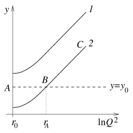
Figure 1: The kinematical regions relevant in high parton density QCD. The initial condition Eq. (2) for the nonlinear evolution equation Eq. (3) is set on the line $y=y_{0}$ (dashed line). Solid curves 1,2 are the critical lines $r=\left(\ln Q_{s}^{2}/4\Lambda^{2}\right)$ for different nuclei: $A_{1}<A_{2}$. Initial conditions for the solution to the left of the critical line are set along line 1 for nucleus $A_{1}$ or along line $ABC$ for nucleus $A_{2}$.

On the other hand, if the initial parton density is large (because the nucleus is very heavy), then one has to match solution inside the saturation region to both the condition on the critical line $BC$ ($y>y_{0}$), and Glauber initial condition $AB$ ($y=y_{0}$), see Fig. 1. This cannot be done with the scaling solution, so the scaling solution breaks down for very heavy nuclei. We will investigate both cases in Sec. 3.

As usually we use the nonlinear evolution equation derived in Ref. [7] in the framework of the dipole model[17]. Since colour dipoles diagonalize the scattering matrix at high energies[19, 17] we consider this approach as the most clear from the physical point of view. The evolution equation for the dipole-nucleus forward scattering amplitude $\tilde{N}(k,y)$ in the momentum representation reads

$$\frac{\partial\tilde{N}(k,y)}{\partial y}=\bar{\alpha}_{s}\hat{\chi}\left(\hat{\gamma}(k)\right)\tilde{N}(k,y)-\bar{\alpha}_{s}\tilde{N}^{2}(k,y)\quad,$$ (3)

where $\hat{\chi}\left(\hat{\gamma}(k)\right)$ is an operator such that

$$\hat{\gamma}(k)=1+\frac{\partial}{\partial\ln k^{2}}$$ (4)

is an operator corresponding to the anomalous dimension of the gluon structure function and the operator $\hat{\chi}$ corresponds to the following function

$$\chi\left(\gamma\right)=2\psi\left(1\right)-\psi\left(1-\gamma\right)-\psi\left(\gamma\right)$$ (5)

which is an eigenvalue of the the BFKL equation. Eq. (3) is derived assuming that the typical transverse extent of the dipole amplitude is much smaller then the size of the target and the typical impact parameter $x\ll R_{A},b_{t}$.

The amplitude in the dipole configuration space is found by employing the Fourier transform

$$N(x,y) = \vec{x}^{2}\int_{0}^{\infty}dk\,kJ_{0}(kx)\tilde{N}(k,y)$$ (6)

$$\tilde{N}(k,y) = \int_{0}^{\infty}\frac{dx}{x}J_{0}(kx)N(x,y)\quad.$$ (7)

Initial condition for this equation in the dipole configuration space reads (see Eq. (2))

$$N(x,y=y_{0})=1-e^{-\exp(-r+r_{A})}\quad,$$ (8)

where $r_{A}=\ln\left(\frac{\bar{\alpha}_{s}\pi^{2}x_{B}G(x_{B},4/\vec{x}^{2})S(0)}{2N_{c}\Lambda^{2}}\right)$ and $r=\ln(Q^{2}/4\Lambda^{2})$ for $Q^{2}>Q_{s}^{2}$. In the double logarithmic approximation one can neglect the logarithmic dependence of $x_{B}G(x_{B},4/\vec{x}^{2})$ as well as $\alpha_{s}$ on the dipole size, and in addition $Q^{2}\approx 4/\vec{x}^{2}$.

Eq. (8) can be Fourier transformed to the momentum space where it reads

$$\tilde{N}(k,y)=\frac{1}{2}\Gamma_{0}\left(\frac{k^{2}e^{-r_{A}}}{4\Lambda^{2}}\right)\quad,$$ (9)

where $\Gamma_{0}$ is incomplete gamma function of zeroth order.

2 Solution at $Q^{2}>Q_{s}^{2}(x_{B})$.

Function $\chi(\gamma)$ is singular at its end-points $\gamma=0,1$. The first one corresponds to the kinematical region $Q^{2}>Q_{s}^{2}(y)$, whereas the second to the kinematical region $Q^{2}\ll Q_{s}^{2}(y)$. Expansion of $\chi(\gamma)$ near its end-points and taking the leading contribution corresponds to the double logarithmic approximation, i.e. to the summation of $\alpha_{s}^{n}\ln^{n}(Q^{2}/\Lambda)\ln^{n}(1/x_{B})$ terms to the right of the critical line, and to the summation of $\alpha_{s}^{n}\ln^{n}(Q_{s}^{2}/Q^{2})\ln^{n}(1/x_{B})$ terms to the left of it.

In the right vicinity of the $\gamma=0$ one obtains using Eq. (4)

$$\chi=\frac{1}{\gamma}=\frac{1}{1+\partial_{r}}\quad.$$ (10)

Eq. (3) in this approximation reads

$$\tilde{N}_{y}(r,y)=\bar{\alpha}_{s}(1+\partial_{r})^{-1}\tilde{N}(r,y)-\tilde{N}(r,y)^{2}\quad.$$ (11)

In this paper we will always denote the partial derivatives by subscripts. Note, that the following equation

$$(1+\partial_{r})\cdot\frac{1}{k^{2}}\int_{\Lambda^{2}}^{k^{2}}\;dk^{{}^{\prime}2}\;\tilde{N}(k^{\prime},y)=\tilde{N}(k,y)$$ (12)

identifies the operator inverse to $1+\partial_{r}$. Introducing the new function $G$ by

$$G(k,y)=\int_{\Lambda^{2}}^{k^{2}}\;dk^{{}^{\prime}2}\;\tilde{N}(k^{\prime},y)\quad,$$ (13)

one gets for it the following equation:

$$G_{ry}(r,y)=\bar{\alpha}_{s}G(r,y)-e^{-r}(G_{r}(r,y))^{2}\frac{1}{\Lambda^{2}}\quad.$$ (14)

The advantage of introducing the function $G$ is that we got the nonlinear evolution equation in which the nonlinear term has the simplest form.

Having in mind the success of the semiclassical approach to solution of the DGLAP evolution equation at low $x_{B}$, we look for the solution to the Eq. (14) in the form

$$G(r,y)=e^{S(r,y)}\Lambda^{2}\quad,$$ (15)

where the function $S$ is supposed to be such that $|S_{r}S_{y}|\gg|S_{ry}|$. Equation for $S(r,y)$ is

$$S_{r}(r,y)S_{y}(r,y)=\bar{\alpha}_{s}-e^{-r+S(r,y)}S_{r}^{2}(r,y)\quad.$$ (16)

This is a partial differential equation of the first order and can be solved by characteristics method. Denote $S_{r}=f$ and $S_{y}=\omega$. Then, the characteristics of the Eq. (16) can be found by solving the system of ordinary differential equations[20]

$$\frac{dr}{dt} = \omega+2fe^{-r+S}\quad,$$ (17)

$$\frac{dy}{dt} = f\quad,$$ (18)

$$\frac{dS}{dt} = 2f\omega+2f^{2}e^{-r+S}\quad,$$ (19)

$$\frac{df}{dt} = e^{-r+S}f^{2}(1-f)\quad,$$ (20)

$$\frac{d\omega}{dt} = -\omega e^{-r+S}f^{2}\quad,$$ (21)

where $t$ is the parameter along the characteristic. Using Eq. (16) in Eq. (19) one obtains

$$S=2\bar{\alpha}_{s}t+S_{0}\quad.$$ (22)

By subscript $0$ we distinguish the integration constants. It follows from Eq. (20) and Eq. (21) that

$$f-1=\frac{f_{0}-1}{\omega_{0}}\;\omega\equiv C\omega\quad.$$ (23)

Substituting Eq. (22) and Eq. (23) into Eq. (21) results in equation

$$\frac{d\omega}{dt}=(C\omega^{2}+\omega-\bar{\alpha}_{s})\omega=C\omega(\omega-\omega_{+})(\omega-\omega_{-})\quad,$$ (24)

where

$$\omega_{\mp}=\frac{-1\pm\sqrt{1+4C\bar{\alpha}_{s}}}{2C}\quad.$$ (25)

Consider some characteristic at large values of $r$ (at $t\rightarrow\infty$). In that region nonlinear term is small and Eq. (21) implies $\omega=\omega_{0}=\mathrm{const.}$ Moreover, $f_{0}$ is small and thus $\omega_{0}=\bar{\alpha}_{s}/f_{0}$ is large. It is straightforward to calculate $\omega_{+}$ and $\omega_{-}$ neglecting nonlinear terms

$$\omega_{+}=\omega_{0}\quad\mathrm{and}\quad\omega_{-}=\frac{\bar{\alpha}_{s}\omega_{0}}{\omega_{0}-\bar{\alpha}_{s}}\quad.$$ (26)

This shows that in the kinematical region of large $r$, where nonlinear term is small, solution of the system Eqs. (17-21) can be obtained by setting $\omega=\omega_{0}=\omega_{+}$ which yields us with the usual double logarithmic approximation to the DGLAP and BFKL equations.

As $t$ decreases $\omega$ will no longer be equal to $\omega_{0}$. Corrections stem from the nonlinear term (but $\omega_{0}=\omega_{+}$ still holds as it gives correct asymptotic behaviour of solution). Let us address the question of what happens if the deviation from the linear behaviour is small (this is equivalent to checking the stability of the linear solution). In other words, assume that $\omega=\omega_{0}+\delta\omega$ where $\delta\omega\ll\omega_{0}$. Inserting this into the Eq. (24) and integrating gives

$$\omega(t)=\omega_{0}\left(1+\beta e^{-(\omega_{0}-2\bar{\alpha}_{s})t}\right)\quad,$$ (27)

where $\beta$ is the integration constant, and by Eq. (23)

$$f(t)=\frac{\bar{\alpha}_{s}}{\omega_{0}}\left(1-\frac{\omega_{0}-\bar{\alpha}_{s}}{\bar{\alpha}_{s}}\beta e^{-(\omega_{0}-2\bar{\alpha}_{s})t}\right)\quad.$$ (28)

Finally, using Eq. (16),Eq. (27) and Eq. (28) in Eq. (17) and Eq. (18), the solution to the system Eqs. (17-21) at large $t$ reads

$$r-r_{0} = \omega_{0}t-\frac{2\omega_{0}-3\bar{\alpha}_{s}}{(\omega_{0}-2\bar{\alpha}_{s})\bar{\alpha}_{s}}\beta\left(e^{-(\omega_{0}-2\bar{\alpha}_{s})t}-1\right)\quad,$$ (29)

$$y-y_{0} = \frac{\bar{\alpha}_{s}}{\omega_{0}}t+\frac{\omega-\bar{\alpha}_{s}}{\omega_{0}(\omega_{0}-2\bar{\alpha}_{s})}\beta\left(e^{-(\omega_{0}-2\bar{\alpha}_{s})t}-1\right)\quad.$$ (30)

It is readily seen that if $\omega_{0}>2\bar{\alpha}_{s}$ the solution for characteristic is stable, which means that all nonlinear effects which are introduced through the (Glauber) initial condition die out exponentially as $t$ increases. By contrast, at $\omega_{0}<2\bar{\alpha}_{s}$ the solution is not stable.

This discussion reveals a remarkable property of nonlinear evolution equation: there exist such characteristic, that divides the whole kinematical region into two patches[1]. One in which all nonlinear effects are negligible, another in which saturation occurs. This line is given by condition $\omega_{0}=2\bar{\alpha}_{s}$. Using Eq. (29) and Eq. (30) we get the familiar equation for the critical line[1].

$$r-r_{0}=4\bar{\alpha}_{s}(y-y_{0})\quad.$$ (31)

In the next sections we will denote this line as $r_{s}(y)$ or $y_{s}(r)$.

Excluding $\omega_{0}$ and $t$ (at $r\rightarrow\infty$) from Eq. (29), Eq. (30) and Eq. (22) we arrive at the general solution of Eq. (16) in this limit:

$$S(r,y)=2\sqrt{\bar{\alpha}_{s}(r-r_{0})(y-y_{0})}+S_{0}\quad.$$ (32)

On the critical line $S|_{s}=r-r_{0}+S_{0}$ (we denote by symbol $|_{s}$ all quantities calculated on the critical line). Therefore, by Eq. (13) and Eq. (15)

$$\tilde{N}(k,y)|_{s}=\frac{1}{k^{2}}G_{r}(k,y)|_{s}=e^{S_{0}-r_{0}}=\mathrm{const.}$$ (33)

The dipole scattering amplitude is constant on the critical line. The value of this constant is given by Eq. (9):

$$\tilde{N}(y=y_{0},r=r_{A})=\frac{1}{2}\Gamma_{0}(1)\approx 0.1\quad,$$ (34)

in accord with our expectations that the critical line is the boundary of the linear region.

3 Solution at $Q^{2}<Q_{s}^{2}(x_{B})$.

In this section we solve the nonlinear evolution equation inside the saturation region. To this end expand $\chi$ in the left vicinity of the $\gamma=1$ using Eq. (5) and Eq. (4)

$$\chi=\frac{1}{1-\gamma}=-\frac{1}{\partial_{r}}\quad.$$ (35)

This results in the following equation (see Eq. (3))

$$-\tilde{N}_{y\>r}(r,y)=\bar{\alpha}_{s}\tilde{N}(r,y)\left(1+2\tilde{N}_{r}(r,y)\right)\quad.$$ (36)

Following Ref. [1] we introduce the auxiliary function $\varphi$ by

$$\tilde{N}(r,y)=\frac{1}{2}\int_{r}\;dr^{\prime}\;\left(1-e^{-\varphi(r^{\prime},y)}\right)\quad.$$ (37)

Note, that $r=\ln(Q^{2}/Q_{s}^{2})<0$ is defined with respect to the $Q_{s}^{2}$ which is the largest scale in this kinematical region. For the function $\varphi$ Eq. (36) takes especially simple form

$$\varphi_{yr}=-\bar{\alpha}_{s}\left(1-e^{-\varphi(r,y)}\right)\quad.$$ (38)

The idea of the solution is to split this equation into two and then to find such solution of one of the equations that satisfy the other as well. We are looking for the solution in the form $\varphi=\varphi(e^{\mathcal{S}})$, where $\mathcal{S}$ is assumed to be semiclassical, i.e. $|\mathcal{S}_{ry}|\ll|\mathcal{S}_{r}\mathcal{S}_{y}|$. In other words the function $\varphi$ is a quickly varying function of a slowly varying one $\mathcal{S}$. The form of splitting is inspired by the solution of the previous section. Namely, we restrict solutions of Eq. (38) by the requirement that

$$\mathcal{S}_{r}(r,y)\mathcal{S}_{y}(r,y)=-\mathcal{C}=\mathrm{const}.$$ (39)

In other words we assume that $e^{\mathcal{S}}$ satisfies the linearized equation (ı.e.  $\varphi\rightarrow 0$).

In the semiclassical approximation defined above, Eq. (38) can be rewritten as

$$\frac{d^{2}\varphi(\mathcal{S})}{d\mathcal{S}^{2}}=\frac{\bar{\alpha}_{s}}{\mathcal{C}}\left(1-e^{-\varphi(\mathcal{S})}\right)\quad.$$ (40)

To solve this equation we interchange the independent $\mathcal{S}$ and dependent $\varphi$ variables[1]. Denote

$$\zeta(\varphi)=\frac{d\varphi}{d\mathcal{S}}\quad.$$ (41)

Then, Eq. (40) reads

$$\frac{d\zeta(\varphi)}{d\varphi}\zeta(\varphi)=\frac{\bar{\alpha}_{s}}{\mathcal{C}}\left(1-e^{-\varphi(\mathcal{S})}\right)\quad,$$ (42)

and can be easily integrated for $\zeta$ and then for $\varphi$. the final result is

$$\mathcal{S}=\int^{\varphi(\mathcal{S})}\;\frac{d\varphi^{\prime}}{\sqrt{\frac{2\bar{\alpha}_{s}}{\mathcal{C}}(\varphi^{\prime}+e^{-\varphi^{\prime}})+\frac{\zeta_{0}^{2}}{2}}}+\mathrm{const.}$$ (43)

Now we turn to Eq. (39). It is merely the DGLAP equation in the double logarithmic semiclassical approximation. Applying the method of characteristics one arrives at the following system of equations

$$r(t,\tau) = \omega^{\prime}_{0}(\tau)\,t+r^{\prime}_{0}(\tau)\quad,\quad y(t,\tau)=f^{\prime}_{0}(\tau)\,t+y_{0}(\tau)\quad,\quad\mathcal{S}(t,\tau)=-2\,t\,\mathcal{C}+\mathcal{S}_{0}(\tau)\quad,$$

$$f^{\prime}(t,\tau) = f_{0}^{\prime}(\tau)=\mathrm{const}.\quad,\quad\omega^{\prime}(t,\tau)=\omega_{0}^{\prime}(\tau)=\mathrm{const}.$$

where we introduced the prime notation to distinguish variables of this sections from those in the previous one. $\tau$ parameterizes the initial condition which we specify below. By analogy with Eq. (32), Eq. (LABEL:SS1) give the general solution

$$\mathcal{S}(r,y)=2\sqrt{\mathcal{C}}\sqrt{-(r-r_{0}^{\prime})(y-y_{0})}+\mathcal{S}_{0}\quad.$$ (45)

Let us now specify the initial conditions for Eq. (38). They depend on the initial parton density inside a nucleus. If the initial density is small (curve 1 in the Fig. 1) then the results of Sec. 2 imply that

$$\varphi(y,r)|_{s}=\mathrm{const.}\quad$$ (46)

The initial condition is different in the case of large initial parton density (curve 2). In this region the initial condition reads:

$$\varphi(y,r)|_{s} = \mathrm{const.}\quad,\hskip 79.6678pt\mathrm{if}\quad y_{0}<y=y_{s}(r)\quad,$$ (47)

$$\varphi(y,r) = -\ln\left(1-e^{-\exp(r-r_{A})}\right)\quad,\quad\mathrm{if}\quad y=y_{0}\quad.$$ (48)

Eq. (48) follows from its definition Eq. (37) and Eq. (9).

Generally, to satisfy initial conditions one has to find such a surface among those given by the solution Eq. (LABEL:SS1) which paths through the line specified by Eq. (46) or Eq. (47) and Eq. (48). To do this one should parameterize the initial condition using parameter $\tau$. Then calculate $f_{0}^{\prime}(\tau)$ and $\omega_{0}^{\prime}(\tau)$ using the following equations[20]:

$$\frac{d\mathcal{S}_{0}}{d\tau}=f_{0}^{\prime}\;\frac{dr_{0}^{\prime}}{d\tau}+\omega_{0}^{\prime}\;\frac{dy_{0}^{\prime}}{d\tau}\quad,$$ (49)

and

$$f_{0}^{\prime}\;\omega_{0}^{\prime}=-\mathcal{C}\quad.$$ (50)

The desired solution of the Cauchy problem $\mathcal{S}(y,r)$ is then obtained by excluding $t$ and $\tau$ from Eq. (LABEL:SS1).

Eq. (49) and Eq. (50) can be easily solved numerically, but to give a transparent analytic treatment we notice that the nonlinear corrections in the kinematical region $Q^{2}<Q^{2}_{s}$ are so large that $e^{-\varphi}\ll 1$. Indeed, by Eq. (47) and Eq. (48), the value of $\varphi$ on the critical line $r=r_{s}(y)$ is

$$\varphi_{0}=-\ln\left(1-e^{-1}\right)\approx 0.5\quad,$$ (51)

which follows from the requirement that the point $(r_{A},y_{0})$ lies on the saturation scale (see Fig. 1). Then Eq. (38) can be easily integrated

$$\varphi(y,r)=-\bar{\alpha}_{s}y\,r+f_{1}(y)+f_{2}(r)\quad,$$ (52)

where $f_{1}$ and $f_{2}$ are arbitrary functions.

Consider two different initial conditions.

1. In the case of large initial parton density the initial condition Eqs. (47,48) read

   $$\varphi(r,y=y_{0}) = -\bar{\alpha}_{s}y_{0}\,r+f_{1}(y_{0})+f_{2}(r)=-\ln\left(1-e^{-\exp{(r-r_{A})}}\right)\quad,$$ (53)

   $$\varphi(r,y=y_{s}(r)) = -\bar{\alpha}_{s}y_{s}(r)\,r+f_{1}(y_{s}(r))+f_{2}(r)=\varphi_{0}\quad,$$ (54)

   and is satisfied by the following function

   $$\varphi(y,r) = -\bar{\alpha}_{s}(y-y_{0})\,r+\bar{\alpha}_{s}(y-y_{0})\,r_{s}(y)-\ln\left(1-e^{-\exp{(r-r_{A})}}\right)+$$ (55)

   $$\ln\left(1-e^{-\exp{(r_{s}(y)-r_{A})}}\right)+\varphi_{0}\quad.$$

2. If the initial parton density is small, then in addition to the initial condition Eq. (46) for the function $\varphi$, we have to specify the initial condition for its derivative. Note, that to the right of the critical line $\varphi=2\sqrt{\bar{\alpha}_{s}(y-y_{0})r}-r+\varphi_{0}$. Thus $\varphi_{r}|_{s}=-\frac{1}{2}$. This yields

   $$\varphi(r,y=y_{s}(r)) = -\bar{\alpha}_{s}\,y_{s}(r)\,r+f_{1}(y_{s}(r))+f_{2}(r)=\varphi_{0}\quad,$$ (56)

   $$-\frac{1}{2} = -\bar{\alpha}_{s}y_{s}(r)+f_{2r}(r)\quad.$$ (57)

   The solution is

   $$\varphi(r,y)=\frac{1}{8}(r-4\bar{\alpha}_{s}y)^{2}-\frac{1}{2}(r-4\bar{\alpha}_{s}y)+\varphi_{0}=\frac{1}{8}z^{2}-\frac{1}{2}z+\varphi_{0}\quad.$$ (58)

   It coincides with the asymptotic solution obtained in Ref. [1].

We see how the introduction of the auxiliary function $\varphi$ simplifies the solution of Eq. (36). The main point is that while the value of the amplitude $\tilde{N}$ on the critical lineEq. (34) is intermediate between perturbative and saturation regions and thus all terms in Eq. (36) are of the same order, the value of $\varphi$ on the same line Eq. (51) is such that Eq. (38) can be greatly simplified: all nonlinear corrections to $\tilde{N}$ are described with good approximation by just a constant in the equation for $\varphi$.

4 Discussion

In Sec. 2 we found that in the kinematical region to the right of the critical line the nonlinear corrections are small in the double logarithmic approximation. This result is in agreement with Ref. [1]. The evolution equation was solved in the semiclassical approach using the method of characteristics. The characteristics intersect the line $y=y_{0}$ with different angles, the tangents of which are given by the values of $f_{0}$. At low $f_{0}$ (large $\omega_{0}$) characteristics run in the linear kinematical region. As $\omega_{0}$ decreases characteristics approach the critical line and finally, at $\omega=2\bar{\alpha}_{s}$ there exists the characteristic which runs along the boundary of the saturation region. In the double logarithmic approximation the characteristic with $\omega_{0}=2\bar{\alpha}_{s}$ is merely the critical line. On this critical line the scattering amplitude was found to be constant (see Eq. (33)).

To find the $A$-dependence of the saturation scale we have to require that the critical line (which is the characteristic at large $r$) satisfy the following condition

$$r_{s}(y=y_{0})=r_{A}\quad,$$ (59)

which means that the Glauber initial condition Eq. (8) itself provides a saturation scale ($r_{A}$). However, when $r_{s}\sim r_{A}$ the value of $\omega_{0}$ may differ from that at $r\rightarrow\infty$ (i.e. $2\bar{\alpha}_{s}$). This is because our approximation that $|S_{r}S_{y}|\gg|S_{ry}|$ which led to Eq. (16) breaks down at $r_{s}\approx r_{A}$. The exact solution of the (linearized) evolution equation which satisfies the (linearized) initial condition (see Eq. (8)) is

$$\tilde{N}(r,y)=\int\;\frac{df}{(2\pi i)f}e^{-r+r_{A}+\bar{\alpha}_{s}(y-y_{0})\frac{1}{f}+rf}\stackrel{{\scriptstyle\mathrm{DLA}}}{{\approx}}e^{2\sqrt{\bar{\alpha}_{s}r(y-y_{0})}\,+r_{A}-r}$$ (60)

(the integartion contour runs along the line parallel to the imaginary axes to the right of all singularities of the integrand). Assuming that the remarkable property $\tilde{N}|_{s}=\mathrm{const.}$ holds up to $r=r_{A}$ one gets (neglecting logarithmic contributions)

$$2\sqrt{\bar{\alpha}_{s}r(y-y_{0})}+r_{A}-r=\phi=\mathrm{const.}$$ (61)

Thus,

$$\bar{\alpha}_{s}(y_{s}(r)-y_{0})=\frac{(r-r_{A})^{2}}{4r}\quad,$$ (62)

where $\phi=0$ to satisfy $r_{s}(y_{0})=r_{A}$. At $r\gg r_{A}$ the $A$ dependance of the saturation scale is given by

$$r=4\bar{\alpha}_{s}y+2r_{A}\quad,$$ (63)

in full correspondance with our previous work[1] and esimations in the Introduction.

In Sec. 3 we showed that the initial parton density in the nucleus plays very important role in the saturation regeme dynamics. Namely, if $A$ is such that initial parton density is smaller then some critical value, then the solution inside the saturation region depends only on one variable $Q^{2}/Q_{s}^{2}(x_{B})$. This scaling behaviour was predicted by many authors[1, 8, 14, 18] and observed in experimental data[18]. It turns out that if the initial parton density is larger then the critical value, the scaling behaviour breaks down. Let us estimate at what $A$ the parton density reaches its critical value. It is seen in Fig. 1 that this occurs when $r_{A}=r_{0}$, where $r_{0}$ defines the initial point of evolution, i.e. it satisfies $\alpha_{s}(r_{0})\ll 1$. Using definition of $r_{A}$ we get

$$\frac{1}{2}\sigma_{\mathrm{dipole}}S(0)=1\quad,$$ (64)

where $\sigma_{\mathrm{dipole}}$ is a cross section for the small-dipole–nucleon interaction. Since at $x_{B}=10^{-2}$ (i.e. $y=y_{0}$) $\sigma_{\mathrm{dipole}}\approx\frac{1}{2}\sigma_{\pi p}$[21] and $S(0)=2R_{A}\,\rho$, where $\rho$ is a nuclear density, we have

$$\frac{1}{2}\sigma_{\pi p}\,\rho R_{A}=1\quad,$$ (65)

Taking $\sigma_{\pi p}=24$ mb, $\rho=0.17$ fm^-3 and $R_{A}=1.1\,A^{1/3}$ fm one gets $A_{\mathrm{crit.}}\sim 70$. The direct estimation using double logarithmic formulae are not reliable since they are valid up to some logarithmic corrections and perhaps a numerical factor, which are quite important since $A$ enters to the $1/3$ power.

Concluding this paper, we would like to emphasize that we found that the saturation scale for DIS on nuclei lighter then $A\sim 70$ scales like $Q_{s}^{2}\sim A^{2/3}$ at all energies, whereas for DIS on nuclei heavier then $A\sim 70$ it scales like $Q_{s}^{2}\sim A^{1/3}$ when the evolution starts and then reaches the same scaling behaviour as for light nuclei $Q_{s}^{2}\sim A^{2/3}$ at very high energy.

Acknowledgements We wish to acknowledge the interesting and fruitful discussions with E. Gotsman, U. Maor and L. McLerran. Our special thanks go to Yu. Kovchegov for raising the questions discussed in this paper and for stimulating discussions. This research was supported in part by the Israel Academy of Science and Humanities and by BSF grant #98000276.

References

- [1] E. Levin and K. Tuchin, Nucl. Phys. B573 (2000) 833.
- [2] E. Levin and K. Tuchin, hep-ph/0012167, Nucl. Phys. A (in press).
- [3] L.V. Gribov, E.M. Levin and M.G. Ryskin, Phys. Rep. 100 (1983) 1.
- [4] A.H. Mueller and J. Qiu, Nucl. Phys. B286 (1986) 427.
- [5] I. Balitsky, Nucl. Phys. B463 (1996) 99.
- [6] Yu.V. Kovchegov, Phys. Rev. D60 (1999) 034008.
- [7] Yu.V. Kovchegov, Phys. Rev. D61 (2000) 074018.
- [8] L. McLerran and R. Venugopalan, Phys. Rev. D49 (1994) 2233, Phys. Rev. D49 (1994) 3352, Phys. Rev. D50 (1994) 2225.
-
[9]
J. Jalilian-Marian, A. Kovner, L. McLerran and H.
Weigert, Phys. Rev. D55 (1997) 5414;
J. Jalilian-Marian, A. Kovner and H. Weigert, Phys. Rev. D59 (1999) 014015, Phys. Rev. D59 (1999) 014015;
J. Jalilian-Marian, A. Kovner, A. Leonidov and H. Weigert, Phys. Rev. D59 (1999) 014014,034007; Erratum-ibid. Phys. Rev. D59 (1999) 099903;
A. Kovner, J.Guilherme Milhano and H. Weigert, OUTP-00-10P, NORDITA-2000-14-HE, hep-ph/0004014;
H. Weigert, NORDITA-2000-34-HE, hep-ph/0004044;
A. Kovner, J.Guilherme Milhano and H. Weigert, Phys. Rev. D62 (2000) 114005. - [10] E. Iancu, A. Leonidov and L. McLerran, hep-ph/0011241.
-
[11]
J.C.Collins and J. Kwiecinski, Nucl. Phys. B335 (1990) 89;
J. Bartels, J. Blumlein and G. Shuler, Z. Phys. C50 (91) 1991;
E. Laenen and E. Levin, Ann. Rev. Nucl. Part. Sci. 44 (1994) 199;
A.L. Ayala, M.B. Gay Ducati and E.M. Levin, Nucl. Phys. B493 (1997) 305. - [12] M.A. Braun, Eur. Phys. J.C16 (2000) 337, hep-ph/0101070.
- [13] M.A. Kimber, J. Kwiecinski and A.D. Martin, hep-ph/0101099.
- [14] J. Bartels and E. Levin, Nucl. Phys. B387 (1992) 617,
- [15] A.H. Mueller, Nucl. Phys. B335 (1990) 115.
- [16] C.W. De Jagier, H. De Vries and C. De Vries, At.Data Nucl.Data Tables 14(1974)479.
-
[17]
A.H. Mueller, Nucl. Phys. B335 (1990) 115
Nucl. Phys. B415 (1994) 373, Nucl. Phys. B425 (1994) 471
Nucl. Phys. B437 (1995) 107;
A.H. Mueller and B. Patel, Nucl. Phys. B425 (1994) 471;
Z. Chen and A.H. Mueller, Nucl. Phys. B451 (1995) 579. - [18] K. Golec-Biernat, J. Kwiecinski and A.M. Stasto, hep-ph/0007192.
-
[19]
A. Zamolodchikov, B. Kopeliovich and L. Lapidus,
JETP Lett. 33 (1981) 612;
E.M. Levin and M.G. Ryskin, Sov. J. Nucl. Phys. 45 (1987) 150. - [20] R. Courant and D. Hilbert, “Methods of mathemetical physics”, New York, Intrescience, 1953.
- [21] E. Gotsman, E. Levin, M. Lublinsky, U. Maor and K. Tuchin, hep-ph/0007261.