Direct photons: a nonequilibrium signal of the expanding quark-gluon plasma

Abstract

Direct photon production from a longitudinally expanding quark-gluon plasma (QGP) at Relativistic Heavy Ion Collider (RHIC) and Large Hadron Collider (LHC) energies is studied with a real-time kinetic description that is consistently incorporated with hydrodynamics. Within Bjorken’s hydrodynamical model, energy nonconserving (anti)quark bremsstrahlung $q(\bar{q})\rightarrow q(\bar{q})\gamma$ and quark-antiquark annihilation $q\bar{q}\rightarrow\gamma$ are shown to be the dominant nonequilibrium effects during the transient lifetime of the QGP. For central collisions we find a significant excess of direct photons in the range of transverse momentum $1-2\lesssim p_{T}\lesssim 5$ GeV/$c$ as compared to equilibrium results. The photon rapidity distribution exhibits a central plateau. The transverse momentum distribution at midrapidity falls off with a power law $p^{-\nu}_{T}$ with $2.5\lesssim\nu\lesssim 3$ as a consequence of these energy nonconserving processes, providing a distinct experimental nonequilibrium signature. The power law exponent $\nu$ increases with the initial temperature of the QGP and hence with the total multiplicity rapidity distribution $dN_{\pi}/dy$.

, , and

1 Introduction

The first observation of direct photon production in ultrarelativistic heavy ion collisions has been reported recently by the CERN WA98 collaboration in ²⁰⁸Pb$+{}^{208}$Pb collisions at $\sqrt{s}=158A$ GeV at the Super Proton Synchrotron (SPS) [1]. Most interestingly, a clear excess of direct photons above the background photons predicted from hadronic decays is observed in the range of transverse momentum $p_{T}>1.5$ GeV/$c$ in central collisions. As compared to proton-induced results at similar incident energy, the transverse momentum distribution of direct photons shows excess direct photon production in central collisions beyond that expected from proton-induced reactions. These findings indicate not only the experimental feasibility of using direct photons as a signature of the long-sought quark-gluon plasma (QGP) [2] but also a deeper conceptual understanding of direct photon production in ultrarelativistic heavy ion collisions.

Unlike many other new phases of matter created in the laboratory, the formation and evolution of the QGP in ultrarelativistic heavy ion collisions is inherently a nonequilibrium phenomenon [3, 4]. Currently, it is theoretically accepted that parton-parton scatterings thermalize quarks and gluons on a time scale of about 1 fm/$c$ after which the plasma undergoes hydrodynamic expansion and cools adiabatically down to the quark-hadron phase transition. If the transition is first order, quarks, gluons, and hadrons coexist in a mixed phase, which after hadronization evolves until freeze-out. Estimates based on energy deposited in the central collision region at the BNL Relativistic Heavy Ion Collider (RHIC) energies $\sqrt{s}\sim 200A$ GeV suggest that the lifetime of the deconfined QGP phase is of order 10 fm/$c$ with an overall freeze-out time of order 100 fm/$c$. Different types of signatures are proposed for each different phase.

Of all the potential signatures of a QGP [5], direct photons and dileptons emitted by the QGP, i.e., electromagnetic probes, are free of hadronic final state interactions and can provide a clean signature of the early stages of a thermalized plasma of quarks and gluons. Therefore a substantial effort has been devoted to a theoretical assessment of the spectra of direct photons and dileptons emitted from the QGP [6, 7, 8, 9, 10, 11, 12].

The theoretical framework for studying direct photon production from a thermalized QGP begins with an equilibrium calculation of the emission rate at finite temperature [8, 9, 10, 11, 12, 14, 15]. This rate is then combined with the hydrodynamic description to obtain the total yield of direct photons produced during the evolution of the QGP [8, 9, 11, 16, 17, 18].

In a recent development, it was shown in Ref. [19] that direct photon production from a thermalized QGP with a finite lifetime, when calculated using a real-time kinetic approach, is strongly enhanced by energy nonconserving (anti)quark bremsstrahlung $q(\bar{q})\rightarrow q(\bar{q})\gamma$ and quark-antiquark annihilation $q\bar{q}\rightarrow\gamma$. This nonequilibrium contribution has been missed by all the previous equilibrium rate calculations in the literature [8, 9, 10, 12]. Most importantly, this novel result poses a serious question on the applicability of the equilibrium rate calculations to direct photon production from a transient expanding QGP that is expected to be created in ultrarelativistic heavy ion collisions at RHIC and Large Hadron Collider (LHC) energies.

The goals of this article. (i) We argue that the finite lifetime of a transient QGP raises a conceptual inconsistency in the calculation of direct photon production via an equilibrium rate. (ii) We introduce a real-time kinetic description which naturally accounts for the finite lifetime and nonequilibrium aspects of the QGP. (iii) This real-time kinetic approach is consistently combined with Bjorken’s hydrodynamics [20, 21] to obtain the direct photon yield for a QGP that is expected to be formed in central collisions at RHIC and LHC energies. (iv) We focus in particular on experimental signatures associated with processes that would be forbidden by energy conservation in a QGP of infinite lifetime. (v) It is not our goal to assess photon production from the hadronic phase but to compare the real-time kinetic predictions for the QGP phase to those obtained from the equilibrium calculations. Furthermore we focus on extracting potential nonequilibrium signatures associated with the transient and nonequilibrium aspects of the QGP phase.

Recently the equilibrium photon yield for a QGP with hydrodynamic expansion, along with the photon production from the hadronic phase has been used to estimate the total photon yield at CERN SPS energies [18]. This reference provides a thorough comparison between the yields from the QGP obtained from the equilibrium calculation, and that from the hadronic phase with the result that they are of comparable order. Instead our goal is to compare the nonequilibrium yield from the QGP to that obtained from the equilibrium formulation and we show a substantial enhancement from nonequilibrium effects indicating that the nonequilibrium yield from the QGP will stand out over that from the hadronic phase.

Brief summary of the main results. We incorporate the real-time kinetic approach with the hydrodynamical evolution of the QGP to study direct photon production for central collisions at RHIC ($\sqrt{s}\sim 200A$ GeV) and LHC ($\sqrt{s}\sim 5500A$ GeV) energies. We find that during the finite QGP lifetime of order $\lesssim 10-30$ fm/$c$, energy nonconserving processes lead to a substantial enhancement in the total photon yield for $1-2\lesssim p_{T}\lesssim 5$ GeV/$c$ with a rapidity distribution that is fairly flat for $|y|\lesssim\eta_{\rm cen}$, where $|\eta|<\eta_{\rm cen}$ denotes the central rapidity region of the QGP. These processes also lead to a total photon yield at midrapidity that falls off with the transverse momentum as $p^{-\nu}_{T}$ with $2.5\lesssim\nu\lesssim 3$ in this region of transverse momentum. Numerical studies reveal that this exponent increases with the initial temperature of the thermalized QGP. This power law is a result of the transient and nonequilibrium aspects of the QGP and provides a distinct experimental nonequilibrium signature.

This article is organized as follows. In Sec. II we first review the usual $S$-matrix approach to direct photon production from a QGP. We then argue that this approach has shortcomings and is conceptually and physically incompatible with photon production from an expanding QGP with a finite lifetime. In Sec. III Bjorken’s hydrodynamical model combined with the $S$-matrix rate calculation of photon production from the QGP is briefly summarized and the incompatibility of these two approaches is highlighted. In Sec. IV we introduce the real-time kinetic approach to photon production from a longitudinally expanding QGP which is consistently combined with Bjorken’s hydrodynamics. This section contains our main results and we compare these to those obtained from the usual approach. Our conclusions are presented in Sec. V. In the Appendix we show that the nonequilibrium photon production rate is related to the Fourier transform of the nonequilibrium expectation value of the quark electromagnetic current correlation function.

2 $\boldsymbol{S}$-matrix approach and its shortcomings

Production of direct photons from a QGP in thermal equilibrium has been studied extensively [6, 7, 8, 9, 10, 12] because of its relevance as a clean probe of the QGP. Since photons interact electromagnetically with quarks their mean free path is much larger than the size of the QGP, hence they are not thermalized and leave the medium carrying direct information from the QGP. Because of the smallness of the electromagnetic coupling, the photon production rate is calculated to lowest order in the electromagnetic interaction. This rate is obtained from the $S$-matrix calculation of the transition probability per unit time and is related to the Fourier transform of the thermal expectation value of the quark electromagnetic current correlation function [6, 8, 14, 15], which in turn is determined by the imaginary part of the photon self-energy at finite temperature [8, 14, 15].

In order to highlight the shortcomings of this formulation and to establish contact with the real-time kinetic approach to photon production introduced in Sec. IV, we now review some important aspects of the calculation.

Let us write the total Hamiltonian in the form

$$H=H_{0}+H_{\rm int},\quad H_{0}=H_{\rm QCD}+H_{\gamma},\quad H_{\rm int}=e\int d^{3}x\,J^{\mu}A_{\mu},$$ (2.1)

where $H_{\rm QCD}$ is the full QCD Hamiltonian, $H_{\gamma}$ is the free photon Hamiltonian, and $H_{\rm int}$ is the interaction Hamiltonian between quarks and photons with $J^{\mu}$ the quark electromagnetic current, $A^{\mu}$ the photon field, and $e$ the electromagnetic coupling constant.

Consider that at some initial time $t_{i}$ the state $|i\rangle$ is an eigenstate of $H_{0}$ with no photons. The transition amplitude at time $t_{f}$ to a final state $|f,\gamma_{\lambda}({\vec{p}})\rangle\equiv|f\rangle\otimes|\gamma_{\lambda}({\vec{p}})\rangle$, again an eigenstate of $H_{0}$ but with one photon of momentum ${\vec{p}}$ and polarization $\lambda$, is up to an overall phase given by

$$S(t_{f},t_{i})=\langle f,\gamma_{\lambda}({\vec{p}})|U(t_{f},t_{i})|i\rangle,$$ (2.2)

where $U(t_{f},t_{i})$ is the time evolution operator in the interaction representation

$$U(t_{f},t_{i}) = {\rm T}\,\exp\left[-i\int_{t_{i}}^{t_{f}}H_{{\rm int},I}(t)dt\right]$$ (2.3)

$$\simeq 1-ie\int_{t_{i}}^{t_{f}}dt\int d^{3}xJ^{\mu}_{I}({\vec{x}},t)A_{\mu,I}({\vec{x}},t)+\mathcal{O}(e^{2}),$$

where the subscript $I$ stands for the interaction representation in terms of $H_{0}$. In the above expression we have approximated $U(t_{f},t_{i})$ to first order in $e$, since we are interested in obtaining the probability of photon production to lowest order in the electromagnetic interaction. The usual $S$-matrix element for the transition is obtained from the transition amplitude $S(t_{f},t_{i})$ above in the limits $t_{i}\rightarrow-\infty$ and $t_{f}\rightarrow\infty$

$$S_{fi} \equiv S(+\infty,-\infty)$$ (2.4)

$$= -\frac{ie}{\sqrt{2E}}\int d^{3}x\int^{+\infty}_{-\infty}dt\,e^{iP^{\mu}x_{\mu}}\,\varepsilon^{\lambda}_{\mu}\,\langle f|J^{\mu}(x)|i\rangle,$$

where $E=|{\vec{p}}|$ and $P^{\mu}=(E,{\vec{p}})$ are the energy and four-momentum of the photon, respectively, and $\varepsilon^{\lambda}_{\mu}$ is its polarization four-vector. Since the states $|i\rangle$ and $|f\rangle$ are eigenstates of the full QCD Hamiltonian $H_{\rm QCD}$, the above $S$-matrix element is obtained to lowest order in the electromagnetic interaction, but to all orders in the strong interaction. We note that the $S$-matrix element in effect is the amplitude for the transition between asymptotic states $|i;{\rm in}\rangle\rightarrow|f,\gamma_{\lambda}({\vec{p}});{\rm out}\rangle$, i.e., $S_{fi}=\langle f,\gamma_{\lambda}({\vec{p}});{\rm out}|i;{\rm in}\rangle$, where $|f,\gamma_{\lambda}({\vec{p}});{\rm out}\rangle\equiv|f;{\rm out}\rangle\otimes|\gamma_{\lambda}(\vec{p});{\rm out}\rangle$. Here, $|\gamma_{\lambda}({\vec{p}});{\rm out}\rangle$ is the asymptotic out state with one photon of polarization $\lambda$ and momentum ${\vec{p}}$, and $|i;{\rm in}\rangle$ ($|f;{\rm out}\rangle$) is the asymptotic in (out) state of the quarks and gluons.

The rate of photon production per unit volume from a QGP in thermal equilibrium at temperature $T$ is obtained by squaring the $S$-matrix element, summing over the final states, and averaging over the initial states with the thermal weight $e^{-\beta E_{i}}/Z(\beta)$, where $\beta=1/T$, $E_{i}$ is the eigenvalue of $H_{0}$ corresponding to the eigenstate $|i\rangle$, and $Z(\beta)=\sum_{i}e^{-\beta E_{i}}$ is the partition function. Using the resolution of identity $1=\sum_{f}|f\rangle\langle f|$, the sum of final states leads to the electromagnetic current correlation function. Upon using the translational invariance of this correlation function, the two space-time integrals lead to energy-momentum conservation multiplied by the space-time volume $\Omega=V(t_{f}-t_{i})$ from the product of Dirac delta functions. The term $t_{f}-t_{i}\rightarrow\infty$ is the usual interpretation of $2\pi\delta(0)$ in the square of the energy conserving delta functions.

These steps lead to the following result for the photon production rate in thermal equilibrium [8, 11]

$$\frac{dN}{d^{4}x} = \frac{1}{\Omega}\frac{1}{Z(\beta)}\frac{d^{3}p}{(2\pi)^{3}}\sum_{i,f,\lambda}e^{-\beta E_{i}}|S_{fi}|^{2}$$ (2.5)

$$= -e^{2}\,g^{\mu\nu}\,W^{<}_{\mu\nu}\frac{d^{3}p}{2E(2\pi)^{3}},$$

where $W^{<}_{\mu\nu}$ is the Fourier transform of the thermal expectation value of the current correlation function defined by

$$W^{<}_{\mu\nu}=\int d^{4}x\,e^{iP\cdot x}\,\langle J_{\mu}(0)J_{\nu}(x)\rangle_{\beta}.$$ (2.6)

In the expression above $\langle\cdots\rangle_{\beta}$ denotes the thermal expectation value. To lowest order in $e^{2}$ but to all orders in the strong interactions, $W^{<}_{\mu\nu}$ is related to the retarded photon self-energy $\Pi^{R}_{\mu\nu}$ by [14]

$$e^{2}\,W^{<}_{\mu\nu}=\frac{2}{e^{E/T}-1}\,{\rm Im}\Pi^{R}_{\mu\nu}.$$ (2.7)

Thus, one obtains the (Lorentz boost) invariant photon production rate

$$E\frac{dN}{d^{3}p\,d^{4}x}=-\frac{g^{\mu\nu}}{(2\pi)^{3}}\,{\rm Im}\Pi^{R}_{\mu\nu}\frac{1}{e^{E/T}-1}.$$ (2.8)

Kapusta et al. [9] and Baier et al. [10] calculated this photon production rate at one-loop order and showed that the processes that contribute to the energetic ($E\gg T$) photon production rate are gluon-to-photon Compton scattering off (anti)quark $q(\bar{q})g\rightarrow q(\bar{q})\gamma$ and quark-antiquark annihilation to photon and gluon $q\bar{q}\rightarrow g\gamma$. Aurenche et al. [12] have recently extended the result to two-loop order. They found that the two-loop contributions to photon production rate arising from (anti)quark bremsstrahlung $qq(g)\rightarrow qq(g)\gamma$ and quark-antiquark annihilation with scattering $q\bar{q}q(g)\rightarrow q(g)\gamma$ are of the same order as those at one loop, and completely dominate the photon production rate at high photon energies  [12]. For two light quark flavors ($u$ and $d$), the invariant direct photon production rate to two-loop order from a QGP in thermal equilibrium at temperature $T$ is given by [9, 10, 12]

$$E\frac{dN}{d^{3}p\,d^{4}x}\bigg{|}_{\text{eq}}=\frac{5}{9}\frac{\alpha\alpha_{s}}{2\pi^{2}}\,T^{2}\,e^{-E/T}\bigg{[}\ln\frac{0.23E}{\alpha_{s}T}+\frac{16(J_{T}-J_{L})}{\pi^{3}}\left(\ln 2+\frac{E}{3T}\right)\bigg{]},$$ (2.9)

where $J_{T}\approx 1.11$ and $J_{L}\approx-1.07$ [13]. We would like to emphasize that the thermal photon production rate (2.9) and in general the result (2.7) has two noteworthy features that are important to our discussions below: (i) The thermal rate is a static, time-independent quantity as a result of the equilibrium calculation. (ii) Emission of high energy photons is exponentially suppressed by the Boltzmann factor $e^{-E/T}$.

We have reproduced the steps leading to Eq. (2.8), which is the expression for the photon production rate used in all calculations available in the literature, to highlight several important steps in its derivation in order to compare and contrast to the real-time analysis discussed below.

• The initial states $|i\rangle$ are averaged with the thermal probability distribution at the initial time $t_{i}$ for quarks and gluons. In the usual calculation this initial time $t_{i}\rightarrow-\infty$ and the initial state describes the photon vacuum and a thermal ensemble of quarks and gluons.

• The transition amplitude is obtained via the time evolution operator $U(t_{f},t_{i})$ evolved up to a time $t_{f}$ and the transition amplitude is obtained by projecting onto a state $|f\rangle$ at time $t_{f}$, which in the calculation is taken $t_{f}\rightarrow\infty$. The sum over the final states leads to the electromagnetic current correlation function averaged over the initial states with the Boltzmann probability distribution, i.e., the thermal expectation value of the current correlation function.

• Taking $t_{f}\rightarrow\infty$ and $t_{i}\rightarrow-\infty$ and squaring the transition amplitude leads to energy conservation and an overall factor $t_{f}-t_{i}$. The rate (transition probability per unit time per unit volume) is finally obtained by dividing by $V(t_{f}-t_{i})$. The important point here is that taking the limit of $t_{f}-t_{i}\rightarrow\infty$ results in two important aspects: energy conservation and an overall factor of the time interval $t_{f}-t_{i}$. The resulting rate is independent of the time interval and only depends on the photon energy (and obviously the temperature).

• Main assumptions in the usual computations. In order to compare our methods and results with those obtained within the usual framework described above, it is important to highlight the main assumptions that are implicit in all previous calculations of photon production from a thermalized quark gluon plasma and that are explicitly displayed by the derivation above. Firstly, the initial state at $t_{i}$ (which in the usual calculation is taken to $-\infty$) is taken to be a thermal equilibrium ensemble of quarks and gluons but the vacuum state for the physical transverse photons. Furthermore, the buildup of the photon population is neglected under the assumption that the mean free path of the photons is larger than the size of the plasma and the photons escape without rescattering. This assumption thus neglects the prompt photons produced during the pre-equilibrium stage. Indeed, Srivastava and Geiger [22] have studied direct photons from a pre-equilibrium stage via a parton cascade model that includes pQCD parton cross sections and electromagnetic branching processes. The usual computation of the prompt photon yield during the stage of a thermalized QGP assumes that these photons have left the system and the computation is therefore carried out to lowest order in $\alpha$ with an initial photon vacuum state. Obviously keeping the pre-equilibrium photon population results in higher order corrections in $\alpha$. In taking the final time $t_{f}$ to infinity in the $S$-matrix element the assumption is that the thermalized state is stationary, while in neglecting the buildup of the population the assumption is that the photons leave the system without rescattering and the photon population never builds up. These assumptions lead to considering photon production only the lowest order in $\alpha$, since the buildup of the photon population will necessarily imply higher order corrections. Although these main assumptions are seldom spelled out in detail, they underlie all previous calculations of the photon production from a thermalized quark gluon plasma.

• The main reason that we delve on the specific steps of the usual computation and on the detailed analysis of the main assumptions is to emphasize that there is a conceptual limitation of this approach when applied to an expanding QGP of finite lifetime. The current theoretical understanding suggests that a thermalized QGP results from a pre-equilibrium partonic stage on a time scale of order 1 fm/$c$ after the collision, hence for consistency one must choose $t_{i}\sim 1$ fm/$c$. Furthermore, within the framework of hydrodynamic expansion, studied in detail below, the QGP expands and cools during a time scale of about 10 fm/$c$. Hence for consistency to study photons produced by a quark gluon plasma in local thermal equilibrium one must set $t_{f}\sim 10$ fm/$c$. Hydrodynamic evolution is an initial value problem, indeed the state of the system is specified at an initial (proper) time surface (to be local thermodynamic equilibrium at a given initial temperature) and the hydrodynamic equations are evolved in time to either the hadronization or freeze-out surfaces. The calculation based on the S-matrix approach takes the time interval to infinity, extracts a time-independent rate and inputs this rate, assumed to be valid for every cell in the comoving fluid, in the hydrodynamic evolution during a finite lifetime.

As stated in the introduction, however, the QGP produced in ultrarelativistic heavy ion collisions is intrinsically a transient and nonequilibrium state. It is therefore of phenomenological importance to study nonequilibrium effects on direct photon production from an expanding QGP with a finite lifetime with the goal of establishing potential experimental signatures.

The current understanding of the QGP formation, equilibration, and subsequent evolution through the quark-hadron (and chiral) phase transitions is summarized as follows. A pre-equilibrium stage dominated by parton-parton interactions and strong colored fields which gives rise to quark and gluon production on time scales $\lesssim 1$ fm/$c$ [3]. The produced quarks and gluons thermalize via elastic collisions on time scales $\sim 1$ fm/$c$. Hydrodynamics is probably the most frequently used model to describe the evolution of the next stage when quarks and gluons are in local thermal equilibrium (although perhaps not in chemical equilibrium) [20, 21]. The hydrodynamical picture assumes local thermal equilibrium (LTE), a fluid form of the energy-momentum tensor and the existence of an equation of state for the QGP. The subsequent evolution of the QGP is uniquely determined by the hydrodynamical equations, which are formulated as an initial value problem with the initial conditions specified at the moment when the QGP reaches local thermal equilibrium, i.e., at an initial time $t_{i}\sim 1$ fm/$c$. The (adiabatic) expansion and cooling of the QGP is then followed to the transition temperature at which the equation of state is matched to that describing the mixed and hadronic phases [11, 17, 18].

Our main observation is that the usual computations based on S-matrix theory extract a time independent rate after taking the infinite time interval, which is then used in a calculation of the photon yield during a finite time hydrodynamic evolution.

While we do not question the general validity of the results obtained via the $S$-matrix approach, we here focus on the signature of processes available during the finite lifetime of the QGP and that would be forbidden by energy conservation in the infinite time limit.

3 Bjorken’s hydrodynamical model

In order to highlight the conceptual limitation of the $S$-matrix calculation for direct photon production for a transient QGP we now review the essential features of the hydrodynamic description [20, 21]. For computational simplicity we work within Bjorken’s hydrodynamical model of longitudinal expansion of the QGP [20], which is briefly summarized in this section. The main assumption in Bjorken’s model is longitudinal Lorentz boost invariance in the central rapidity region of the QGP. This is motivated by the observation that the particle spectra for the secondaries produced in $p+$N and N$+$N collisions exhibit a central plateau in the rapidity space near midrapidity. For a longitudinally expanding QGP, it is convenient to introduce the proper time $\tau$ and space-time rapidity $\eta$ variables defined by

$$\tau=\sqrt{t^{2}-z^{2}},\quad\eta=\frac{1}{2}\ln\frac{t+z}{t-z},$$ (3.1)

where $t$ and $z$, respectively, are the time and spatial coordinate along the collision axis in the center of momentum (CM) frame. The transverse spatial coordinates will be denoted as ${\vec{x}}_{T}$, hence the space-time integration measure is given by

$$d^{4}x=\tau\,d\tau\,d\eta\,d^{2}x_{T}.$$ (3.2)

Invariance under (local) longitudinal Lorentz boost implies that thermodynamic quantities are functions of $\tau$ only and do not depend on $\eta$.

In Bjorken’s scenario [20, 21] the QGP reaches local thermal equilibrium at a temperature $T_{i}$ at a proper time of order $\tau_{i}\sim 1\,{\rm fm}/c$ after the maximum overlap of the colliding nuclei. The initial conditions for hydrodynamical equations are therefore specified on a hypersurface of constant proper time $\tau_{i}$. The equation of state for the locally thermalized QGP is taken to be that of the ultrarelativistic perfect radiation fluid (corresponding to massless quarks and gluons). The longitudinal expansion is described by the scaling ansatz $v^{z}=z/t$, where $v^{z}$ is the collective fluid velocity of the hydrodynamical flow and describes free streaming of the fluid. Hence the space-time rapidity equals to the fluid rapidity. In terms of $\tau$ and $\eta$ the scaling ansatz implies that the four-velocity of a given fluid cell in the CM frame is given by $u^{\mu}=(\cosh\eta,0,0,\sinh\eta)$ with $u^{\mu}u_{\mu}=1$. The conservation of total entropy leads to adiabatic expansion and cooling of the QGP according to the cooling law [20, 21]

$$T(\tau)=T_{i}\left(\frac{\tau_{i}}{\tau}\right)^{1/3}.$$ (3.3)

Hence, the QGP phase ends at a proper time $\tau_{f}=\tau_{i}(T_{i}/T_{c})^{3}$, where $T_{c}\sim 160$ MeV is the quark-hadron transition temperature. At RHIC energies the initial thermalization temperature is estimated to be $T_{i}\sim 200-300$ MeV, which entails that the lifetime of the QGP phase is of order $\lesssim 10$ fm/$c$.

Direct photon production in the $S$-matrix approach

As discussed in detail above, the usual ($S$-matrix) calculation of direct photon production from a hydrodynamically expanding QGP proceeds as follows [9, 11, 16, 17, 18].

• First the rate of direct photon production is calculated within the $S$-matrix framework described in the previous section, leading to Eq. (2.9) for the invariant rate. This expression for the rate describes the photon production rate in the local rest (LR) frame of a fluid cell in which the temperature is a function of the proper time of the fluid cell. The rate in the CM frame is obtained by a local Lorentz boost $E\rightarrow P^{\mu}u_{\mu}$ and the replacement $T(t)\rightarrow T(\tau)$:

  $$\frac{dN}{d^{2}p_{T}\,dy\,\tau\,d\tau\,d\eta\,d^{2}x_{T}}\bigg{|}_{\rm CM}=E\frac{dN}{d^{3}p\,d^{4}x}\bigg{|}_{\rm LR}[P^{\mu}u_{\mu},T(\tau)],$$ (3.4)

  where $p_{T}$ and $y$ are the transverse momentum and rapidity of the photon, respectively.

• The direct photon yield is now obtained by integrating the rate over the space-time history of the QGP, from the initial hypersurface of constant proper time $\tau_{i}$ to the final hypersurface of constant proper time $\tau_{f}$ at which the phase transition occurs. This leads to the following form of the total direct photon yield in the CM frame for central collisions:

  $$\frac{dN}{d^{2}p_{T}\,dy}\bigg{|}_{\rm CM}=\pi R_{A}^{2}\int_{\tau_{i}}^{\tau_{f}}d\tau\,\tau\int_{-\eta_{\rm cen}}^{\eta_{\rm cen}}d\eta\,E\frac{dN}{d^{3}p\,d^{4}x}\bigg{|}_{\rm LR}[P^{\mu}u_{\mu},T(\tau)],$$ (3.5)

  where $R_{A}$ is the radius of the nuclei and $-\eta_{\rm cen}<\eta<\eta_{\rm cen}$ denotes the central rapidity region in which Bjorken’s hydrodynamical description is valid. The fact that the $S$-matrix calculation for the rate results in a time-independent rate (a consequence of taking the infinite time interval, and hence assuming a stationary source as discussed above) determines that the only dependence of the rate in the LR frame on the proper time is through the temperature which is completely determined by the hydrodynamic expansion.

It is at this stage that the conceptual incompatibility between the $S$-matrix calculation of the photon production rate and its use in the evaluation of the total photon yield from an expanding QGP of finite lifetime becomes manifest.

The hydrodynamic evolution is treated as an initial value problem with a distribution of quarks and gluons in local thermal equilibrium on the initial hypersurface of constant proper time $\tau_{i}\sim 1$ fm/$c$. The subsequent evolution determines that the QGP is a transient state with a lifetime of order $\lesssim 10$ fm/$c$. The direct photon yield is obtained by integrating the rate over this finite lifetime. The $S$-matrix calculation of the rate for a QGP in thermal equilibrium, on the other hand, implicitly assumes that $\tau_{i}\rightarrow-\infty$ and $\tau_{f}\rightarrow\infty$ as discussed above in detail. Therefore while the rate has been calculated by taking the time interval to infinity assuming a stationary source, it is integrated during a finite time interval to obtain the total yield.

The question that we now address, which is the focus of this article, is the following: Is this conceptual incompatibility of physical relevance and if so what are the experimental observables?

In order to answer this question and to assess the potential experimental signatures from nonequilibrium effects, we must depart from the $S$-matrix formulation and provide a real-time calculation of the direct photon production rate based on nonequilibrium quantum field theory.

4 Real-time kinetic approach

Recently there has been substantial progress in the real-time approach to quantum kinetics in nonequilibrium quantum field theory [23, 24, 25, 26]. The advantage of this approach is that it allows to study the time evolution of the single (quasi)particle distribution functions for the relevant degrees of freedom directly in real time as an initial value problem. The initial conditions for this initial value problem are specified in terms of the initial state of the plasma at the onset of the evolution. Furthermore, in the weak coupling limit a perturbative dynamical renormalization group method has been developed to resum directly in real time the perturbative expansions for the distribution functions. The corresponding real-time dynamical renormalization group equations are the quantum kinetic (or quantum Boltzmann) equations [25, 26].

This novel real-time kinetic approach has been applied to derive quantum kinetic equations in hot scalar [25] and Abelian gauge (scalar and spinor QED) [25, 26] theories in a gauge invariant manner.

Compared to the usual approach to quantum kinetics in which transition probabilities are computed using Fermi’s golden rule and energy conservation, this real-time approach has the following noteworthy advantages: (i) It is capable of capturing energy nonconserving effects arising from the finite lifetime of the plasma, as completed collisions are not assumed a priori. (ii) Because inverse time acts as an infrared cutoff, the real-time kinetic approach reveals clearly the infrared (threshold) singularities that lead to anomalous nonexponential relaxation, thus transcending the usual quasiparticle approximation [24, 25, 26]. (iii) Since both the real-time kinetic approach and hydrodynamics are formulated as an initial value problem, they can be incorporated consistently on the same footing. This last point proves very important in the hydrodynamic description of photon production.

4.1 Nonexpanding QGP

We begin our discussion with the calculation of the invariant photon production rate from a nonexpanding QGP. This calculation is relevant because the result is interpreted as the invariant photon production rate in the local rest frame of a fluid cell. The corresponding rate in the CM frame is obtained simply by a local Lorentz boost and the direct photon yield is obtained by integrating the rate over the space-time history of the QGP as explained in the previous section.

Because of the Abelian nature of the electromagnetic interaction, we will work in a gauge invariant formulation in which physical observables (in the electromagnetic sector) are manifestly gauge invariant and the physical photon field is transverse (for details see Ref. [26]).

The real-time kinetic approach begins with the time evolution of an initially prepared density matrix (see Refs. [24, 25, 26] and references therein). Consistent with the hydrodynamical initial value problem, we consider that at the initial time $t_{i}$ quarks and gluons are thermalized such that the initial state of the QGP is described by a thermal density matrix at a given initial temperature $T_{i}$.

In order to compare our results with those obtained from the usual $S$-matrix calculation, we will assume that photons are not present at the initial time, i.e., the initial state is the vacuum for physical transverse photons and neglect the build up of the photon population. We emphasize that this is not an extra assumption in our treatment, but is one of the main assumptions in all previous calculations, we simply adopt this assumption for comparison. This assumption justifies a calculation of the yield to lowest order in $\alpha$. While the usual approach assumes that the photons produced during the pre-equilibrium stage [22] had left the plasma without building up a population, this assumption can be relaxed by allowing an initial photon distribution and including the photon occupation number in the “gain” and “loss” terms in the kinetic equations [23, 24, 25, 26]. Since the photons that were produced in the pre-equilibrium stage are a result of electromagnetic processes, the initial population will necessarily lead to higher order corrections in $\alpha$.

Thus consistently with all previous calculations and for comparison reasons we will assume no initial photon population and no population build up and compute the yield to lowest order in $\alpha$.

Therefore consistently with the S-matrix approach described above, the initial density matrix $\rho_{i}$ is taken to be of the form

$$\rho_{i}=\rho_{\rm QCD}\otimes|0_{\gamma}\rangle\langle 0_{\gamma}|,\quad\rho_{\rm QCD}=e^{-H_{\rm QCD}/T_{i}}.$$ (4.1)

We remark that the assumption that the initial density matrix is that of a thermalized system (after the strong interactions thermalize quarks and gluons on a time scale $\sim 1~{}\mbox{fm}/c$) underlies the program that studies the equilibrium properties of the QGP. This is our only assumption, i.e., that of a thermalized QGP at an initial time scale $t_{i}\approx 1~{}\mbox{fm}/c$ and is consistent with the general assumptions behind the equilibrium program. Of course this assumption is elevated to that of LTE, again consistent with the hydrodynamical description of an expanding QGP as an initial value problem.

At any time $t$ later, the density matrix is given by

$$\rho(t)=e^{-iH(t-t_{i})}\,\rho_{i}\,e^{iH(t-t_{i})},$$ (4.2)

with $H$ the total (time independent) Hamiltonian given by Eq. (2.1). Since the initial density matrix is assumed to describe thermal equilibrium for quarks and gluons and therefore commutes with $H_{0}$ defined in Eq. (2.1), it is straightforward to find

$$\rho(t)=e^{-iH_{0}t}\,U(t,t_{i})\,\rho_{i}\,U^{-1}(t,t_{i})\,e^{iH_{0}t}$$ (4.3)

with $U(t,t_{i})=e^{iH_{0}t}e^{-iH(t-t_{i})}e^{-iH_{0}t_{i}}$ being the time evolution operator in the interaction representation given by Eq. (2.3).

We note that the upper and lower time limits in the unitary time evolution operator are a consequence of studying the time evolution of an initial state determined at $t_{i}$ up to a finite time $t$. This is the usual ingredient in the study of transition matrix elements in time-dependent quantum mechanics. In Refs. [25, 26] we have previously provided a gauge invariant treatment of the real-time perturbative expansion for the Abelian sector which we use here to cast the real-time study of direct photon production directly in terms of gauge invariant observables (see also Ref. [19]).

Taking

$$\rho_{\rm QCD}=\frac{1}{Z(T_{i})}\sum_{j}e^{-E_{j}/T_{i}}|j\rangle\langle j|,$$ (4.4)

where $|j\rangle$ is the eigenstate of the full QCD Hamiltonian $H_{\rm QCD}$ with eigenvalue $E_{j}$ and $Z(T_{i})=\sum_{j}e^{-E_{j}/T_{i}}$ is the initial partition function corresponding to $H_{\rm QCD}$, we establish direct contact between the real-time kinetic approach and the $S$-matrix approach discussed in the previous section. We haste to add, however, that unlike in the $S$-matrix formulation the initial and final times in the real-time kinetic approach will not be taken to $\mp\infty$, respectively. Keeping a finite interval of time as befits the description of an expanding QGP as a transient nonequilibrium state, as will be shown below, allows energy nonconserving processes that cannot be captured by the $S$-matrix calculation.

Since photons escape directly from the QGP without further interaction, it is adequate to treat them as asymptotic particles. The number operator ${\hat{N}}({\vec{p}})$ that counts the number of photons of momentum ${\vec{p}}$ per unit phase space volume is defined by

$$\hat{N}({\vec{p}})=\sum^{2}_{\lambda=1}a^{\dagger}_{\lambda}({\vec{p}})a_{\lambda}({\vec{p}}),$$ (4.5)

where $a_{\lambda}({\vec{p}})$ [$a^{\dagger}_{\lambda}({\vec{p}})$] is the annihilation (creation) operator that destroys (creates) a photon of momentum ${\vec{p}}$ and transverse polarization $\lambda$. These annihilation and creation operators can be written as usual in terms of the transverse component of the photon field and its conjugate momentum [19, 26].

The number of photons per unit phase space volume at time $t$ is given by

$$(2\pi)^{3}\frac{dN(t)}{d^{3}p\,d^{3}x} \equiv \mbox{Tr}\left[\rho(t)\,\hat{N}({\vec{p}})\right]$$ (4.6)

$$= \mbox{Tr}\left[\rho_{i}\,\hat{N}({\vec{p}},t)\right],$$

where $\hat{N}({\vec{p}},t)$ is the Heisenberg number operator.

The invariant photon production rate is given by $E\,dN(t)/d^{3}p\,d^{4}x$ and is obtained by using the Heisenberg equations of motion for the Heisenberg operator $\hat{N}({\vec{p}},t)$ (for details, see Refs. [19, 26]). A systematic framework to obtain the equation of motion is that of nonequilibrium quantum field theory in which the relevant correlation functions are obtained from a path integral along a contour in complex time [27]. A forward branch refers to the evolution forward in time and a backward branch refers to evolution backwards in time, and correspond, respectively, to the time evolution operator that pre- and post-multiplies the initial density matrix in Eq. (4.2). This method has been used previously in the treatment of quantum kinetic equations, and we refer the reader to Refs. [19, 26] for details. The invariant photon production rate is given by [19, 26]

$$E\frac{dN(t)}{d^{3}p\,d^{4}x} = \lim_{t^{\prime}\rightarrow t}\left(\frac{\partial}{\partial t^{\prime}}-iE\right)\sum^{N_{f}}_{f=1}\frac{e\,e_{f}}{2(2\pi)^{3}}\int\frac{d^{3}q}{(2\pi)^{3}}\big{\langle}\bar{\psi}_{f}^{-}(-{\vec{k}},t){\vec{\gamma}}\cdot{\vec{A}}^{+}_{T}({\vec{p}},t^{\prime})$$ (4.7)

$$\times\,\psi_{f}^{-}({\vec{q}},t)\big{\rangle}+{\rm c.c.},$$

where ${\vec{k}}={\vec{p}}+{\vec{q}}$. In this equation, $N_{f}$ is the number of quark flavors, $e_{f}$ is the quark charge in units of the electromagnetic coupling constant $e$, ${\vec{A}}_{T}$ is the transverse component of the photon field, $\psi_{f}$ is the (Abelian) gauge invariant quark fields, $\langle\cdots\rangle$ denotes the full nonequilibrium expectation value, and the superscripts “$\pm$” refer to fields defined in the forward ($+$) and backward ($-$) time branches [27].

As mentioned above we assume that there are no photons initially and that those that are produced escape from the plasma without building up their population. Therefore the QGP is effectively treated as the vacuum for photons consistently with one of the main assumptions in all calculations performed in the literature.

Consequently, the nonequilibrium expectation values on the right-hand side of Eq. (4.7) are computed perturbatively to order $\alpha$ and in principle to all orders in $\alpha_{s}$ by using real-time Feynman rules and propagators. The photon propagators are the same as those in the vacuum.

We shall further assume the weak coupling limit $\alpha\ll\alpha_{s}\ll 1$. Whereas the first limit is justified and is essential for the interpretation of electromagnetic signatures as clean probes of the QGP, the second limit can only be justified for very high temperatures, and its validity in the regime of interest can only be assumed so as to lead to a controlled perturbative expansion.

In the appendix we show that invariant photon production rate given by Eq. (4.7) is related to the Fourier transform of the nonequilibrium expectation value of the quark electromagnetic current correlation function to lowest order in $\alpha$ and to all orders in $\alpha_{s}$. The corresponding Feynman diagrams are shown in Fig. 1.

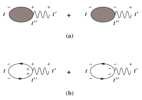
Figure 1: Feynman diagrams for the invariant photon production rate given by Eq. (4.7). Fig. (a) is in terms of the full self-energy of the photon to all orders in $\alpha_{s}$ and to order $\alpha$. Fig. (b) is the lowest order contribution, of order $\alpha$.

We focus on the lowest order (one-loop) contribution which, as has been shown in Ref. [19], is missed by all the previous investigations which use the $S$-matrix approach thus assuming an infinite QGP lifetime. In using bare quark propagators we consider the quark momentum in the loop to be hard, i.e., $q\gtrsim T_{i}$. Soft quark lines require hard thermal loop (HTL) resummed effective quark propagator [28] leading to higher order corrections. Indeed, the one-loop diagram with soft quark loop momentum is part of the higher order contribution of order $\alpha\alpha_{s}$ that has been calculated in Refs. [9, 10].

To lowest order in perturbation theory, the result for two light quark flavors ($u$ and $d$) reads [19]

$$E\frac{dN(t)}{d^{3}p\,d^{4}x} = \frac{2}{(2\pi)^{3}}\int_{t_{i}}^{t}dt^{\prime\prime}\int_{-\infty}^{+\infty}\frac{d\omega}{\pi}\,\mathcal{R}(\omega)\,\cos[(\omega-E)(t-t^{\prime\prime})],$$ (4.8)

with

$$\mathcal{R}(\omega) = \frac{20\,\pi^{2}\alpha}{3}\int\frac{d^{3}q}{(2\pi)^{3}}\Big{\{}2\big{[}1-({\hat{p}}\cdot{\hat{k}})({\hat{p}}\cdot{\hat{q}})\big{]}n(q)[1-n(k)]\,\delta(\omega+k-q)$$ (4.9)

$$+\big{[}1+({\hat{p}}\cdot{\hat{k}})({\hat{p}}\cdot{\hat{q}})\big{]}n(q)n(k)\,\delta(\omega-k-q)\Big{\}},$$

where $q=|{\vec{q}}|$, $k=|{\vec{p}}+{\vec{q}|}$ and $n(q)=1/[e^{q/T_{i}}+1]$ is the quark distribution function at the initial time $t_{i}$. The dependence of $\mathcal{R}(\omega)$ on the quark distribution at the initial time $t_{i}$ is a consequence of the fact that in nonequilibrium quantum field theory the important ingredient is the initial density matrix [27, 24, 25, 26], which consistent with hydrodynamics is taken to be thermal for quarks and gluons. Obviously $\mathcal{R}(\omega)$ vanishes if there is no “medium” hence this contribution to photon production is a result of the presence of the medium, which exists as a thermal bath for $t>t_{i}\sim 1~{}\mbox{fm}/c$.

At this stage we comment on how the assumption of neglecting the photon population can be relaxed. Allowing an initial as well as the buildup of the photon population leads to a full quantum kinetic equation of the form [24, 25, 26]

$$\frac{d}{dt}n_{\gamma}({\vec{p}},t)=\Gamma_{\text{gain}}({\vec{p}},t)[1+n_{\gamma}({\vec{p}},t)]-\Gamma_{\text{loss}}({\vec{p}},t)\,n_{\gamma}({\vec{p}},t),$$ (4.10)

where $n_{\gamma}({\vec{p}},t)=dN(t)/d^{3}pd^{3}x$, $\Gamma_{\text{gain}}$ is given by the right hand side of Eq. (4.8) divided by $E$, and $\Gamma_{\text{loss}}$ is obtained from $\Gamma_{\text{gain}}$ through the replacement $n\leftrightarrow 1-n$ of the quark distribution functions (to the order considered) [24, 25, 26]. The population at the time of onset of local thermodynamic equilibrium is a result of electromagnetic processes during the pre-equilibrium stage [22], i.e., $n_{\gamma}({\vec{p}},t_{0})\propto\alpha$, thus leading to higher order corrections in $\alpha$. Therefore, to lowest order in $\alpha$ the neglect of the $n_{\gamma}$ in the quantum kinetic equation is justified and leads to Eq. (4.8).

In the case of a nonexpanding and thermalized QGP, the integral over $t^{\prime\prime}$ in Eq. (4.8) can be carried out directly leading to

$$E\frac{dN(t)}{d^{3}p\,d^{4}x}=\frac{2}{(2\pi)^{3}}\int_{-\infty}^{+\infty}d\omega\,\mathcal{R}(\omega)\,\frac{\sin[(\omega-E)(t-t_{i})]}{\pi(\omega-E)},$$ (4.11)

A detailed analysis [19, 26] of $\mathcal{R}(\omega)$ shows that the first delta function $\delta(\omega+k-q)$ with support below the light cone ($\omega^{2}<E^{2}$) corresponds to the Landau damping cut, and the second delta function $\delta(\omega-k-q)$ with support above the light cone corresponds to the usual two-particle cut. Furthermore, $\mathcal{R}(\omega)$ has a clear physical interpretation in terms of the following energy nonconserving photon production processes: the first term describes (anti)quark bremsstrahlung $q(\bar{q})\rightarrow q(\bar{q})\gamma$, and the second term describes quark-antiquark annihilation to photon $q\bar{q}\rightarrow\gamma$. It has been shown in Ref. [19] that the dominant process for production of energetic photons is the (anti)quark bremsstrahlung. As explained in Ref. [19], in writing $\mathcal{R}(\omega)$, we have ignored the term corresponding to the “vacuum” process $0\rightarrow q\bar{q}\gamma$. The “vacuum” term, which persists for an infinitely long time, results in an energy conserving delta function that obviously vanishes.

At this stage we can make contact with the $S$-matrix calculation and highlight the importance of the finite-time, nonequilibrium analysis. If, as is implicit in the $S$-matrix calculation, the QGP is assumed in thermal equilibrium and with an infinite lifetime (entailing that $t_{i}\rightarrow-\infty$ and $t_{f}\to\infty$), then we can take the infinite time limit $t_{i}\to-\infty$ in the argument of the sine function in Eq. (4.11) and use the approximation

$$\frac{\sin[(\omega-E)t]}{\pi(\omega-E)}\buildrel t\rightarrow\infty\over{\approx}\delta(\omega-E).$$ (4.12)

This is the assumption of completed collisions that is invoked in time-dependent perturbation theory leading to Fermi’s golden rule and energy conservation. The delta function $\delta(\omega-E)$ is a manifestation of energy conservation for each completed collision. Under this assumption one finds a time-independent photon production rate proportional to $\mathcal{R}(E)$, provided that the latter is finite. In the present situation, however, the delta functions in $\mathcal{R}(\omega)$ cannot be satisfied on the photon mass shell. Therefore, under the assumption of completed collisions the lowest order energy nonconserving contribution to the photon production rate simply vanishes due to kinematics. Therefore this lowest order contribution is absent (by energy conservation) in the $S$-matrix calculation, but is present at any finite time.

The relevant question to ask is how this finite-time contribution of order $\alpha$ compares to the higher order $S$-matrix contribution to the photon yield.

The photon yield (per unit volume) is obtained by integrating the rate over the lifetime of the QGP. Using Eq. (4.11), one obtains

$$E\frac{dN}{d^{3}p~{}d^{3}x}=\frac{2}{(2\pi)^{3}}\int_{-\infty}^{+\infty}d\omega\,\mathcal{R}(\omega)\,\frac{1-\cos[(\omega-E)(t_{f}-t_{i})]}{\pi(\omega-E)^{2}},$$ (4.13)

where $t_{f}-t_{i}\sim 10\,{\rm fm}/c$ is the lifetime of the QGP. For $T_{i}\sim 200$ MeV, the following important results have been shown in Ref. [19].

• Direct photon production given by Eq. (4.13) features a power law spectrum for $E\gg T_{i}$ as a consequence of the energy nonconserving photon production processes: (anti)quark bremsstrahlung $q(\bar{q})\rightarrow q(\bar{q})\gamma$ and quark-antiquark annihilation $q\bar{q}\rightarrow\gamma$.

• The direct photon yield arising form this nonequilibrium finite-lifetime effect in the energy range $E>2$ GeV dominates over that obtained from equilibrium rate calculations given by Eq. (2.9) during the QGP lifetime.

• Furthermore the general analysis presented in Refs. [25, 19] shows that the general expression for the invariant rate given by Eq. (4.13) in terms of spectral representations is correct to all orders. In particular to lowest order in $\alpha$ but to all orders in $\alpha_{s}$ the spectral density $\mathcal{R}(\omega)=\alpha[\mathcal{R}^{(0)}(\omega)+\alpha_{s}\ln(1/\alpha_{s})\mathcal{R}^{(1)}(\omega)+\cdots]$, all terms enter with the same time dependence. In particular $\mathcal{R}^{(0)}(\omega)$ is given by Eq. (4.9) and $\mathcal{R}^{(1)}(\omega=E)$ is given by Eq. (2.9). In the limit $t_{f}-t_{i}\rightarrow\infty$ the terms with support at $\omega=E$ result in a photon yield that grows linearly with time, while the terms for which $\mathcal{R}(E)=0$ will grow in time much slower. In the infinite time limit those terms that do not vanish at $\omega=E$ lead to photon yield that grows linearly with time and hence a finite time-independent rate, while those that vanish will be subleading. However, for a finite time interval which terms in the perturbative expansion dominate will depend on the competition between the order in perturbation theory and the length of the time interval.

While these results in the nonexpanding case revealed the importance of the nonequilibrium and finite-lifetime aspects, the most experimentally relevant case to study is that of an expanding QGP. A constant rate obtained from the $S$-matrix calculation leads to a yield that will grow in time linearly, while as analyzed in Ref. [19] the lowest order nonequilibrium yield grows much slower (logarithmically).

Therefore the relevant question is which contribution is dominant during the lifetime of the QGP . This question can only be answered by a detailed numerical study of both yields which is performed below.

4.2 Longitudinally expanding QGP

As a prelude to photon production from an expanding QGP, and according with the usual approach [17, 18], we first focus on the invariant photon production rate from each individual fluid cell of the QGP. Since the proper time equals the local time in the local rest frame of any fluid cell, we can follow the same real-time nonequilibrium analysis presented in the proceeding subsection to calculate the nonequilibrium invariant photon production rate in the local rest frame of each fluid cell [17, 18]. We obtain [19, 26]

$$E\frac{dN(\tau)}{d^{3}p\,d^{4}x}\bigg{|}_{\rm LR} = \lim_{\tau^{\prime}\rightarrow\tau}\left(\frac{\partial}{\partial\tau^{\prime}}-iE\right)\sum^{N_{f}}_{f=1}\frac{e\,e_{f}}{2(2\pi)^{3}}\int\frac{d^{3}q}{(2\pi)^{3}}\big{\langle}\bar{\psi}_{f}^{-}(-{\vec{k}},\tau)$$ (4.14)

$$\times\,{\vec{\gamma}}\cdot{\vec{A}}^{+}_{T}({\vec{p}},\tau^{\prime})\psi_{f}^{-}({\vec{q}},\tau)\big{\rangle}+{\rm c.c.}.$$

As before, the nonequilibrium expectation values on the right-hand side of Eq. (4.14) is computed perturbatively to order $\alpha$ and in principle to all orders in $\alpha_{s}$ by using real-time Feynman rules and propagators. To lowest order in perturbation theory, the result for two light quark flavors ($u$ and $d$) reads

$$E\frac{dN(\tau)}{d^{3}p\,d^{4}x}\bigg{|}_{\rm LR} = \frac{2}{(2\pi)^{3}}\int_{\tau_{i}}^{\tau}d\tau^{\prime\prime}\int_{-\infty}^{+\infty}\frac{d\omega}{\pi}\,\mathcal{R}(\omega)\,\cos[(\omega-E)(\tau-\tau^{\prime\prime})],$$ (4.15)

where $\mathcal{R}(\omega)$ is the same as that given in Eq. (4.9), but now with $n(q)=1/[e^{q/T_{i}}+1]$ being the quark distribution function at initial proper time $\tau_{i}$, at which the QGP reaches local thermal equilibrium.

In principle in the case of an expanding QGP under consideration, the photon production rate given by Eq. (4.15) has to be supplemented by kinetic equations that describe the evolution of the quark and gluon distribution functions so as to setup a closed set of coupled equations. However the assumption of the validity of (ideal) hydrodynamics entails that the quarks and gluons form a perfectly coupled fluid. This in turn implies that the mean free paths of the quarks and gluons are much shorter than the typical wavelengths and the relaxation time scales are much shorter than the typical time scales, i.e., the quark and gluon distribution functions adjust to local thermal equilibrium instantaneously. Thus the assumption of the validity of (ideal) hydrodynamics bypasses the necessity of the coupled kinetic equations: quarks and gluons are in local thermal equilibrium at all times. Therefore, within the framework of hydrodynamics we obtain the invariant photon production rate by directly replacing the initial quark distribution function $n(q)$ in Eq. (4.9) by the “updated” distribution function $n[q,T(\tau^{\prime\prime})]=1/[e^{q/T(\tau^{\prime\prime})}+1]$ at proper time $\tau^{\prime\prime}>\tau_{i}$, where $T(\tau^{\prime\prime})$ is determined by the cooling law Eq. (3.3). The nonequilibrium invariant photon production rate that is consistent with the underlying hydrodynamics is then given by

$$E\frac{dN}{d^{3}p\,d^{4}x}\bigg{|}_{\rm LR}[\tau,E,T(\tau)] = \frac{2}{(2\pi)^{3}}\int_{\tau_{i}}^{\tau}d\tau^{\prime\prime}\int_{-\infty}^{+\infty}\frac{d\omega}{\pi}\,\mathcal{R}[\omega,T(\tau^{\prime\prime})]$$ (4.16)

$$\times\,\cos[(\omega-E)(\tau-\tau^{\prime\prime})],$$

with

$$\mathcal{R}[\omega,T(\tau)] = \frac{20\,\pi^{2}\alpha}{3}\int\frac{d^{3}q}{(2\pi)^{3}}\Big{\{}2\big{[}1-({\hat{p}}\cdot{\hat{k}})({\hat{p}}\cdot{\hat{q}})\big{]}n[q,T(\tau)]\bar{n}[k,T(\tau)]$$ (4.17)

$$\times\,\delta(\omega+k-q)+\big{[}1+({\hat{p}}\cdot{\hat{k}})({\hat{p}}\cdot{\hat{q}})\big{]}n[q,T(\tau)]n[k,T(\tau)]$$

$$\times\,\delta(\omega-k-q)\Big{\}},$$

where $n[q,T(\tau)]=1/[e^{q/T(\tau)}+1]$ and $\bar{n}=1-n$. The momentum $q$ integrals in Eq. (4.17) are calculated in the LR frame and hence are equivalent to those of the nonexpanding case above.

Before proceeding further, we emphasize two noteworthy features of the nonequilibrium invariant photon production rate: (i) The photon production processes do not conserve energy. (ii) The rate depends on (proper) time not only implicitly through the local temperature but also explicitly. Furthermore, this explicit (proper) time dependence is non-Markovian as clearly displayed in Eq. (4.16). Whereas these two features seem to be rather uncommon within the framework of the usual $S$-matrix approach to transport in heavy ion collisions [29], they are not unusual in quantum kinetics of nonrelativistic many-body systems [23, 30]. Indeed, energy nonconserving transitions and memory effects which cannot be explained by usual (energy conserving) Boltzmann kinetics have been observed recently in the ultrafast spectroscopy of semiconductors that are optically excited by a femtosecond laser pulse [31].

The real-time kinetic approach when incorporated consistently with hydrodynamics reveals clearly that photon production from an expanding QGP is inherently a nonequilibrium quantum effect associated with the finite lifetime of the QGP.

At RHIC and LHC energies the quark distribution function $n[q,T(\tau)]$ depends on the proper time $\tau$ very weakly through the temperature $T(\tau)$ within the lifetime of the QGP phase, hence a Markovian approximation (MA) in which the temperature in $\mathcal{R}[\omega,T(\tau^{\prime\prime})]$ is taken at the upper limit of the integral is reasonable and hence the memory kernel may be simplified. In this Markovian approximation, $\mathcal{R}[\omega,T(\tau^{\prime\prime})]$ in Eq. (4.16) is replaced by $\mathcal{R}[\omega,T(\tau)]$ and taken outside of the $\tau^{\prime\prime}$-integral. Thus Eq. (4.16) becomes

$$E\frac{dN}{d^{3}p\,d^{4}x}\bigg{|}^{\rm MA}_{\rm LR}[\tau,E,T(\tau)] = \frac{2}{(2\pi)^{3}}\int_{-\infty}^{+\infty}d\omega\,\mathcal{R}[\omega,T(\tau)]$$ (4.18)

$$\times\,\frac{\sin[(\omega-E)(\tau-\tau_{i})]}{\pi(\omega-E)}.$$

A computational advantage of this Markovian nonequilibrium production rate is that it provides the “updated” quark distribution functions locally in time. Physically, the motivation for this approximation is that the most important aspect of the nonequilibrium effect is the nonconservation of energy (i.e., off-shellness) originated in the finite lifetime of the QGP, a feature that is missed by the usual $S$-matrix calculation, while the proper time variation of the temperature is a secondary effect and accounted for in the $S$-matrix approach.

It is worth noting that a connection with the Boltzmann approximation can be obtained by assuming completed collisions, i.e., taking the limit $\tau_{i}\rightarrow-\infty$ in the argument of the sine function in Eq. (4.18) and using the approximation given by Eq. (4.12). Consequently, the lowest order nonequilibrium photon production rate vanishes in the Boltzmann approximation due to kinematics. This highlights, once again, that the usual approach to photon production outlined in Sec. 2 and used in the literature corresponds to the Boltzmann approximation and therefore fails to capture the energy nonconserving and memory effects that occur during the transient stage of evolution of the QGP.

We are now in a position to calculate the direct photon yield from a longitudinally expanding QGP. In the CM frame the invariant production rate for photons of four-momentum $P^{\mu}$ from a fluid cell with four-velocity $u^{\mu}$ can be obtained from Eq. (4.18) through the replacement $E\rightarrow P^{\mu}u_{\mu}$. In terms of the photon transverse momentum $p_{T}$ and rapidity $y$, one finds $P^{\mu}u_{\mu}=p_{T}\cosh(y-\eta)$. The photon yield is obtained by integrating the nonequilibrium rate over the space-time evolution of the expanding QGP. Assuming a central collision of identical nuclei, in the Markovian approximation we find the invariant nonequilibrium photon yield to lowest order in perturbation theory to be given by

$$\frac{dN}{d^{2}p_{T}\,dy}\bigg{|}^{\rm MA}_{\rm CM} = \pi R_{A}^{2}\int_{\tau_{i}}^{\tau_{f}}d\tau\,\tau\int_{-\eta_{\rm cen}}^{\eta_{\rm cen}}d\eta\,E\frac{dN}{d^{3}p\,d^{4}x}\bigg{|}^{\rm MA}_{\rm LR}[\tau,P^{\mu}u_{\mu},T(\tau)],$$ (4.19)

where $R_{A}$ is the radius of the nuclei and $-\eta_{\rm cen}<\eta<\eta_{\rm cen}$ denotes the central rapidity region within which Bjorken’s hydrodynamical model is valid.

As remarked above, at RHIC and LHC energies the quark distribution function $n[q,T(\tau)]$ depends on the proper time $\tau$ very weakly through the temperature $T(\tau)$ within the lifetime of the QGP phase, therefore the resultant photon yield is expected to qualitatively resemble the nonequilibrium photon yield from a nonexpanding QGP studied in Ref. [19]. This will be numerically verified below. We note that the expanding and nonexpanding cases differ mainly by the Jacobian $\tau$ in the $\tau$ integral in Eq. (4.19) that accounts for the longitudinal expansion of the QGP, and by the replacement $E\rightarrow P^{\mu}u_{\mu}$ in the argument of the invariant photon production rate that accounts for the shift of the photon energy under local Lorentz boost.

Figure 2: Comparison of nonequilibrium (solid) and equilibrium (dotted) photon yields at midrapidity ($y=0$) from a longitudinally expanding QGP at RHIC energies with initial conditions given by $\tau_{i}=1$ fm/$c$ and $T_{i}=200$ (top), 300 (bottom) MeV.

4.3 Numerical analysis: central collisions at RHIC and LHC energies

We now perform a numerical analysis of the nonequilibrium photon yield and compare the results to the equilibrium one obtained from higher order equilibrium rate calculations given by Eq. (2.9). The nonequilibrium photon yield in the Markovian approximation given by Eq. (4.19) contains a four-dimensional integral that is performed numerically for the values of parameters of relevance at RHIC and LHC energies.

For central ¹⁹⁷Au$+{}^{197}$Au collisions at RHIC energies $\sqrt{s}\sim 200A$ GeV, we take $R_{A}\simeq 1.2\,A^{1/3}$ fm $\approx 7$ fm [15] and $\eta_{\rm cen}=2$. The initial thermalization time is taken to be $\tau_{i}=1$ fm/$c$ [18, 20], the final proper time $\tau_{f}$ is determined when the critical temperature for the quark-hadron transition is reached at $T(\tau_{f})\simeq 160$ MeV and is obtained from the cooling law given by Eq. (3.3) for a given initial temperature $T_{i}$ at proper time $\tau_{i}$.

The nonequilibrium photon yield at midrapidity ($y=0$) in the range of transverse momentum $T_{i}<p_{T}<5$ GeV/$c$ is shown on a log-log plot in Fig. 2 for initial temperatures $T_{i}=200$ and 300 MeV. For comparison we also plot the corresponding equilibrium yield obtained by integrating Eq. (2.9) with the transformation to the CM frame as specified by Eq. (3.5), and using the value of $\alpha_{s}$ [17, 18, 32]

$$\alpha_{s}[T(\tau)]=\frac{6\pi}{(33-2N_{f})\ln[8\,T(\tau)/T_{c}]},$$ (4.20)

with $N_{f}=2$. Furthermore, Figure 3 shows the rapidity distribution of the nonequilibrium photon yield at different values of $p_{T}$ for $T_{i}=200$ and $300$ MeV. Several noteworthy features are gleaned from these figures:

Figure 3: Rapidity distribution of the nonequilibrium photon yield at $p_{T}=1$ (solid), 2 (dotted), and 3 (dashed) GeV for a longitudinal expanding QGP at RHIC energies with initial conditions given by $\tau_{i}=1\,{\rm fm}/c$ and $T_{i}=200$ (top), 300 (bottom) MeV. The distribution is symmetric at $y=0$.

• Whereas the equilibrium yield dominates the total yield for small $p_{T}$, the nonequilibrium yield becomes significantly dominant in the range $p_{T}>1.0-1.5$ GeV/$c$. Perhaps coincidentally, this is the range in which the CERN WA98 data for central Pb$+$Pb collisions at SPS energies shows a distinct excess [1].

• While the equilibrium yield leads to a transverse momentum distribution that falls off approximately with the Boltzmann factor $e^{-p_{T}/T_{i}}$, the nonequilibrium yield is not Boltzmann suppressed and falls off algebraically. It is found numerically that for $p_{T}\gg T_{i}$ and within the region $1\lesssim p_{T}\lesssim 5$ GeV/$c$ the nonequilibrium yield at midrapidity falls off with a power law $p_{T}^{-\nu}$ with $\nu\simeq 2.47$ and $2.77$ for $T_{i}=200$ and 300 MeV, respectively. This is a remarkable consequence of the fact that bremsstrahlung is the dominant process. As discussed in detail in Ref. [19] at large energies the dominant process is bremsstrahlung corresponding to the contribution from the term $n(q)[1-n(k)]$ with $k=|{\vec{p}}+{\vec{q}}|$ in Eq. (4.9). For large photon energy $p$ the important contribution, which is not exponentially suppressed arises from the small $q$ region.

• A central plateau in the range of rapidity $y\lesssim 2$ is seen clearly. The rapidity distribution begins to bend down when $y\simeq\eta_{\rm cen}$, i.e., when the photon rapidity probes the fragmentation region.

• The numerical analysis of the expanding case reveals features very similar to those found in the nonexpanding case studied in Ref. [19], where we estimate that for $p_{T}\geq 1.5$ GeV/$c$ the higher order equilibrium contribution to the direct photon yield (which grows linearly in time) becomes of the same order as the lowest order nonequilibrium contribution (which grows at most logarithmically in time) only if the lifetime of the QGP is of the order longer than 1000 fm/$c$. Therefore, we conclude that these nonequilibrium effects dominate during the lifetime of the QGP in a realistic ultrarelativistic heavy ion collision experiment.

Figure 4: Comparison of nonequilibrium (solid) and equilibrium (dotted) photon yields at midrapidity ($y=0$) from a longitudinally expanding QGP at LHC energies with initial conditions given by $\tau_{i}=1$ fm/$c$ and $T_{i}=450$ (top), 500 (bottom) MeV.

Similar numerical analysis can be performed for central ²⁰⁸Pb$+{}^{208}$Pb collisions at higher LHC energies $\sqrt{s}\sim 5500A$ GeV, for which we take $R_{A}\approx 7$ fm, $\eta_{\rm cen}=5$ and $\tau_{i}=1$ fm/$c$ [18, 20]. The comparison of nonequilibrium and equilibrium photon yields at midrapidity is displayed in Fig. 4 for $T_{i}=450$ and 500 MeV. The dominance of the nonequilibrium yield at high $p_{T}$ remains but now at higher transverse momentum $p_{T}\gtrsim 2$ GeV. This can be understood as a consequence of the longer QGP lifetime resulting from higher initial temperature at LHC energies. Furthermore, it is found numerically that for $1\lesssim p_{T}\lesssim 5$ GeV/$c$ the nonequilibrium yield at midrapidity falls off with a power law $p_{T}^{-\nu}$ with $\nu\simeq 2.52$ and $2.56$ for $T_{i}=450$ and 500 MeV, respectively.

These results indicate a clear manifestation of the nonequilibrium aspects of direct photon production associated with a transient QGP of finite lifetime. The most experimentally accessible signal of the nonequilibrium effects revealed by this analysis is the power law falloff of the transverse momentum distribution for direct photons in the range $1\lesssim p_{T}\lesssim$ 5 GeV/$c$ with an exponent $2.5\lesssim\nu\lesssim 3$ for temperatures expected at RHIC and LHC energies. Our numerical studies reveal that this exponent increases with initial temperature and therefore with the initial energy density of the QGP and the total multiplicity rapidity distribution $dN_{\pi}/dy$ [20]. This could be a clean experimental nonequilibrium signature of a transient QGP since the photon distribution from the hadronic gas is expected to feature a Boltzmann type exponential suppression for $p_{T}\gg T_{i}$ [9, 16, 17, 18].

5 Conclusions and discussions

Our goal in this article is to search for clear experimental signatures of direct photons associated with nonequilibrium aspects of the transient quark-gluon plasma created in ultrarelativistic heavy ion collisions at RHIC and LHC energies.

We argue that the usual $S$-matrix approach to direct photon production from an expanding nonequilibrium QGP has conceptual limitations. Instead, we introduce a real-time kinetic approach that allows a consistent treatment of photon production from a transient nonequilibrium state of finite lifetime.

We focus on obtaining the direct photon yield from a thermalized QGP undergoing Bjorken’s hydrodynamical expansion in central Au$+$Au collisions at RHIC ($\sqrt{s}\sim 200A$ GeV) and LHC ($\sqrt{s}\sim 5500A$ GeV) energies. The lifetime of a QGP for these collisions is of order $\lesssim 10-30$ fm/$c$. We find that (anti)quark bremsstrahlung $q(\bar{q})\rightarrow q(\bar{q})\gamma$ and quark-antiquark annihilation $q\bar{q}\rightarrow\gamma$, both of lowest order in $\alpha$, dominate during such short time scales, with bremsstrahlung dominating for $p_{T}\gg T_{i}$. The contribution from these processes is a consequence of the transient nature and the finite lifetime of the QGP. As compared to the equilibrium rate calculations, these processes lead to a substantial enhancement in direct photon production for $1-2\lesssim p_{T}\lesssim$ 5 GeV/$c$ near midrapidity. In striking contrast with the equilibrium calculation that predicts an exponential suppression of the transverse momentum distribution for $p_{T}\gg T_{i}$ ($T_{i}$ is the initial temperature), the nonequilibrium processes lead to a power law behavior instead. We find that at RHIC and LHC energies the direct photon transverse momentum distribution near midrapidity is of the form $p^{-\nu}_{T}$ with $2.5\lesssim\nu\lesssim 3$ for $1\lesssim p_{T}\lesssim$ 5 GeV/$c$ and that photon rapidity distribution (for fixed $p_{T}$) is almost flat in the interval $|y|\lesssim\eta_{\rm cen}$, where $|\eta|<\eta_{\rm cen}$ denotes the central rapidity region of the QGP. The exponent $\nu$ is numerically found to increase with the initial temperature, hence increases with the total multiplicity rapidity distribution $dN_{\pi}/dy$, which is an experimental observable.

Thus, as the main conclusion, we propose that direct photons could potentially provide distinct experimental signatures of the transient nonequilibrium QGP created at RHIC and LHC energies, both in the form of a large enhancement at $1-2\lesssim p_{T}\lesssim$ 5 GeV/$c$ as well as a power law transverse momentum distribution $p^{-\nu}_{T}$ with an exponent $\nu$ that is within the range $2.5\lesssim\nu\lesssim 3$ and increases with total multiplicity rapidity distribution $dN_{\pi}/dy$.

Discussions.

• Our study of direct photon production focuses solely on the QGP phase and neglects contributions from pre-equilibrium stage as well as the mixed and hadronic phases, because we focus on a comparison between the usual equilibrium approach and the kinetic real-time approach. While the usual equilibrium approach treats the thermalized state as stationary, the real time kinetic approach allows to follow the time evolution of the density matrix as an initial value problem consistent with hydrodynamics. Furthermore, as discussed elsewhere in the literature, since most of the high-$p_{T}$ photons originate from the very early, hot stage in the QGP phase [8, 9, 11, 14] and photons produced in the mixed phase as well as the subsequent hadronic phase are mainly in the lower-$p_{T}$ region [18], the nonequilibrium yield from the QGP phase contributes dominantly to the total high-$p_{T}$ photons.

• While we have provided a systematic real-time description compatible with the initial value problem associated with hydrodynamic evolution, more needs to be understood for a complete description of all the different stages. The parton cascade approach to describe the early pre-equilibrium stage after the collision is an important first step in a full microscopic description, but perhaps a more consistent description of the initial condition for QGP formation must be based on the recent notions of a color glass condensate [35, 36]. Hence, a complete treatment of the direct photon yield must, in principle, begin from the initial stage, possibly a color glass condensate, and obtain the real-time evolution of photon production. Clearly there must be many more advances in this field before such a program becomes feasible. The finite-temperature equilibrium calculations assume that the equilibrium thermal state always prevailed, thus ignores completely not only the initial stages but also the time evolution. Our approach while incorporating the time evolution during the stage of local thermodynamic equilibrium consistently, also neglects the initial stage. However, the advantage of our method is that if there is an estimate for the photon distribution at the onset of thermalization we could evolve the full quantum kinetic equation, including the higher order corrections in $\alpha$ as discussed in the text. We have focused on direct photons from a transient QGP for a direct comparison with equilibrium calculations, but obviously photons will continue to be produced during the mixed and hadronic phases. A detailed understanding of the phase transition as well as the hadronic photon production matrix elements is necessary for a more reliable estimate of the potential nonequilibrium effects after hadronization.

• Although we do not claim to have provided a completely detailed understanding of potential nonequilibrium effects due to the lack of knowledge of initial conditions in heavy ion collisions, we do claim that our approach provides a more systematic description of the finite-lifetime effects associated with a transient QGP. These effects lead to a distinct experimental prediction: a power law falloff of the distribution $dN/d^{2}p_{T}dy$ near the central rapidity region which is distinguishable from a thermal tail for $1-2\lesssim p_{T}\lesssim 5$ GeV/$c$. We also note that the parton cascade results of Srivastava and Geiger [22] also seem to reveal a power law falloff of the photon distribution in this range of momentum with a similar amplitude and comparable exponent, as can be gleaned from Figs. 2 and 3 of Ref. [22]. Perhaps these two effects, namely the pre-equilibrium prompt photons and the direct photons from a hydrodynamically expanding QGP with a finite lifetime cannot be distinguished experimentally. Nevertheless, we emphasize that a power law departure from a thermal tail in the direct photon spectrum may very well be explained by nonequilibrium effects, either by a finite QGP lifetime as advocated in this article or by prompt photons from the pre-equilibrium stage.

• As many recent investigations [33, 34] have suggested that the QGP produced at RHIC and LHC energies is not expected to be in local chemical equilibrium, i.e., the distribution functions of quarks and gluons will probably be undersaturated. An important extension of our work will be the study of nonequilibrium effects on direct photon production from a chemically nonequilibrated QGP.

• Transient QGP vs high energy particle collisions. An important and very relevant question is that why not treat high energy particle collisions in the same manner, i.e., with the real-time evolution rather than with the $S$-matrix approach. The answer to this question hinges on the issue of time scales. In a typical high energy particle collider experiment, the colliding “beams” are actually bunches or packets with a typical spatial extent of order $1-10$ cm and hence the typical total time interval for the collision is of order $10^{-9}$ sec [37]. This time scale is many orders of magnitude longer than the typical hadronic interaction time scale $\sim 10^{-23}$ sec, thus taking the infinite time limit is amply justified. This, of course, is the basis for using the $S$-matrix calculation in terms of asymptotic in and out states (at $t=\mp\infty$): the total interaction time ($t_{f}-t_{i}$) is much, much longer than the typical hadronic time scale. With regard to the heavy ion collision, the consensus is that after an initial pre-equilibrium stage, a locally thermalized QGP is formed. It then evolves hydrodynamically, hadronizes and eventually the freeze-out of the hadronic gas ensues. Current theoretical estimates at RHIC energies indicate a total time between formation and freeze-out of order $50-100$ fm/$c$, with a QGP phase lasting for about $10$ fm/$c$. These time scales, at least the lifetime of the QGP, are not several orders of magnitude larger than the hadronic interaction time scale, thus the infinite time limit taken in the $S$-matrix calculation is at best questionable. Therefore while in typical particle collider experiments the $S$-matrix approach is valid (as has been demonstrated by over half a century of experiments!), the transient QGP with a finite lifetime of the order of the hadronic time scales merits a different treatment, which is the point of this article.

• An important and related aspect that requires further investigation is the finite size of the QGP. Much in the same way as the finite lifetime introduces nonequilibrium effects associated with energy nonconserving transitions, we expect that the finite size $\sim 7$ fm of the QGP will introduce uncertainty in the momentum of the emitted particles. This is clearly an important topic that deserves further and deeper study but is beyond the scope of this article. However, at this stage we speculate that if such effects are present they could bear an imprint in transverse flow.

Work along many of these directions is currently in progress.

Appendix A Photon production rate and current correlation function

The equilibrium thermal photon production rate is related to the Fourier transform of the thermal expectation value of the quark electromagnetic current correlation function [6, 8, 14]. In this appendix we show that the photon production rate given by Eq. (4.7) is related to the Fourier transform of the nonequilibrium expectation value of the quark electromagnetic current correlation function.

In terms of the (Abelian) gauge invariant fields the interaction Lagrangian between quarks and photons reads [26]

$$\mathcal{L}_{\rm int}=e\,{\vec{J}}\cdot{\vec{A}}_{T},$$ (A.1)

with ${\vec{A}}_{T}$ the transverse component of the photon field and ${\vec{J}}$ the spatial component of the quark electromagnetic current

$${\vec{J}}=\sum^{N_{f}}_{f=1}\,e_{f}\,\bar{\psi}_{f}{\vec{\gamma}}\psi_{f}.$$ (A.2)

The invariant photon production rate given by Eq. (4.7) can be written in terms of ${\vec{J}}$ as

$$E\frac{dN(t)}{d^{3}p\,d^{4}x} = \lim_{t^{\prime}\rightarrow t}\frac{e}{2(2\pi)^{3}}\left(\frac{\partial}{\partial\tau^{\prime}}-iE\right)\left\langle{\vec{J}}^{-}(-{\vec{p}},t)\cdot{\vec{A}}^{+}_{T}({\vec{p}},t^{\prime})\right\rangle+{\rm c.c.}.$$ (A.3)

It is convenient to introduce the Fourier transform of the transverse component of the quark current correlation function $W_{T}^{\mbox{\scriptsize\raisebox{1.8pt}{\raisebox{1.8pt}{$\scriptscriptstyle>$} \raisebox{-1.0pt}{$\scriptscriptstyle\!\!\!\!\!\!<$}}}}(\omega,p)$ defined by

$$\frac{1}{2}\,\mathcal{P}^{ij}({\hat{p}})\left\langle J^{i+}({\vec{p}},t)J^{j-}(-{\vec{p}},t^{\prime})\right\rangle = \int^{+\infty}_{-\infty}\frac{d\omega}{2\pi}\,W_{T}^{<}(\omega,p)\,e^{-i\omega(t-t^{\prime})},$$ (A.4)

$$\frac{1}{2}\,\mathcal{P}^{ij}({\hat{p}})\left\langle J^{i-}({\vec{p}},t)J^{j-}(-{\vec{p}},t^{\prime})\right\rangle = \int^{+\infty}_{-\infty}\frac{d\omega}{2\pi}\,\big{[}W_{T}^{>}(\omega,p)\theta(t^{\prime}-t)$$ (A.5)

$$+\,W_{T}^{<}(\omega,p)\theta(t-t^{\prime})\big{]}\,e^{-i\omega(t-t^{\prime})},$$

where $\mathcal{P}^{ij}({\hat{p}})=\delta^{ij}-\hat{p}^{i}\hat{p}^{j}$ is the transverse projector. A diagrammatic expansion [see Fig. 1(a)] shows that to order $\alpha$ and to all orders in $\alpha_{s}$ Eq. (A.3) can be expressed in terms of $W^{<}(\omega,p)$ as

$$E\frac{dN(t)}{d^{3}p\,d^{4}x} = \frac{e^{2}}{(2\pi)^{3}}\int_{t_{i}}^{t}dt^{\prime\prime}\int^{+\infty}_{-\infty}\frac{d\omega}{2\pi}\,W_{T}^{<}(\omega,p)\,e^{-i(E-\omega)(t-t^{\prime\prime})}+{\rm c.c.},$$ (A.6)

where use has been made of the vacuum photon propagators. For a QGP with an initial state at time $t_{i}$ described by a thermal density matrix, one can show that the perturbative Kubo-Martin-Schwinger (KMS) condition holds to all orders in $\alpha_{s}$, i.e.,

$$W_{T}^{<}(\omega,p)=e^{-\omega/T_{i}}\,W_{T}^{>}(\omega,p),$$ (A.7)

where $T_{i}$ is the initial temperature. Consequently, one finds to all orders in $\alpha_{s}$ that $W_{T}^{<}(\omega,p)$ is a real quantity and related to the imaginary part of the retarded photon self-energy. Therefore Eq. (A.6) becomes

$$E\frac{dN(t)}{d^{3}p\,d^{4}x} = \frac{2e^{2}}{(2\pi)^{3}}\int_{t_{i}}^{t}dt^{\prime\prime}\int^{+\infty}_{-\infty}\frac{d\omega}{2\pi}\,W_{T}^{<}(\omega,p)\,\cos[(\omega-E)(t-t^{\prime\prime})],$$ (A.8)

which is correct to order $\alpha$ and to all orders in $\alpha_{s}$. This result generalizes that of Refs. [6, 8, 14] to the nonequilibrium situation in the real-time formulation. Upon comparing Eq. (A.8) with Eq. (4.8), one finds

$$\mathcal{R}(\omega)=\frac{e^{2}}{2}\left.W_{T}^{<}(\omega,p)\right|_{\text{one-loop}}.$$ (A.9)

References

- [1] WA98 Collaboration, M.M. Aggarwal et al., Phys. Rev. Lett. 85, 3595 (2000); nucl-ex/0006007.
- [2] B. Müller, The Physics of Quark-Gluon Plasma (Springer, Heidelberg, 1985); C.-Y. Wong, Introduction to High-Energy Heavy-Ion Collisions (World Scientific, Singapore, 1994); J.W. Harris and B. Müller, Annu. Rev. Nucl. Part. Sci. 46, 71 (1996).
- [3] K. Geiger, Phys. Rep. 258, 237 (1995); X.-N. Wang, 280, 287 (1997).
- [4] FOPI Collaboration, F. Rami et al., Phys. Rev. Lett. 84, 1120 (2000).
- [5] For instance, see J.-P. Blaizot, Nucl. Phys. A661, 3 (1999).
- [6] E.L. Feinberg, Nuovo Cim. 34A, 391 (1976).
- [7] E. Shuryak, Phys. Lett. B 78, 150 (1978); B. Sinha, 128, 91 (1983).
- [8] L.D. McLerran and T. Toimela, Phys. Rev. D 31, 545 (1985).
- [9] J.I. Kapusta, P. Lichard, and D. Seibert, Phys. Rev. D 44, 2774 (1991); 47, 4171 (1993).
- [10] R. Baier, H. Nakkagawa, A. Niégawa, and K. Redlich, Z. Phys. C 53, 433 (1992).
- [11] P.V. Ruuskanen, in Particle Production in Highly Excited Matter, NATO ASI Series, Series B: Physics Vol. 303, edited by H.H. Gutbrod and J. Rafelski (Plenum Press, New York, 1992).
- [12] P. Aurenche, F. Gelis, R. Kobes, and H. Zaraket, Phys. Rev. D 58, 085003 (1998).
- [13] The values of the numerical coefficients and are taken from F.D. Steffen and M.H. Thoma, Phys. Lett. B 510, 98 (2001). In this reference, it is pointed out that those values calculated in Ref. [12] were overestimated by a factor of 4 due to an error in the numerical codes.
- [14] C. Gale and J.I. Kapusta, Nucl. Phys. B357, 65 (1991).
- [15] M. Le Bellac, Thermal Field Theory (Cambridge University Press, Cambridge, England, 1996).
- [16] J. Sollfrank, P. Huovinen, M. Kataja, P.V. Ruuskanen, M. Prakash, and R. Venugopalan, Phys. Rev. C 55, 392 (1997).
- [17] D.K. Srivastava and B. Sinha, Phys. Rev. Lett. 73, 2421 (1994); nucl-th/0006018; D.K. Srivastava, Eur. Phys. J. C 10, 487 (1999).
- [18] J. Alam, S. Sarkar, T. Hatsuda, T.K. Nayak, and B. Sinha, Phys. Rev. C 63, 021901 (2001); J. Alam, S. Sarkar, P. Roy, T. Hatsuda, and B. Sinha, Ann. Phys. 286, 159 (2001).
- [19] S.-Y. Wang and D. Boyanovsky, Phys. Rev. D 63, 051702 (2001).
- [20] J.D. Bjorken, Phys. Rev. D 27, 140 (1983).
- [21] J.-P. Blaizot and J.-Y. Ollitrault, in Quark-Gluon Plasma 1, edited by R.C. Hwa (World Scientific, Singapore, 1990).
- [22] D.K. Srivastava and K. Geiger, Phys. Rev. C 58, 1734 (1998).
- [23] S.M. Alamoudi, D. Boyanovsky, H.J. de Vega, and R. Holman, Phys. Rev. D 59, 025003 (1999).
- [24] D. Boyanovsky, I.D. Lawrie, and D.-S. Lee, Phys. Rev. D 54, 4013 (1996); D. Boyanovsky, H.J. de Vega, R. Holman, S.P. Kumar, and R.D. Pisarski, 58, 125009 (1998).
- [25] D. Boyanovsky and H.J. de Vega, Phys. Rev. D 59, 105019 (1999); D. Boyanovsky, H.J. de Vega, and S.-Y. Wang, 61, 065006 (2000).
- [26] S.-Y. Wang, D. Boyanovsky, H.J. de Vega, and D.-S. Lee, Phys. Rev. D 62, 105026 (2000).
- [27] J. Schwinger, J. Math. Phys. 2, 407 (1961); L.V. Keldysh, JETP 20, 1018 (1965); K.-C. Chou, Z.-B. Su, B.-L. Hao, and L. Yu, Phys. Rep. 118, 1 (1985); D. Boyanovsky, H.J. de Vega and R. Holman, in Proceedings of the Second Paris Cosmology Colloquium, Observatoire de Paris, 1994, edited by H.J. de Vega and N. Sánchez (World Scientific, Singapore, 1995).
- [28] E. Braaten and R.D. Pisarski, Nucl. Phys. B337, 569 (1990); B339, 310 (1990); R.D. Pisarski, Physica A 158, 146 (1989); Phys. Rev. Lett. 63, 1129 (1989); Nucl. Phys. A525, 175 (1991).
- [29] C. Greiner, K. Wagner, and P. G. Reinhard, Phys. Rev. C 49, 1693 (1994); J. Rau and B. Müller, Phys. Rep. 272, 1 (1996).
- [30] For instance, see H. Haug and A.P. Jauho, Quantum Kinetics in Transport and Optics of Semiconductors (Springer, New York, 1998); J. Shah, Ultrafast Spectroscopy of Semiconductors and Semiconductor Nanostructures (Springer, New York, 1999).
- [31] L. Bányai, D.B. Tran Thoai, E. Reitsamer, H. Haug, D. Steinbach, M.U. Wehner, M. Wegener, T. Marschner, and W. Stolz, Phys. Rev. Lett. 75, 2188 (1995); S. Bar-Ad, P. Kner, M.V. Marquezini, D.S. Chemla, and K. El Sayed, 77, 3177 (1996); C. Fürst, A. Leitenstorfer, A. Laubereau, and R. Zimmermann, 78, 3733 (1997).
- [32] F. Karsch, Z. Phys. C 38, 147 (1988).
- [33] E. Shuryak, Phys. Rev. Lett. 68, 3270 (1992); T.S. Biró, E. van Doorn, B. Müller, M.H. Thoma, and X.-N. Wang, Phys. Rev. C 48, 1275 (1993).
- [34] E. Shuryak and L. Xiong, Phys. Rev. Lett. 70, 2241 (1993); M.H. Thoma and C.T. Traxler, Phys. Rev. C 53, 1348 (1996); M.G. Mustafa and M.H. Thoma, 62, 014902 (2000).
- [35] L. McLerran, hep-ph/0104285; hep-ph/9705426; E. Iancu, hep-ph/0010317.
- [36] A. Krasnitz and R. Venugopalan, hep-ph/0104168; hep-ph/0102118.
- [37] D.B. thanks colleagues from CDF, CLEO, and Hall D (Jefferson Lab) for educating him on these subtle but important aspects of collider physics.