Abstract

A two-component model is developed for diffractive electroproduction of $\rho^{0}$, $\phi$ and $J\!/\!\Psi$, based on non-perturbative and perturbative two-gluon exchange. This provides a common kinematical structure for non-perturbative and perturbative effects, and allows the role of the vector-meson vertex functions to be explored independently of the production dynamics. A good global description of the vector-meson data is obtained.

1 Introduction

High-energy exclusive photo- and electroproduction of vector mesons offers a variety of insights into the diffractive mechanism. The choice of different vector mesons and a range of photon virtualities allows one to move from the primarily nonperturbative regime to the primarily perturbative within one framework, and to explore kinematical regions where neither is predominant. Vector-meson production also has the benefit of a high rate, but it has the disadvantage of dependence on the choice of the vertex functions which couple the vector mesons to the $q\bar{q}$ pairs. In both respects it differs from deep virtual Compton scattering, which is theoretically better defined but has the disadvantage of a small cross section.

On the basis of the factorisation theorem [1], exclusive vector meson production can be considered as three separate processes: the fluctuation of the (virtual) photon into a $q\bar{q}$ pair; the interaction of the $q\bar{q}$ pair with the proton; and the formation of the vector meson from the $q\bar{q}$ pair which naturally involves the vector-meson vertex function. It may be argued that the structure of the nonpertubative vector-meson vertex function invalidates the proof of the factorisation theorem as it leads to additional contributions. However it has been shown [2], at least in a simple model for the vertex function, that gauge invariance ensures that the additional contributions cancel and factorisation is preserved.

The aim of this paper is twofold: to obtain a global description of exclusive vector meson photo- and electroproduction; and to explore the choice of vertex function.

The interaction of the $q\bar{q}$ pair with the pomeron is modelled by two-gluon exchange, figure 1, which can be applied both to nonperturbative and perturbative gluon exchange. The former is based on the model of Diehl [3] and the latter either by utilising the gluon structure function or following the model of Cudell and Royon [4].

The approach has the advantage of providing a common kinematical structure in which it is possible to separate the part of the vector-meson production amplitude describing the kinematics from the part which describes the dynamics of the process [5]. This separation then allows the nonpertubative and perturbative contributions to be combined at the amplitude level. Thus the approach follows recent ideas about two pomerons and two-component models of diffraction [6] through [12], combining “soft” (nonperturbative) and “hard” (perturbative) terms. This is essential for a global approach as neither a nonperturbative nor a perturbative model alone can describe all the observed features of diffractive vector-meson photo- and electroproduction.

In a previous paper [5] we have successfully applied this approach to calculate $\rho$ electroproduction in a model which avoids the vertex function complication, following [13], by considering open $q\bar{q}$-pair production with the invariant mass of the $q\bar{q}$ pair restricted to the region of the $\rho$ mass. However this method cannot be applied to higher-mass vector mesons: for a $q\bar{q}$ with an invariant mass in the region of the $\rho$ there are no states available except the $\rho$ itself (making a $10\%$ allowance for $\omega$ production), but this is not true for the $\phi$ and $J/\psi$. To obtain a global description of $\rho$, $\phi$ and $J/\psi$ photo- and electroproduction a kinematical framework involving vector-meson vertex functions has to be used.

In figure 1 the quark lines marked with a cross are off-shell, and the vertex function must necessarily take this into account. We use the prescription of Cudell and Royon [4] for these vertex functions. They appear very different from the usual on-shell vertex functions, for example those of Brodsky and Lepage [14]. However they are both obtained by a boost of the same vertex function from the vector-meson centre-of-mass and differ only by the imposition or relaxation of the on-shell condition.

Kinematical and dynamical considerations of the two-gluon exchange model are coverd in sections 2 and 3 and the vector-meson vertex functions are discussed in section 4. The model is applied to the data in section 5, and conclusions are given in section 6.

Figure 1: Two of the four vector meson production diagrams in the kinematical framework of Cudell and Royen [4]. The other two diagrams differ by reversal of the quark charge flow and give the same contribution to the cross section. The off-shell quarks are marked by crosses, dashed lines indicate cuts along which the quark lines are put on-shell, the minus sign indicates the momentum of an antiparticle.

2 The Kinematical Framework

The kinematical framework of our gluon exchange models is depicted in figure 1 and was developed by Cudell and Royen [4]. As noted earlier, it involves the vector-meson vertex function $\Phi\left(\ell\right)$ with either the quark or the anti-quark off-shell. The various four momenta used in our discussion are also defined in figure 1. In terms of them, the photon virtuality $Q^{2}=-q^{2}$ and the squared centre of mass energy of the photon-proton pair $W^{2}=(p+q)^{2}$. The traces corresponding to the $q\overline{q}$-loop in diagrams (a) and (b) of figure 1 are given by

$${\mathcal{T}}_{\mathbf{a}}^{\mu\nu} = Tr\Big{\{}\Phi\left(\ell\right)\left(\gamma.e\right)\left(m_{q}+\gamma.\left[\ell+{\textstyle{1\over 2}}V\right]\right){\gamma}^{\nu}\left(m_{q}+\gamma.\left[q+k+\ell-{\textstyle{1\over 2}}V\right]\right)$$ (1)

$$\times {\gamma}^{\mu}\left(m_{q}+\gamma.\left[q+\ell-{\textstyle{1\over 2}}V\right]\right)\left(\gamma.\epsilon\right)\left(m_{q}+\gamma.\left[\ell-{\textstyle{1\over 2}}V\right]\right)\Big{\}}$$

$${\mathcal{T}}_{\mathbf{b}}^{\mu\nu} = Tr\Big{\{}\Phi\left(\ell\right)\left(\gamma.e\right)\left(m_{q}+\gamma.\left[\ell+{\textstyle{1\over 2}}V\right]\right){\gamma}^{\nu}\left(m_{q}+\gamma.\left[q+k+\ell-{\textstyle{1\over 2}}V\right]\right)$$ (2)

$$\times \left(\gamma.\epsilon\right)\left(m_{q}+\gamma.\left[k+\ell-{\textstyle{1\over 2}}V\right]\right){\gamma}^{\mu}\left(m_{q}+\gamma.\left[\ell-{\textstyle{1\over 2}}V\right]\right)\Big{\}}~{}.$$

One of the two quark lines emerging from the ${\gamma}^{*}\mbox{$q\overline{q}$}$ vertex is off-shell with different virtualities in each of the diagrams of figure 1, giving

$$P_{\mathbf{a}} = \left[q+\ell-{\textstyle{1\over 2}}V\right]^{2}-\mbox{$m_{q}^{2}$}\ =\ \ell.\ell+2\ell.q-\ell.V-q.V-Q^{2}-\mbox{$m_{q}^{2}$}+{\textstyle{1\over 4}}\mbox{$M_{V}^{2}$}$$ (3)

$$P_{\mathbf{b}} = \left[k+\ell-{\textstyle{1\over 2}}V\right]^{2}-\mbox{$m_{q}^{2}$}\ =\ k.k+2k.\ell-k.V+\ell.\ell-\ell.V-\mbox{$m_{q}^{2}$}+{\textstyle{1\over 4}}\mbox{$M_{V}^{2}$}$$ (4)

for the denominators of the corresponding propagators. Here we assume the diffractive amplitudes are completely dominated by their imaginary parts, which are evaluated using the cuts shown by the dashed lines in figure 1. The sum of both diagrams for the $q\overline{q}$-loop gives

$${\mathcal{T}}^{\mu\nu}=\frac{1}{P_{0}}\left[\frac{{\mathcal{T}}_{\mathbf{a}}^{\mu\nu}}{P_{\mathbf{a}}}+\frac{{\mathcal{T}}_{\mathbf{b}}^{\mu\nu}}{P_{\mathbf{b}}}\right]\,\left(2\pi\right)^{2}\delta\left(\left[q+k+\ell-{\textstyle{1\over 2}}V\right]^{2}-\mbox{$m_{q}^{2}$}\right)\ \delta\left(\left[\ell-{\textstyle{1\over 2}}V\right]^{2}-\mbox{$m_{q}^{2}$}\right)$$ (5)

where the $\delta$-functions are due to the on-shell conditions along the cuts of the quark and the anti-quark lines respectively. The denominator

$$P_{0}\ =\ \left[\ell+{\textstyle{1\over 2}}V\right]^{2}-\mbox{$m_{q}^{2}$}\ =\ 2{\ell}^{2}-2m_{q}^{2}+{\textstyle{1\over 2}}\mbox{$M_{V}^{2}$}$$ (6)

of the propagator for the off-shell quark forming the vector meson is the same for both diagrams of figure 1. In the Regge limit the proton line gives a contribution $4p^{\alpha}p^{\beta}$ in amplitude and the intermediate proton state is cut and its mass neglected, yielding $\delta\left(\left[p-k\right]^{2}\right)$. The rest of the diagram, including the gluon propagators and the description of the interaction of the pomeron with the proton, is contained within the dynamical part $\mathcal{P}$, which is model-dependent. Formally it is the (gauge-dependent) gluon propagator that contracts the indices at $p_{\alpha}p_{\beta}$ and ${\mathcal{T}}_{\mu\nu}$. Practically, the leading contribution in the Regge region comes from $g^{\alpha\mu}\,g^{\beta\nu}$ in the gluon propagators. Details of this and of the decompositions of the four-vectors in terms of $p$ and $q$ for the Regge region, where $W$ is significantly greater than any other scale present, can be found in [4, 15]. Here we would only like to note the following points.

It is convenient to use the light-cone variables $P_{t}=\left(P^{+},\,{\mathbf{P}_{t}},\,P^{-}\right)$ in decompositions and in the further derivation, where $P^{\pm}\equiv P^{0}\pm P^{3}$ and the two-vector ${\mathbf{P}_{t}}$ lies in the transverse plane, defined as the plane perpendicular to the $\gamma^{*}p$ axis. The variable $z$ is also often used. It is the fraction of the “$+$” momentum of the photon carried by the quark, so that $P_{q}^{+}\equiv zq^{+}$, implying $P_{\overline{q}}^{+}=\left(1-z\right)q^{+}$ for the anti-quark. The decomposition of the gluon four-momenta $k$ and $\left[k-\Delta\right]$ show [4] that the gluon four-momenta are predominantly transverse, $|k^{2}|\approx\mbox{\boldmath$k$}_{t}^{2}$.

For clarity we rewrite equation (21) of [4] using our notation with the dynamical part $\mathcal{P}$ and the light-cone variable $z$:

$${\mathcal{A}}^{L,\,Tr} = \frac{2}{3}\,\left(4\pi\right)^{2}{\mathrm{f}}_{q}\sqrt{4\pi\mbox{$\alpha_{em}$}}\int\!\!\frac{d^{2}\mbox{$\widetilde{k_{t}}$}}{(2\pi)^{2}}\int\!\frac{2\,dz\,d^{2}\mbox{$\widetilde{\mbox{$\ell_{t}$}}$}}{(2\pi)^{3}}\ \frac{1}{\sqrt{3}}\ \Phi\!\left(z,|\mbox{$\widetilde{\mbox{$\ell_{t}$}}$}|\right)\ 3\,{\mathcal{P}}\!\left(k,\Delta\right)\ \frac{N^{L,\,Tr}}{D}$$ (7)

where we have introduced $\mbox{$\widetilde{\mbox{$\ell_{t}$}}$},\;\mbox{$\widetilde{k_{t}}$}$ for twice the transverse parts $\mbox{$\ell_{t}$},\,k_{t}$ of the four-vectors $\ell,k$. For $\phi$ and $J\!/\!\Psi$ electroproduction, $\>{\mathrm{f}}_{q}=-\frac{1}{3},\;\frac{2}{3}$ corresponding to the charge of the quark forming the vector meson  while the linear combination of the $u\overline{u}$ and $d\overline{d}$ quark anti-quark pairs forming the $\rho$ -meson gives ${\mathrm{f}}_{q}=\frac{1}{\sqrt{2}}$. The expressions for $N^{L}$ and $N^{Tr}$ are given in [4] and

$$D = 16\left(2(2z-1)\ \mbox{${\Delta}_{t}$}.\mbox{$\widetilde{\mbox{$\ell_{t}$}}$}-\mbox{$\widetilde{\mbox{$\ell_{t}$}}$}.\mbox{$\widetilde{\mbox{$\ell_{t}$}}$}+4\mbox{$m_{q}^{2}$}-4z\left(1-z\right)\mbox{$M_{V}^{2}$}-t(2z-1)^{2}\right)$$ (8)

$$\times \left(4z\left(1-z\right)\mbox{$Q^{2}$}+4\mbox{$m_{q}^{2}$}-t-\left[\mbox{$\widetilde{\mbox{$\ell_{t}$}}$}+\mbox{$\widetilde{k_{t}}$}-2\mbox{${\Delta}_{t}$}\right].\left[\mbox{$\widetilde{\mbox{$\ell_{t}$}}$}+\mbox{$\widetilde{k_{t}}$}\right]\right)$$

$$\times \left(4z\left(1-z\right)\mbox{$Q^{2}$}+\left[2\mbox{${\Delta}_{t}$}-\mbox{$\widetilde{\mbox{$\ell_{t}$}}$}\right].\mbox{$\widetilde{\mbox{$\ell_{t}$}}$}+4\mbox{$m_{q}^{2}$}-t\right)~{}.$$

The first line in $D$ originates from the denominator of the off-shell quark propagator $P_{0}$, equation (6); similarly, the second and third lines are proportional to $P_{\mathbf{b}}$ and $P_{\mathbf{a}}$ respectively, equations (4) and (3). The differences from the expression for $D$ given in [4] are due to the fact that we attribute the gluon propagators to the dynamical part of the pomeron exchange.

Assuming $s$-channel helicity conservation the differential cross section is given by

$$\frac{d\sigma}{dt}\ =\ \frac{d\sigma^{Tr}}{dt}+\varepsilon_{expt}\,\frac{d\sigma^{L}}{dt}\ =\ \frac{1}{16\pi W^{4}}\left(\left|{\mathcal{A}}^{Tr}\right|^{2}+\varepsilon_{expt}\left|{\mathcal{A}}^{L}\right|^{2}\right)$$ (9)

where the polarisation of the photon beam $\varepsilon_{expt}$ is a known characteristic of the experiment. For HERA, $\varepsilon_{expt}\approx 1$. For fixed-target experiments, it typically lies in the range 0.5 to 0.9 depending on the energy and photon virtuality.

Finally we note that the kinematical expressions in this derivation and in [4] are valid for the pair of diagrams depicted in figure 1. The other two diagrams differ by reversal of the quark charge flow and thus have different traces, cut conditions and propagators than (1)–(6) leading to different decompositions of the four-vectors $\ell$ and $k$. However, the only net difference is a change of sign in front of $\ell$ in all expressions. Because the integral over $\ell_{t}$ is two dimensional, (7) gives the same answer regardless of the sign in front of $\ell$ and the additional diagrams result in a factor of 2 in front of the final expression for the amplitude.

3 The Dynamics of Pomeron Exchange

Figure 2: The two possibile ways in which the two gluons can couple to the valence quarks of the proton. In the nonperturbative LN approach as applied by Diehl [3] it is argued [16] that the diagrams in which the gluons couple to different quarks are suppressed and subsequently can be neglected: see text.

We investigate two “summation models:” these include both “hard”(perturbative) and “soft”(nonperturbative) components, since neither alone can account for all the data. Before describing these summation models, we first summarise the models for the hard and soft terms on which they are based.

3.1 The “soft term”

For this contribution we use the nonperturbative approach of Diehl [3] based on earlier work by Landshoff and Nachtmann (LN) [16]. In it the gluons are assumed not to interact with each other and a nonperturbative gluon propagator [3]

$${\mathcal{D}}_{np}\left(-k^{2}\right)\ =\ {\mathcal{N}}_{np}\left[1+\frac{k^{2}}{\left(n-1\right)\mu_{0}^{2}}\right]^{-n}$$ (10)

is used with $n=4$. The normalisation ${\mathcal{N}}_{np}$ is determined from the condition

$$\int_{0}^{\infty}dk^{2}\left[\alpha_{S}^{(0)}{\mathcal{D}}_{np}(k^{2})\right]^{2}\ =\ \frac{9\beta_{0}^{2}}{4\pi}~{}.$$ (11)

The phenomenological parameters $\beta_{0}$, which describes the effective coupling of the pomeron to the proton, and $\mu_{0}$ are determined from the total $pp$ and $p\overline{p}$ cross section data and from deep inelastic scattering: $\beta_{0}\approx 2.0\ {\rm Ge}\kern-1.0pt{\rm V}^{-1}$ and $\mu_{0}\approx 1.1\ {\rm Ge}\kern-1.0pt{\rm V}$ [17]. For the nonperturbative couplings of the gluons to the quarks forming the $\rho$ a value $\alpha_{S}^{(0)}\approx 1$ is taken. Of course the precise value of $\alpha_{S}^{(0)}$ cannot be strictly specified, and as we shall discuss in section 5 there is some flexibility through the interplay with the choice of vertex function for the vector meson.

Landshoff and Nachtmann [16] have argued that diagrams in which the nonperturbative gluons couple to different valence quarks in the proton, as shown in figure 2, are suppressed and can be disregarded. Hence only the diagrams where both gluons couple to the same valence quark are calculated. Each of the three valence quarks is incorporated into the proton using the Dirac form factor $F_{1p}(t)$, where $t=\Delta^{2}$. The energy dependence of the soft pomeron comes via a factor $x_{\mbox{\tiny$I\!\!P$}}^{-\alpha_{\mbox{\tiny$I\!\!P$}}(t)}$ in the amplitude, where

$$x_{\mbox{\tiny$I\!\!P$}}\ \equiv\ \frac{M_{V}^{2}+Q^{2}-t}{W^{2}+Q^{2}-m_{proton}^{2}}$$ (12)

and $\alpha_{\mbox{\tiny$I\!\!P$}}(t)=1.08+0.25\,t$ is the soft pomeron trajectory [18]. The coupling $\alpha_{\mbox{\tiny S}}$ at both vertices at the proton end is taken at a nonperturbative scale, i.e. $\alpha_{S}^{(0)}$ is used. For the vertices where the gluons couple to an off-shell quark line the coupling is taken at a perturbative scale $\lambda^{2}=\left(\mbox{\boldmath$\ell$}_{t}^{2}+\mbox{$m_{q}^{2}$}\right)\left(\mbox{$Q^{2}$}+M_{V}^{2}\right)/M_{V}^{2}$ which, as argued in [3], is a typical scale for the whole upper part of the diagram. Thus for the dynamical part of the nonperturbative approach one has

$${\mathcal{P}}_{np} = F_{1p}(t)\ x_{\mbox{\tiny$I\!\!P$}}^{1-\alpha_{\mbox{\tiny$I\!\!P$}}\left(t\right)}\ {\alpha}_{S}^{(0)}\ \mbox{$\alpha_{\mbox{\tiny S}}$}\!\left(\lambda^{2}\right)\ {\mathcal{D}}_{np}\left(-k^{2}\right)\ {\mathcal{D}}_{np}\left(-\left[k-\Delta\right]^{2}\right)~{}.$$ (13)

This term alone gives an energy dependence that is too flat at the higher values of $Q^{2}$ due to the soft pomeron intercept.

3.2 The “hard term”

Two alternative models, the standard perturbative QCD approach and the Cudell-Royon approach, will be considered.

3.2.1 The “standard” perturbative model

The perturbative QCD approach can only be calculated at $t=0$, and is based on the ideas of Martin et al. [13] who applied it to $\rho$ -meson  electroproduction. In it the pomeron is modelled as a pair of perturbative gluons, using the perturbative gluon propagator ${\mathcal{D}}_{p}\!\left(k^{2}\right)=1/k^{2}$. The gluons are considered as part of the proton so that there are no $\sqrt{\mbox{$\alpha_{\mbox{\tiny S}}$}}$ couplings for the two bottom vertices. In principle the gluon flux can be obtained from the unintegrated gluon density $f(x_{\mbox{\tiny$I\!\!P$}},\mbox{\boldmath$k$}_{t}^{2})$, which gives the probability of finding a $t$-channel gluon with the momentum squared $\mbox{\boldmath$k$}_{t}^{2}$ in the proton. However, a special treatment of the infrared region is required because the unintegrated gluon density $f(x_{\mbox{\tiny$I\!\!P$}},\mbox{\boldmath$k$}_{t}^{2})$ is undefined as $\mbox{\boldmath$k$}_{t}^{2}\to 0$ and numerically unavailable below some value of $\mbox{\boldmath$k$}_{t}^{2}=Q_{0}^{2}$, which varies with the parton distribution chosen and is typically in the region from 0.2 to a few $\mathrm{{\rm Ge}\kern-1.0pt{\rm V}}^{2}$. The linear approximation as suggested in [13] is used to account for the contribution to the integral from the $\mbox{\boldmath$k$}_{t}^{2}<Q_{0}^{2}$ region. This procedure has no direct physical significance. It serves only to provide a continuous integrand and acts as a means of normalisation of the perturbative contribution. A simple cutoff at an appropriate $Q_{0}^{2}$ would be equally effective but somewhat less elegant.

As no direct physical significance can be attached to the contribution from this infrared part of the perturbative term there is not an element of double counting. The separation between “perturbative” and “nonperturbative” is given uniquely by the energy dependence of the two contributions. An implication of this approach is that the perturbative (hard) term can contribute at $Q^{2}=0$, which is a feature of two-component models.

Thus for the dynamical part of the perturbative approach one has

$${\mathcal{P}}_{p} = \frac{\pi}{4}\ \sqrt{\mbox{$\alpha_{\mbox{\tiny S}}$}\!\Big{(}k^{2}\Big{)}\ \mbox{$\alpha_{\mbox{\tiny S}}$}\!\left(\left[k-\Delta\right]^{2}\right)}\ \frac{f\!\left(x_{\mbox{\scriptsize$I\!\!P$}},\sqrt{k^{2}\ \left[k-\Delta\right]^{2}}\right)}{k^{2}\ \left[k-\Delta\right]^{2}}$$ (14)

where $f(x_{\mbox{\tiny$I\!\!P$}},\mbox{\boldmath$k$}_{t}^{2})$ is related to the gluon distribution $g(x_{\mbox{\tiny$I\!\!P$}},Q^{2})$ by

$$x_{\mbox{\tiny$I\!\!P$}}\,g(x_{\mbox{\tiny$I\!\!P$}},Q^{2})\ =\ \int^{Q^{2}}{{d\mbox{\boldmath$k$}_{t}^{2}}\over{\mbox{\boldmath$k$}_{t}^{2}}}\,f(x_{\mbox{\tiny$I\!\!P$}},\mbox{\boldmath$k$}_{t}^{2})$$ (15)

with the inverse

$$f(x_{\mbox{\tiny$I\!\!P$}},\mbox{\boldmath$k$}_{t}^{2})\ =\ \mbox{\boldmath$k$}_{t}^{2}\,{{\partial\Big{(}x_{\mbox{\tiny$I\!\!P$}},g(x_{\mbox{\tiny$I\!\!P$}},\mbox{\boldmath$k$}_{t}^{2})\Big{)}}\over{\partial\mbox{\boldmath$k$}_{t}^{2}}}~{}.$$ (16)

This applies at at $t=0$, and the experimental slope or some other ansatz must be used to compare with the integrated cross section. Here we merely note that this term alone gives an energy dependence which is clearly too steep for much of the data.

3.2.2 The Cudell–Royen (CR) model

Cudell and Royen [4] propose a somewhat different approach to the “hard” contribution. Again perturbative gluon propagators of the form $1/k^{2}$ are used. However, since the cross section is not infrared divergent, it is suggested that the divergencies from diagrams where both gluons couple to the same quark are cancelled in the infrared limit by the divergencies from the diagrams where each gluon couples to a different quark, figure 2. In terms of form factors, the former case is described by the Dirac form factor of the proton $F_{1}(t)$; while for the latter the form factor

$${\mathcal{E}}_{2}\left(k,k-\Delta\right)\ =\ F_{1}\left(k^{2}+\left[k-\Delta\right]^{2}+c\ k.\left[k-\Delta\right]\right)\;,$$ (17)

depending on the momenta of both gluons, is applied with $c\approx-1$ as suggested by Cudell and Nguyen [19]. Unlike the “standard” perturbative approach, this approach does not contain any energy dependence  but describes the $t$-dependence at a fixed energy. The energy dependence has to be introduced by hand, just as it was for the nonperturbative term, via a factor $x_{\mbox{\tiny$I\!\!P$}}^{1-\alpha_{\mbox{\tiny$I\!\!P$}_{0}}}$. We assume a flat hard-pomeron trajectory $\alpha_{\mbox{\tiny$I\!\!P$}_{0}}=1.44$, independent of $t$. Further the overall normalization is not uniquely specified as it is not obvious what value of $\alpha_{s}$ should be used for coupling perturbative gluons to bound quarks. Cudell and Royon [4, 20] introduced an effective factor ${\mathcal{R}}$ in the cross section  with ${\mathcal{R}}\mbox{$\alpha_{\mbox{\tiny S}}^{2}$}=0.6$ [4, 20], a procedure which we adopt here. In this way we finally obtain

$${\mathcal{P}}_{CR}\ =\ \sqrt{\Big{\{}{\mathcal{R}}\mbox{$\alpha_{\mbox{\tiny S}}^{2}$}\Big{\}}\ \mbox{$\alpha_{\mbox{\tiny S}}$}\Big{(}k^{2}\Big{)}\ \mbox{$\alpha_{\mbox{\tiny S}}$}\left(\left[k-\Delta\right]^{2}\right)}\ \frac{F_{1}(t)-{\mathcal{E}}_{2}\left(k,k-\Delta\right)}{k^{2}\ \left[k-\Delta\right]^{2}}x_{\mbox{\tiny$I\!\!P$}}^{1-\alpha_{\mbox{\tiny$I\!\!P$}_{0}}}~{}.$$ (18)

3.3 The Summation Models

Here we suggest two “summation models” which combine both hard and soft terms at the amplitude level in order to obtain a global description of vector meson production data.

3.3.1 Summation model S1

This model is based on our earlier work [5], which modelled $\rho$ electroproduction by “open pair” production in the region of the $\rho$ mass. In particular, a successful description of the data was obtained by combining the nonperturbative amplitude of section 3.1 with the perturbative amplitude of section 3.2.1, using an empirical slope parameter to describe the $t$-dependence of the latter. In doing so, we exploited several gluon distributions to calculate the perturbative contribution using the PDFLIB program libraries [21] for numerical calculations. However, it was found that the best fit to the $\rho$ -meson electroproduction data, and especially to the energy dependence of the production cross section, was obtained using the CTEQ4LQ [22] gluon distribution. We continue to use the CTEQ4LQ gluon distribution in the present paper.

In this paper we explicitly incorporate vertex function effects using (7) in order to treat the $\phi$ and $J\!/\!\Psi$ as well as the $\rho$ electroproduction in a common framework. To do this, we again need to extend the perturbative amplitude to $t\neq 0$. Since the proton in the vector meson production process remains intact, we suggest describing the t-dependence at the proton end by the proton form factor $F_{1p}(t)$. In this way we arrive at summation model S1:

$${\mathcal{P}}_{S1}(s,t,Q^{2})\ =\ {\mathcal{P}}_{np}(s,t,Q^{2})\ +\ F_{1p}(t)\ {\mathcal{P}}_{p}(s,Q^{2})~{},$$ (19)

where ${\mathcal{P}}_{np},\,{\mathcal{P}}_{p}$ are given by (13), (14) respectively.

3.3.2 Summation model S2

Another possibility is to model the “hard” component with the CR term ${\mathcal{P}}_{CR}$,(18). The $t$-dependence is thus automatically provided, but the CR approach does not specify the energy dependence. In order to obtain a global description of vector meson production, Regge energy dependence corresponding to the “hard pomeron” [7, 23, 8] is introduced into the CR term by hand, in much same way that it was introduced in the nonperturbative term using the soft pomeron trajectory. In this way one obtains summation model S2:

$${\mathcal{P}}_{S2}(s,t,Q^{2})\ =\ {\mathcal{P}}_{np}(s,t,Q^{2})\ +\ {\mathcal{P}}_{CR}(s,t,Q^{2})$$ (20)

where ${\mathcal{P}}_{np},\,{\mathcal{P}}_{CR}$ are given by (13),(18) respectively.

4 Vector Meson Wave Functions

The choice of the vertex function is crucial in vector-meson production models as it determines the virtualities dominating the integral over the $q\overline{q}$-loop; the overall normalisation and $Q^{2}$  dependence of the cross section; and the longitudinal to transverse ratios. Unfortunately the detailed forms of the vertex functions are unknown and only their general analytical properties are established from various constraints [24]. Therefore in practice, the chosen vertex functions provide an essentially phenomenological description of the valence quark content of the vector meson. Here we shall consider possible forms for the vertex functions by starting from phenomenological wave functions for vector mesons in their rest frame; and then boosting to the light-cone taking into account the off-shell nature of the quark line.

4.1 Wave Functions in Centre-of-Mass Frame

The most popular choice [4, 25, 26, 27, 28, 29, 30] of vector-meson wave functions is suggested by long distance physics. This tells us that a hadron at rest can be described to a good approximation as a system of constituent quarks moving in a harmonic oscillator potential with a Gaussian wave function

$$\Phi_{G}\!\left(\mbox{${\mathbf{L}}^{2}$}\right)\ =\ {\mathcal{N}}_{G}\exp\left(-\frac{\mbox{${\mathbf{L}}^{2}$}}{2p_{F}^{2}}\right)$$ (21)

where ${\mathbf{L}}^{2}$ is the squared 3-momentum of either the quark or anti-quark, $p_{F}$ is the Fermi momentum and $\mathcal{N}$ is the normalisation. We investigated five alternatives, the details of which can be found in [15]. The first is the power-law wave function [25, 28]

$$\Phi_{pl}\!\left(\mbox{${\mathbf{L}}^{2}$}\right)\ =\ {\mathcal{N}}_{pl}\left(1+\frac{\mbox{${\mathbf{L}}^{2}$}}{\tilde{p}_{F}^{2}}\right)^{-n}$$ (22)

with $n=2$ in our case. This was found not to be an acceptable choice as it was not possible to obtain even a qualitative description of the data, particularly for the longitudinal/transverse ratio for the $\rho$ and $\phi$ which are rather sensitive to the wave function details.

The four other wave functions are obtained by solving the non-relativistic Schroedinger equation with four different potentials [31]. The first three of these are:

$\bullet$ a power-law potential [32]

$$-a_{1}^{2}\ +\ a_{2}^{2}\left(\frac{r}{r_{0}}\right)^{0.1}$$ (23)

$\bullet$ a logarithmic potential [33]

$$b_{1}^{2}\ +\ b_{2}^{2}\log\left(\frac{r}{r_{0}}\right)$$ (24)

$\bullet$ a Coulomb-plus-linear potential (the Cornell potential) [34]

$$-\frac{c_{1}^{2}}{r}\ +\ \frac{r}{c_{2}^{2}}\ +\ c_{3}^{2}$$ (25)

where the $a_{i},b_{i},c_{i}$ are various model-dependent parameters. The fourth is the QCD-inspired potential of Buchmüller and Tye [35], which has a rather complicated position-space form. It is linear at large distances and quasi-Coulombic at short distances. The deviations from pure Coulombic behaviour reproduce the running of the strong coupling constant, and the global shape of the potential is essentially determined by two parameters — the QCD scale $\Lambda$ and the QCD string tension motivated by the light meson data. Non-relativistic wave functions  are reliable only if the meson and both constituent quarks are heavy compared to the average internal momentum, and it is still not clear whether one should use them for the $J/\Psi$. In particular Frankfurt, Koepf and Strikman[36] have used wave functions from various non-relativistic potential models to show that the integration region where the quark’s transverse momentum is larger than the charm mass can contribute up to one third of the $q\overline{q}$-loop integral in $J\!/\!\Psi$ production. For the $\rho$ and $\phi$ such wave functions can be still be considered as an alternative choice, albeit without any firm foundation.

Finally, all these vector meson wave functions have to be normalised to reproduce the leptonic decay width of the meson $\Gamma_{V\to e^{+}e^{-}}$ in the vector meson rest frame. Furthermore, the normalisation has to be calculated for one quark leg off-shell to reflect the kinematics of the vector meson production models of figure 1. The derivation of the normalisation, and its reduction to the on-shell case in the appropriate limit, has been given by Cudell and Royen[4]. Their final result is

$$\Gamma\ =\ \frac{64\left(\mbox{$\alpha_{em}$}{\mathrm{e}}_{q}\right)^{2}}{9\pi M_{V}^{3}}\left[\ i\pi\ {\mathcal{G}}\!\Big{(}\mbox{$\left|{\mathbf{L}}\right|$}_{d}\Big{)}\ +\ P\!\int_{0}^{\infty}\!\frac{{\mathcal{G}}\!\Big{(}\mbox{$\left|{\mathbf{L}}\right|$}\Big{)}}{\mbox{$\left|{\mathbf{L}}\right|$}-\mbox{$\left|{\mathbf{L}}\right|$}_{d}}\ d\mbox{$\left|{\mathbf{L}}\right|$}\ \right]^{2}$$ (26)

where

$${\mathcal{G}}\!\Big{(}\mbox{$\left|{\mathbf{L}}\right|$}\Big{)}\ =\ \frac{\mbox{${\mathbf{L}}^{2}$}}{\sqrt{\mbox{${\mathbf{L}}^{2}$}+\mbox{$m_{q}^{2}$}}}\ \frac{2\mbox{${\mathbf{L}}^{2}$}+3\mbox{$m_{q}^{2}$}}{\mbox{$\left|{\mathbf{L}}\right|$}+\mbox{$\left|{\mathbf{L}}\right|$}_{d}}\ \mbox{$\Phi\!\left(\mbox{${\mathbf{L}}^{2}$}\right)$}\;,$$ (27)

$$\mbox{$\left|{\mathbf{L}}\right|$}_{d}\ =\ \sqrt{{\textstyle{1\over 4}}M_{V}^{2}-\mbox{$m_{q}^{2}$}}~{}.$$ (28)

and $m_{q}$ is the constituent quark mass. For $u,\,d$ quarks we take $m_{q}=0.3$ GeV, for strange quarks $m_{s}=0.45$ GeV and for charmed quarks $m_{c}=1.5$ GeV.

The next step is to transform the vector meson centre-of-mass wavefunctions into the vertex functions $\Phi\!\left(z,|\mbox{$\widetilde{\mbox{$\ell_{t}$}}$}|\right)$ used in (7). This is done by first rewriting the centre-of-mass wavefunctions in terms of invariants, which are then re-expressed in terms of the light-cone variables $z$ and $\widetilde{\mbox{$\ell_{t}$}}$ to obtain the vertex function. We do this first using the Cudell-Royon prescription [4] for the quark or antiquark off-shell, and then show that if both are put on-shell it goes over to the Brodsky-Lepage prescription [14].

4.2 The Cudell-Royon prescription

In figure 1 the quark and the meson have four-momenta $P_{q}=\left[\frac{1}{2}V+\ell\right]$ and $V$ respectively. In the meson’s centre-of-mass frame, $P_{q}^{\mu}=\left(E_{q},\ \mbox{$\mathbf{L}$}\right)$ and $V^{\mu}=\left(M_{V},\ {\mathbf{0}}\right)$ so that the invariant quantity $P_{q}^{\mu}V_{\mu}=\left[\frac{1}{2}V^{\mu}+\ell^{\mu}\right]V_{\mu}$ becomes $M_{V}E_{q}$. This gives

$$E_{q}\ =\ \frac{1}{M_{V}}\left[{\textstyle{1\over 2}}V+\ell\right].V$$ (29)

and

$$\mbox{${\mathbf{L}}^{2}$}=E_{q}^{2}\ -\ P_{q}^{\mu}P_{q\,\mu}\ =\ \left[\frac{\ell.V}{M_{V}}\right]^{2}\ -\ \ell.\ell$$ (30)

for the squared three momentum of the quark in the centre of mass frame, where no assumption about the on-shell or off-shell nature of the quark has been made. Thus one obtains the relation

$$\Phi_{C\!M}\left(\mbox{${\mathbf{L}}^{2}$}\right)\,\longleftrightarrow\,\Phi_{LC}\left(\left[\frac{\ell.V}{M_{V}}\right]^{2}-\ell.\ell\right).$$ (31)

between the vector meson wave function $\Phi_{C\!M}$ expressed in the centre-of-mass variable ${\mathbf{L}}^{2}$ and $\Phi_{LC}$ expressed in terms of appropriate invariants. This is the Cudell-Royen(CR) prescription [4]. One finally has to rewrite the four-vector $\ell$ in terms of the variables $z$ and $\widetilde{\mbox{$\ell_{t}$}}$, using equations given by Cudell and Royen[4] which take account of the fact that the quark is off-shell and the anti-quark is on-shell

$$\left[{\textstyle{1\over 2}}V-\ell\right]^{2}=\mbox{$m_{q}^{2}$}\hskip 28.45274pt\left[{\textstyle{1\over 2}}V+\ell\right]^{2}\neq\mbox{$m_{q}^{2}$}$$ (32)

in the two diagrams of figure 1. The asymmetry between the quark and antiquark results in an asymmetry under the transformation $z\leftrightarrow 1-z$, which interchanges the “+” momentum carried by the quark and antiquark. However, when calculating vector-meson production, one must also take into account diagrams corresponding to those in figure 1 but with the quark charge flow reversed. The cut conditions then put the quark (instead of the anti-quark) on-shell, giving the reverse of equation (32). Thus the asymmetry present within each pair of diagrams is no longer present once the vector-meson production amplitudes from all four diagrams are summed.

As an illustration, the vertex functions $\Phi(z,\left|\mbox{\boldmath$\ell$}_{t}\right|)$ corresponding to the Gaussian and logarithmic potential vector meson centre-of-mass wave functions (21) are shown in figures  4 and 4, where the asymmetry under $z\leftrightarrow 1-z$ is clearly seen. One also sees that the vertex functions are centred towards the point $z=0$, $|\mbox{\boldmath$\ell$}_{t}|=0$, implying that the most likely configurations are those where the off-shell quark carries only a small fraction $zq$ of the meson’s longitudinal momentum, while the on-shell anti-quark carries most of it, namely $(1-z)q$. However the vertex functions never actually reach the point $z=0$, $|\mbox{\boldmath$\ell$}_{t}|=0$, because the region around it is unphysical, corresponding to $\mbox{${\mathbf{L}}^{2}$}<0$. The border of this region correspond to $\mbox{${\mathbf{L}}^{2}$}=0$, where the quark and anti-quark have no relative momentum in the meson rest frame. In the other case, with the anti-quark off-shell and the quark on-shell, the CR prescription gives similar vertex functions, but centred towards $z=1$ and $|\mbox{\boldmath$\ell$}_{t}|=0$ instead of $z=0$ and $|\mbox{\boldmath$\ell$}_{t}|=0$ so that the on-shell particle again carries most of the meson’s longitudinal momentum.

Figure 3: $\rho$ -meson relativistic Gaussian wave function (CR precription) with $p_{F}=0.6\,{\rm Ge}\kern-1.0pt{\rm V}$, with ${\mathcal{N}}=2.803.$

Figure 4: $\rho$ -meson non-relativistic logarithmic potential wave function(CR precription) and ${\mathcal{N}}=2.763$.

In the numerical calculations we focussed mainly on Gaussian wavefunctions with values of $p_{F}$ ranging from 0.1 GeV to 0.6 GeV for $\rho$ and $\phi$ mesons and from 0.2 GeV to 1.2 GeV for the $J\!/\!\Psi$. The motivation behind these ranges of values is the transverse size of the corresponding vector meson; in particular, that for the light vector mesons is similar to that used in the literature for the pion [25, 26, 28]. As we shall see, our best results for electroproduction were obtained with $p_{F}=$ 0.5,0.6,1.2 GeV for the $\rho$, $\phi$ and $J\!/\!\Psi$ mesons, for which the appropriate values of the normalisation constant are ${\mathcal{N}}_{G}=$ 3.597, 3.226 and 2.905.

4.3 Relation to the Brodsky-Lepage prescription

The prescription of Brodsky and Lepage [14], often found in the literature [26, 36, 37], connects the wave functions in the centre-of-mass frame and the light-cone frame by equating the off-shell propagator $\varepsilon=\left[M^{2}-\left(\sum_{i=1}^{n}k_{i}\right)^{2}\right]^{-1}$ in the two frames. In the general case the propagator for a particle of mass $M$ whose constituents $i=1,\ldots,n$ have masses $m_{i}$ is given by

$$\varepsilon^{-1}\ =\ \left\{\begin{array}[]{lllr}M^{2}-\Big{(}\sum^{n}_{i=1}L^{0}_{i}\Big{)}^{2}&\sum^{n}_{i=1}{\mathbf{L}}_{i}=0&&[CM]\\ M^{2}-\sum^{n}_{i=1}\left(\mbox{\boldmath$\ell$}_{t}^{2}+m_{i}^{2}\right)/z_{i}&\sum_{i=1}^{n}\mbox{\boldmath$\ell$}_{ti}=0&\sum_{i=1}^{n}z_{i}=1&[LC]\\ \end{array}\right.$$ (33)

where $L_{i}^{\mu}=\left(L_{i}^{0},{\mathbf{L}}_{i}\right)$ and $z_{i}$, $\mbox{\boldmath$\ell$}_{ti}$ are the centre of mass four momenta and light-cone variables respectively. For a system of two-particles of equal masses this gives $\mbox{$\mathbf{L}$}_{1}=-\mbox{$\mathbf{L}$}_{2}$. The relation $L_{1}^{0}=L_{2}^{0}$ is then used [26] implying that both constituent particles are on-shell.

According to the Brodsky-Lepage(BL) prescription the propagators in both frames are equated yielding

$$\mbox{${\mathbf{L}}^{2}$}\ =\ \frac{\mbox{\boldmath$\ell$}_{t}^{2}+\mbox{$m_{q}^{2}$}}{4z\left(1-z\right)}-\mbox{$m_{q}^{2}$}$$ (34)

and

$$\Phi_{C\!M}\left(\mbox{${\mathbf{L}}^{2}$}\right)\,\longleftrightarrow\,\Phi_{LC}\left(\frac{\mbox{\boldmath$\ell$}_{t}^{2}+\mbox{$m_{q}^{2}$}}{4z\left(1-z\right)}-\mbox{$m_{q}^{2}$}\right)~{}.$$ (35)

Alternatively, one could equate the expressions for invariant mass of the $q\overline{q}$-pair in the vector meson centre-of-mass and light-cone frames

$$M_{X}^{2}\ =\ 4\left(\mbox{${\mathbf{L}}^{2}$}+\mbox{$m_{q}^{2}$}\right)=\frac{\mbox{\boldmath$\ell$}_{t}^{2}+\mbox{$m_{q}^{2}$}}{z\left(1-z\right)}$$ (36)

yielding the same prescription (34). The functions (35) are often called light-cone wave functions; and for quarks and antiquarks of equal mass, the prescription is seen to be explicitly symmetric under $z\leftrightarrow 1-z$.

The BL prescription is not applicable in the kinematical framework of figure 1, in which the quark (or antiquark) is off-shell. On the other hand the CR prescription (30), which allows for this, reduces to the BL prescription if both both particles are put on-shell

$$\left[{\textstyle{1\over 2}}V-\ell\right]^{2}=\mbox{$m_{q}^{2}$}\hskip 28.45274pt\left[{\textstyle{1\over 2}}V+\ell\right]^{2}=\mbox{$m_{q}^{2}$}$$ (37)

yielding

$$\ell.V=0\hskip 28.45274pt\ell.\ell=\mbox{$m_{q}^{2}$}-{\textstyle{1\over 4}}M_{V}^{2}$$ (38)

but not in general $\ell.\ell=0$ or $\ell^{\mu}\equiv 0$. Substituting (38) into (30) gives

$$\mbox{${\mathbf{L}}^{2}$}\ =\ {\textstyle{1\over 4}}M_{V}^{2}-\mbox{$m_{q}^{2}$}~{}.$$ (39)

so that the square of the three-momentum of the quark in meson rest frame is fixed by the mass of the meson $M_{V}$ and by the choice of the mass of the quark $m_{q}$. However, ${\mathbf{L}}^{2}$ is not zero provided the $m_{q}$ is not chosen to be exactly half of the meson mass. Identifying the mass of the vector meson $M_{V}$ with the invariant mass $M_{X}$ of the $q\overline{q}$-pair and substituting (36) into (39), one again obtains the BL prescription (34).

If the quark mass is exactly half of the meson mass, Eq.(38) gives

$$\ell.V=0\hskip 28.45274pt\ell.\ell=0$$ (40)

corresponding to a $q\overline{q}$-pair with zero relative momentum in the meson rest frame. The quark and the anti-quark share equally the meson’s four-momentum. In the light-cone variables it reads

$$\delta^{(2)}\left(\mbox{\boldmath$\ell$}_{t}\right)\ \delta\left(z-\frac{1}{2}\right)$$ (41)

which has also been used as a very basic light-cone wave function in the literature [38, 20, 39].

Figures 6 and 6 show vertex functions obtained using the Brodsky-Lepage prescription(i.e. light-cone wavefunctions), to be compared with the vertex functions of Figures 4 and 4 which were obtained using the Cudell-Royon prescription from same centre of mass wavefunctions. As can be seen, Brodsky-Lepage wave functions are symmetric under $z\leftrightarrow 1-z$ with a maximum at $z=\frac{1}{2}$, $|\mbox{\boldmath$\ell$}_{t}|=0$. In other words the most probable configuration is where the quark and antiquark share equally the vector meson’s longitudinal momentum. Further, only one single value(“height”) of the wave function, determined by the value of ${\mathbf{L}}^{2}$, enters in any given vector meson production calculation since the ${\mathbf{L}}^{2}$ is fixed by (39) once the masses of the quarks and the vector meson are fixed. In calculating (7), this can be imposed via a separate condition stating the on-shellness of the quarks. Such a condition, reducing the dimensions of integration, is indeed present in the vector-meson production models exploiting the BL prescription [20, 38].

Figure 5: $\rho$ -meson relativistic Gaussian wave function $p_{F}=0.6\,{\rm Ge}\kern-1.0pt{\rm V}$, BL precription.

Figure 6: $\rho$ -meson non-relativistic logarithmic potential wave function, BL prescription.

5 Results

We have already said that the power-law wave function (22) is not appropriate, and we do not discuss it further. The results obtained using the wave functions obtained from the power-law potential (23), the logarithmic potential (24), the Coulomb-plus-linear potential (25) and the Buchmüller-Tye potential [35] are almost identical. They predict successfully the longitudinal/transverse ratio for each of the $\rho$  $\phi$ and $J\!/\!\Psi$ and the correct shape for $d\sigma/dQ^{2}$ in each case. However it is not possible to obtain simultaneously the correct normalisation of all the cross sections. If the normalisation is adjusted to fit the $\rho$ cross section, say, then the predicted $J\!/\!\Psi$ cross section is too high. Conversely, if the normalisation is adjusted to the $J\!/\!\Psi$ cross section then the predicted $\rho$ cross section is too low. The problem is that there is no flexibility in the wave functions: they are all fixed by the parameters of the potentials. This is not the case for the Gaussian wave function (21) for which the parameter $p_{F}$ can be adjusted independently for each case.

It turns out that the Gaussian wave function corresponding to the best choice of $p_{F}$ is very close to the wave functions obtained from the power-law, logarithmic, Coulomb-plus-linear and the Buchmüller-Tye potentials for the $\rho$ and $\phi$  but differs significantly in the case of the $J\!/\!\Psi$. This is shown in figures 8, 8 and 9, from which it is obvious that for the $J\!/\!\Psi$ the model requires a much narrower transverse distribution in configuration space than is provided by the wave functions obtained from solving the Schroedinger equation for specific potentials.

Figure 7: Comparison of the Gaussian wave function (21) for the $\rho$ with $p_{F}=0.5$ (solid line) with the wavefunctions obtained from non-relativistic potentials. The dashed lines, from top to bottom, correspond to the Buchmüller-Tye, logarithmic, power-law and Coulomb plus linear potentials respectively.

Figure 8: Comparison of the Gaussian wave function (21) for the $\phi$ with $p_{F}=0.6$ (solid line) with the wave functions obtained from non-relativistic potentials.The dashed lines, from top to bottom, correspond to the Buchmüller-Tye, logarithmic, power-law and Coulomb plus linear potentials respectively.

Figure 9: Comparison of the Gaussian wave function (21) for the $J\!/\!\Psi$ with $p_{F}=1.2$ (solid line) with the wave functions obtained from non-relativistic potentials. The dashed lines, from top to bottom, correspond to the Buchmüller-Tye, logarithmic, power-law and Coulomb plus linear potentials respectively.

For clarity of presentation we show results only for the Gaussian wave function, and comment on the principal differences in results obtained with the alternative vertex functions. The parameters in our calculation are the $p_{F}$ for each of the $\rho$, $\phi$ and $J\!/\!\Psi$, which control the transverse size of the vector-meson wave functions; the momentum cut-off $Q_{0}^{2}$ when the gluon structure function is used in the perturbative term, or the overall normalisation of the perturbative term in the Cudell-Royon model. The normalisation of the nonperturbative term is effectively fixed by the $\rho$ photoprodution cross section which it dominates [8]. Two sets of results are shown: S1 refers to non-perturbative plus gluon structure function; S2 refers to non-perturbative plus Cudell-Royon. In both cases the same parameters for the two-gluon exchange contributions are used for the $\rho$, $\phi$ and $J\!/\!\Psi$, so that the only difference allowed for different vector mesons is in the value of the relevant $p_{F}$.

We start with the $\rho$. The results for $d\sigma/dQ^{2}$ for and $\sigma_{L}/\sigma_{T}$ with $p_{F}=0.5$ GeV are shown in figures 11, 11 and 12 for S1 and in figures 14, 14 and 15 for S2. The result for $d\sigma/dQ^{2}$ at $W=75$ and for $\sigma_{L}/\sigma_{T}$, which has little energy dependence, are satisfactory, but that for $d\sigma/dQ^{2}$ at $W=15$ clearly falls below the data at all $Q^{2}$. This is not surprising as at this lower energy there is a contribution from reggeon exchange which we have not taken into account. The results for $d\sigma/dQ^{2}$, other than the normalisation, are not strongly dependent on the choice of $p_{F}$. The shape is reproduced satisfactorily for $0.3\leq p_{F}\leq 0.6$ GeV. However $\sigma_{L}/\sigma_{T}$ depends very strongly on $p_{F}$, the ratio rising rapidly with decreasing $p_{F}$, and restricting the choice of $p_{F}$ to the upper end of the range. The S2 result is slightly better overall. The results obtained using the wave functions derived from the specific potentials are very close to those shown, and provide an equally satisfactory description.

It is clear from figures 11 and 14 that an increase in normalisation would convert a good description of the data into an excellent one. If we were considering $\rho$ meson production in isolation then it would be appropriate to do this by increasing $\alpha^{(0)}_{s}$. However, as we shall see, this would then impact adversely on the cross sections for the $\phi$ and $J\!/\!\Psi$, particularly on the former by making it too large. The problem of simultaneously obtaining the correct normalisation for the photo- and electroproduction of the $\rho$ and the $\phi$ within the constraints of pre-defined wave functions is well-known; for example see [40].

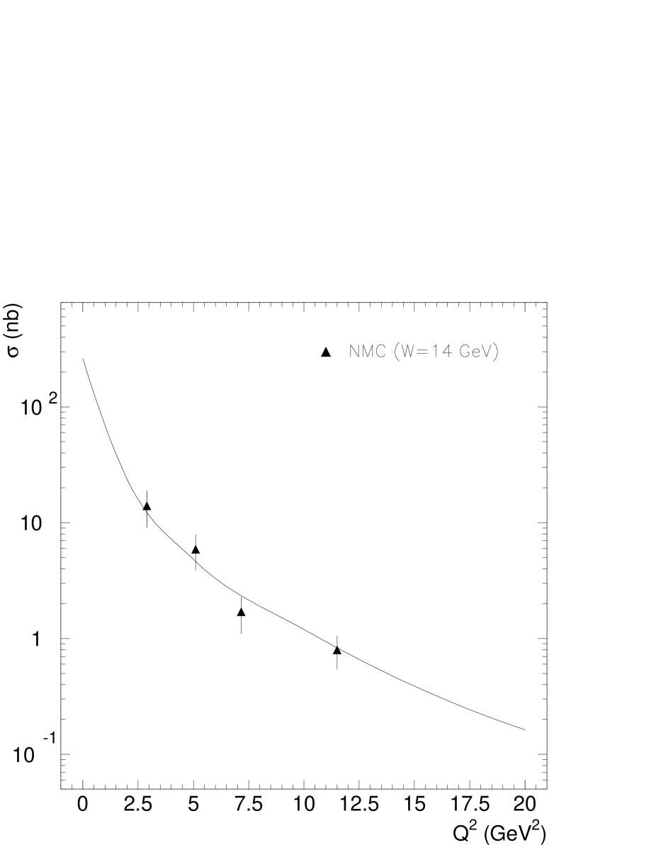
Figure 20: $Q^{2}$ dependence of the $\phi$ -meson cross-section at $W=14\,{\rm Ge}\kern-1.0pt{\rm V}$ in model S2. The data are from NMC [48].

The results for the $\phi$ with $p_{F}=0.6$ GeV are shown in figures 17, 17 and 18 for S1 and in figures 20, 20 and 21 for S2. The results in both cases are very good. It is particularly satisfying that the description of the low-energy data is good, as in this case there is no reggeon contribution. Once again the results obtained using the wave functions derived from the specific potentials are very close to those shown, and provide an equally good description.

The $J\!/\!\Psi$ results are given in figures 23 through 27 with $p_{F}=1.2$, and are again very satisfactory. We have included low-energy data, although they are not very precise and have some contamination from nucleon breakup. Because of the mass of the charm quark the data on $\sigma_{L}/\sigma_{T}$ ratio do not provide a strong constraint, and even at $Q^{2}=50$ GeV² the ratio is still far from its asymptotic value. The S2 results are again to be slightly preferred overall. In the case of the $J\!/\!\Psi$ the results obtained using the wave functions derived from the specific potentials do not provide a good description of the data, the cross section being about a factor of three too large. There are also significant differences in $\sigma_{L}/\sigma_{T}$, the ratio rising almost linearly with increasing $Q^{2}$, and by $Q^{2}=50$ GeV² is a factor of two larger than the results shown in figures 24 and 27. However the present data cannot sensibly distinguish between this result and the one shown. That there is a significant difference in the predictions for the $J\!/\!\Psi$ is not surprising given the very different wave function used in the fit compared to those obtained from specific potentials: recall figure 9.

There is very little difference in the energy dependence predicted by models S1 and S2, so we shall show only the latter. The energy dependence at fixed $Q^{2}$ is shown in figures 29 and 29 for the $\rho$, in figure 31 for the $\phi$ and in figure 31 for the $J/\psi$, in each case for the S2 model. The break in the curves is because of the different value of $\epsilon$ used at the lower energies. The model succeeds well in reproducing the trends of the data, and is particularly successsful for the $\phi$ and $J/\psi$, even at $Q^{2}=0$ in the latter case. The increasing energy dependence with increasing $Q^{2}$ is well represented by the model, reflecting the increasing importance of the hard pomeron as $Q^{2}$ is increased. This is not artifically imposed on the model. It occurs naturally via the loop integrals involving the meson wave function and the gluon propagators. The model also automatically takes account of the increasing importance of the hard pomeron with increasing quark mass. For example, for the $\rho$ at $Q^{2}=0$ the soft pomeron contributes $95\%$ of the amplitude at $\sqrt{s}=15$ GeV and $85\%$ of the amplitude at $\sqrt{s}=75$ GeV. At $Q^{2}=20$ GeV² these have become $25\%$ of the amplitude at $\sqrt{s}=15$ GeV and $10\%$ of the amplitude at $\sqrt{s}=75$ GeV. These proportions are very similar for the $\phi$  with a slight increase of the hard component: for example at $Q^{2}=0$ the soft pomeron contributes $90\%$ of the amplitude at $\sqrt{s}=15$ GeV and $70\%$ of the ampitude at $\sqrt{s}=90$ GeV. For the $J\!/\!\Psi$ at $Q^{2}=0$ the soft pomeron contributes $80\%$ of the amplitude at $\sqrt{s}=15$ GeV and $35\%$ at $\sqrt{s}=250$ GeV. These results for the soft pomeron proportions at $Q^{2}=0$ are comparable with those obtained in other phenomenological approaches [8, 41]. The same general features, a slow onset of the perturbative region where the hard pomeron dominates, are compatible with those of [68, 69]. In [68] a theoretical analysis is made of $\gamma^{*}p\rightarrow\rho^{0}p$ based on the BFKL formalism, and it is concluded that the perturbative term does not dominate until energies and virtualities beyond those currently accessed at HERA. In [69] an analysis of $J/\psi$ photoproduction in a dipole model clearly illustrates the mixing of perturbative and nonperturbative effects in this process.

Finally, examples of the predicted $t$-dependence are shown in figures 33 to 35. The data for the $\rho$ and $\phi$ are unnormalised, so the theoretical curves have been renormalized to the data. The relative normalisation of S1 and S2 is that given by the models. For the $J\!/\!\Psi$ the data and the predictions are normalised. Clearly the description is again very satisfactory, with the possible exception of the $\rho$  where the models predict a somewhat faster decrease with $t$ than is observed.

6 Conclusions

We have presented a model of vector meson electroproduction, and also for photoproduction in the case of the $J\!/\!\Psi$. The model gives a good overall description of the data for $\rho$, $\phi$ and $J/\psi$ electroproduction with only five adjustable parameters. The dynamical mechanism, with two adjustable parameters, is common to each and the only freedom in going from one vector meson to another is the parameter $p_{F}$ which is related to the “size” of the meson in its rest frame. The values of $p_{F}$ required for each of the $\rho$, $\phi$ and $J/\psi$ are 0.5 GeV², 0.6 GeV² and 1.2 GeV² respectively, in accord with what one would expect. Not surprisingly, electroproduction of the $\rho$ is primarily non-perturbative at small $Q^{2}$, and an important non-perturbative component is still present at the highest energy and largest $Q^{2}$ for which data exist. In contrast the perturbative contribution dominates in $J/\psi$ production at high energy, although at small $Q^{2}$ interference with the non-perturbative contribution remains important. For $W\geq 50$ GeV, $Q^{2}\geq 20$ GeV² $J\!/\!\Psi$ electroproduction can be considered to be exclusively perturbative. We finally note that this type of model could be used to give an excellent description of any of the $\rho$, $\phi$ and $J/\psi$ if they were to be considered in isolation.

Figure 10: $Q^{2}$ dependence of the $\rho$ -meson cross-section at $W=75\,{\rm Ge}\kern-1.0pt{\rm V}$ in model S1.The data are from: H1 [64]; and ZEUS [51] [60] [62].

Figure 11: $Q^{2}$ dependence of the $\rho$ -meson cross-section at $W=15\,{\rm Ge}\kern-1.0pt{\rm V}$ in model S1. The data are from: NMC [48].

Figure 12: $Q^{2}$ dependence of the $\rho$ -meson  longtitudinal to transverse cross-section ratio at $W=75\,{\rm Ge}\kern-1.0pt{\rm V}$ in model S1. The data are from: CHIO [42]; NMC [48]; E665 [57]; H1 [52] [53] [64]; and ZEUS [49] [51] [62].

Figure 13: $Q^{2}$ dependence of the $\rho$ -meson cross-section at $W=75\,{\rm Ge}\kern-1.0pt{\rm V}$ in model S2. The data are from: H1 [64]; and ZEUS [51] [60] [62].

Figure 14: $Q^{2}$ dependence of the $\rho$ -meson cross-section at $W=15\,{\rm Ge}\kern-1.0pt{\rm V}$ in model S2. The data are from: NMC [48].

Figure 15: $Q^{2}$ dependence of the $\rho$ -meson  longtitudinal to transverse cross-section ratio at $W=75\,{\rm Ge}\kern-1.0pt{\rm V}$ in model S2. The data are from: CHIO [42]; NMC [48]; E665 [57]; H1 [52] [53] [64]; and ZEUS [49] [51] [62].

Figure 16: $Q^{2}$ dependence of the $\phi$ -meson cross-section at $W=90\,{\rm Ge}\kern-1.0pt{\rm V}$ in model S1. The data are from: H1 [59] [67]; and ZEUS [55]  [56] [61].

Figure 17: $Q^{2}$ dependence of the $\phi$ -meson cross-section at $W=14\,{\rm Ge}\kern-1.0pt{\rm V}$ in model S1. The data are from NMC [48].

Figure 18: $Q^{2}$ dependence of the $\phi$ -meson  longtitudinal to transverse cross-section ratio at $W=90\,{\rm Ge}\kern-1.0pt{\rm V}$ in model S1. The data are from: H1 [67]; and ZEUS [61].

Figure 19: $Q^{2}$ dependence of the $\phi$ -meson cross-section at $W=90\,{\rm Ge}\kern-1.0pt{\rm V}$ in model S2. The data are from: H1 [59] [67]; and ZEUS [55]  [56] [61].

Figure 21: $Q^{2}$ dependence of the $\phi$ -meson  longtitudinal to transverse cross-section ratio at $W=90\,{\rm Ge}\kern-1.0pt{\rm V}$ in model S2. The data are from: H1 [67]; and ZEUS [61].

Figure 22: $Q^{2}$ dependence of the $J\!/\!\Psi$ -meson cross-section at $W=90\,{\rm Ge}\kern-1.0pt{\rm V}$ in model S1. The data are from H1 [54] [63]; and ZEUS [58] [62].

Figure 23: $Q^{2}$ dependence of the $J\!/\!\Psi$ -meson cross-section at $W=14\,{\rm Ge}\kern-1.0pt{\rm V}$ in model S1. The data are from EMC [44]; E401 [43]; E516 [45]; NA14 [46]; and E687 [47].

Figure 24: $Q^{2}$ dependence of the $J\!/\!\Psi$ -meson  longtitudinal to transverse cross-section ratio at $W=90\,{\rm Ge}\kern-1.0pt{\rm V}$ in model S1. The data are from: H1 [54] [63]; and ZEUS [58] [62].

Figure 25: $Q^{2}$ dependence of the $J\!/\!\Psi$ -meson cross-section at $W=90\,{\rm Ge}\kern-1.0pt{\rm V}$ in model S2. The data are from H1 [54] [63]; and ZEUS [58] [62].

Figure 26: $Q^{2}$ dependence of the $J\!/\!\Psi$ -meson cross-section at $W=14\,{\rm Ge}\kern-1.0pt{\rm V}$ in model S2. The data are from The data are from EMC [44]; E401 [43]; E516 [45]; NA14 [46]; and E687 [47].

Figure 27: $Q^{2}$ dependence of the $J\!/\!\Psi$ -meson  longtitudinal to transverse cross-section ratio at $W=90\,{\rm Ge}\kern-1.0pt{\rm V}$ in model S2. The data are from: H1 [54] [63]; and ZEUS [58] [62].

Figure 28: $W$ dependence of the $\rho$ -meson cross-section for various $Q^{2}$ in model S2. The data are from: NMC [48]; H1 [64]; and ZEUS [62].

Figure 29: $W$ dependence of the $\rho$ -meson cross-section for various $Q^{2}$ in model S2. The data are from H1 [64].

Figure 30: $W$ dependence of the $\phi$ -meson cross-section for various $Q^{2}$ in model S2. The data are from: NMC [48]; H1 [59]; and ZEUS [55]  [56] [61].

Figure 31: $W$ dependence of the $J\!/\!\Psi$ meson cross-section for various $Q^{2}$ in model S2. The data are from: EMC [44]; E401 [43]; E516 [45]; NA14 [46]; E687 [47]; H1 [54] [66]; and ZEUS [50] [58].

Figure 32: $\rho$ meson $t$ dependence, $\langle Q^{2}\rangle=4.8$ GeV², $30<W<140$ GeV. The dashed line is for the S1 model, the dotted line for the S2 model. The overall normalisation is arbitrary, but the relative normalisation of the S1 and S2 predictions are as given by the model. The data are from H1 [64].

Figure 33: $\rho$ meson $t$ dependence, $\langle Q^{2}\rangle=10.9$ GeV², $30<W<140$ GeV. The dashed line is for the S1 model, the dotted line for the S2 model. The overall normalisation is arbitrary, but the relative normalisation of the S1 and S2 predictions are as given by the model. The data are from H1 [64].

Figure 34: $\phi$ meson $t$ dependence, $\langle Q^{2}\rangle=4.5$ GeV², $40<W<130$ GeV. The dashed line is for the S1 model, the dotted line for the S2 model. The overall normalisation is arbitrary, but the relative normalisation of the S1 and S2 predictions are as given by the model. The data are from H1 [67].

Figure 35: $J/\psi$ meson $t$ dependence, $Q^{2}=0$, $91<W<110$ GeV. The dashed line is for the S1 model, the dotted line for the S2 model. The data are from: H1 [66]; and ZEUS [65].

References

- [1] J C Collins, L Frankfurt and M Strikman: Phys.Rev. D56 (1997) 2982
- [2] A Hebecker and P V Landshoff: Phys.Lett. B419 (1998) 393
- [3] M Diehl, Z.Phys. C66 (1995) 181
- [4] I Royen and J R Cudell: Nucl.Phys. B545 (1999) 505
- [5] A Donnachie, J Gravelis and G Shaw: hep-ph/0009235; Eur.J.Phys. C (in press)
- [6] P Moseley and G Shaw: Phys.Rev. D52 (1995) 4941; G Kerley and G Shaw: Phys.Rev. D56 (1997) 7291
- [7] A Donnachie and P V Landshoff: Phys.Lett. B437 (1998) 408
- [8] A Donnachie and P V Landshoff: Phys. Lett. B478 (2000) 146
- [9] J R Forshaw, G Kerley and G Shaw: Phys.Rev. D60 (1999) 074012; Nucl.Phys. A675 (2000) 80; and hep-ph/0007257.
- [10] J Kwiecinski and L Motyka: Phys.Lett. B462 (1999) 203
- [11] A Donnachie, H G Dosch and M Rueter: Phys.Rev. D59 (1999) 074011; Eur.Phys.J. C13 (2000) 141
- [12] E Gotsman, E Levin, U Maor and E Naftali: Eur.Phys.J. C10 (1999) 689; Eur.Phys.J. C14 (2000) 511
- [13] E M Levin, A D Martin, M G Ryskin and T Teubner: Z.Phys. C74 (1997) 671; A D Martin, M G Ryskin and T Teubner: Phys. Rev. D55 (1997) 4329
- [14] S J Brodsky and G P Lepage: Phys.Rev. D22 (1980) 2157
- [15] J Gravelis: Exclusive Vector Meson Electroproduction, PhD Thesis (Manchester, 2000).
- [16] P V Landshoff and O Nachtmann: Z.Phys. C35 (1987) 405
- [17] A Donnachie and P V Landshoff: Nucl.Phys. B311 (1988/89) 509
- [18] A Donnachie and P V Landshoff: Nucl.Phys. B267 (1986) 690
- [19] J R Cudell and B U Nguyen: Nucl. Phys. B420 (1994) 669
- [20] J R Cudell and I Royen: Phys.Lett. B397 (1997) 317
- [21] H Plothow-Besch: PDFLIB: Nucleon, Pion and Photon Parton Density Functions and Calculations. Users’ Manual. Version 7.09, CERN, 1997
- [22] H L Lai et al.: Phys.Rev. D55 (1997) 1280
- [23] A Donnachie and P V Landshoff: Phys.Lett. B470 (1999) 243
- [24] I Halperin and A Zhitnitsky: Phys.Rev. D56 (1997) 184
- [25] F Schlumpf: Phys.Rev. D50 (1994) 6895
- [26] Tao Huang, Bo-Qiang Ma and Qi-Xing Shen, Phys.Rev. D49 (1994) 1490
- [27] B Chibisov and A Zhitnitsky: Phys.Rev. D52 (1995) 5273
- [28] A F Krutov and V E Troitsky: hep-ph/9707534.
- [29] J P B C de Melo, T Frederico, L Tomio and A E Dorokhov: Nucl.Phys. A623 (1997) 456
- [30] V M Belyaev and M B Johnson: Phys.Lett. B423 (1998) 379
- [31] E J Eichten and C Quigg: Phys.Rev. D52 (1995) 1726
- [32] A Martin: Phys.Lett. B93 (1980) 338
- [33] C Quigg and J L Rosner: Phys.Lett. B71 (1977) 153; Phys.Rep. 56 (1979) 167.
- [34] E Eichen, K Gottfried, T Kinoshita, K D Lane and T-M Yan: Phys.Rev. D17 (1978) 3090; Phys.Rev. D21 (1980) 203
- [35] W Buchmüller and S-H H Tye: Phys.Rev. D24 (1981) 132
- [36] L Frankfurt, W Koepf and M Strikman: Phys.Rev. D57 (1998) 512
- [37] J Nemchik, N N Nikolaev, E Predazzi and B G Zakharov: Z.Phys. C75 (1997) 71
- [38] A Donnachie and P V Landshoff: Phys.Lett. B185 (1987) 403
- [39] R R Horgan, P V Landshoff and D M Scott, Phys.Lett. 110B (1982) 493.
- [40] H G Dosch, T Gousset and H J Pirner: Phys.Rev. D57 (1998) 1666
- [41] P Gauron and B Nicolescu: Phys.Lett. B486 (2000) 71
- [42] W D Shambroom et al (CHIO Collaboration): Phys.Rev. D26 (1982) 1
- [43] M Binkley et al (E401 Collaboration): Phys.Rev.Lett. 48 (1982) 73
- [44] J J Aubert et al (EMC Collaboration): Nucl.Phys. B213 (1983) 1
- [45] B H Denby et al (E516 Collaboration): Phys.Rev.Lett. 52 (1984) 795
- [46] R Barate et al (NA14 Collaboration): Z.Phys. C33 (1987) 505
- [47] P L Frabetti et al (E687 Collaboration): Phys.Lett. B316 (1993) 197
- [48] M Arneodo et al (NMC Collaboration): Nucl.Phys. B429 (1994) 503
- [49] M Derrick et al (ZEUS Collaboration): Z.Phys. C69 (1995) 39
- [50] M Derrick et al (ZEUS Collaboration): Phys.Lett. B350 (1995) 120
- [51] M Derrick et al (ZEUS Collaboration): Phys.Lett. B356 (1995) 601
- [52] S Aid et al (H1 Collaboration): Nucl.Phys. B463 (1996) 3
- [53] S Aid et al (H1 Collaboration): Nucl.Phys. B468 (1996) 3
- [54] S Aid et al (H1 Collaboration): Nucl.Phys. B472 (1996) 32
- [55] M Derrick et al (ZEUS Collaboration): Phys.Lett. B377 (1996) 259
- [56] M Derrick et al (ZEUS Collaboration): Phys.Lett. B380 (1996) 220
- [57] M R Adams et al (E665 Collaboration): Z.Phys. C74 (1997) 237
- [58] J Breitweg et al (ZEUS Collaboration): Z.Phys. 75 (1997) 215
- [59] C Adloff et al (H1 Collaboration): Z.Phys. C75 (1997) 607
- [60] J Breitweg et al (ZEUS Collaboration): Eur.Phys.J. C2 (1998) 247
- [61] ZEUS Collaboration: submitted paper 793 to ICHEP 1998
- [62] J Breitweg et al (ZEUS Collaboration): Eur.Phys.J C6 (1999) 603
- [63] C Adloff et al (H1 Collaboration): Eur.Phys.J. C10 (1999) 373
- [64] C Adloff et al (H1 Collaboration): Eur.Phys.J. C13 (2000) 371
- [65] J Breitweg et al (ZEUS Collaboration): Eur.Phys.J C14 2000) 213
- [66] C Adloff et al (H1 Collaboration): Phys.Lett. B483 2000) 23
- [67] C Adloff et al (H1 Collaboration): Phys.Lett. B483 (2000) 360
- [68] V V Anisovich et al: Phys.Rev. D60 (1999) 074011
- [69] L Frankfurt, M McDermott and M Strikman: hep-ph/0009086