hep-ph/0101210

SNS-PH/01-01

Relic Dark Energy from Trans-Planckian Regime

Laura Mersini, Mar Bastero-Gil and Panagiota Kanti

Scuola Normale Superiore and INFN, Piazza dei Cavalieri 7,
I-56126 Pisa, Italy

As yet, there is no underlying fundamental theory for the transplanckian regime. There is a need to address the issue of how the observables in our present Universe are affected by processes that may have occurred at superplanckian energies (referred to as the transplanckian regime). Specifically, we focus on the impact the transplanckian regime has on two observables, namely: dark energy and the CMBR spectrum. We model the transplanckian regime by introducing a 1-parameter family of smooth non-linear dispersion relations which modify the frequencies at very short distances. A particular feature of the family of dispersion functions chosen is the production of ultralow frequencies at very high momenta $k$ (for $k>M_{P}$). We name the range of the ultralow energy modes (of very short distances) that have frequencies equal or less than the current Hubble rate $H_{0}$ as the tail modes. These modes are still frozen today due to the expansion of the Universe. We calculate their energy today and show that the $tail$ provides a strong candidate for the dark energy of the Universe. During inflation, their energy is about 122-123 orders of magnitude smaller than the total energy, for any random value of the free parameter in the family of dispersion relations. For this family of dispersions, we present the exact solutions and show that: the CMBR spectrum is that of a (nearly) black body, and that the adiabatic vacuum is the only choice for the initial conditions.

Emails: mersini@cibs.sns.it, bastero@cibs.sns.it, kanti@cibs.sns.it

1 Introduction

There is still no fundamental physical theory of the very early universe which addresses issues that arise from the regime of transplanckian physics. One of these issues relates to the origin of the cosmological perturbation spectrum. In an expanding Universe, the physical momentum gets blue-shifted back in time, therefore the observed low values of the momentum today that contribute to the CMBR spectrum may have originated from values larger than the Planck mass $M_{P}$ in the Early Universe. This is similar to the problems that arise in trying to explain the origin of Hawking radiation in Black Hole physics. In a series of papers [1, 2, 3, 4, 5], it was demonstrated that the Hawking radiation remains unaffected by modifications of the ultra high energy regime, expressed through the modification of the usual linear dispersion relation at energies larger than a certain ultraviolet scale $k_{C}$. Following a similar procedure, in the case of an expanding Friedmann-Lemaitre-Robertson-Walker (FLRW) spacetime, Martin and Brandenberger in Ref. [6] (see also [7, 8, 9, 10, 11]) showed that standard predictions of inflation are indeed sensitive to trans-planckian physics: different dispersion relations lead to different results for the CMBR spectrum.

It is the lack of a fundamental theory, valid at all energies, that makes the model building of the transplanckian regime very interesting. The main issue is how much are the known observables affected by the unknown theory. The apparently ad hoc modification of the dispersion relation at high energies is contrained by the criterion that its low energy predictions do no conflict the observables. Specifically, in this paper we address two questions: a) can the transplanckian regime contribute to the dark energy of the universe, and b) how sensitive is the CMBR spectrum to energies higher than the Planck scale $M_{P}$, where our current physics theory is known to break down.

We choose a family of dispersion relations for the frequency of the wavefunctions that modifies the behaviour of the field at the ultrahigh energies of the transplanckian regime. The dispersion relation has the following features: it is smooth, nearly linear for energies less than the Planck scale, reaches a maximum, and attenuates to zero at ultrahigh momenta thereby producing ultralow frequencies at very short distances. We name the $tail$ that part of the dispersion graph of very short distances that contains the range of ultralow frequencies less or equal to the current Hubble constant $H_{0}$. It follows that the $tail$ modes are still currently frozen. We calculate the energy of the $tail$ modes in order to address the former question (a) and show that although the $tail$ does not contribute significantly to the CMBR spectrum, it has a dominant contribution to the dark energy of the universe [12]. The energy density of the $tail$ modes is of the same order today as the matter energy density.

The second question (b) is motivated by the problem that in most inflationary models the present large scale structure of the Universe is extrapolated from a regime of ultra-high energies (known as the transplanckian regime) originating from before the last 60 e-foldings of the exponential expansion. In Refs. [6, 8] the authors have demonstrated that the problem of calculating the spectrum of perturbations with a time-dependent dispersive frequency can be reduced to the familiar topic of particle creation on a time-dependent background [13]. We will use their observation in what follows. They also conjecture that the observed power spectrum can always be recovered only by using a smooth dispersion relation, which ensures an adiabatic time-evolution of the modes. By taking the frequency dispersion relations to be the general class of Epstein functions [14], we check and lend strong support to their conjecture. We present the exact solutions to the mode equation for the scalar field with a “time-dependent mass”, and the resulting CMBR spectrum below. We show that the major contribution to the CMBR spectrum comes from the long wavelength modes when they re-enter the horizon. The spectrum is nearly insensitive to the very short wavelength modes inside the Hubble horizon.

The paper is organized as follows: in Section 2, we present the set-up and formalism of our analysis. The family of dispersion functions, exact solutions to the mode equations of motion and the resulting CMBR spectrum (from the Bogoliubov method) are reported in Section 3. In Section 4, we calculate the contribution of the tail modes to the dark energy of the universe today. In this work, we have neglected the backreaction effects of particle production. This assumption is fully justified from the calculation of the energy for the transplanckian modes, in Section 4. Due to the dispersed ultralow frequency of these modes, the energy contained in that transplanckian regime is very small ($10^{-122}\rho_{total}$), thus the backreaction effect is reasonably negligible [15, 6]. We present our conclusions in Section 5.

2 The Set-Up and Formalism

Let us start with the generalized Friedmann-Lemaitre-Robertson-Walker (FLRW) line-element which, in the presence of scalar and tensor perturbations, takes the form [17, 18]

$$ds^{2} = a^{2}(\eta)\left\{-d\eta^{2}+\left[\delta_{ij}+h(\eta,{\bf n})Q\delta_{ij}\right.\right.$$ (1)

$$\left.\left.+h_{l}(\eta,{\bf n})\frac{Q_{ij}}{n^{2}}+h_{gw}(\eta,{\bf n})Q_{ij}\right]dx^{i}dx^{j}\right\}\,,$$

where $\eta$ is the conformal time and $a(\eta)$ the scale factor. The dimensionless quantity ${\bf n}$ is the comoving wavevector, related to the physical vector ${\bf k}$ by ${\bf k}={\bf n}/a(\eta)$ as usual. The functions $h$ and $h_{l}$ represent the scalar sector of perturbations while $h_{gw}$ represents the gravitational waves. $Q(x^{i})$ and $Q_{ij}(x^{i})$ are the eigenfunction and eigentensor, respectively, of the Laplace operator on the flat spacelike hypersurfaces. For simplicity, we will take a scale factor $a(\eta)$ given by a power law, $a(\eta)=|\eta_{c}/\eta|^{\beta}$, where $\beta\geq 1$ and $|\eta_{c}|=\beta/H(\eta_{c})$. The initial power spectrum of the perturbations can be computed once we solve the time-dependent equations in the scalar and tensor sector. The mode equations for both sectors reduce [19, 20, 21] to a Klein-Gordon equation of the form

$$\mu_{n}^{\prime\prime}+\left[n^{2}-\frac{a^{\prime\prime}}{a}\right]\mu_{n}=0\,,$$ (2)

where the prime denotes derivative with respect to conformal time. Therefore, studying perturbations in a FLRW background is equivalent to solving the mode equations for a scalar field $\mu$ related (through Bardeen variables [21]) to the perturbation field in the expanding background. The above equation represents a linear dispersion relation for the frequency $\omega$,

$$\omega^{2}=k^{2}=\frac{n^{2}}{a^{2}}\,.$$ (3)

The dispersion relation of Eq. (3) holds for values of momentum smaller than the Planck scale. There is no reason to believe that it remains linear at ultra-high energies larger than $M_{P}$. Yet, nonlinear dispersion relations are quite likely to occur from the Lagrangian of some effective theory obtained by the yet unknown fundamental theory. Nonlinear dispersion relations, similar to the ones we consider in this work, are known to arise in effective theories of: nonlocal condensed matter or particle physics models arising from non-canonical kinetic terms [22, 23]; from the dissipative behavior of a quantum system immersed into an environment after coarse-graining [24]; or from effective theories with phase transitions, time-dependent mass squared terms or effective potentials [25, 26, 27]. Perhaps, trans-planckian models motivated by superstring theory [28, 29] or a two-stage inflationary model [30] are plausible. In the latter case, one could easily envision for example a scenario with the first stage of inflation occurring at energy scales above the Planck mass  followed by a nonthermal phase transition [31]. The preheating [31, 32] from the nonthermal phase transition then leads to the second stage of inflation below Planck energies. In the former case, the motivation comes from the common belief that the superstring theory is the one that describes or at least is valid at energies of the transplanckian period. Taking this idea one step further, we incorporate the concept of superstring duality (which applies at transplanckian regimes) in our analysis by choosing a particular family of dispersion relations that exhibits dual behavior, i.e. appearance of ultra-low mode frequencies both at low and high momenta $k$.

Despite the above comments and possible approaches, we should stress that any modeling of Planck scale physics by analogy with the already familiar systems is pure speculation. We lack the fundamental theory that may naturally motivate or reproduce such dispersion behaviour. Nevertheless, it would be instructive to derive these dispersion relations from particle physics and string theory, as a step towards understanding the physical nature of the model.

In what follows, we replace the linear relation $\omega^{2}(k)=k^{2}=n^{2}/a(\eta)^{2}$ with a nonlinear dispersion relation $\omega(k)=F(k)$. The family of dispersion functions $F(k)$ for our model is introduced in section 3. These functions have the following features: they are linear for low momenta up to the Plank scale $k_{C}=M_{P}$, taken to be the cuttoff scale, but beyond the cutoff they smoothly turn down and asymptotically approach zero whereby producing ultra-low frequencies at very short distances. Therefore, in Eq. (2), $n^{2}$ should be replaced by:

$$n_{eff}^{2}=a(\eta)^{2}F(k)^{2}=a(\eta)^{2}F[n/a(\eta)]^{2}\,.$$ (4)

We will also consider the general case of non-minimal or conformal coupling to gravity by keeping some arbitrary, unspecified, coupling constant $\xi$. Then, the equation for the scalar and tensor perturbations, that we need to solve, takes the form

$$\mu_{n}^{\prime\prime}+\left[n^{2}_{eff}-(1-6\xi)\frac{a^{\prime\prime}}{a}\right]\mu_{n}=0\,.$$ (5)

For future reference, we define the generalised comoving frequency as

$$\Omega_{n}^{2}=n^{2}_{eff}-(1-6\xi)\frac{a^{\prime\prime}}{a}\,.$$ (6)

The dynamics of the scale factor is determined by the evolution of the background inflaton field $\phi$, with potential $V(\phi)$, and the Friedmann equation. In conformal time, these equations are:

$$\frac{a^{\prime\prime}}{a}-\frac{a^{\prime^{2}}}{a^{2}}+\frac{8\pi G}{3}\left(\phi^{\prime^{2}}-a^{2}V(\phi)\right) = 0\,,$$ (7)

$$\phi^{\prime\prime}+2\frac{a^{\prime}}{a}\phi^{\prime}+a^{2}\frac{\partial V(\phi)}{\partial\phi} = 0\,.$$ (8)

Most of the contribution in the perturbation spectrum comes from long-wavelength modes, since at late times they are non relativistic and act like a classical homogeneous field with an amplitude $\bar{\mu}$ given by:

$$\bar{\mu}=\sqrt{\langle\mu^{2}\rangle}=\left(\frac{1}{2\pi a^{3}}\int dn\,n^{2}\,|\mu_{n}|^{2}\right)^{1/2}\,.$$ (9)

These are produced at early stages of inflation, thus they are very sensitive to the initial conditions. The correct vacuum state is given by the solution to Eq. (5) as clarified below. But if the stage of inflation is very long, and the Hubble parameter $H$ is not changing considerably, then a Minkowski-like vacuum is a good first order approximation for the initial vacuum state ($\eta\rightarrow-\infty$), with:

$$\mu_{n}(\eta)\simeq\frac{1}{\sqrt{2n}}e^{-in\eta}\,.$$ (10)

However, if $H$ was greater at the early stages of inflation, before the last 60 e-foldings, and/or the inflationary stage is short, then one must solve the wave equation and find the solution that minimizes the energy [33, 34, 27]. This is the correct vacuum state of the system. Otherwise, if one a priori chooses the Minkowski vacuum to be the initial vacuum state describing the system, the resulting value of $\langle\mu^{2}\rangle$ is considerably underestimated as shown rigorously by Felder et al. [35].

As already shown in Ref. [6], Eq. (5) represents particle production in a time-dependent background. We will follow the method of Bogoliubov transformation to determine the spectrum. The correct initial condition for the vacuum state is the solution to the equation that minimizes the energy. Hence, if the ’time-dependent’ background goes asymptotically flat at late times, then in that limit the wavefunction should behave as a plane wave:

$$\mu_{n}\rightarrow_{\eta\rightarrow-\infty}\frac{1}{\sqrt{\Omega_{n}^{in}}}e^{-i\Omega^{in}_{n}\eta}\,.$$ (11)

As it is well known on this scenario, in general at late times one has a squeezed state due to the curved background that mixes positive and negative frequencies. The evolution of the mode function $\mu_{n}$ at late times fixes the Bogoliubov coefficients $\alpha_{n}$ and $\beta_{n}$,

$$\mu_{n}\rightarrow_{\eta\rightarrow+\infty}\frac{\alpha_{n}}{\sqrt{2\Omega^{out}_{n}}}e^{-i\Omega^{out}_{n}\eta}+\frac{\beta_{n}}{\sqrt{2\Omega^{out}_{n}}}e^{+i\Omega^{out}_{n}\eta}\,.$$ (12)

with the normalization condition:

$$|\alpha_{n}|^{2}-|\beta_{n}|^{2}=1\,.$$ (13)

In the above expressions, $\Omega^{in}_{n}$ and $\Omega^{out}_{n}$ denote the asymptotic values of $\Omega_{n}$ when $\eta\rightarrow\mp\infty$. The spectrum of particles per mode is then calculated with the conventional Bogoliubov method [34]. The number of particles created $n$ and their energy density $\rho$ are calculated by the following expressions

$$\langle n\rangle = \frac{1}{2\pi^{2}a^{3}}\int dn~{}n^{2}|\beta_{n}|^{2}\,,$$ (14)

$$\langle\rho\rangle = \frac{1}{2\pi^{2}a^{4}}\int ndn\int n_{eff}dn_{eff}~{}|\beta_{n}|^{2}$$ (15)

$$= \frac{1}{2\pi^{2}}\int kdk\int\omega(k)d\omega~{}|\beta_{k}|^{2}\,.$$

If the resulting Bogoliubov coefficient $\beta_{k}$ of the particles produced has a (nearly) thermal distribution, we can conclude that the CMBR in our problem is that of a (nearly) black body spectrum. We introduce the class of Epstein functions as the family of dispersion relations in Section 3, and derive the CMBR spectrum from the exact solutions to the evolution equations.

Meanwhile, for the special features of our choice of dispersion relation, the modes at very high momenta but of ultra low frequencies $\omega(k)$ are frozen for as long as the Hubble expansion rate $H$ of the Universe dominates over their frequency. We refer to that as the $tail$ of the dispersion graph. In Fig. (2), for the dispersed $\omega^{2}(k)$ vs. $k$, the tail corresponds to all the modes beyond the point $k_{H}$, where $k_{H}$ is defined by the condition $\omega^{2}(k_{H})=H^{2}_{0}$, where $H_{0}$ is the Hubble rate today. It then follows that the tail modes are still frozen at present. We calculate the total energy of the particles by using Eq. (15), as well as the frozen energy of the $tail$. Thus the energy of the tail is a contribution to the dark energy of the universe: up to present it has the equation of state of a cosmological constant term. However, through the Friedmann equation, $H$ is a decreasing function of time because until now it has been dominated by the energy density of matter and radiation. Therefore, whenever $H$ drops below the frequency $\omega$ of an ultralow frequency mode, this mode becomes dynamic by picking a kinetic term and redshifts away very quickly. Hence, when the dominant contribution to the evolution equation for $H$ comes from the $tail$ energy, the behaviour of those modes with equations of motion coupled to the Friedmann equation becomes very complex. It is hard to calculate at which rate $H$ drops in this situation. If eventually, $H$ drops all the way to zero, all the modes in the tail must have decayed. Their equation of state, when $H$ becomes zero, is that of radiation. The reason can be traced back at their origin in transplanckian regime. It is well known that scalar perturbations produced during inflation do not contribute to the total energy. Thus the origin of this modes is in the tensor perturbations. In their physical nature they correspond to gravitational waves of very short distance but ultralow energy. We calculate their energy today in Section 4.

We would like to elaborate on yet another possibility, which has not been mentioned before in the literature, that can give rise to a similar dispersion relation: very short or very large distance physics may have a curvature different from the FLRW element of Eq. (1), e.g. a different scale factor. This becomes clearer when recognizing the strong relation between the time-dependent dispersion relation and the curvature given by the time derivatives of the scale factor $a(\eta)$. The basic argument is the observation that the modulated frequency $\Omega_{n}^{2}$ in the wave equation contains the contribution of these two terms, as given in Eq. (6). Therefore, while keeping the generalised frequency invariant, changing the first term in $\Omega_{n}^{2}$ can be viewed or attributed to changes in the second term, such that:

$$\Omega_{n}^{2}=a^{2}\omega_{nonlinear,k}^{2}-(1-6\xi)\,\frac{a^{\prime\prime}}{a}={\mathcal{A}}^{2}\omega_{linear,k}^{2}-(1-6\xi)\,\frac{\mathcal{A}^{\prime\prime}}{\mathcal{A}}\,,$$ (16)

where $\mathcal{A}$ is the new scale factor at very short distances. Even in the conformal case $\xi=1/6$, when the term $a^{\prime\prime}/a$ drops out of Eq. (5), the time dependent frequency $\omega_{nonlinear,k}^{2}$ can mimic a term proportional to $a^{\prime\prime}/a$ at $\lambda(\eta)k_{C}\ll 1$. Thus, any modulation of the dispersion relation is equivalent to a change in the behavior of the time-dependence of the background (a.k.a., the scale factor/curvature). In other words, we could have introduced a different curvature at very short (or large) distances from the start instead of a dispersed frequency.

3 Exact Solution and the CMBR Spectrum

We will consider the class of inflationary scenarios that through Eqs. (7) and (8) has a power law solution for the scale factor $a(\eta)$ in conformal time, $a(\eta)=|\eta_{c}/\eta|^{\beta}$, with $\beta\geq 1$, and the following Epstein function [14] for the dispersion relation:

$$\omega^{2}(k) = F^{2}(k)=k^{2}\left(\frac{\epsilon_{1}}{1+e^{x}}+\frac{\epsilon_{2}e^{x}}{1+e^{x}}+\frac{\epsilon_{3}e^{x}}{(1+e^{x})^{2}}\right)\,,$$ (17)

$$n^{2}_{eff} = a^{2}(\eta)F^{2}(n,\eta)=n^{2}\left(\frac{\epsilon_{1}}{1+e^{x}}+\frac{\epsilon_{2}e^{x}}{1+e^{x}}+\frac{\epsilon_{3}e^{x}}{(1+e^{x})^{2}}\right)\,,$$ (18)

where $x=(k/k_{C})^{1/\beta}=A|\eta|$, with $A=(1/|\eta_{c}|)(n/k_{C})^{1/\beta}$. This is the most general expression for this family of functions. For our purposes, we will constrain some of the parameters of the Epstein family in order to satisfy the features required for the dispersion relation as follows. First, imposing the requirement of superstring duality, in order to have ultralow frequencies for very high momenta, we demand that the dispersion functions go asymptotically to zero. That fixes

$$\epsilon_{2}=0\,.$$ (19)

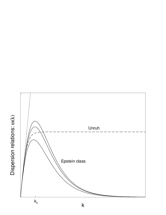
Figure 1: Shown is our family of dispersion relations, for $\beta=1$ and representatives values of $\epsilon_{1}$ (solid lines). We have also included the Unruh’s dispersion relation (dashed line) and the linear one (dotted line) for comparison.

On the other hand, the condition of a nearly linear dispersion relation for $k<k_{C}$ requires that

$$\frac{\epsilon_{1}}{2}+\frac{\epsilon_{3}}{4}=1\,.$$ (20)

Still we will have a whole family of functions parametrised by the constant $\epsilon_{1}$, as can be seen in Fig. 1.

With the change of variables $\eta\rightarrow u=exp(A|\eta|)$, the scalar wave equation (5) for the mode $\mu_{n}$ becomes:

$$\left[\partial^{2}_{u}+\frac{1}{u}\partial_{u}+V(u)\right]\mu_{n}=0\,,$$ (21)

with:

$$V(u)=\frac{\hat{\epsilon}_{1}}{u^{2}(1+u)}+\frac{\hat{\epsilon}_{3}}{u(u+1)^{2}}-\frac{(1-6\xi)}{u^{2}A^{2}}\frac{a^{\prime\prime}}{a}\,,$$ (22)

where:

$$\hat{\epsilon_{i}}=(k_{C}|\eta_{c}|)^{2}\left(\frac{n}{k_{C}}\right)^{2(1-1/\beta)}\epsilon_{i}\,.$$ (23)

In the case of conformal coupling to gravity, $\xi=1/6$, Eq. (21) is exactly solvable in terms of hypergeometric functions [14]. This is a well studied case in the context of particle creation in a curved background [13]. Even if we are not in the case of conformal coupling, the contribution

$$\frac{a^{\prime\prime}}{a}=\frac{\beta(\beta+1)}{\eta^{2}}\,,$$ (24)

is going to be negligible at early times ($\eta\rightarrow-\infty$); at late times, it can be absorbed in the dispersion relation Eq. (18) redefining the constants $\epsilon_{i}$.

As explained in Section 2, the correct initial condition is the vacuum state solution that minimizes the energy. In the case where $\epsilon_{2}\neq 0$, this vacuum state behaves as a plane wave in the asymptotic limit $\eta\rightarrow-\infty$, with $\Omega^{(in)}_{n}\rightarrow\sqrt{\epsilon_{2}}n$. However, when $\epsilon_{2}=0$ as in our case, the correct behavior of the mode function in the remote past is given by the solution of Eq. (5) in the limit $\eta\rightarrow-\infty$. The exact solution which matches this asymptotic behavior is then given by:

$$\mu^{(in)}(\eta)=C^{in}\left(\frac{1+u}{u}\right)^{d}~{}_{2}F_{1}[\frac{1}{2}+d+b,\frac{1}{2}+d-b,1+2d,\frac{1+u}{u}]\,,$$ (25)

where $C^{in}$ is a normalization constant, and

$$b = i\tilde{b}=i\sqrt{\hat{\epsilon}_{1}}\,,$$ (26)

$$d = i\tilde{d}=\sqrt{\frac{1}{4}+\hat{\epsilon}_{3}}\,.$$ (27)

At late times the solution becomes a squeezed state by mixing of positive and negative frequencies:

$$\mu_{n}\rightarrow_{\eta\rightarrow+\infty}\frac{\alpha_{n}}{\sqrt{2\Omega^{out}_{n}}}e^{-i\Omega^{out}_{n}\eta}+\frac{\beta_{n}}{\sqrt{2\Omega^{out}_{n}}}e^{+i\Omega^{out}_{n}\eta}\,,$$ (28)

with $|\beta_{n}|^{2}$ being the Bogoliubov coefficient equal to the particle creation number per mode $n$, and $\Omega^{out}_{n}\simeq\sqrt{\epsilon_{1}}n$. Using the linear transformation properties of hypergeometric functions [37], we find that

$$\left|\frac{\beta_{n}}{\alpha_{n}}\right| = e^{-2\pi\tilde{b}}\left|\frac{\cosh\pi(\tilde{d}+\tilde{b})}{\cosh\pi(\tilde{d}-\tilde{b})}\right|\,.$$ (30)

If $d$ is a real number ($\epsilon_{3}^{\prime}>-1/4$), then we obtain:

$$|\beta_{n}|^{2}=\frac{e^{-2\pi\tilde{b}}}{2\sinh 2\pi\tilde{b}}\,.$$ (31)

It is clear from Eqs. (30) and (31) that the spectrum of created particles is nearly thermal to high accuracy,

$$|\beta_{n}|^{2}\simeq e^{-4\pi\tilde{b}}\,.$$ (32)

Thus, we can immediately conclude that the CMBR spectrum is that of a (nearly) black body spectrum. That means the spectrum is (nearly) scale invariant, i.e., the spectral index is $n_{s}\simeq 1$. This is consistent with previous results obtained in the literature [6, 8, 9, 10], when using a smooth dispersion relation and the correct choice of the initial vacuum state, as discussed above. In Refs. [6] and [8], dispersion relations, that were originally applied to black hole physics [1, 2], were used in the context of cosmology. New models of dispersion relations were proposed by the authors of Refs. [9] and [10]. Our proposal for a 1-parameter class of models has a significantly different feature from the above, namely: the appearence of ultra-low frequency modes in the transplanckian regime. The implications of such a behavior for high momenta on the production of dark energy are discussed in the next section.

4 Dark Energy from the “Tail”

In Section 2 we defined the $tail$ as the range of those modes in the frequency dispersion class (originating from the transplanckian regime), whose frequency is less or at most equal to the present Hubble rate, $H_{0}$ (see Fig. 2). It then follows that they have not decayed and redshifted away but are still frozen $today$. Since $H$ has been a decreasing function of time, many modes, even those in the ultralow frequency range, have become dynamic and redshifted away one by one, everytime the above condition is broken, i.e. when the expansion rate $H$ dropped below their frequency. Clearly, the other modes have long decayed into radiation and the tail modes are the only modes still frozen. They contain vacuum energy of very short distance, hence of very low energy. The last mode in the tail would decay when and if $H=0$. When the tail modes become dynamic by acquiring a kinetic term (when $\omega(k)>H$), they decay away as gravitational waves (explained in Section 2). The $tail$ starts from some value $k_{H}$ which must be found by solving the equation

$$\omega^{2}(k_{H})=H^{2}_{0}\,.$$ (33)

The range of the modes defining the $tail$ is then for $k_{H}<k<\infty$. Their time-dependent behaviour when they decay depends on the evolution of $H$ and is complicated because they contribute to the expansion rate for $H$. Thus, their equations of motion are coupled to the Friedmann equation.

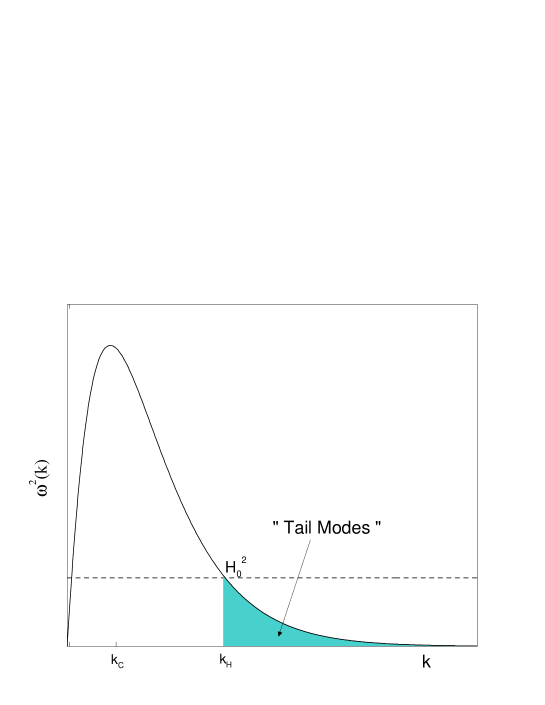
Figure 2: The range of modes in the tail, $k_{H}<k<\infty$, defined by Eq. (33). $H_{0}$ is the present value of the Hubble constant.

However we can calculate their contribution to the dark energy today, when they are still frozen, thereby mimicking a cosmological constant. We calculate numerically (using ’Mathematica’) the range of the modes in the tail from Eq. (33) and use this value for the limit of integration in the tail energy given by Eq. (15). Below we report these results for the case of a scale factor with $\beta=1$ but other values of $\beta$ were also considered numerically and they produce an even smaller dark energy due to the extra suppression in the integral coming from the Bogoliubov coefficient $\beta_{k}^{2}$. Eq. (33) is a messy transcendental equation but the solution to that equation is crucial to the dark energy since the value $k_{H}$ is the limit of the energy integral. That is why we solved Eq. (33) numerically and replaced it in Eq. (15) for the energy, using different representative values of the parameter $\epsilon_{1}$.

The energy for the tail is given by:

$$\langle\rho_{tail}\rangle=\frac{1}{2\pi^{2}}\int^{\infty}_{k_{H}}kdk\int\omega(k)d\omega~{}|\beta_{k}|^{2}\,,$$ (34)

while the expression for the total energy is:

$$\langle\rho_{total}\rangle=\frac{1}{2\pi^{2}}\int^{\infty}_{0}kdk\int\omega(k)d\omega~{}|\beta_{k}|^{2}\,.$$ (35)

The numerical calculation of the tail energy produced the following result: for random different values of the free parameters, the dark energy of the tail is $\rho_{tail}=10^{-122}f(\epsilon_{1})$, times less than the total energy during inflation, i.e. $\frac{\rho_{tail}}{\rho_{total}}=10^{-122}f(\epsilon_{1})$ at Planck time. The prefactor $f(\epsilon_{1})$, which depends weakly on the parameter of the dispersion family $\epsilon_{1}$, is a small number between 1 to 9, which clearly can contribute at the most by 1 order of magnitude.

This is an amazing result! It can readily be checked by plugging in the dispersion expression for $\omega_{k}$, Eq. (17), in the integral expression of Eq. (34) for the tail energy, then using as the limit of integration the value $k_{H}$ found by the condition in Eq. (33). This result can be understood qualitatively by noticing that the behavior of the frequency for the “tail” modes is nearly an exponential decay (see Eq. (17)), and as such dominates over the other terms in the energy integrand of Eq. (34):

$$\omega^{2}(k>k_{C})\approx exp(-k/k_{C})\,,$$ (36)

Hence, due to the decaying exponential, the main contribution to the energy integral in Eq. (34) comes from the highest value of this exponentially decaying frequency, which is the value of the integrand at the tail starting point, $k_{H}\sim O(M_{P})$, i.e.,

$$\langle\frac{\rho_{tail}}{\rho_{total}}\rangle\approx\frac{k_{H}^{2}}{M_{P}^{4}}\omega^{2}(k_{H})\approx\frac{H_{0}^{2}}{M_{P}^{2}}\approx 10^{-122}\,.$$ (37)

Due to the physical requirement that the tail modes must have always been frozen, the tail starting frequency $\omega(k_{H})$ is then proportional to the current value of Hubble rate $H_{0}$ (Eq. (33)).

We suspect this result is generic for any scenario that features ultralow frequencies which exponentially decay to zero at very high momenta for two reasons. First, all the modes with an ultralow frequency $\omega<H_{0}$ will be frozen and thus produce dark energy. Secondly, their contribution to the energy may be small because of the following. Due to this kind of dispersion in the high momentum regime, the phase space available for the ultra-low frequency modes with $\omega(k>k_{C})$ gets drastically reduced when compared to the phase space factor in the case of a non-dispersive transplanckian regime, controlling in this way these modes contribution to the energy density. The result for the tail energy also means that the tail energy dominates today’s expansion of the universe. Thus, at present, we can not tell a priori the evolution of these modes and the time when they may become dynamic. Only the solution to the equation for the modes coupled (strongly at present) to the Friedmann equation would answer the question as to whether $H$ will continue to decrease whith time. If that were the case, then these tail modes would also eventually become dynamic and decay. However, we calculated the equation of state for the limiting case when $H=0$. In this case, all the modes in the tail are dynamic. The calculation of the energy density of the tail in the dynamic case from Eq. (15) confirms that the tail decays in the form of radiation, as expected since their physical nature is that of gravity waves of very short distances (but ultralow energy), originating from tensor perturbations during inflation.

The opposite case is also a possible outcome to the coupled equations. It’s possible that the frozen modes of the tail will prevent $H$ from dropping further below, in which case these modes will never decay. We have not solved these coupled equation yet, therefore we are just speculating on the two possible outcomes of that calculation. The solution is left for future work.

At present, these modes, originating from the transplanckian regime, are behaving as dark energy of the same magnitude as the current total energy in the universe. This idea is then a leap forward to this longstanding and challenging problem of dark energy, for at least two reasons: first, inspired by superstring duality, it is very plausible to speak of scenarios with ultralow frequencies and very high momenta. The tail modes, that are frozen at present, provide a good candidate for the dark energy as our calculations show. Secondly, although smooth dispersion functions that model the transplanckian regime do not affect the CMBR spectrum, this regime still leaves its imprints in the contribution to the energy of the universe. This is a rich and currently underexplored area to consider with respect to the cosmological constant mystery.

5 Conclusions

In this work we investigated two phenomenological aspects of transplanckian physics: the issue of dark energy production, and the sensitivity of the observed CMBR spectrum to the transplanckian regime. For this purpose, a family of dispersion relations is introduced that modulate the high frequencies of the inflationary perturbation modes at large values of the momenta $k$ for the transplanckian regime. The smooth dispersion relations are chosen such that the frequency graph attenuates to zero at very high $k$, thereby producing ultralow frequencies corresponding to very short distances, but it is nearly linear for low values of $k$ up to the cuttoff scale $k_{C}=M_{P}$.

We present the exact solutions to the mode equations and calculate the spectrum through the method of Bogoliubov coefficients. The resulting CMBR spectrum is shown to be (nearly) that of a black body. This calculation lends strong support to the conjecture that smooth dispersion relations which ensure an adiabatic time-evolution of the modes produce a nearly scale invariant spectrum. Further, we elaborate on the issue of the initial conditions to which the spectrum is highly sensitive and show that there is no ambiguity in the correct choice of the initial vacuum state. The only initial vacuum is the adiabatic vacuum obtained by the solution to the mode equation. On the other hand, we showed that the assumption of neglecting the possible back reaction effects of the tail modes on the inflaton field is reasonable and is justified by the result of the tail energy calculation of Section 4. Also the Bogoliubov coefficient obtained, Eq. (29), is exponentially suppressed, so back-reaction does not become significant. We would also like to stress that due to the dispersion class of functions chosen, defined in the whole range of momenta from zero to infinity, the total energy contribution of the modes produced is finite, without the need of applying any renormalization/subtraction scheme. In a sense, the regularization-renormalization procedure is encoded in the class of dispersion we postulate.

The most exciting result of this work is the generation of dark energy in the observed amount for the present universe [12]. This has its origin at the transplanckian regime, due to the presence of the dispersed tail modes with ultralow frequencies equal or less than the current Hubble constant. The evolution of these modes is given by their equation of motion, and it depends on the Hubble rate through the friction-like term $3H_{0}\dot{\mu}_{n}$. On the other hand, the evolution of the Hubble rate, given by the Friedmann equation, contains contribution from the energy of these modes. But currently, the Hubble constant dominates over their frequency in the mode equation of motion. It then follows that the tail modes, up to present, are still frozen and have been behaving like a cosmological constant term. Therefore their energy is dark energy.

We have calculated numerically the energy of the $tail$ during the inflationary stage for different values of the dispersion parameter $\epsilon$. The calculation showed that the tail energy was $10^{-122}$ (times a prefactor $f(\epsilon_{1})$ which weakly depends on $\epsilon_{1}$ and, for random values of the parameter, takes values between 1 to 9) orders less than the total energy during inflation. This result is true for the whole class of dispersion relations. We chose different random values of the 1-parameter dispersion family $\epsilon_{1}$, and the numerical calculation shows that $\epsilon_{1}$ influences the energy at the most by less than an order of magnitude. We did not need to do any tuning of the parameters and used the Planck scale as the fundamental scale of the theory. Clearly, at present the tail energy dominates in the Friedmann equation, if the ratio of its energy to the total energy (as found by the calculation) was $10^{-122}f(\epsilon_{1})$ during inflation. The $tail$ thus provides a strong candidate for explaining the dark energy of the universe [12]. We suspect that the above result of producing such an extremely small number for the $tail$ energy without any fine-tuning (and by using $M_{P}$ as the only fundamental scale of the theory), is generic for any dispersion graph with a $tail$. The family of dispersion relations that feature a $tail$, corresponding to vacuum modes of very short distances, was motivated by superstring duality [28, 29].

However, in Section 2 we made the observation that introducing a dispersion relation is equivalent to introducing changes in the curvature of the universe, at very short or very large distances while keeping the generalized frequency $\Omega_{n}$ of Eq. (5) invariant. It is quite possible that the dispersion relation for the $tail$ modes results from a different curvature of the universe at very short distances. This is an important link and we use it in a sequential paper [36] to demonstrate that the SN1a data can not be reinterpreted away by changing the large scale curvature of the universe. Although it is counterintuitive, since large distance would correspond to low energy theories, we show in [36] that any changes in large scale curvature would disagree with the observed CMBR spectrum.

It would be interesting to know what happens to the tail and the Hubble rate in the future. After all, a model is useful in so far as it can make future predictions. Although conceptually it is straightforward to find out the answer, given by the solution to the coupled equations (5), (7) and (8), technically it appears difficult to predict the future evolution of the tail modes. The technical difficulty lies in the fact that at present, the $tail$ equation of motion is strongly coupled to the Friedmann equation for $H$ since the $tail$ energy dominates. The Hubble rate would continue to decrease only if these modes decay, but these modes can decay only when the Hubble rate decreases below their frequency. It may be possible that the frozen tail will sustain a constant Hubble rate which in turn will not allow the further decay of the tail modes. It is also possible that $H$ will continue to decrease in which case the tail modes will become dynamic and redshift away in the future. It is only the solution to the mode equations coupled to the Friedmann equation, that will provide the answer on whether the Hubble constant and tail will decay in the future or remain at their current value. We do not have this solution yet, and the work is left for future investigation. In addition, the equation of state, $w(t)=\langle p/\rho\rangle$, is an $observable$ that will provide a test to the model [40], especially with the new data coming in the near future from the SNAP [41] and SDSS [42] missions.

However, we know that currently these $tail$ modes are frozen vacuum modes of ultralow energy but very short distance, thus their energy behaves like a cosmological constant energy. We also know they become dynamic and acquire a kinetic term only when the Hubble rate drops below the frequency. And, if they decay, the product is radiation of gravity waves at very short distances since their physical origin is from the tensor perturbations during inflation (it is well known that scalar perturbations do not contribute to the energy). The condition for the decay of the last mode in the tail is fulfilled when $H$ has dropped to zero.

Many of our results, e.g. the dispersion family and the exact solutions together with the Bogoliubov coefficients, could be applied to the Black Hole Physics. The issue of transplanckian physics was originally raised in the Black Hole context with respect to the sensitivity of the Hawking radiation to the blueshifted, superplanckian energy wavepackets. Following a phenomenological approach, a few dispersive models were introduced [1]-[5] in order to introduce a bound on the blueshifted energies and check the sensitivity of the black hole spectrum. We have introduced a new, different family of dispersive models, that also gives rise to a thermal spectrum. The analytical results of our class of dispersion models can be applied to the black hole physics and reproduce the same thermal Hawking spectrum. There are many subtleties involved due to the different symmetries of the two scenarios, but these issues are beyond the purpose and scope of this paper. It is left for future work. However, if the Hawking radiation for this class of dispersions is again thermal, it lends strong support to Unruh’s conjecture that black hole radiation is insensitive to physics in the far ultraviolet (trans-planckian) regime, being predominantly an infrared effect. On the other hand, our class of models departs from the previous ones in the asymptotic behavior at very high momenta, with the presence of an infinite “tail” of ultralow frequency modes. The $tail$ feature and energy results, applied to a black hole case, may raise interesting issues, in particular with respect to the black hole’s information loss paradox.

Acknowledgment: We are very grateful to A. Riotto for many beneficial comments and for pointing out the connection with superstring duality. We also want to thank R. Barbieri, R. Rattazzi, L. Pilo, S. Carroll, C. T. Hill for helpful discussions. P.K. would like to acknowledge financial support by EC under the TMR contract No. HPRN-CT-2000-00148.

References

- [1] T. Jacobson, Phys. Rev. D44, 1731 (1991); D48, 728 (1993); for a review, see hep-th/0001085.
- [2] W. Unruh, Phys. Rev. D51, 2827 (1995).
- [3] R. Brout, S. Massar, R. Parentani and P. Spindel, Phys. Rev. D52, 4559 (1995).
- [4] N. Hambli and D. Burgess, Phys. Rev. D53, 5717 (1996).
- [5] S. Corley and T. Jacobson, Phys. Rev. D54, 1568 (1996); S. Corley, Phys. Rev. D57, 6280 (1998).
- [6] J. Martin and R. H. Brandenberger, hep-th/0005209; R. H. Brandenberger and J. Martin, astro-ph/0005432.
- [7] B. L. Hu, gr-qc/9511077.
- [8] J. C. Niemeyer, Phys. Rev. D63, 123502 (2001); J. C. Niemeyer and R. Parentani, astro-ph/0101451.
- [9] J. Kowalski-Glikman, Phys. Lett. B499,1 (2001) .
- [10] A. Kempf, Phys. Rev. D63, 083514 (2001); A. Kempf and J. C. Niemeyer, astro-ph/0103225.
- [11] R. Easther, B. R. Green, W. H. Kinney and G. Shin, hep-th/0104102.
- [12] S. Perlmutter, M. S. Turner and M. White, Phys. Rev. Lett. 83, 630 (1999).
- [13] L. Parker, Phys. Rev. 183, 1057 (1969); R. U. Sexl and H. K. Urbantke, Phys. Rev. 179, 1247 (1969); Y. Zel’dovich and A. Starobinsky, Zh. Sksp. Teor. Fiz. 61, 2161 (1971) [Sov. Phys. JETP 34, 1159 (1971)]; Ya. Zel’dovich, Pis’ma Zh. Eksp. Teor. Fiz. 12, 443 (1970) [Sov. Phys. JETP Lett. 12, 302 (1970)]; B. L. Hu, Phys. Rev. D9, 3263 (1974); S. W. Hawking, Nature 248, 30 (1974); Comm. Math. Phys. 43, 199 (1975); W. G. Unruh, Phys. Rev. D14, 870 (1976); B. K. Berger, Phys. Rev. D12, 368 (1975); L. Mersini, Int. J. Mod. Phys. A13, 2123 (1998).
- [14] P. S. Epstein, Proc. Nat. Acad. Sci., 16, 627 (1930); L. Parker, Nature 261, 20 (1976); in “Asymptotic Structure of Space-Time”, eds. F. P. Esposito and L. Witten (Plenum, New York, 1977).
- [15] T. Tanaka, astro-ph/0012431.
- [16] A. A. Starobinsky, astro-ph/0104043.
- [17] E. M. Lifshitz and I. M. Khalatnikov, Adv. Phys. 12, 185 (1963).
- [18] L. P. Grishchuk, Phys. Rev. D50, 7154 (1994).
- [19] L. P. Grishchuk, Zh. Eksp. Teor. Fiz. 67, 825 (1974).
- [20] J. Martin and D. Schwarz, Phys. Rev. D57, 3302 (1998).
- [21] For a review, see for example: V. Mukhanov, H. Feldman and R. H. Brandenberger, Phys. Rep. 215, 203 (1992), and references therein.
- [22] S. Corley and T. Jacobson, Phys. Rev. D54, 1568 (1996); Phys. Rev. D59, 124011 (1999).
- [23] W. G. Unruh, Phys. Rev. Lett. 46, 1351 (1981); D. A. Lowe et al., Phys. Rev. D52, 6997 (1995); M. Visser, Class. Quant. Grav. 15, 1767 (1998); T. A. Jacobson and D. Mattingly, gr-qc/0007031; hep-ph/0009051.
- [24] B. L. Hu and Y. Zhang, “Coarse-graining, scaling and inflation”, Univ. Maryland preprint 90-186 (1990); B. L. Hu, in “Relativity and Gravitation: Classical and Quantum”, Proc. SILARG VII, Cocoyoc, Mexico, 1990, eds. J. C. D’ Olivo et al. (World Scientific, Singapore 1991).
- [25] A. Albrecht and P. Steinhardt, Phys. Rev. Lett. 48, 1220 (1982); L. A. Kofman et al., Phys. Rev. B157, 361 (1985); A. Albrecht, in Proc. “The Santa Fe TASI 87”, eds. R. Slansky and G. West, World Scientific (1998); N. B. Kopnin and G. E. Volovik, Phys. Rev. B57, 8525 (1998); T. A. Jacobson and G. E. Volovik, Phys. Rev. D58, 064021 (1998); G. L. Kane, Phys. Rep. 307, 197 (1998); A. A. Starobinsky, JETP Lett. 68, 757 (1998); Nature 331, 673 (1998); M. S. Turner, astro-ph/9912211; P. J. Steinhardt et al., astro-ph/0006373; D. Huterer and M. S. Turner, astro-ph/0012510.
- [26] E. W. Kolb and M. S. Turner, “The Early Universe” (Addison-Wesley, Menlo Park, Ca. 1990).
- [27] A. Linde, “Particle physics and inflationary cosmology” (Harwood Academic Publishers, Switzerland, 1990)
- [28] M. B. Green, J. H. Schwarz and E. Witten, “Superstring Theory. Vol. 1&2” (Cambridge University Press, Cambridge, 1987).
- [29] R. Brandenberger and C. Vafa, Nucl. Phys. B316, 391 (1989).
- [30] L. Kofman, A. Linde and A. A. Starobinsky, Phys. Rev. Lett. 76, 1011 (1996).
- [31] L. A. Kofman, A. D. Linde and A. A. Starobinsky, Phys. Rev. Lett. 73, 3195 (1994); L. Kofman, A. Linde and A. Starobinsky, Phys. Rev. D56, 3258 (1997).
- [32] J. H. Traschen, R. H. Brandenberger, Phys. Rev. D 42, 2491 (1990); Y. Shtanov, J. Traschen and R. Brandenberger, Phys. Rev. D51, 5438 (1995).
- [33] T. D. Bunch and P. C. W. Davies, Proc. Roy. Soc. Lond. A360, 117 (1978).
- [34] N. D. Birrell and P. C. W. Davies, “Quantum fields in curved space-time” (Cambridge University Press, Cambrigde, 1982).
- [35] G. Felder, L. Kofman and A. Linde, JHEP 0002:027 (2000).
- [36] M. Bastero-Gil and L. Mersini, “Large Scale Curvature and SN1a data”, in preparation.
- [37] M. Abramowitz and A. I. Stegun (eds.), “Handbook of Mathematical Functions” (New York, Dover, 1965).
- [38] N. Tsamis and R. Woodard, Phys. Lett. B301, 351 (1993); Nucl. Phys. B474, 235 (1996); Ann. Phys. 267, 145 (1998).
- [39] R. H. Brandenberger, hep-th/0004016.
- [40] D. Huterer and M. Turner, astro-ph/0012510.
- [41] http://snap.lbl.gov
- [42] http://www.sdss.org