Heavy quark production at high energy

Abstract:

We report on QCD radiative corrections to heavy quark production valid at high energy. The formulae presented will allow a matched calculation of the total cross section which is correct at $O(\alpha_{s}^{3})$ and includes resummation of all terms of order $\alpha_{s}^{3}[\alpha_{s}\ln(s/m^{2})]^{n}$. We also include asymptotic estimates of the effect of the high energy resummation. A complete description of the calculation of the heavy quark impact factor is included in an appendix.

1 Introduction

In this paper we report on the calculation of the strong radiative corrections to the  process

$$p+\bar{p}\longrightarrow b+\bar{b}+X\,.$$ (1)

This reconsideration is prompted in part by the fact that measurements at the Fermilab Tevatron [1]–[4] indicate that the $b$ cross section lies above the predictions [5, 6] from $O(\alpha_{s}^{3})$ perturbation theory [5, 7]. Similar excesses have been reported recently in the photoproduction $b$ cross-section [8, 9], and in $b$ production in $\gamma\gamma$ collisions [10, 11]. Two remarks need to be made about this situation. First, the transformation of the observed experimental cross section to a $b$-quark cross section requires the inclusion of fragmentation and decay corrections which are subject to theoretical errors. Although these corrections may be smaller when we consider the $b$-jet cross section [12] rather than the $b$-quark cross section, experimental results for the $b$-jet cross section still indicate an excess over theoretical predictions [13]. Second, the fixed order perturbation theory description of $b$-quark production receives large corrections in order $\alpha_{s}^{3}$ which call into question the validity of perturbation theory. We may simply conclude that, in this energy and mass range, the $\alpha_{s}^{3}$ theory is not very predictive and ignore the disagreement with experiment as an inadequacy of the theory. A more constructive approach, which we adopt in this paper, is to try and resum the large corrections.

The heavy quark cross section is calculable because the heavy quark mass $M$ is larger than the QCD scale $\Lambda$. As first observed in ref. [5] the large corrections in $O(\alpha_{s}^{3})$ come both from the threshold region $s\sim M^{2}$ and from the the high energy region $s\gg M^{2}$, where $s$ is the normal Mandelstam variable for the parton sub-process.

The resummation of the threshold soft gluon corrections is best carried out in $\omega$-space, where $\omega$ is the moment variable after Mellin transform with respect to $s$. In $\omega$-space the threshold region corresponds to the limit $\omega\rightarrow\infty$ and the structure of the threshold corrections is as follows

$$\hat{\sigma}=\sigma^{LO}\left\{1+\sum_{j=1}^{\infty}\sum_{k=1}^{2j}b_{jk}\alpha_{s}^{j}\ln^{k}\omega\right\}.$$ (2)

Detailed studies [14] indicate that such threshold resummation is of limited importance at the Tevatron where $b$-quarks are normally produced far from threshold. Resummation effects lead to minor changes in the predicted cross section and only a slight reduction in the scale dependence of the results.

At high energy, heavy quark production becomes a two scale problem, since $S\gg M^{2}\gg\Lambda^{2}$ and the short distance cross section contains logarithms of $s/M^{2}$. As we proceed to higher energies such terms can only become more important, so an investment in understanding these terms at the Tevatron will certainly bear fruit at the LHC. At small $\omega$ the dominant terms in the heavy quark production short distance cross section are of the form

$$\hat{\sigma}\sim\frac{\alpha_{s}^{2}}{M^{2}}\sum_{j=0}^{\infty}\alpha_{s}^{j}\sum_{k=0}^{\infty}c_{jk}\left(\frac{\alpha_{s}}{\omega}\right)^{k}.$$ (3)

For $j=0$ we obtain the leading logarithm series (LLx). Resummation of these terms has received considerable theoretical attention in the context of the $k_{T}$-factorization formalism [15]–[21]. Although some work quantitative nature has been performed [22, 23], so far the connection with the precise structure function data has been indirect since the unintegrated gluon distributions are not measured directly. In addition, both the difficulty in reconciling $k_{T}$-factorization with structure function data from HERA [24]–[29], and the theoretical uncertainty in the face of large [30] destabilizing subleading corrections [31]–[34] have hampered this program. However significant progress in understanding the origin and resolution of these instabilities has been made recently [35]–[38], and resummed parton densities in the small $x$ region can be determined from HERA data [39]. Consistent resummed calculations of heavy quark production cross-sections are thus finally a possibility.

The aim of this paper is to collect together the relevant results for a quantitative calculation of the total heavy quark production cross section. Our formulae include the known fixed order results, as well as the resummation of the leading tower of high energy logarithms. The approach to this resummation is as follows. The $O(\alpha_{s}^{2})$ and $O(\alpha_{s}^{3})$ total cross sections are well known at the parton level. Using the results of the $k_{T}$-factorization, valid at high energy, we can resum the logarithms of $s/M^{2}$ by determining the leading coefficients $c_{0k}$ of eq. (3) for $k=2,\dots,\infty$, resumming the singularities using the techniques of ref. [38], and then combining with resummed parton distributions [39] to give a high-energy improved short distance cross section.

This paper deals exclusively with results for the total cross section. This quantity is not experimentally accessible with current detectors which typically have a $p_{T}$ threshold below which $b$-quarks cannot be observed. The technical problems of extending this analysis to less inclusive measurements may be formidable. The present analysis is intended to give us an understanding of the size of these terms, before undertaking the extension to experimentally more realistic quantities.

The structure of this paper is as follows. In section 2, we consider the description of the direct component of bottom quark photoproduction both in fixed order perturbation theory and in the framework of $k_{T}$-factorization. We use the latter formalism as a technical device to resum the logarithms of $s/M^{2}$ and cast the final result in the form of a high-energy improved collinear factorization formula. Section 3 repeats similar steps for the hadroproduction of heavy flavours. In practice, the treatment of the photoproduction of heavy flavours is more complex than described in section 2 because of the hadronic (resolved) component of the photon. The resolved component of the photoproduction cross section should be treated by the methods of section 3. Similar remarks apply to heavy quark production in $\gamma\gamma$ collisions. Section 4 presents some analytic estimates. In section 5 we draw some preliminary conclusions. A complete description of the calculation of the heavy flavour impact factors is presented in appendix A.

2 Photoproduction of heavy flavours

2.1 Fixed order perturbation theory

In this section we report on the results for the direct component of the photoproduction of heavy flavours in fixed order perturbation theory [40]. We first define reduced cross sections $\Sigma$ with the mass dimensions removed, both at the hadronic and partonic level,

$$\Sigma(\rho)=M^{2}\sigma(M^{2},S)\,,\qquad\hat{\Sigma}_{\gamma j}\left(\hat{\rho},\frac{\mu^{2}}{M^{2}}\right)=M^{2}\hat{\sigma}_{\gamma j}(s,M^{2},\mu^{2})\,.$$ (4)

Here $S$ and $s$ are the squares of the total hadronic and partonic centre of mass energies, respectively, $M$ the mass of the heavy quark, $\rho=4M^{2}/S,\hat{\rho}=4M^{2}/s=\rho/x$ and $\mu$ is the renormalization and factorization scale. We can further express the partonic cross section as

$$\hat{\Sigma}_{\gamma j}\left(\hat{\rho},\frac{\mu^{2}}{M^{2}}\right)=\alpha_{em}\alpha_{s}(\mu^{2})f_{\gamma j}\left(\hat{\rho},\frac{\mu^{2}}{M^{2}}\right).$$ (5)

The photon-hadron cross section is then given by the collinear factorization formula

$$\Sigma(\rho)=\alpha_{em}\alpha_{s}(\mu^{2})\int_{\rho}^{1}\frac{dx}{x}\sum_{j=q,\bar{q},g}f_{\gamma j}\left(\frac{\rho}{x},\frac{\mu^{2}}{M^{2}}\right)F^{j}(x,\mu^{2})\,,$$ (6)

where $F^{j}(x,\mu^{2})=xq(x,\mu^{2}),x\bar{q}(x,\mu^{2}),xg(x,\mu^{2})$, $j=q,\bar{q},g$ are the parton momentum densities, renormalized in $\overline{\mathrm{MS}}$ at scale $\mu$. The coefficient functions $f_{\gamma j}$ have a perturbative expansion which, following ref. [40], we write as,

$$f_{\gamma j}\left(\rho,\frac{\mu^{2}}{M^{2}}\right)=f^{(0)}_{\gamma j}(\rho)+4\pi\alpha_{s}(\mu^{2})\left[f^{(1)}_{\gamma j}(\rho)+\bar{f}^{(1)}_{\gamma j}(\rho)\ln\frac{\mu^{2}}{M^{2}}\right]+O(\alpha_{s}^{2})\,.$$ (7)

The functions $f_{\gamma j}$ depend on the charge of the quark which interacts with the photon. To make these dependences explicit we further define the quantities,

$$f_{\gamma g}\left(\rho,\frac{\mu^{2}}{M^{2}}\right) = e_{Q}^{2}c_{\gamma g}\left(\rho,\frac{\mu^{2}}{M^{2}}\right),$$

$$f_{\gamma q}\left(\rho,\frac{\mu^{2}}{M^{2}}\right) = f_{\gamma\bar{q}}\left(\rho,\frac{\mu^{2}}{M^{2}}\right)=e_{Q}^{2}c_{\gamma q}\left(\rho,\frac{\mu^{2}}{M^{2}}\right)+e_{q}^{2}d_{\gamma q}\left(\rho,\frac{\mu^{2}}{M^{2}}\right),$$ (8)

where $e_{q}$ is the charge of the incoming light quark, while $e_{Q}$ is the charge of the heavy quark. Results for the perturbative expansions of the functions, $c_{\gamma g},c_{\gamma q}$ and $d_{\gamma g}$ are given in ref. [40].

We can also define the moments $f_{\omega}$ of all functions $f$,

$$f_{\omega}=\int_{0}^{1}d\rho\;\rho^{\omega-1}f(\rho)\,,\qquad F_{\omega}(\mu^{2})=\int_{0}^{1}dx\;x^{\omega-1}F(x,\mu^{2})\,.$$ (9)

Taking moments of eq. (6) we get

$$\Sigma_{\omega}=\int_{0}^{1}d\rho\;\rho^{\omega-1}\Sigma(\rho)=\alpha_{em}\alpha_{s}(\mu^{2})\sum_{j=q,\bar{q},g}f_{\gamma j\;\omega}\left(\frac{\mu^{2}}{M^{2}}\right)F^{j}_{\omega}(\mu^{2})\,.$$ (10)

The moments of $c_{\gamma g},c_{\gamma q}$ and $d_{\gamma g}$ are easily obtained from the results of [40]. The expressions for the partonic cross-sections $\hat{\Sigma}$ are then

$$\hat{\Sigma}^{\gamma g}_{\omega}\left(\frac{\mu^{2}}{M^{2}}\right) = e_{Q}^{2}\alpha_{em}\alpha_{s}\left(c_{\gamma g\;\omega}^{(0)}+4\pi\alpha_{s}\left[c_{\gamma g\;\omega}^{(1)}+\ln\left(\frac{\mu^{2}}{M^{2}}\right)\bar{c}_{\gamma g\;\omega}^{(1)}\right]\right),$$

$$\hat{\Sigma}^{\gamma q}_{\omega}\left(\frac{\mu^{2}}{M^{2}}\right) = \alpha_{em}\alpha_{s}^{2}4\pi\left(e_{q}^{2}\left[d_{\gamma q\;\omega}^{(1)}+\ln\left(\frac{\mu^{2}}{M^{2}}\right)\bar{d}_{\gamma q\;\omega}^{(1)}\right]\right.+$$ (11)

$$\hphantom{\alpha_{em}\alpha_{s}^{2}4\pi\Bigg{(}}\!\left.+\,e_{Q}^{2}\left[c_{\gamma q\;\omega}^{(1)}+\ln\left(\frac{\mu^{2}}{M^{2}}\right)\bar{c}_{\gamma q\;\omega}^{(1)}\right]\right).$$

The form of these results in the high energy limit are then readily derived [15]: as $\omega\rightarrow 0$

$$\hat{\Sigma}^{\gamma g}_{\omega}\left(\frac{\mu^{2}}{M^{2}}\right) \sim \pi e_{Q}^{2}\alpha_{s}\alpha_{em}\left[\frac{7}{9}+\left(\frac{41}{27}-\frac{7}{9}\ln\frac{\mu^{2}}{M^{2}}\right)\frac{a}{\omega}\right]+\cdots\,,$$

$$\hat{\Sigma}^{\gamma q}_{\omega}\left(\frac{\mu^{2}}{M^{2}}\right) \sim \pi e_{Q}^{2}\alpha_{s}\alpha_{em}\frac{V_{c}}{2N_{c}^{2}}\left(\frac{41}{27}-\frac{7}{9}\ln\frac{\mu^{2}}{M^{2}}\right)\frac{a}{\omega}+\cdots\,,$$ (12)

where as usual $a=N_{c}\alpha_{S}/\pi$, and $V_{c}=N_{c}^{2}-1$. The $d_{\gamma g}$ terms are non singlet, and thus contain no $\omega=0$ singularities.

2.2 High energy behaviour

We now turn to the high energy behaviour of the photoproduction cross sections which contain logarithms of $s/M^{2}$ and need to be resummed. This resummation is performed by using the ${\mathbf{k}}$-factorized expression for the cross section

$$\Sigma(\rho)=\sum_{j=q,\bar{q},g}\int\;\frac{dx}{x}\;\frac{d^{2}{\mathbf{k}}}{\pi}\;\hat{\Sigma}_{\gamma j}\left(\frac{\rho}{x},{\mathbf{k}},M^{2},\mu^{2}\right)\mathcal{F}^{j}(x,{\mathbf{k}}^{2},\mu^{2})\,,$$ (13)

The functions $\mathcal{F}^{j}$ are the unintegrated parton distribution functions and $\hat{\Sigma}_{\gamma j}$ are the (lowest-order and gauge-invariant) off-shell continuations of the parton cross sections. The diagrams necessary to calculate $\hat{\Sigma}$ are illustrated in figure 1 where $k_{2}=xp_{2}+{\mathbf{k}}$. We can simplify eq. (13) by taking the moments with respect to the longitudinal variable, cf. eq. (9), to undo the convolution:

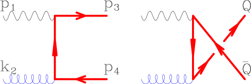
Figure 1: Diagrams for the direct component of heavy quark photoproduction at high energy.

$$\Sigma_{\omega}=\sum_{j=q,\bar{q},g}\int\frac{d^{2}{{\mathbf{k}}}}{\pi}\;J^{j}_{\omega}\left(\frac{{\mathbf{k}}^{2}}{M^{2}},\frac{{\mu}^{2}}{M^{2}}\right)\mathcal{F}^{j}_{\omega}({\mathbf{k}}^{2};\mu)\,.$$ (14)

$J^{j}_{\omega}$ is the impact factor which expresses the response of the quark-antiquark pair as a function of the transverse momentum of the incoming light parton. A further simplification can be achieved by defining Mellin transforms with respect to the transverse momentum squared variables:

$$\mathcal{F}_{\omega}(\gamma) = \int_{-\infty}^{\infty}\frac{d^{2}{\mathbf{k}}}{\pi}\left(\frac{{\mathbf{k}}^{2}}{\mu^{2}}\right)^{-\gamma}\mathcal{F}_{\omega}({\mathbf{k}}^{2},\mu^{2})\,,$$

$$J_{\omega}(\gamma) = \int_{-\infty}^{\infty}\frac{d^{2}{\mathbf{k}}}{{\pi\mathbf{k}}^{2}}\left(\frac{{\mathbf{k}}^{2}}{M^{2}}\right)^{\gamma}J_{\omega}\left(\frac{{\mathbf{k}}^{2}}{M^{2}},\frac{{\mu}^{2}}{M^{2}}\right),$$ (15)

where the dependence of the Mellin transforms on $\mu^{2}$ has now been suppressed. The Mellin transform of $\mathcal{F}$ is defined on the fundamental strip $\alpha<\mathop{\rm Re}\nolimits(\gamma)<\beta$ corresponding to the assumed behaviours

$$\mathcal{F}_{\omega}({\mathbf{k}}^{2},\mu^{2}) \sim ({\mathbf{k}}^{2})^{\alpha-1}\,,\qquad{\mathbf{k}}^{2}\rightarrow\infty\,,$$

$$\mathcal{F}_{\omega}({\mathbf{k}}^{2},\mu^{2}) \sim ({\mathbf{k}}^{2})^{\beta-1}\,,\qquad{\mathbf{k}}^{2}\rightarrow 0\,.$$

The existence of the integrated parton distributions

$$F_{\omega}(\mu^{2})=\int_{0}^{\mu^{2}}d{\mathbf{k}}^{2}\mathcal{F}_{\omega}({\mathbf{k}}^{2},\mu^{2})$$ (16)

implies that $\beta>0$. For the impact factor $J$ the Mellin transform is defined in the strip $0<\mbox{Re}(\gamma)<1$. The inverse Mellin transforms are defined as,

$$\mathcal{F}_{\omega}({\mathbf{k}}^{2},\mu^{2}) = \frac{1}{{\mathbf{k}}^{2}}\int_{C}\frac{d\gamma}{2\pi i}\left(\frac{\mathbf{k}^{2}}{\mu^{2}}\right)^{\gamma}\mathcal{F}_{\omega}(\gamma)\,,$$

$$J_{\omega}\left(\frac{{\mathbf{k}}^{2}}{M^{2}},\frac{{\mu}^{2}}{M^{2}}\right) = \int_{C}\frac{d\gamma}{2\pi i}\left(\frac{M^{2}}{\mathbf{k}^{2}}\right)^{\gamma}J_{\omega}(\gamma)\,,$$ (17)

where $C$ is a contour lying in the fundamental strips defined above. Inserting these expressions in the representation, eq. (14), and performing the transverse momentum integration we then have

$$\Sigma_{\omega}=\sum_{k=q,\bar{q},g}\int_{C}\;\frac{d\gamma}{2\pi i}\left(\frac{M^{2}}{\mu^{2}}\right)^{\gamma}J^{k}_{\omega}(\gamma)\;\mathcal{F}^{k}_{\omega}(\gamma)\,.$$ (18)

To understand how this result may be used to resum high energy logarithms, consider first the unintegrated gluon density $\mathcal{F}^{g}_{\omega}({\mathbf{k}}^{2},\mu^{2})$ as a solution to the BFKL equation: the Mellin transform $\mathcal{F}^{g}_{\omega}(\gamma)$ then has the form

$$\mathcal{F}^{g}_{\omega}(\gamma)=\frac{\mathcal{F}^{(0)}_{\omega}(\gamma)}{1-\frac{a}{\omega}\chi_{0}(\gamma)}\,,$$ (19)

where $\chi_{0}(\gamma)=2\psi(1)-\psi(\gamma)-\psi(1-\gamma)$ is the Mellin transform of the lowest order BFKL kernel. Assuming that the asymptotic behaviour $(\mathbf{k}^{2}\gg\mu^{2})$ is determined perturbatively (rather than by the properties of $\mathcal{F}^{(0)}_{\omega}$), the rightmost singularity of $\mathcal{F}^{g}_{\omega}(\gamma)$ is then a simple pole in the fundamental strip at $\gamma=\gamma_{s}(a/\omega)$, where $\gamma_{s}(a/\omega)$ is defined implicitly through the relation

$$\frac{a}{\omega}\chi_{0}\left(\gamma_{s}\left(\frac{a}{\omega}\right)\right)=1\,,$$ (20)

and the condition $\gamma_{s}(0)=0$. When expanded perturbatively we have

$$\gamma_{s}\left(\frac{a}{\omega}\right)=\frac{a}{\omega}+2\zeta_{3}\left(\frac{a}{\omega}\right)^{4}+2\zeta_{5}\left(\frac{a}{\omega}\right)^{6}+O\left(\left(\frac{a}{\omega}\right)^{7}\right).$$ (21)

It follows that in the approximation in which we keep only the residue of this simple pole, the inverse Mellin transform, eq. (17) is given by

$$\mathcal{F}^{g}_{\omega}({\mathbf{k}}^{2},\mu^{2})=-\frac{1}{{\mathbf{k}}^{2}}\frac{\chi_{0}(\gamma_{s}(a/\omega))}{\chi_{0}^{\prime}(\gamma_{s}(a/\omega))}\left(\frac{\mathbf{k}^{2}}{\mu^{2}}\right)^{\gamma_{s}(a/\omega)}\mathcal{F}^{(0)}_{\omega}\left(\gamma_{s}\left(\frac{a}{\omega}\right)\right).$$ (22)

In obtaining eq. (22) we have taken the limit ${\mathbf{k}^{2}}>\mu^{2}$ so that we can neglect the contributions from non-perturbative singularities in the input distribution $\mathcal{F}^{(0)}_{\omega}(\gamma)$, as well as higher twist perturbative contributions coming from solutions to eq. (20) to the left of $\gamma_{s}(a/\omega)$). Substituting eq. (22) into the definition eq. (16) of the integrated gluon distribution we get

$$F^{g}_{\omega}(\mu^{2})=-\frac{1}{\gamma_{s}(a/\omega)}\frac{\chi_{0}(\gamma_{s}(a/\omega))}{\chi_{0}^{\prime}(\gamma_{s}(a/\omega)))}\mathcal{F}^{(0)}_{\omega}\left(\gamma_{s}\left(\frac{a}{\omega}\right)\right).$$ (23)

High energy factorization makes a definite prediction for the evolution of the integrated gluon distribution in terms of the function $\gamma_{s}$:

$$F^{g}_{\omega}(M^{2})=\left(\frac{M^{2}}{\mu^{2}}\right)^{\gamma_{s}(a/\omega)}F^{g}_{\omega}(\mu^{2})\,.$$ (24)

In a similar way, if the integral eq. (18) may also be dominated by the simple pole at $\gamma=\gamma_{s}(a/\omega)$ (because the impact factor is regular in the fundamental strip), we find that the gluonic contribution to $\Sigma_{\omega}$ is

$$\Sigma_{\omega} = \left(\frac{M^{2}}{\mu^{2}}\right)^{\gamma_{s}(a/\omega)}J^{g}_{\omega}\left(\gamma_{s}\left(\frac{a}{\omega}\right)\right)\frac{\chi_{0}\left(\gamma_{s}(a/\omega)\right)}{\chi_{0}^{\prime}(\gamma_{s})}\mathcal{F}^{(0)}_{\omega}\left(\gamma_{s}\left(\frac{a}{\omega}\right)\right)+\cdots$$ (25)

$$= \gamma_{s}\left(\frac{a}{\omega}\right)J^{g}_{\omega}\left(\gamma_{s}\left(\frac{a}{\omega}\right)\right)\left(\frac{M^{2}}{\mu^{2}}\right)^{\gamma_{s}(a/\omega)}F^{g}_{\omega}(\mu^{2})+\cdots$$

$$= j\left(\gamma_{s}\left(\frac{a}{\omega}\right)\right)\left(\frac{M^{2}}{\mu^{2}}\right)^{\gamma_{s}(a/\omega)}F^{g}_{\omega}(\mu^{2})+\cdots\,.$$

where in the second line we substituted eq. (23) for the integrated gluon distribution, and in the last used the fact that at high energy (i.e. $\omega\rightarrow 0$) we may write

$$\gamma J^{g}_{\omega}(\gamma)=j(\gamma)+O(\omega)\,,$$ (26)

since the impact factor $J_{\omega}(\gamma)$ is free of singularities and terms of $O(\omega)$ are subleading.

This simple argument is however not sufficient to define the high energy cross-section, since if we redefine the unintegrated gluon distribution through a scheme change $\mathcal{F}^{g}_{\omega}(\gamma)\rightarrow u(\gamma)\mathcal{F}^{g}_{\omega}(\gamma)$, the function $\chi(\gamma,\alpha_{s})=\chi_{0}(\gamma)+\alpha_{s}\chi_{1}(\alpha_{s})+\cdots$ only changes at NLLx [41, 42]:

$$\chi(\gamma)\longrightarrow\chi(\gamma)-\alpha_{s}b_{0}\chi(\gamma)\frac{d}{d\gamma}\ln u(\gamma)+O(\alpha_{s}^{2})\,.$$ (27)

where, as usual, $b_{0}=\frac{11N_{c}-2n_{f}}{12\pi}$. Consequently unless the BFKL equation is treated at NLLx, the effect of the impact factor can always be removed by a scheme change. Fortunately the NLLx kernel $\chi_{1}(\gamma)$ is now known [30], and techniques to stabilise the expansion have now been developed which make meaningful NLLx resummations possible [35]–[39]. All that remains is to specify the particular factorization scheme in which the impact factor is to be calculated. Impact factor calculations such as those described in appendix A, based on the evaluation of off-shell amplitudes implicitly employ a “$k_{T}$-factorization scheme”. For the photoproduction of heavy quarks, the result of such a calculation is [15, 16], cf. eq. (127)

$$j(\gamma)=e_{Q}^{2}\alpha_{em}\alpha_{s}\;\frac{\pi}{3}\frac{7-5\gamma}{3-2\gamma}B(1-\gamma,1-\gamma)B(1+\gamma,1-\gamma)\,.$$ (28)

We note parenthetically that the lowest order expression for $J^{g}_{\omega}(\gamma)$ including the full $\omega$ dependence has been given in ref. [19]. In our notation it is

$$J^{g}_{\omega}(\gamma) = e_{Q}^{2}\alpha_{em}\alpha_{s}\;4^{\omega}\pi\;B(1-\gamma+\omega,1-\gamma+\omega)B(1+\gamma,1-\gamma+\omega)\times$$ (29)

$$\times\,\frac{[14+20\omega+9\omega^{2}+\omega^{3}-\gamma(10+7\omega+\omega^{2})]}{\gamma(3+\omega)(2+\omega)(3-2\gamma+2\omega)}$$

For small $\gamma$

$$j(\gamma)\sim e_{Q}^{2}\alpha_{em}\alpha_{s}\left[\frac{7\pi}{9}+\frac{41\pi}{27}\gamma+O(\gamma^{2})\right].$$ (30)

This can be related to the result in $\overline{\mathrm{MS}}$ factorization through a scheme change $u(\gamma)=R(\gamma)$, where $R(\gamma)$ is a universal function which fixes the normalization of the $\overline{\mathrm{MS}}$ gluon distribution [43]. Explicitly

$$R(\gamma) = \left[\frac{\Gamma(1-\gamma)\chi(\gamma)}{(\Gamma(1+\gamma)(-\gamma)\chi^{\prime}(\gamma))}\right]^{1/2}\times$$ (31)

$$\times\,\exp\left[\gamma\psi(1)+\int_{0}^{\gamma}\;dx\frac{(\psi^{\prime}(1)-\psi^{\prime}(1-x))}{\chi(x)}\right],$$

so for small $\gamma$

$$R(\gamma)=1+\frac{8}{3}\zeta_{3}\gamma^{3}-\frac{3}{4}\zeta_{4}\gamma^{4}+\frac{22}{5}\zeta_{5}\gamma^{5}+O(\gamma^{6})\,,$$ (32)

where $\zeta_{n}$ is the Riemann zeta function. In $\overline{\mathrm{MS}}$ factorization we thus have

$$\gamma J^{g}_{\omega}(\gamma)=j(\gamma)R(\gamma)+O(\omega)\,,$$ (33)

Note that once we have fixed the factorization scheme, the leading order calculation of the impact factor is sufficient for a consistent NLLx calculation: if we knew the impact factor at NLO, we would also need the function $\chi$ at NNLLx for a fully consistent calculation.

It remains to add in the quark contribution. At LLx $\gamma_{gq}\sim r_{c}\gamma_{gg}$, where $r_{c}$ is defined as the ratio of colour charges:

$$r_{c}=\frac{V_{c}}{2N_{c}^{2}}=\frac{C_{F}}{C_{A}}=\frac{4}{9}$$ (34)

when $N_{c}=3$. It follows that a quark may turn into a gluon provided one includes an additional factor of $r_{c}$. However $\gamma_{qg}$ is NLLx, so if the gluon turns back to a quark it costs an additional power of $\alpha_{s}$. Consequently at LLx the (bare) unintegrated quark and gluon distributions are related by

$$\mathcal{F}^{q}_{\omega}({\mathbf{k}}^{2},\mu^{2})=r_{c}\left(\mathcal{F}^{g}_{\omega}({\mathbf{k}}^{2},\mu^{2})-\delta^{(2)}(\mathbf{k})\right).$$ (35)

It is then straightforward to prove, along the lines of similar arguments presented in ref. [43], that at LLx the impact factor for quarks is related to that for gluons: specifically in $\overline{\mathrm{MS}}$

$$\gamma J^{q}_{\omega}(\gamma)=\gamma J^{\bar{q}}_{\omega}(\gamma)=r_{c}(j(\gamma)R(\gamma)-j(0))+O(\omega)\,.$$ (36)

Putting all these results together, we find that at high energies the partonic cross-sections in $\overline{\mathrm{MS}}$ factorization are given by

$$\hat{\Sigma}^{\gamma g}_{\omega} = j\left(\gamma_{s}\left(\frac{a}{\omega}\right)\right)R\left(\gamma_{s}\left(\frac{a}{\omega}\right)\right)\left(\frac{M^{2}}{\mu^{2}}\right)^{\gamma_{s}(a/\omega)}\,,$$

$$\hat{\Sigma}^{\gamma q}_{\omega} = \hat{\Sigma}^{\gamma\bar{q}}_{\omega}=r_{c}\left[j\left(\gamma_{s}\left(\frac{a}{\omega}\right)\right)R\left(\gamma_{s}\left(\frac{a}{\omega}\right)\right)\left(\frac{M^{2}}{\mu^{2}}\right)^{\gamma_{s}(a/\omega)}-j(0)\right].$$ (37)

2.3 Double leading resummation

Using the expansions eqs. (21), (30) and (32)

$$j\left(\gamma_{s}\left(\frac{a}{\omega}\right)\right)R\left(\gamma_{s}\left(\frac{a}{\omega}\right)\right)\sim e_{Q}^{2}\alpha_{em}\alpha_{s}\;\left[\frac{7\pi}{9}+\frac{41\pi}{27}\frac{a}{\omega}+O\left(\left(\frac{a}{\omega}\right)^{2}\right)\right].$$ (38)

It follows that the high energy results (37) are consistent with the high energy expansions (12) of the fixed order results (11) in the region in which they overlap. Consequently we may construct “double leading” expansions of the high energy cross-sections by combining the two, provided we take care to subtract the terms (12) to avoid double counting. For the case of the gluonic contribution to photoproduction such a matched calculation has been already presented in ref. [19].

So overall the result for the high energy cross-section in double leading expansion is

$$\hat{\Sigma}^{\gamma g}_{\omega} = e_{Q}^{2}\alpha_{em}\alpha_{s}\left\{c_{\gamma g\;\omega}^{(0)}+4\pi\alpha_{s}\left[c_{\gamma g\;\omega}^{(1)}+\ln\left(\frac{\mu^{2}}{M^{2}}\right)\bar{c}_{\gamma g\;\omega}^{(1)}\right]\right\}+$$

$$+\,\left[j\left(\gamma_{s}\left(\frac{a}{\omega}\right)\right)R\left(\gamma_{s}\left(\frac{a}{\omega}\right)\right)\left(\frac{M^{2}}{\mu^{2}}\right)^{\gamma_{s}(a/\omega)}-j(0)\left(1+\frac{a}{\omega}\ln\frac{M^{2}}{\mu^{2}}\right)-\frac{a}{\omega}j^{\prime}(0)\right],$$

$$\hat{\Sigma}^{\gamma q}_{\omega} = \hat{\Sigma}^{\gamma\bar{q}}_{\omega}=e_{q}^{2}\alpha_{em}\alpha_{s}^{2}4\pi\left[d_{\gamma q\;\omega}^{(1)}+\ln\left(\frac{\mu^{2}}{M^{2}}\right)\bar{d}_{\gamma q\;\omega}^{(1)}\right]+$$ (39)

$$\hphantom{\hat{\Sigma}^{\gamma\bar{q}}_{\omega}=}\!+\,e_{Q}^{2}\alpha_{em}\alpha_{s}4\pi\alpha_{s}\left[c_{\gamma q\;\omega}^{(1)}+\ln\left(\frac{\mu^{2}}{M^{2}}\right)\bar{c}_{\gamma q\;\omega}^{(1)}\right]+$$

$$\hphantom{\hat{\Sigma}^{\gamma\bar{q}}_{\omega}=}\!+\,r_{c}\left[j\left(\gamma_{s}\left(\frac{a}{\omega}\right)\right)R\left(\gamma_{s}\left(\frac{a}{\omega}\right)\right)\left(\frac{M^{2}}{\mu^{2}}\right)^{\gamma_{s}(a/\omega)}\right.-$$

$$\hphantom{\hphantom{\hat{\Sigma}^{\gamma\bar{q}}_{\omega}=}\!+\,r_{c}\Bigg{[}}\!\left.-\,j(0)\left(1+\frac{a}{\omega}\ln\frac{M^{2}}{\mu^{2}}\right)-\frac{a}{\omega}j^{\prime}(0)\right],$$

where $j(0)=e_{Q}^{2}\alpha_{em}\alpha_{s}7\pi/9$ and $j^{\prime}(0)=e_{Q}^{2}\alpha_{em}\alpha_{s}41\pi/27$. The final step is then to implement the NLLx resummation by replacing $\gamma_{s}(a/\omega)$ with a subtracted anomalous dimension, as described in [39]. There is then an ambiguity in the treatment of the double counting terms, just as in the resummed double leading expansion of the anomalous dimension: we can choose whether to resum the full series of singularities eqs. (37), or whether instead to omit the double counting terms from the resummation, so as to leave the $O(\alpha_{s}^{3})$ terms unchanged. This cannot be resolved at NLLx, and will thus be useful as an estimate of the overall uncertainty in the procedure.

3 Hadronic production of heavy flavours

3.1 Fixed order perturbation theory

Before considering high energy resummation we first describe the results in collinear factorization for the total cross section for the hadroproduction of heavy quarks of mass $M$. The hadronic cross section is factorized as

$$M^{2}\sigma(M^{2},s)=\Sigma(\rho)=\sum_{i,j}\int\frac{dx_{1}}{x_{1}}\frac{dx_{2}}{x_{2}}\hat{\Sigma}_{ij}\left(\frac{\rho}{(x_{1}x_{2})},\frac{\mu^{2}}{M^{2}}\right)F^{i}(x_{1},\mu^{2})F^{j}(x_{2},\mu^{2})\,,$$ (40)

where the sum runs over all $i,j=q,\bar{q},g$, $\hat{\Sigma}_{ij}=\hat{\Sigma}_{ji}$ and $\rho=4M^{2}/S$. Following ref. [5] the partonic cross section is given by

$$M^{2}\hat{\sigma}_{ij}(s,M^{2},\mu^{2})\equiv\hat{\Sigma}_{ij}\left(\hat{\rho},\frac{\mu^{2}}{M^{2}}\right)=\alpha_{s}^{2}(\mu^{2})\;f_{ij}\left(\hat{\rho},\frac{\mu^{2}}{M^{2}}\right),$$ (41)

where $\hat{\rho}=4M^{2}/s=\rho/(x_{1}x_{2})$, $s$ being the partonic centre-of-mass energy. The functions $f_{ij}=f_{ji}$ have a perturbative expansion

$$f_{ij}\left(\rho,\frac{\mu^{2}}{M^{2}}\right)=f^{(0)}_{ij}(\rho)+4\pi\alpha_{s}(\mu^{2})\left[f^{(1)}_{ij}(\rho)+\bar{f}^{(1)}_{ij}(\rho)\ln\frac{\mu^{2}}{M^{2}}\right]+O(\alpha_{S}^{2})\,.$$ (42)

The functions $f$ have been calculated in perturbation theory to NLO in ref. [5], $f^{(0)}$, $\bar{f}^{(1)}$ exactly and ${f}^{(1)}$ as a numerical fit. Note that while $\hat{\Sigma}_{gg}$ and $\hat{\Sigma}_{q\bar{q}}=\hat{\Sigma}_{\bar{q}q}$ begin at $O(\alpha_{s}^{2})$, $\hat{\Sigma}_{gq}=\hat{\Sigma}_{g\bar{q}}$ only start at $O(\alpha_{s}^{3})$ and $\hat{\Sigma}_{qq}=\hat{\Sigma}_{\bar{q}\bar{q}}$ (currently unknown) start at $O(\alpha_{s}^{4})$. Moments $f_{\omega}$ of all functions $f$ may be defined as in eq. (9). Taking moments of eq. (40) we get

$$\Sigma_{\omega}=\int_{0}^{1}d\rho\;\rho^{\omega-1}\Sigma(\rho)=\alpha_{s}^{2}(\mu^{2})\sum_{ij}f_{ij\;\omega}\left(\frac{\mu^{2}}{M^{2}}\right)F^{i}_{\omega}(\mu^{2})F^{j}_{\omega}(\mu^{2})\,.$$ (43)

With this normalization, we find the following results [15] in the high energy limit as $\omega\rightarrow 0$

$$f^{(0)}_{gg\;\omega} \sim \frac{\pi}{V_{c}}\left(\frac{4}{15}N_{c}-\frac{7}{18}\frac{1}{N_{c}}\right)+O(\omega)\,,$$

$$f^{(1)}_{gg\;\omega} \sim \frac{N_{c}}{2\pi V_{c}}\left(\frac{154}{225}N_{c}-\frac{41}{54}\frac{1}{N_{c}}\right)\frac{1}{\omega}+O(1)\,,$$

$$\bar{f}^{(1)}_{gg\;\omega} \sim -\frac{N_{c}}{2\pi V_{c}}\left(\frac{4}{15}N_{c}-\frac{7}{18}\frac{1}{N_{c}}\right)\frac{1}{\omega}+O(1)\,,$$ (44)

and hence that (in the same notation as eq. (12))

$$\hat{\Sigma}^{gg}_{\omega} \sim \frac{\pi\alpha_{s}^{2}}{V_{c}}\left[\left(\frac{4}{15}N_{c}-\frac{7}{18}\frac{1}{N_{c}}\right)\left(1-2\frac{a}{\omega}\ln\frac{\mu^{2}}{M^{2}}\right)+2\frac{a}{\omega}\left(\frac{154}{225}N_{c}-\frac{41}{54}\frac{1}{N_{c}}\right)\right]+\cdots\,,$$

$$\hat{\Sigma}^{gq}_{\omega} \sim \frac{\pi\alpha_{s}^{2}}{2N_{c}^{2}}\left[\left(\frac{4}{15}N_{c}-\frac{7}{18}\frac{1}{N_{c}}\right)\frac{a}{\omega}\ln\frac{\mu^{2}}{M^{2}}+\frac{a}{\omega}\left(\frac{154}{225}N_{c}-\frac{41}{54}\frac{1}{N_{c}}\right)\right]+\cdots\,.$$ (45)

3.2 High energy behaviour

At high energies the total cross section for the hadroproduction of a (heavy) quark-antiquark pair is dominated by the (Regge) gluon fusion process of figure 2.

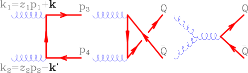
Figure 2: Diagrams for heavy quark hadroproduction

In the large centre of mass energy limit the perturbative expansion of the short-distance cross section contains large terms of order $\alpha_{s}^{3}[\alpha_{s}(M^{2})\log(s/M^{2})]^{n}$ which need to be resummed to all orders. This resummation is performed by using the ${\mathbf{k}}$-factorized expression for the cross section, which here takes the form

$$\Sigma(\rho) = \sum_{ij}\int\;\frac{dz_{1}}{z_{1}}\frac{dz_{2}}{z_{2}}\frac{d^{2}{\mathbf{k}}}{\pi}\frac{d^{2}{\mathbf{k}}^{\prime}}{\pi}\;\hat{\Sigma}_{ij}({\mathbf{k}},{\mathbf{k}}^{\prime},M^{2},z_{1}z_{2}s)\;\mathcal{F}^{i}(z_{1},{\mathbf{k}}^{2},\mu^{2})\times$$ (46)

$$\hphantom{\sum_{ij}\int\;}\!\times\,\mathcal{F}^{j}(z_{2},{\mathbf{k}}^{\prime\;2},\mu^{2})\,,$$

in which $\mathcal{F}_{i}$ are the unintegrated parton distribution functions and $\hat{\Sigma}$ is the (lowest-order and gauge-invariant) off-shell continuation of the parton cross section. Taking Mellin moments with respect to the longitudinal momenta (see eqs. (9) and (43)) again undoes the convolution:

$$\Sigma_{\omega}=\sum_{ij}\int\;\frac{d^{2}{\mathbf{k}}}{\pi}\frac{d^{2}{\mathbf{k}}^{\prime}}{\pi}\;H^{ij}_{\omega}\left(\frac{\mathbf{k}}{M},\frac{{\mathbf{k}}^{\prime}}{M}\right)\;\mathcal{F}^{i}_{\omega}({\mathbf{k}}^{2},\mu^{2})\mathcal{F}^{j}_{\omega}({\mathbf{k}}^{\prime\;2},\mu^{2})\,.$$ (47)

A further simplification is obtained by Mellin transform with respect to the transverse momenta:

$$\Sigma_{\omega}=\sum_{ij}\int_{C}\frac{d\gamma_{1}d\gamma_{2}}{(2\pi i)^{2}}\left(\frac{M^{2}}{\mu^{2}}\right)^{\gamma_{1}+\gamma_{2}}\mathcal{F}^{i}_{\omega}(\gamma_{1})\;\mathcal{F}^{j}_{\omega}(\gamma_{2})\;H^{ij}_{\omega}(\gamma_{1},\gamma_{2})\,,$$ (48)

where the Mellin transforms of the unintegrated parton distribution functions are defined as in eq. (15) and the impact factor

$$H^{ij}_{\omega}(\gamma_{1},\gamma_{2})=\int_{0}^{\infty}\frac{d^{2}{\mathbf{k}}}{\pi{\mathbf{k}}^{2}}\frac{d^{2}{\mathbf{k}}^{\prime}}{\pi{\mathbf{k}}^{\prime 2}}\left(\frac{{\mathbf{k}}^{2}}{M^{2}}\right)^{\gamma_{1}}\left(\frac{{\mathbf{k}}^{\prime 2}}{M^{2}}\right)^{\gamma_{2}}H^{ij}_{\omega}\left(\frac{\mathbf{k}}{M},\frac{{\mathbf{k}}^{\prime}}{M}\right).$$ (49)

When we pick up the residues of the two perturbative poles eq. (19) in the $\gamma_{1}$, $\gamma_{2}$ integrations, we find in a sequence of steps analogous to those leading to eq. (25)

$$\Sigma_{\omega}=\sum_{ij}\left(\gamma_{s}\left(\frac{a}{\omega}\right)\right)^{2}H^{ij}_{\omega}\left(\gamma_{s}\left(\frac{a}{\omega}\right),\gamma_{s}\left(\frac{a}{\omega}\right)\right)\left(\frac{M^{2}}{\mu^{2}}\right)^{2\gamma_{s}(a/\omega)}\;F^{i}_{\omega}(\mu^{2})\;F^{j}_{\omega}(\mu^{2})\,,$$ (50)

where $F^{i}_{\omega}(\mu^{2})$ are the integrated parton distribution functions at scale $\mu^{2}$.

It thus remains to determine the impact factors $H^{ij}_{\omega}(\gamma_{1},\gamma_{2})$. This requires the calculation of the moments of the heavy quark production cross section with two incoming off shell gluons. Details of this calculation may be found in the appendix. The answer in our normalization, and for $\omega=0$, is

$$H_{0}(\gamma_{1},\gamma_{2}) = \frac{\pi\alpha_{S}^{2}}{V_{c}}B(\gamma_{1},1-\gamma_{1})B(\gamma_{2},1-\gamma_{2})\times$$

$$\times\left\{4N_{c}\;\left[\frac{B(3-\gamma_{1}-\gamma_{2},3-\gamma_{1}-\gamma_{2})}{(1-\gamma_{1}-\gamma_{2})}\right.\right.+$$

$$\hphantom{\times\Bigg{\{}4N_{c}\;\Bigg{[}}\!\left.+\,\frac{B(3-\gamma_{1}-\gamma_{2},3-\gamma_{1}-\gamma_{2})}{(1-\gamma_{1}-\gamma_{2})^{3}\;B^{2}(1-\gamma_{1},1-\gamma_{2})}\right]-$$

$$\hphantom{\times\Bigg{\{}}\!\left.-\,\frac{2}{N_{c}}\frac{\Gamma(2-\gamma_{1})\Gamma(2-\gamma_{2})\Gamma(2-\gamma_{1}-\gamma_{2})}{\Gamma(4-2\gamma_{1})\Gamma(4-2\gamma_{2})}\frac{(7-5(\gamma_{1}+\gamma_{2})+3\gamma_{1}\gamma_{2})}{(1-\gamma_{1}-\gamma_{2})}\right\}.$$

This calculation has previously been reported in [20, 21]. Note that eq. (3.2) is in disagreement with ref. [20, eq. (2.10)] and ref. [21, eqs. (3.14)].

When $\omega=0$ $H_{\omega}(\gamma_{1},\gamma_{2})$ has a triple pole at $\gamma_{1}=1-\gamma_{2}$, which splits into a simple and a double pole when $\omega$ is non zero. In the vicinity of $\gamma_{1}=\gamma_{2}=1/2$ one finds the singularity structure [18]

$$\gamma_{1}\gamma_{2}H_{\omega}(\gamma_{1},\gamma_{2})=\frac{\pi\alpha_{S}^{2}}{V_{c}}\;\frac{N_{c}}{6}\;\frac{1}{(1-\gamma_{1}-\gamma_{2})}\frac{1}{(1-\gamma_{1}-\gamma_{2}+\omega)^{2}}\,.$$ (52)

This singularity comes from the propagator for the $s$-channel gluon in the third diagram in figure 2: it is thus intrinsically non abelian, in the sense that it is not present in the high energy direct photoproduction cross-section given by the diagrams of figure 1. The singularity can drive a substantial rise in the hadroproduction cross-section at high energies, as we will show in detail in the next section.

Since away from these singularities $H_{\omega}(\gamma_{1},\gamma_{2})$ is regular in $\omega$, we may write

$$\gamma_{1}\gamma_{2}H_{\omega}(\gamma_{1},\gamma_{2})=h(\gamma_{1},\gamma_{2})+O(\omega)\,.$$ (53)

In the perturbative limit for small $\gamma_{1}$ and $\gamma_{2}$ we then have

$$h(\gamma_{1},\gamma_{2})\sim\frac{\pi\alpha_{s}^{2}}{V_{c}}\left[\frac{4}{15}N_{c}-\frac{7}{18}\frac{1}{N_{c}}+(\gamma_{1}+\gamma_{2})\left(\frac{154}{225}N_{c}-\frac{41}{54}\frac{1}{N_{c}}\right)+\cdots\right],$$ (54)

so that

$$h(0,0) = \frac{\pi\alpha_{s}^{2}}{V_{c}}\left(\frac{4}{15}N_{c}-\frac{7}{18}\frac{1}{N_{c}}\right),$$ (55)

$$\frac{d}{d\gamma}h(\gamma,0)\Big{|}_{\gamma=0} \equiv h^{\prime}(0,0)=\frac{\pi\alpha_{s}^{2}}{V_{c}}\left(\frac{154}{225}N_{c}-\frac{41}{54}\frac{1}{N_{c}}\right).$$ (56)

As in the photoproduction case we must take care to identify the factorization scheme correctly. In particular to change eq. (3.2) from the “$k_{T}$-factorization scheme” to $\overline{\mathrm{MS}}$ factorization now introduces a factor of $R(\gamma_{1})R(\gamma_{2})$, with $R$ the $\overline{\mathrm{MS}}$-gluon normalization factor eq. (31), so that in $\overline{\mathrm{MS}}$

$$\gamma_{1}\gamma_{2}H^{gg}_{\omega}(\gamma_{1},\gamma_{2})=h(\gamma_{1},\gamma_{2})R(\gamma_{1})R(\gamma_{2})+O(\omega)\,.$$ (57)

Furthermore arguments similar to those in ref. [43] may again be used to determine LLx high energy heavy quark production cross sections with incoming quarks in terms of those with incoming gluons: again in $\overline{\mathrm{MS}}$ (compare eq. (36))

$$\gamma_{1}\gamma_{2}H^{gq}_{\omega}(\gamma_{1},\gamma_{2}) = r_{c}(h(\gamma_{1},\gamma_{2})R(\gamma_{1})R(\gamma_{2})-h(\gamma_{1},0)R(\gamma_{1}))+O(\omega)\,,$$

$$\gamma_{1}\gamma_{2}H^{qq}_{\omega}(\gamma_{1},\gamma_{2}) = r_{c}\left(h(\gamma_{1},\gamma_{2})R(\gamma_{1})R(\gamma_{2})-h(\gamma_{1},0)R(\gamma_{1})\right.-$$ (58)

$$\hphantom{r_{c}\Bigg{(}}\!\left.-\,h(0,\gamma_{2})R(\gamma_{2})+h(0,0)\right)+O(\omega)\,,$$

and similarly for the various other combinations.

Putting all this together, in the high energy limit the partonic cross sections for hadroproduction of heavy quarks are

$$\hat{\Sigma}^{gg}_{\omega} = h\left(\gamma_{s}\left(\frac{a}{\omega}\right),\gamma_{s}\left(\frac{a}{\omega}\right)\right)R^{2}\left(\gamma_{s}\left(\frac{a}{\omega}\right)\right)\left(\frac{M^{2}}{\mu^{2}}\right)^{2\gamma_{s}(a/\omega)},$$

$$\hat{\Sigma}^{gq}_{\omega} = \hat{\Sigma}^{g\bar{q}}_{\omega}=r_{c}\left[h\left(\gamma_{s}\left(\frac{a}{\omega}\right),\gamma_{s}\left(\frac{a}{\omega}\right)\right)R^{2}\left(\gamma_{s}\left(\frac{a}{\omega}\right)\right)\left(\frac{M^{2}}{\mu^{2}}\right)^{2\gamma_{s}(a/\omega)}\right.-$$

$$\hphantom{\hat{\Sigma}^{g\bar{q}}_{\omega}=r_{c}\Bigg{[}}\!\left.-\,h\left(\gamma_{s}\left(\frac{a}{\omega}\right),0\right)R\left(\gamma_{s}\left(\frac{a}{\omega}\right)\right)\left(\frac{M^{2}}{\mu^{2}}\right)^{\gamma_{s}(a/\omega)}\right],$$

$$\hat{\Sigma}^{q\bar{q}}_{\omega} = \hat{\Sigma}^{\bar{q}q}_{\omega}=\hat{\Sigma}^{qq}_{\omega}=\hat{\Sigma}^{\bar{q}\bar{q}}_{\omega}=r_{c}^{2}\left[h\left(\gamma_{s}\left(\frac{a}{\omega}\right),\gamma_{s}\left(\frac{a}{\omega}\right)\right)R^{2}\left(\gamma_{s}\left(\frac{a}{\omega}\right)\right)\left(\frac{M^{2}}{\mu^{2}}\right)^{2\gamma_{s}(a/\omega)}\right.-$$ (59)

$$\hphantom{\hat{\Sigma}^{\bar{q}q}_{\omega}=\hat{\Sigma}^{qq}_{\omega}=\hat{\Sigma}^{\bar{q}\bar{q}}_{\omega}=r_{c}^{2}\Bigg{[}}\!-\,2h\left(\gamma_{s}\left(\frac{a}{\omega}\right),0\right)R\left(\gamma_{s}\left(\frac{a}{\omega}\right)\right)\left(\frac{M^{2}}{\mu^{2}}\right)^{\gamma_{s}(a/\omega)}+$$

$$\hphantom{\hat{\Sigma}^{\bar{q}q}_{\omega}=\hat{\Sigma}^{qq}_{\omega}=\hat{\Sigma}^{\bar{q}\bar{q}}_{\omega}=r_{c}^{2}\Bigg{[}}\!\left.+\,h(0,0)\vphantom{\left(\frac{M^{2}}{\mu^{2}}\right)^{\gamma_{s}(a/\omega)}}\right].$$

3.3 Double leading resummation

The perturbative expansion of the $\overline{\mathrm{MS}}$ partonic cross-sections eqs. (59) may be derived using eqs. (21), (32) and (54):

$$h\left(\gamma_{s}\left(\frac{a}{\omega}\right),\gamma_{s}\left(\frac{a}{\omega}\right)\right)R^{2}\left(\gamma_{s}\left(\frac{a}{\omega}\right)\right) \sim h(0,0)+2\frac{a}{\omega}h^{\prime}(0,0)+O\left(\alpha_{s}^{2}\left(\frac{a}{\omega}\right)^{2}\right),$$

$$h\left(\gamma_{s}\left(\frac{a}{\omega}\right),0\right)R\left(\gamma_{s}\left(\frac{a}{\omega}\right)\right) \sim h(0,0)+\frac{a}{\omega}h^{\prime}(0,0)+O\left(\alpha_{s}^{2}\left(\frac{a}{\omega}\right)^{2}\right),\qquad$$ (60)

with $h(0,0)$ and $h^{\prime}(0,0)$ given by eqs. (55) and (56), consistent with the fixed order results eqs. (45). Combining the fixed order cross-sections with the high energy cross-sections, taking care to subtract the terms eqs. (45) to avoid double counting, we get

$$\hat{\Sigma}^{gg}_{\omega} = \alpha_{s}^{2}\left\{f_{gg\;\omega}^{(0)}+4\pi\alpha_{s}\left[f_{gg\;\omega}^{(1)}+\ln\left(\frac{\mu^{2}}{M^{2}}\right)\bar{f}_{gg\;\omega}^{(1)}\right]\right\}+$$

$$+\,\left[h\left(\gamma_{s}\left(\frac{a}{\omega}\right),\gamma_{s}\left(\frac{a}{\omega}\right)\right)R^{2}\left(\gamma_{s}\left(\frac{a}{\omega}\right)\right)\left(\frac{M^{2}}{\mu^{2}}\right)^{2\gamma_{s}(a/\omega)}\right.-$$

$$\hphantom{+\,\Bigg{[}}\!\left.-\,h(0,0)\left(1+2\frac{a}{\omega}\ln\frac{M^{2}}{\mu^{2}}\right)-2\frac{a}{\omega}h^{\prime}(0,0)\right],$$

$$\hat{\Sigma}^{gq}_{\omega} = \hat{\Sigma}^{g\bar{q}}_{\omega}=\alpha_{s}^{2}\left\{4\pi\alpha_{s}\left[f_{gq\;\omega}^{(1)}+\ln\left(\frac{\mu^{2}}{M^{2}}\right)\bar{f}_{gq\;\omega}^{(1)}\right]\right\}+$$

$$\hphantom{\hat{\Sigma}^{g\bar{q}}_{\omega}=}\!+\,r_{c}\left[h\left(\gamma_{s}\left(\frac{a}{\omega}\right),\gamma_{s}\left(\frac{a}{\omega}\right)\right)R^{2}\left(\gamma_{s}\left(\frac{a}{\omega}\right)\right)\left(\frac{M^{2}}{\mu^{2}}\right)^{2\gamma_{s}(a/\omega)}\right.-$$

$$\hphantom{\hat{\Sigma}^{g\bar{q}}_{\omega}=+\,r_{c}\Bigg{[}}\!-\,h\left(\gamma_{s}\left(\frac{a}{\omega}\right),0\right)R\left(\gamma_{s}\left(\frac{a}{\omega}\right)\right)\left(\frac{M^{2}}{\mu^{2}}\right)^{\gamma_{s}(a/\omega)}-$$

$$\hphantom{\hat{\Sigma}^{g\bar{q}}_{\omega}=+\,r_{c}\Bigg{[}}\!\left.-\,h(0,0)\frac{a}{\omega}\ln\frac{M^{2}}{\mu^{2}}-\frac{a}{\omega}h^{\prime}(0,0)\vphantom{\left(\frac{M^{2}}{\mu^{2}}\right)^{2\gamma_{s}(a/\omega)}}\right],$$

$$\hat{\Sigma}^{q\bar{q}}_{\omega} = \hat{\Sigma}^{\bar{q}q}_{\omega}=\alpha_{s}^{2}\left\{f_{q\bar{q}\;\omega}^{(0)}+4\pi\alpha_{s}\left[f_{q\bar{q}\;\omega}^{(1)}+\ln\left(\frac{\mu^{2}}{M^{2}}\right)\bar{f}_{q\bar{q}\;\omega}^{(1)}\right]\right\}+$$

$$\hphantom{\hat{\Sigma}^{\bar{q}q}_{\omega}=}\!+\,r_{c}^{2}\left[h\left(\gamma_{s}\left(\frac{a}{\omega}\right),\gamma_{s}\left(\frac{a}{\omega}\right)\right)R^{2}\left(\gamma_{s}\left(\frac{a}{\omega}\right)\right)\left(\frac{M^{2}}{\mu^{2}}\right)^{2\gamma_{s}(a/\omega)}\right.-$$

$$\hphantom{\hat{\Sigma}^{\bar{q}q}_{\omega}=+\,r_{c}^{2}\Bigg{[}}\!\left.-\,2h\left(\gamma_{s}\left(\frac{a}{\omega}\right),0\right)R\left(\gamma_{s}\left(\frac{a}{\omega}\right)\right)\left(\frac{M^{2}}{\mu^{2}}\right)^{\gamma_{s}(a/\omega)}+h(0,0)\right],$$

$$\hat{\Sigma}^{qq}_{\omega} = \hat{\Sigma}^{\bar{q}\bar{q}}_{\omega}=r_{c}^{2}\left[h\left(\gamma_{s}\left(\frac{a}{\omega}\right),\gamma_{s}\left(\frac{a}{\omega}\right)\right)R^{2}\left(\gamma_{s}\left(\frac{a}{\omega}\right)\right)\left(\frac{M^{2}}{\mu^{2}}\right)^{2\gamma_{s}(a/\omega)}\right.-$$ (61)

$$\hphantom{\hat{\Sigma}^{\bar{q}\bar{q}}_{\omega}=r_{c}^{2}\Bigg{[}}\!\left.-\,2h\left(\gamma_{s}\left(\frac{a}{\omega}\right),0\right)R\left(\gamma_{s}\left(\frac{a}{\omega}\right)\right)\left(\frac{M^{2}}{\mu^{2}}\right)^{\gamma_{s}(a/\omega)}+h(0,0)\right].$$

The NLLx resummation [39] may be implemented just as in the photoproduction case, with similar ambiguities in the treatment of the double counting terms: here this ambiguity should be relatively unimportant at high energies since it has no effect on the singularities of $h(\gamma_{s}(a/\omega),\gamma_{s}(a/\omega))$.

4 Asymptotic behaviour at high energy

The aim of this paper has been to calculate and collect results so that a matched numerical calculation of heavy quark cross sections is possible. The matching is necessary so that the calculation correctly includes the known fixed order results as well as the leading tower of logarithms present at high energy.

In the following we give some analytic results for the high energy resummation alone; these are in no way meant to supplant the complete analysis alluded to above, but instead serve to indicate some features of the high energy resummation. First, we will obtain results for the asymptotic behaviour of the gluon distribution function at high energy, keeping the coupling fixed. We consider two alternative choices for the anomalous dimension: an anomalous dimension given simply by the singular term in lowest order perturbation theory (so that $\chi\sim 1/\gamma$ and has no minimum) and, for contrast, the lowest order BFKL anomalous dimension (so that the corresponding $\chi$-function has a minimum at $\gamma=1/2$). Second, we will explore the consequences of these two forms of the anomalous dimension for the high energy behaviour of the heavy quark photoproduction and hadroproduction cross sections, expressing the results in terms of the integrated gluon distribution function. For simplicity, only the gluon contributions will be considered, since the quark contributions are smaller. Last, we will attempt a more quantitative estimate of the expected enhancement by letting the coupling run and choosing $\gamma=a(\frac{1}{\omega}-1)$, so that $\chi(\gamma)=1/(\gamma+a)$ and the momentum conservation constraint at $\omega=1$ is satisfied explicitly. This form is a good approximation to the fully resummed anomalous dimension [37, 38, 39] and furthermore gives a good account of scaling violations in HERA structure function data [24].

4.1 Gluon distribution

In $x$ space, the integrated gluon distribution at the heavy quark mass scale, $M$, can be obtained by performing the inverse Mellin transform of eq. (24) with respect to $\omega$

$$G(x,M^{2}) = \int_{C}\frac{d\omega}{2\pi i}\;x^{-\omega}\left(\frac{M^{2}}{\mu_{0}^{2}}\right)^{\gamma_{s}(a/\omega)}G^{0}(\omega)$$ (62)

$$= \int_{C}\frac{d\omega}{(2\pi i)}\exp{\left(\omega L_{x}+\gamma_{s}\left(\frac{a}{\omega}\right)l\right)}G^{0}(\omega)\,,$$

where $L_{x}=\ln(1/x)$, $l=\ln(M^{2}/\mu_{0}^{2})$. Here $G^{0}(\omega)\equiv F^{g}_{\omega}(\mu_{0}^{2})$ is a starting function at scale $\mu_{0}$ which we will assume is benign in terms of poles. For simplicity, we will work entirely in the “$k_{T}$-factorization scheme”, so that the factors of $R$ (see eq. (31)) are absorbed into the gluon distribution.

The asymptotic form of $G(x,M^{2})$ depends on the form of the singular anomalous dimension $\gamma_{s}(a/\omega)$. If we take the simple form $\gamma_{s}(a/\omega)=a/\omega$, the $\omega$ integration may be done by a saddle point approximation [44], with the result

$$G(x,M^{2})\simeq\frac{(al)^{1/4}}{(4\pi)^{1/2}L_{x}^{3/4}}\exp\left(2\sqrt{alL_{x}}\right)G^{0}\left(\sqrt{\frac{al}{L_{x}}}\right),$$ (63)

where the argument of $G^{0}$ is the position of the saddle point.

If, on the other hand, the anomalous dimension $\gamma_{s}(a/\omega)$ is more like the BFKL form, it is convenient to make the usual change of variables $\omega\>\>\!=\>\>\!a\chi(\gamma)$, (see eq. (20)),

$$G(x,M^{2})=\int_{C}\frac{d\gamma}{2\pi i}(-a\chi^{\prime}(\gamma))\;\exp{\left(a\chi(\gamma)L_{x}+\gamma l\right)}\;G^{0}(a\chi(\gamma))\,.$$ (64)

If we now specialize to a $\chi$-function which has a minimum at one half

$$\chi(\gamma)\approx\chi\left(\frac{1}{2}\right)+\frac{1}{2}\chi^{\prime\prime}\left(\frac{1}{2}\right)\left(\gamma-\frac{1}{2}\right)^{2}+\cdots\,,$$ (65)

so that, as $L_{x}$ increases, the saddle point in the $\gamma$ integration moves to $1/2$ from below. Asymptotically we then find when $L_{x}\gg l$

$$G(x,M^{2})\sim\frac{l\;L_{x}^{-3/2}}{(2\pi a\chi^{\prime\prime}(1/2))^{1/2}}\exp\left(aL_{x}\chi\left(\frac{1}{2}\right)+\frac{1}{2}l\right)G^{0}\left(a\chi\left(\frac{1}{2}\right)\right).$$ (66)

Now consider the direct component of the photoproduction cross-section in the high energy limit. From eq. (25) we have that

$$\Sigma(\rho)=\int_{C}\frac{d\omega}{(2\pi i)}\exp{\left(\omega L+\gamma_{s}\left(\frac{a}{\omega}\right)l\right)}j\left(\gamma_{s}\left(\frac{a}{\omega}\right)\right)G^{0}(\omega)\,,$$ (67)

where $L\equiv\ln 1/\rho$. The function $j(\gamma)$, defined in eq. (28) is free from poles in the interval $0<\gamma<1$ and is therefore a smooth function in the region of the saddle points of the integrand. It follows that at high energy for the “perturbative” gluon, eq. (63),

$$\Sigma(\rho) \simeq \frac{(al)^{1/4}}{(4\pi)^{1/2}L^{3/4}}\exp\left(2\sqrt{alL}\right)\;j\left(\frac{a}{\overline{\omega}}\right)\;G^{0}(\overline{\omega})$$ (68)

$$\simeq j\left(\frac{a}{\overline{\omega}}\right)\;G(\rho,M^{2})\,,$$

where $\overline{\omega}=\sqrt{al/L}$ is the position of the saddle point. This expression will break down when the argument of $j$ approaches one, since $j$ has a simple pole there, but should still be good around $a/\overline{\omega}\sim 1/2$, where it leads to a small enhancement [18]. For the BFKL gluon, eq. (66), we find at high energy

$$\Sigma(\rho)\simeq j\left(\frac{1}{2}\right)G(\rho,M^{2})\,.$$ (69)

In both cases the rise in the gluon drives the rise in the cross-section, with only a modest enhancement over the leading order result, $j(0)G(\rho,M^{2})$.

4.2 Hadroproduction

We now consider the high energy behaviour of the cross section for the hadroproduction of a pair of quarks of mass $M$. From eq. (50) we have

$$\Sigma(\rho) = \int_{C}\frac{d\omega}{(2\pi i)}\rho^{-\omega}\;\left(\gamma_{s}\left(\frac{a}{\omega}\right)\right)^{2}H_{\omega}\left(\gamma_{s}\left(\frac{a}{\omega}\right),\gamma_{s}\left(\frac{a}{\omega}\right)\right)\left(\frac{M^{2}}{\mu_{0}^{2}}\right)^{2\gamma_{s}(a/\omega)}\left[G^{0}(\omega)\right]^{2}$$ (70)

$$= \int_{C}\frac{d\omega}{(2\pi i)}\exp{\left(\omega L+2\gamma_{s}\left(\frac{a}{\omega}\right)l\right)}\;h_{\omega}\left(\gamma_{s}\left(\frac{a}{\omega}\right),\gamma_{s}\left(\frac{a}{\omega}\right)\right)\left[G^{0}(\omega)\right]^{2}$$

$$= \int_{C}\frac{d\gamma}{2\pi i}(-a\chi^{\prime}(\gamma))\;\exp{\left(a\chi(\gamma)L+2\gamma l\right)}h_{\omega}\left(\gamma,\gamma\right)\left[G^{0}(a\chi(\gamma))\right]^{2},$$

where $h_{\omega}(\gamma,\gamma)=\gamma^{2}H_{\omega}(\gamma,\gamma)$, $L\equiv\ln 1/\rho$ and in the last line we again made the change of variables $\omega=a\chi(\gamma)$. In contrast to the direct photoproduction cross-section considered above, the asymptotic behaviour at large $L$ will now be dominated by the singularities of $h_{\omega}(\gamma_{1},\gamma_{2})$ (see eq. (52)),

$$h_{\omega}(\gamma,\gamma) \simeq \frac{A}{(1-2\gamma)(1-2\gamma+\omega)^{2}}$$ (71)

$$= \frac{A}{\omega^{2}}\left[\frac{1}{(1-2\gamma)}-\frac{1}{(1-2\gamma+\omega)}-\frac{\omega}{(1-2\gamma+\omega)^{2}}\right]$$

with $A=\pi\alpha_{s}^{2}\frac{N_{c}}{6V_{c}}$.

First consider the “perturbative” anomalous dimension $\gamma=a/\omega$. Because the behaviour in $\omega$ is more intuitive we choose to work with the $\omega$ representation, eq. (70). With this choice for $\gamma$, eq. (71) becomes

$$h_{\omega}\left(\frac{a}{\omega},\frac{a}{\omega}\right) \equiv A\;f(\omega,\omega_{0},\omega_{+},\omega_{-})$$ (72)

$$= A\left[-\frac{1}{\omega_{+}\omega_{-}(\omega-\omega_{0})}-\frac{1}{(\omega_{+}-\omega_{-})^{2}}\left\{\frac{\omega_{+}}{(\omega-\omega_{+})^{2}}+\frac{\omega_{-}}{(\omega-\omega_{-})^{2}}\right\}\right.-$$

$$\hphantom{A\Bigg{[}}\!\left.-\frac{1}{(\omega_{+}-\omega_{-})^{3}}\left\{\frac{(\omega_{-}^{2}-3\omega_{-}\omega_{+})}{\omega_{+}(\omega-\omega_{+})}+\frac{(3\omega_{-}\omega_{+}-\omega_{+}^{2})}{\omega_{-}(\omega-\omega_{-})}\right\}\right],$$

where

$$\omega_{0}=2a\,,\qquad\omega_{\pm}=\frac{[-1\pm\sqrt{1+8a}]}{2}\,.$$ (73)

The dominant behaviour at large $L$ and $l$ depends on the position of the saddle point, $\overline{\omega}=\sqrt{2al/L}$ relative to the rightmost pole, $\omega=\omega_{0}$. If the saddle point is to the right of the pole, $\overline{\omega}>2a$, (which means $2aL<l$), we integrate along the contour $\omega=\overline{\omega}+iz$ to obtain the result

$$\Sigma(\rho) \simeq \frac{A}{2\pi}\exp{\left(\overline{\omega}L+2\frac{a}{\overline{\omega}}l\right)}\;\left[G^{0}(\overline{\omega})\right]^{2}\int_{-\infty}^{\infty}dz\;f(\overline{\omega}+iz,\omega_{0},\omega_{+},\omega_{-})\times$$ (74)

$$\hphantom{\frac{A}{2\pi}\exp{\left(\overline{\omega}L+2\frac{a}{\overline{\omega}}l\right)}\;\left[G^{0}(\overline{\omega})\right]^{2}\int_{-\infty}^{\infty}}\!\times\,\exp\left(-\frac{z^{2}}{c^{2}}\right),$$

where $f$ is given in eq. (72) and the quantity $c$,

$$c=\left({\frac{\overline{\omega}^{3}}{2al}}\right)^{1/2}$$ (75)

sets the scale of the gaussian fluctuations which determines whether the poles at $\omega_{0},\omega_{+}$ and $\omega_{-}$ should be considered close.

Using the saddle point method in the vicinity of poles we need to consider integrals of the general form

$$K_{n}(y)=c^{n-1}\int_{-\infty}^{\infty}dz\frac{1}{(b+iz)^{n}}\exp\left(-\frac{z^{2}}{c^{2}}\right),$$ (76)

with $y=b/c$ and $b,c\neq 0$: $K_{n}(-y)=(-)^{n}K_{n}(y)$. An evaluation of the first three of these integrals $K_{1}(y)$, $K_{2}(y)$ and $K_{3}(y)$ may be found in the appendix B. In terms of these functions the result is

$$\Sigma(\rho)=\frac{Ac}{(4\pi)^{1/2}}\;X(\overline{\omega},\omega_{0},\omega_{+},\omega_{-})\;\exp\big{(}2\sqrt{2alL}\big{)}\;[G^{0}(\overline{\omega})]^{2}\,,$$ (77)

where

$$X(\overline{\omega},\omega_{0},\omega_{+},\omega_{-}) = \frac{1}{c\sqrt{\pi}}\int_{-\infty}^{\infty}dz\;f(\overline{\omega}+iz,\omega_{0},\omega_{+},\omega_{-})\exp\left(-\frac{z^{2}}{c^{2}}\right)$$ (78)

$$= \frac{1}{c\sqrt{\pi}}\left[-\frac{1}{\omega_{+}\omega_{-}}K_{1}\left(\frac{(\overline{\omega}-\omega_{0})}{c}\right)\right.-$$

$$\hphantom{\frac{1}{c\sqrt{\pi}}\Bigg{[}}\!-\,K_{1}\left(\frac{(\overline{\omega}-\omega_{+})}{c}\right)\frac{\omega_{-}(\omega_{-}-3\omega_{+})}{\omega_{+}(\omega_{+}-\omega_{-})^{3}}-$$

$$\hphantom{\frac{1}{c\sqrt{\pi}}\Bigg{[}}\!-\,K_{2}\left(\frac{(\overline{\omega}-\omega_{+})}{c}\right)\frac{\omega_{+}}{c(\omega_{+}-\omega_{-})^{2}}+$$

$$\hphantom{\frac{1}{c\sqrt{\pi}}\Bigg{[}}\!+\,K_{1}\left(\frac{(\overline{\omega}-\omega_{-})}{c}\right)\frac{\omega_{+}(\omega_{+}-3\omega_{-})}{\omega_{-}(\omega_{+}-\omega_{-})^{3}}-$$

$$\hphantom{\frac{1}{c\sqrt{\pi}}\Bigg{[}}\!\left.-\,K_{2}\left(\frac{(\overline{\omega}-\omega_{-})}{c}\right)\frac{\omega_{-}}{c(\omega_{+}-\omega_{-})^{2}}\right].$$

Expressed in terms of the gluon distribution eq. (63), we find

$$\Sigma(\rho)\simeq A\frac{\pi^{1/2}L^{3/4}}{(2al)^{1/4}}\;X(\overline{\omega},\omega_{0},\omega_{+},\omega_{-})\;\left[G(\sqrt{\rho},M^{2})\right]^{2},$$ (79)

where we have used the fact that if $x=\sqrt{\rho}$, $L_{x}=\frac{1}{2}L$ and thus $2\sqrt{2alL}=4\sqrt{2alL_{x}}$. As $\overline{\omega}\rightarrow\omega_{0}$ from above, the enhancement factor $X(\overline{\omega},\omega_{0},\omega_{+},\omega_{-})$ grows until it reaches a maximum value at the pole.

When $\overline{\omega}$ passes the pole, we have to add the residue of the pole to the saddle contribution. The result for the pole contribution for $2aL>l$ is

$$\Sigma(\rho) \simeq \frac{A}{2a}\exp\left(2aL+l\right)\;[G^{0}(\omega_{0})]^{2}$$ (80)

$$\simeq A\frac{\pi l}{4a^{3}}\exp\left(2aL-l\right)\;[G(e^{-l/4a},M^{2})]^{2}\,.$$

At high energies this contribution is dominant, since it grows as $e^{2aL}=\rho^{-2a}$. Taken at face value, eq. (80) thus indicates a dramatic growth of the hadroproduction cross-section with increasing energy, driven not by the growth of the gluon distributions but rather by the perturbative singularity in the partonic cross-section.

If instead we consider the BFKL anomalous dimension, the asymptotic behaviour of the hadroproduction cross-section is best determined using the $\gamma$-representation, eq. (70) and $h_{\omega}$ as given by eq. (71), The function $\chi(\gamma)$, eq. (65), has a minimum at $\gamma=1/2$, and $\Sigma$ is thus approximately given by

$$\simeq\frac{aA\chi^{\prime\prime}(1/2)}{8}\int_{C}\frac{d\gamma}{2\pi i}\;\frac{\exp{\left(a\chi(\gamma)L+2\gamma l\right)}}{(\gamma-\frac{1}{2}-\frac{1}{2}a\chi(1/2))^{2}}\;[G^{0}(a\chi(\gamma))]^{2}\,.$$ (81)

The integrand now has a saddle point at

$$\overline{\gamma}=\frac{1}{2}-\frac{2l}{aL\chi^{\prime\prime}(1/2)}\,,$$ (82)

and the fluctuations about the saddle are determined by $c_{\gamma}=\sqrt{2/(a\chi^{\prime\prime}L)}$. The saddle point is always to the left of $1/2$ which it approaches asymptotically as $L$ increases. The double pole is at a fixed distance to the right of $1/2$. The behaviour at large $L$ is thus given by

$$\Sigma(\rho) \simeq \frac{aA\sqrt{\chi^{\prime\prime}(1/2)}}{16\pi c_{\gamma}}K_{2}\left(\frac{a\chi(1/2)}{2c_{\gamma}}\right)\exp{\left(a\chi\left(\frac{1}{2}\right)L+l\right)}\left[G^{0}\left(a\chi\left(\frac{1}{2}\right)\right)\right]^{2}$$ (83)

$$\simeq \frac{A\sqrt{\chi^{\prime\prime}(1/2)}}{2a[\chi(1/2)]^{2}\sqrt{2\pi aL}}\exp{\left(a\chi\left(\frac{1}{2}\right)L+l\right)}\;\left[G^{0}\left(a\chi\left(\frac{1}{2}\right)\right)\right]^{2}$$

which when expressed in terms of the BFKL gluon eq. (66) becomes

$$\Sigma(\rho)\simeq\frac{A}{16}\sqrt{\frac{2\pi}{a\chi^{\prime\prime}(1/2)}}\left(\frac{\chi^{\prime\prime}(1/2)}{\chi(1/2)}\right)^{2}\frac{L^{5/2}}{l^{2}}\left[G(\sqrt{\rho},M^{2})\right]^{2}.$$ (84)

Clearly in the BFKL case, although there is some enhancement [18], it is rather less dramatic than in the previous case. This is because when $\chi(\gamma)$ has a minimum, the saddle point cannot travel past the pole at $\gamma=1/2$.

In summary, because of the singularity structure of eq. (52) substantial enhancements of the hadroproduction cross-section are possible at high energy, even when the gluon distribution function does not have the singular behaviour predicted by lowest order BFKL.

4.3 A more realistic model

In order to attempt a quantitative estimate of the enhancement in the hadroproduction cross-section at the Tevatron and LHC, we take a simple model for the anomalous dimension function which is close to the one-loop value and satisfies momentum conservation,

$$\gamma(\omega)=a\left(\frac{1}{\omega}-1\right).$$ (85)

We also include running coupling effects. In a theory with a running coupling the product $la$ is replaced by

$$\zeta(\mu)=\frac{N_{c}}{\pi}\int_{\mu_{0}^{2}}^{\mu^{2}}\frac{dk^{2}}{k^{2}}\alpha_{S}(k^{2})=\frac{N_{c}}{\pi b_{0}}\ln\left(\frac{\ln(\mu^{2}/\Lambda^{2})}{\ln(\mu_{0}^{2}/\Lambda^{2})}\right).$$ (86)

If we take the leading order parameter $\Lambda=200\,\mbox{MeV}$ (corresponding to the leading order coupling at the $Z$-mass $\alpha_{s}(M_{z})=0.123$), we find that $a=0.224$. Further, taking $\mu_{0}=1\,\mbox{GeV}$ from eq. (86) we find $\zeta(M)\simeq 1$. We shall adopt this value in our numerical estimates below, although the details will change if we use different values for $\mu_{0}$ and $\Lambda$.

The modified anomalous dimension, eq. (85), only changes eq. (63) in a minor way

$$G(x,\mu^{2})=\frac{(\zeta(\mu))^{1/4}}{(4\pi)^{1/2}L_{x}^{3/4}}\exp\left[2\sqrt{\zeta(\mu)L_{x}}-\zeta(\mu)\right]\;G^{0}\left(\sqrt{\frac{\zeta(\mu)}{L_{x}}}\right).$$ (87)

More interesting is the effect on the hadroproduction cross-section. $h_{\omega}$ still has the form given by eq. (72) but the positions of the single and double poles are now given by

$$\omega_{0} = \frac{2a}{(1+2a)}\,,$$

$$\omega_{\pm} = -\frac{1}{2}-a\pm\sqrt{\left(\frac{1}{2}+a\right)^{2}+2a}\,.$$ (88)

The saddle point is now at

$$\overline{\omega}=\left({\frac{2\zeta(M)}{L}}\right)^{1/2}.$$ (89)

Some plausible numerical values of the parameters are given in table 1. The leading pole is at $\omega=\omega_{0}$, closely followed by the double pole $\omega_{+}$, while $\omega_{-}$ is in practice of little consequence.

Tevatron LHC $L=\ln({S}/{4M^{2}})$ 10.6 14.5 $\zeta(M)$ 1.0 1.0 $\overline{\omega}=\big{(}2\zeta(M)/L\big{)}^{1/2}$ 0.43 0.37 $\omega_{0}=2a/(1+2a)$ 0.31 0.31 $\omega_{+}=-\frac{1}{2}-a+\big{(}(\frac{1}{2}+a)^{2}+2a\big{)}^{1/2}$ 0.26 0.26 $\omega_{-}=-\frac{1}{2}-a-\big{(}(\frac{1}{2}+a)^{2}+2a\big{)}^{1/2}$ $-1.71$ $-1.71$ $c=[\overline{\omega}^{3}/2\zeta(M)]^{1/2}$ 0.20 0.16 $|(\omega_{0}-\overline{\omega})/c|$ 0.61 0.39 $|(\omega_{+}-\overline{\omega})/c|$ 0.85 0.68 $|(\omega_{-}-\overline{\omega})/c|$ 10.6 13.0 $X(\overline{\omega},\omega_{0},\omega_{+},\omega_{-})$ 1.26 2.42

Table 1: Values of parameters at Tevatron and LHC, taking $M=5\,\mbox{GeV}$, $a(M^{2})=0.224$

We see from the table that $\overline{\omega}>\omega_{0}$ at both the Tevatron and LHC, so we will concentrate on this case. The more dramatic behaviour, eq. (80) only seems to set in at yet higher energies, of the order of a few hundred TeV. The scale of the gaussian fluctuations which determines the closeness of the poles is now set by

$$c=\left({\frac{\overline{\omega}^{3}}{2\zeta(M)}}\right)^{1/2}.$$ (90)

The saddle point result is (using eqs. (72) and (78))

$$\Sigma(\rho) \simeq A\left(\frac{\overline{\omega}^{3}}{8\pi\zeta(M)}\right)^{1/2}\exp\left(2\sqrt{2\zeta(M)L}-2\zeta(M)\right)X(\overline{\omega},\omega_{0},\omega_{+},\omega_{-})\times$$ (91)

$$\times\,[G^{0}(\overline{\omega})]^{2}\,.$$

We can express eq. (91) in terms of the gluon distribution function, eq. (87) and obtain

$$\Sigma(\rho)\simeq A\frac{\pi^{1/2}L^{3/4}}{(2\zeta(M))^{1/4}}X(\overline{\omega},\omega_{0},\omega_{+},\omega_{-})\left[G(\sqrt{\rho},M^{2})\right]^{2}.$$ (92)

In order to estimate a $K$-factor we calculate the LO cross section with

$$\gamma_{1}\gamma_{2}H_{\omega}(\gamma_{1},\gamma_{2})\longrightarrow h(0,0)$$ (93)

where (cf. eq. (45)) $h(0,0)$ is given by eq. (55). The result is

$$\Sigma(\rho)=h(0,0)\frac{\pi^{1/2}L^{3/4}}{(2\zeta(M))^{1/4}}\big{[}G(\sqrt{\rho},M^{2})\big{]}^{2},$$ (94)

and hence the $K$-factor is

$$K=1+\frac{A}{h(0,0)}\big{[}X-1\big{]},$$ (95)

where $A/h(0,0)=135/181\simeq 0.75$. With the parameters in table 1, the numerical value of $K$ is thus around 1.4 (2) at the Tevatron (LHC). These numbers indicate that resummation can give rise to sizeable enhancements. A full numerical analysis is required to show whether they actually do.

5 Conclusion

We have presented a matched formalism which may be used to provide accurate estimates of the heavy quark cross section at high energy. Simple analytic calculations suggest that the high energy resummation can give large effects, even with a gluon distribution which has the form dictated by lowest order perturbation theory. The cause of this enhancement is an $s$-channel gluon which leads to the singular behaviour of the non-abelian contribution to the impact factor in eq. (52). The effect is therefore universal, in the sense that at high energies it will provide the leading contribution to hadroproduction, resolved photoproduction and even double resolved $\gamma\gamma$ heavy quark production. The persistence of the singular behaviour in yet higher orders remains an open question. Furthermore, detailed numerical work will be required to establish the quantitative significance of the enhancement at existing and future colliders.

Note added in proof.

After the appearance of this paper, we were informed by Marcello Ciafaloni that he is aware that some of the equations in refs. [20, 21] are indeed incorrect. An erratum correcting some of the equations in ref. [21] has now been submitted to Nuclear Physics B in May 2001. The result of Camici and Ciafaloni for the hadronic impact factor as corrected by their erratum to ref. [21] is now in agreement with our eq. (3.2).

We would like to thank Marcello Ciafaloni for correspondence on this matter.

Appendix A The hadronic impact factor

We wish to calculate the off-shell cross section (impact factor) for the production of a heavy quark pair by a gluon fusion process,

$$g(k_{1})+g(k_{2})\rightarrow Q(p_{4})+\bar{Q}(p_{3})\,.$$ (96)

The incoming and outgoing momenta are specified with respect to lightlike vectors $p_{1}$ and $p_{2}$. We perform the Sudakov expansion of all four momenta, where ${\mathbf{k}},{\mathbf{k}}^{\prime}$ and $\mathbf{\Delta}$ are euclidean vectors in the plane transverse to $p_{1}$ and $p_{2}$,

$$k_{1} = z_{1}p_{1}+{\mathbf{k}}\,,$$

$$k_{2} = z_{2}p_{2}-{\mathbf{k}}^{\prime}\,,$$

$$p_{3} = (1-x_{1})z_{1}p_{1}+x_{2}z_{2}p_{2}+{\mathbf{k}}-\mathbf{\Delta}\,,$$

$$p_{4} = x_{1}z_{1}p_{1}+(1-x_{2})z_{2}p_{2}-{\mathbf{k}}^{\prime}+\mathbf{\Delta}\,.$$ (97)

The specific form of the incoming momenta, $k_{1}$ and $k_{2}$ in eq. (A) gives the dominant contribution at high energy and leads to a gauge invariant cross section [17, 18]. The matrix element squared, $|{\cal A}|^{2}$ is calculated taking the polarization sums of the incoming gluons to be,

$$\sum_{\lambda}\varepsilon^{\mu}_{\lambda}(k_{1})\varepsilon^{*\nu}_{\lambda}(k_{1})=\frac{{\mathbf{k}}^{\mu}{\mathbf{k}}^{\nu}}{{\mathbf{k}}^{2}}\,,\qquad\sum_{\lambda}\varepsilon^{\mu}_{\lambda}(k_{2})\varepsilon^{*\nu}_{\lambda}(k_{2})=\frac{{\mathbf{k}}^{\prime\mu}{\mathbf{k}}^{\prime\nu}}{{\mathbf{k}}^{\prime 2}}\,.$$ (98)

The dimensionless partonic hard cross section $\hat{\Sigma}$ is obtained from the matrix element, ${\cal A}$, by integrating over the phase space, including the flux factor, ($2\nu\equiv 4z_{1}z_{2}p_{1}\cdot p_{2}$), and multiplying by the square of the heavy quark mass, $M^{2}$,

$$\hat{\Sigma}({\mathbf{k}},{{\mathbf{k}}^{\prime}},M^{2},\nu)=\frac{M^{2}}{2\nu}\int\,d\Phi^{(2)}\,|{\cal A}({k_{1}},{k_{2}},p_{3},p_{4})|^{2}\,.$$ (99)

Our aim in this appendix is to calculate the arbitrary moments of this cross-section with respect to the transverse momenta ${\mathbf{k}^{2}}$ and ${\mathbf{k}^{\prime 2}}$ and the zeroth moment with respect to the variable $\nu$. We define the moments of the cross section as

$$H_{\omega}(\gamma_{1},\gamma_{2}) = \int_{0}^{\infty}\frac{d^{2}{\mathbf{k}}}{\pi{\mathbf{k}}^{2}}\int_{0}^{\infty}\frac{d^{2}{\mathbf{k}}^{\prime}}{\pi{\mathbf{k}}^{\prime\,2}}\left(\frac{{\mathbf{k}}^{2}}{M^{2}}\right)^{\gamma_{1}}\left(\frac{\mathbf{k}^{\prime\,2}}{M^{2}}\right)^{\gamma_{2}}\times$$ (100)

$$\hphantom{\int_{0}^{\infty}}\!\times\,\int_{0}^{\infty}\frac{d\nu}{\nu}\left(\frac{4M^{2}}{\nu}\right)^{\omega}\hat{\Sigma}({\mathbf{k}},{\mathbf{k}}^{\prime},M^{2},\nu)\,.$$

The results of this calculation for $\omega=0$ have been been reported in refs. [20, 21]. We are in disagreement with the final results reported in these references. We follow the general calculational procedure of ref. [21] and present this appendix because we believe that a complete description of the correct calculation is a useful addition to the literature.

We start with $|{\cal A}|^{2}$, the (off-shell) squared matrix element for the gluon fusion $Q\bar{Q}$ production process given in eq. (96) calculated with polarization vectors, eq. (98). In an explicitly Lorentz invariant notation we have,

$$|{\cal A}(k_{1},k_{2},p_{3},p_{4})|^{2} = g^{4}\Biggl{[}\frac{1}{2N_{c}}{\cal A}^{(ab)}+\frac{N_{c}}{2V_{c}}{\cal A}^{(nab)}\Biggr{]},$$ (101)

$${\cal A}^{(ab)} = 4\Biggl{[}\frac{(p_{2}k_{1})(p_{1}k_{2})}{(p_{1}p_{2})^{2}}\Biggr{]}^{2}\Biggl{\{}\frac{(p_{1}p_{2})^{2}}{(t-M^{2})(u-M^{2})}-$$ (102)

$$-\,\frac{1}{k_{1}^{2}k_{2}^{2}}\Biggl{[}(p_{1}p_{2})+2\frac{(p_{1}p_{3})(p_{2}p_{4})}{(t-M^{2})}+2\frac{(p_{1}p_{4})(p_{2}p_{3})}{(u-M^{2})}\Biggr{]}^{2}\Biggr{\}}\,,$$

$${\cal A}^{(nab)} = \Biggl{[}\frac{(p_{2}k_{1})(p_{1}k_{2})}{(p_{1}p_{2})^{2}}\Biggr{]}^{2}\Biggl{\{}4(p_{1}p_{2})^{2}\Biggl{[}-\frac{1}{(t-M^{2})(u-M^{2})}-$$ (103)

$$\qquad\qquad-\,\frac{1}{s}\Biggl{(}\frac{1}{(t-M^{2})}-\frac{1}{(u-M^{2})}\Biggr{)}\Biggl{(}\frac{(p_{1}p_{4})}{(p_{1}k_{2})}-\frac{(p_{2}p_{4})}{(p_{2}k_{1})}\Biggr{)}+$$

$$\qquad\qquad+\,\frac{1}{s}\frac{(p_{1}p_{2})}{(p_{1}k_{2})(p_{2}k_{1})}\Biggr{]}+$$

$$\qquad+\,\frac{2}{k_{1}^{2}k_{2}^{2}}\Biggl{[}(p_{1}p_{2})+4\frac{(p_{1}p_{3})(p_{2}p_{4})}{(t-M^{2})}-\frac{\Delta}{s}\Biggr{]}\times$$

$$\qquad\qquad\times\Biggl{[}(p_{1}p_{2})+4\frac{(p_{1}p_{4})(p_{2}p_{3})}{(u-M^{2})}+\frac{\Delta}{s}\Biggr{]}\Biggr{\}},$$

where

$$s=(k_{1}+k_{2})^{2}\,,\qquad t=(k_{1}-p_{3})^{2}\,,\qquad u=(k_{1}-p_{4})^{2}\,,$$ (104)

and we have defined

$$\Delta = 2(p_{1}p_{2})\Biggl{[}2\frac{(p_{1}p_{4})(p_{2}p_{3})}{(p_{1}p_{2})}-2\frac{(p_{1}p_{3})(p_{2}p_{4})}{(p_{1}p_{2})}-k_{1}^{2}\frac{(p_{1}p_{3})}{(p_{1}k_{2})}+$$ (105)

$$\hphantom{2(p_{1}p_{2})\Biggl{[}}\!+k_{2}^{2}\frac{(p_{2}p_{3})}{(p_{2}k_{1})}+(p_{3}k_{1})-(p_{3}k_{2})\Biggr{]}\,.$$

eqs. (101)–(105) are identical to the expression of Catani, Ciafaloni and Hautmann [18] except that we have performed the interchange $p_{3}\leftrightarrow p_{4}$, necessary in our notation, eq. (96). It is also equivalent to the expression of Collins and Ellis [17].

Using the Sudakov parametrization of the final state momenta, eq. (A), we can write the two-body phase space of the produced $Q\bar{Q}$ pair as follows,

$$d\Phi^{(2)} = \frac{\nu}{8\pi^{2}}\,dx_{1}\,dx_{2}\,d^{2}\mathbf{\Delta}\,\delta(x_{2}(1-x_{1})\nu-({\mathbf{k}}-\mathbf{\Delta})^{2}-M^{2})\times\qquad$$ (106)

$$\times\delta(x_{1}(1-x_{2})\nu-(-{\mathbf{k}}^{\prime}+\mathbf{\Delta})^{2}-M^{2})$$

$$\equiv \frac{1}{8\pi^{2}}\frac{dx_{1}}{x_{1}(1-x_{1})}\,d^{2}\tilde{\mathbf{\Delta}}\,\delta\Big{(}\nu-\frac{\tilde{\mathbf{\Delta}}^{2}+M^{2}}{x_{1}(1-x_{1})}-\mathbf{q}^{2}\Big{)}$$ (107)

$$\equiv \frac{1}{8\pi^{2}}\frac{dx_{2}}{x_{2}(1-x_{2})}\,d^{2}\hat{\mathbf{\Delta}}\,\delta\Big{(}\nu-\frac{\hat{\mathbf{\Delta}}^{2}+M^{2}}{x_{2}(1-x_{2})}-\mathbf{q}^{2}\Big{)},$$ (108)

where

$$\begin{array}[b]{rclcrcl}\mathbf{q}&=&{\mathbf{k}}-{\mathbf{k}}^{\prime}\,,&&\nu&=&z_{1}z_{2}(2p_{1}\cdot p_{2})=s+\mathbf{q}^{2}\,,\\[3.0pt] \tilde{\mathbf{\Delta}}&=&\mathbf{\Delta}-{\mathbf{k}}x_{1}-{\mathbf{k}}^{\prime}(1-x_{1})\,,&&\hat{\mathbf{\Delta}}&=&\mathbf{\Delta}-{\mathbf{k}}^{\prime}x_{2}-{\mathbf{k}}(1-x_{2})\,.\end{array}$$ (109)

It proves convenient to use both parametrizations of the phase-space as given in eqs. (107) and (108). Different terms in the integrand are more easily integrated using one or the other forms of the phase space. For the phase space parameterized as in eq. (107) we find that

$$s = \frac{\tilde{\mathbf{\Delta}}^{2}+M^{2}}{x_{1}(1-x_{1})},$$

$$M^{2}-t = x_{1}(s+{\mathbf{k}}^{2})+(1-x_{1}){\mathbf{k}}^{\prime\,2}+2\tilde{\mathbf{\Delta}}\cdot{\mathbf{k}}^{\prime},$$

$$M^{2}-u = (1-x_{1})(s+{\mathbf{k}}^{2})+x_{1}{\mathbf{k}}^{\prime\,2}-2\tilde{\mathbf{\Delta}}\cdot{\mathbf{k}}^{\prime},$$

$$x_{2} = \frac{\big{[}(1-x_{1})\mathbf{q}-\tilde{\mathbf{\Delta}}\big{]}^{2}+M^{2}}{(1-x_{1})\nu},$$

$$1-x_{2} = \frac{\big{[}x_{1}\mathbf{q}+\tilde{\mathbf{\Delta}}\big{]}^{2}+M^{2}}{x_{1}\nu},$$ (110)

whereas for the phase space as described by eq. (108) we have

$$s = \frac{\hat{\mathbf{\Delta}}^{2}+M^{2}}{x_{2}(1-x_{2})},$$

$$M^{2}-t = x_{2}(s+{\mathbf{k}}^{\prime\,2})+(1-x_{2}){\mathbf{k}}^{2}+2\hat{\mathbf{\Delta}}\cdot{\mathbf{k}},$$

$$M^{2}-u = (1-x_{2})(s+{\mathbf{k}}^{\prime\,2})+x_{2}{\mathbf{k}}^{2}-2\hat{\mathbf{\Delta}}\cdot{\mathbf{k}},$$

$$x_{1} = \frac{\big{[}(1-x_{2})\mathbf{q}+\hat{\mathbf{\Delta}}\big{]}^{2}+M^{2}}{(1-x_{2})\nu},$$

$$1-x_{1} = \frac{\big{[}x_{2}\mathbf{q}-\hat{\mathbf{\Delta}}\big{]}^{2}+M^{2}}{x_{2}\nu}\,.$$ (111)

To simplify the formulae we define a reduced matrix element squared, $D$

$$|{\cal A}(k_{1},k_{2},p_{3},p_{4})|^{2}=\frac{g^{4}\nu^{2}}{2V_{c}}D({\mathbf{k}},{\mathbf{k}}^{\prime},\mathbf{\Delta},x_{1},M^{2})\,.$$ (112)

Expressed in terms of the reduced matrix element, $D$, and after the inclusion of the other factors from eq. (99), the Mellin transform of impact factor, eq. (100), takes the form

$$H_{\omega}(\gamma_{1},\gamma_{2}) = \frac{\alpha_{S}^{2}M^{2}}{2V_{c}}\int\,d\nu\Big{(}\frac{4M^{2}}{\nu}\Big{)}^{\omega}\,\frac{d^{2}{\mathbf{k}}}{\pi{\mathbf{k}}^{2}}\,\frac{d^{2}{\mathbf{k}}^{\prime}}{\pi{\mathbf{k}}^{\prime 2}}\,dx_{1}\,dx_{2}\,d^{2}{\mathbf{\Delta}}\times$$ (113)

$$\times\nu\delta(x_{2}(1\!-\!x_{1})\nu-({\mathbf{k}}\!-\!\mathbf{\Delta})^{2}\!-M^{2})\delta(x_{1}(1\!-\!x_{2})\nu-(-{\mathbf{k}}^{\prime}\!+\mathbf{\Delta})^{2}\!-M^{2})\!\times$$

$$\times\left(\frac{{\mathbf{k}}^{2}}{M^{2}}\right)^{\gamma_{1}}\left(\frac{\mathbf{k}^{\prime 2}}{M^{2}}\right)^{\gamma_{2}}D({\mathbf{k}},{\mathbf{k}}^{\prime},\mathbf{\Delta},x_{1},M^{2})\,.$$

We now perform a further separation of the reduced matrix element, eq. (112), to isolate the sub-leading and leading colour pieces, corresponding to the abelian and non-abelian contributions respectively,

$$D = (D^{(1)}+D^{(2)}+D^{(3)})\,,$$ (114)

$$D^{(1)} = \frac{1}{N_{c}}\left[\frac{-1}{(M^{2}-u)(M^{2}-t)}+\frac{(B+C)^{2}}{{\mathbf{k}^{2}}\mathbf{k}^{\prime 2}}\right],$$

$$D^{(2)} = N_{c}\left[\frac{1}{s}\left(\frac{1}{M^{2}-t}-\frac{1}{M^{2}-u}\right)(1-x_{1}-x_{2})-\frac{B^{2}+C^{2}}{{\mathbf{k}^{2}}\mathbf{k}^{\prime 2}}+\right.$$

$$\hphantom{N_{c}\Biggl{[}}\!\left.+\frac{2(B-C)}{{\mathbf{k}^{2}}{\mathbf{k}^{\prime 2}}s}\left((1-x_{2}){\mathbf{k}^{2}}+(1-x_{1}){\mathbf{k}^{\prime 2}}+{\mathbf{k}}\cdot{\mathbf{k}^{\prime}}\right)\right],$$

$$D^{(3)} = N_{c}\left[\frac{2}{\nu s}-\frac{2}{{\mathbf{k}^{2}}\mathbf{k}^{\prime 2}}\frac{\left((1-x_{2}){\mathbf{k}^{2}}+(1-x_{1}){\mathbf{k}^{\prime 2}}+{\mathbf{k}}\cdot{\mathbf{k}}^{\prime}\right)^{2}}{s^{2}}\right].$$ (115)

The quantities $B$ and $C$ are given by

$$B = \frac{1}{2}-\frac{(1-x_{1})(1-x_{2})\nu}{M^{2}-u}+\frac{\nu(1-x_{1}-x_{2})}{2s}+\frac{\mathbf{\Delta}\cdot({\mathbf{k}}+{\mathbf{k}}^{\prime})}{s}\,,$$ (116)

$$C = \frac{1}{2}-\frac{x_{1}x_{2}\nu}{M^{2}-t}-\frac{\nu(1-x_{1}-x_{2})}{2s}-\frac{\mathbf{\Delta}\cdot({\mathbf{k}}+{\mathbf{k}}^{\prime})}{s}\,,$$ (117)

and the Mandelstam variables of the hard sub-process are given by eq. (104). The non-abelian part has been further split into two terms, $D^{(2)}$ and $D^{(3)}$, each of which leads to a finite $\mathbf{\Delta}$ integration. The integration over ${\mathbf{\Delta}}$ is finite because of the gauge cancellations between the different terms in $B$ and $C$ which ensures that $B,C\rightarrow{\mathbf{\Delta}}^{-2}$ at large ${\mathbf{\Delta}}$. Note that eqs. (115) are finite as $\mathbf{k}^{2}$ and $\mathbf{k}^{\prime 2}$ tend to zero and that the singularities at small $\mathbf{k}^{2}$ and $\mathbf{k}^{\prime 2}$ are only apparent. This can be established by putting the expression over a common denominator and using the identity (cf. eq. (106))

$$x_{2}\nu=x_{1}\nu+{\mathbf{k}}^{2}-{\mathbf{k}}^{\prime 2}-2\,{\mathbf{k}}\cdot{\mathbf{\Delta}}+2\,{\mathbf{k}^{\prime}}\cdot{\mathbf{\Delta}}\,.$$ (118)

The first step in the evaluation of the $\omega=0$ limit of eq. (113) is to use the $\delta$-function in eq. (107) or (108) to eliminate the variable $\nu$. The choice of which parametrization of the phase space to use is made so that the subsequent integration over $\mathbf{\Delta}$ contains at most one non-trivial azimuthal integration [21].

After combining the denominators using Feynman parameters and shifting the variable of integration in the normal way, the integration over $\mathbf{\Delta}$ can be performed. We next perform the ${\mathbf{k}}_{1}^{2}$ and ${\mathbf{k}}_{2}^{2}$ integrations, which can all be evaluated using the following identities,

$$\int_{0}^{\infty}\frac{d^{2}{\mathbf{k}}}{\pi{{\mathbf{k}}^{2}}}\left(\frac{{{\mathbf{k}}^{2}}}{M^{2}}\right)^{\gamma}\frac{1}{(M^{2}+\xi{{\mathbf{k}}^{2}})^{n}}=(M^{2})^{-n}\xi^{-\gamma}B(\gamma,n-\gamma)\,,$$ (119)

$$\int_{0}^{\infty}\frac{d^{2}{\mathbf{k}}_{1}}{\pi{\mathbf{k}}_{1}^{2}}\frac{d^{2}{\mathbf{k}}_{2}}{\pi{\mathbf{k}}_{2}^{2}}\left(\frac{{\mathbf{k}}_{1}^{2}}{M^{2}}\right)^{\gamma_{1}}\left(\frac{{\mathbf{k}}_{2}^{2}}{M^{2}}\right)^{\gamma_{2}}\frac{1}{(M^{2}+\xi_{1}{{\mathbf{k}}_{1}^{2}}+\xi_{2}{{\mathbf{k}}_{2}^{2}})^{n}}=$$

$$\qquad\qquad\qquad\qquad=(M^{2})^{-n}\xi_{1}^{-\gamma_{1}}\xi_{2}^{-\gamma_{2}}\frac{\Gamma(\gamma_{1})\Gamma(\gamma_{2})\Gamma(n-\gamma_{1}-\gamma_{2})}{\Gamma(n)}\,,$$ (120)

$$\int_{0}^{\infty}\frac{d^{2}{\mathbf{k}}_{1}}{\pi{\mathbf{k}}_{1}^{2}}\frac{d^{2}{\mathbf{k}}_{2}}{\pi{\mathbf{k}}_{2}^{2}}\left(\frac{{\mathbf{k}}_{1}^{2}}{M^{2}}\right)^{\gamma_{1}}\left(\frac{{\mathbf{k}}_{2}^{2}}{M^{2}}\right)^{\gamma_{2}}\frac{1}{[M^{2}+\xi({{\mathbf{k}}_{1}+{\mathbf{k}}_{2})^{2}}]^{n}}=$$

$$\qquad\qquad=(M^{2})^{-n}\xi^{-\gamma_{1}-\gamma_{2}}\frac{\Gamma(n-\gamma_{1}-\gamma_{2})\Gamma(1-\gamma_{1}-\gamma_{2})\Gamma(\gamma_{1})\Gamma(\gamma_{2})}{\Gamma(n)\Gamma(1-\gamma_{1})\Gamma(1-\gamma_{2})}\,.\qquad$$ (121)

Finally we perform the integration over the Feynman parameter and over the variable $x_{1}$ or $x_{2}$.

In the $\omega=0$ limit, the result for the abelian piece is

$$H^{(1)}(\gamma_{1},\gamma_{2}) = -\frac{\pi\alpha_{s}^{2}}{V_{c}}\frac{2}{N_{c}}\Gamma(1-\gamma_{1}-\gamma_{2})\Gamma(\gamma_{1})\Gamma(\gamma_{2})\times$$ (122)

$$\times\left[\frac{B(1-\gamma_{1},1-\gamma_{1})B(1-\gamma_{2},1-\gamma_{2})}{4}-\right.$$

$$\hphantom{\times\Biggl{[}}\!\left.-\frac{B(1-\gamma_{1},2-\gamma_{1})B(1-\gamma_{2},2-\gamma_{2})}{(3-2\gamma_{1})(3-2\gamma_{2})}\left(1+(1-\gamma_{1})(1-\gamma_{2})\right)\right]$$

$$\equiv -\frac{\pi\alpha_{s}^{2}}{V_{c}}\frac{2}{N_{c}}\Gamma(1-\gamma_{1}-\gamma_{2})\Gamma(\gamma_{1})\Gamma(\gamma_{2})\frac{\pi}{64}\frac{\Gamma(1-\gamma_{1})\Gamma(1-\gamma_{2})}{\Gamma(\frac{5}{2}-\gamma_{1})\Gamma(\frac{5}{2}-\gamma_{2})}\times$$

$$\times\,4^{\gamma_{1}+\gamma_{2}}(7-5(\gamma_{1}+\gamma_{2})+3\gamma_{1}\gamma_{2})$$

$$\equiv -\frac{\pi\alpha_{s}^{2}}{V_{c}}\frac{2}{N_{c}}B(\gamma_{1},1-\gamma_{1})B(\gamma_{2},1-\gamma_{2})\Gamma(2-\gamma_{1}-\gamma_{2})\times$$

$$\times\frac{\Gamma(2-\gamma_{1})\Gamma(2-\gamma_{2})}{\Gamma(4-2\gamma_{1})\Gamma(4-2\gamma_{2})}\frac{(7-5(\gamma_{1}+\gamma_{2})+3\gamma_{1}\gamma_{2})}{(1-\gamma_{1}-\gamma_{2})}\,,$$

where we have written the same expression in three ways in order to facilitate comparison with the wrong expression of ref. [21] and the correct expression of ref. [18]. The last form is the form quoted in this paper. In the $\omega=0$ limit, the result for the non-abelian pieces is,

$$H^{(2)}(\gamma_{1},\gamma_{2}) = \frac{\pi\alpha_{s}^{2}}{V_{c}}4N_{c}\frac{B(3-\gamma_{1}\!-\gamma_{2},3-\gamma_{1}\!-\gamma_{2})}{(1-\gamma_{1}-\gamma_{2})}B(\gamma_{1},1-\gamma_{1})B(\gamma_{2},1-\gamma_{2})\,,\qquad~{}~{}$$ (123)

$$H^{(3)}(\gamma_{1},\gamma_{2}) = \frac{\pi\alpha_{s}^{2}}{V_{c}}4N_{c}\frac{B(3-\gamma_{1}\!-\gamma_{2},3-\gamma_{1}\!-\gamma_{2})}{(1-\gamma_{1}-\gamma_{2})^{3}}\frac{\Gamma(\gamma_{1})\Gamma(\gamma_{2})\Gamma^{2}(2-\gamma_{1}\!-\gamma_{2})}{\Gamma(1-\gamma_{1})\Gamma(1-\gamma_{2})}\,.\qquad~{}~{}$$ (124)

The final result for $H$ is given by the sum of all three contributions

$$H_{0}(\gamma_{1},\gamma_{2})=H^{(1)}(\gamma_{1},\gamma_{2})+H^{(2)}(\gamma_{1},\gamma_{2})+H^{(3)}(\gamma_{1},\gamma_{2})\,.$$ (125)

The gluon on-shell limit can be investigated by examining the residues of the poles when $\gamma\rightarrow 0$. We define the function $h$

$$h(\gamma_{1},\gamma_{2})=\gamma_{1}\gamma_{2}\,H_{0}(\gamma_{1},\gamma_{2})\,.$$ (126)

The result when we take one leg on shell is known, $\gamma_{2}\rightarrow 0$ (see ref. [15])

$$h(\gamma_{1},0) = \frac{\pi\alpha_{s}^{2}}{V_{c}}B(1+\gamma_{1},1-\gamma_{1})B(1-\gamma_{1},1-\gamma_{1})\times$$ (127)

$$\times\Biggl{[}N_{c}\frac{2(2-\gamma_{1})}{(3-2\gamma_{1})(5-2\gamma_{1})}-\frac{1}{2N_{c}}\frac{(7-5\gamma_{1})}{3(3-2\gamma_{1})}\Biggr{]}\,.$$

Note that the colour suppressed piece of this expression gives the contribution in an abelian theory. It is thus related to the impact factor for the direct photoproduction of heavy quarks: in the notation of eq. (26), $j(\gamma)=-e_{Q}^{2}\frac{\alpha_{em}}{\alpha_{s}}\,2V_{c}N_{c}\,h^{(1)}(\gamma,0)$. We can also check the zeroth moment of the normal cross section when both gluons are on shell, cf. eq. (44)

$$h(0,0) = \frac{\pi\alpha_{s}^{2}}{V_{c}}\Biggl{[}N_{c}\frac{4}{15}-\frac{1}{N_{c}}\frac{7}{18}\Biggr{]}\,.$$ (128)

As a final check we have evaluated eq. (113) for $H_{0}$ numerically and find good agreement with eq. (3.2) in the range $0<\gamma_{1},\gamma_{2}<{1}/{2}$.

The triple pole in eq. (124) may be of some phenomenological importance. It is easy to evaluate $H^{(3)}$ for arbitrary $\omega$ leading to a contribution, which for $\gamma_{1},\gamma_{2}\sim{1}/{2}$ may be written as,

$$H^{(3)}_{\omega}(\gamma_{1},\gamma_{2})\sim\frac{\pi\alpha_{s}^{2}}{V_{c}}\frac{N_{c}}{6}\frac{1}{\gamma_{1}\gamma_{2}(1-\gamma_{1}-\gamma_{2})(1-\gamma_{1}-\gamma_{2}+\omega)^{2}}\,.$$ (129)

Appendix B The $K$ functions

Using the saddle point method in the vicinity of a simple pole we have to evaluate an integral of the form

$$K_{1}(y) = \int_{-\infty}^{\infty}dz\frac{b}{(b^{2}+z^{2})}\exp\left(-\frac{z^{2}}{c^{2}}\right)$$ (130)

$$= \pi\exp(y^{2})\left[1-\mbox{Erf}(y)\right]\equiv\pi\exp(y^{2})\mbox{Erfc}(y)\,,$$

with $y=b/c$ and $b,c>0$. Similiarly, for integrals in the neighbourhood of a double pole it is useful to define

$$K_{2}(y) = c\int_{-\infty}^{\infty}dz\frac{b^{2}-z^{2}}{(b^{2}+z^{2})^{2}}\exp\left(-\frac{z^{2}}{c^{2}}\right)$$ (131)

$$\equiv 2\sqrt{\pi}-2yK_{1}(y)\,,$$

and near a triple pole

$$K_{3}(y) = c^{2}b\int_{-\infty}^{\infty}dz\frac{b^{2}-3z^{2}}{(b^{2}+z^{2})^{3}}\exp\left(-\frac{z^{2}}{c^{2}}\right)$$ (132)

$$\equiv K_{1}(y)-yK_{2}(y)\,.$$

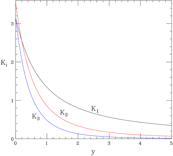
Figure 3: Plot of the functions $K_{1}(y)$, $K_{2}(y)$ and $K_{3}(y)$.

The functions $K_{1},K_{2},K_{3}$ have the following expansions: for small $y$

$$K_{1}(y) = \pi\left[1-\frac{2y}{\sqrt{\pi}}+y^{2}+O(y^{3})\right],$$

$$K_{2}(y) = 2\sqrt{\pi}\left[1-\sqrt{\pi}y+2y^{2}+O(y^{3})\right],$$

$$K_{3}(y) = \pi\left[1-\frac{4y}{\sqrt{\pi}}+3y^{2}+O(y^{3})\right],$$ (133)

while for large $y$

$$K_{1}(y) = \frac{\sqrt{\pi}}{y}\left[1-\frac{1}{2y^{2}}+\frac{3}{4y^{4}}+O\left(\frac{1}{y^{6}}\right)\right],$$

$$K_{2}(y) = \frac{\sqrt{\pi}}{y^{2}}\left[1-\frac{3}{2y^{2}}+O\left(\frac{1}{y^{4}}\right)\right],$$

$$K_{3}(y) = \frac{\sqrt{\pi}}{y^{3}}\left[1+\frac{3}{4y^{2}}+O\left(\frac{1}{y^{4}}\right)\right].$$ (134)

A plot of the functions $K_{1}$, $K_{2}$ and $K_{3}$ is shown in figure 3.

References

- [1] D0 collaboration, Inclusive and b quark production cross-sections in collisions at TeV, Phys. Rev. Lett. 74 (1995) 3548.
- [2] DO collaboration, The production cross-section and angular correlations in collisions at TeV Phys. Lett. B 487 (2000) 264 [hep-ex/9905024].
-
[3]
CDF collaboration, Measurement of the
bottom quark production cross-section using semileptonic decay
electrons in collisions at TeV,
Phys. Rev. Lett. 71 (1993) 500;
Measurement of bottom
quark production in 1.8 TeV collisions using semileptonic
decay muons, Phys. Rev. Lett. 71 (1993) 2396;
Inclusive and b-quark production in collisions at TeV, Phys. Rev. Lett. 71 (1993) 2537;
Measurement of the B meson differential cross-section, , in collisions at TeV, Phys. Rev. Lett. 75 (1995) 1451 [hep-ex/9503013]. - [4] D0 collaboration, Small angle muon and bottom quark production in collisions at TeV, Phys. Rev. Lett. 84 (2000) 5478 [hep-ex/9907029].
- [5] P. Nason, S. Dawson and R.K. Ellis, The total cross-section for the production of heavy quarks in hadronic collisions, Nucl. Phys. B 303 (1988) 607.
- [6] M.L. Mangano, P. Nason and G. Ridolfi, Heavy quark correlations in hadron collisions at next-to-leading order, Nucl. Phys. B 373 (1992) 295.
- [7] W. Beenakker, W.L. van Neerven, R. Meng, G.A. Schuler and J. Smith, QCD corrections to heavy quark production in hadron-hadron collisions, Nucl. Phys. B 351 (1991) 507.
- [8] H1 collaboration, Measurement of open beauty production at HERA, Phys. Lett. B 467 (1999) 156 [hep-ex/9909029].
- [9] ZEUS collaboration, Measurement of open beauty production in photoproduction at HERA, Eur. Phys. J. C 18 (2001) 625 [hep-ex/0011081].
- [10] L3 collaboration, Measurements of the cross sections for open charm and beauty production in collisions at GeV – GeV, Phys. Lett. B 503 (2001) 10 [hep-ex/0011070].
- [11] OPAL collaboration, Charm and bottom production in two-photon collisions with OPAL, hep-ex/0010060.
- [12] S. Frixione and M.L. Mangano, Heavy-quark jets in hadronic collisions, Nucl. Phys. B 483 (1997) 321 [hep-ph/9605270].
- [13] D0 collaboration, Cross section for B jet production in collisions at TeV, Phys. Rev. Lett. 85 (2000) 5068 [hep-ex/0008021].
- [14] R. Bonciani, S. Catani, M.L. Mangano and P. Nason, NLL resummation of the heavy-quark hadroproduction cross-section, Nucl. Phys. B 529 (1998) 424 [hep-ph/9801375].
- [15] R.K. Ellis and D.A. Ross, The coupling of the QCD pomeron in various semihard processes, Nucl. Phys. B 345 (1990) 79.
- [16] S. Catani, M. Ciafaloni and F. Hautmann, Gluon contributions to small x heavy flavor production, Phys. Lett. B 242 (1990) 97.
- [17] J.C. Collins and R.K. Ellis, Heavy quark production in very high-energy hadron collisions, Nucl. Phys. B 360 (1991) 3.
- [18] S. Catani, M. Ciafaloni and F. Hautmann, High-energy factorization and small x heavy flavor production, Nucl. Phys. B 366 (1991) 135.
- [19] S. Catani, M. Ciafaloni and F. Hautmann, Production of heavy flavors at high-energies, CERN-TH-6398-92, presented at the Workshop on Physics at HERA, Hamburg, Germany, Oct 29-30, 1991.
- [20] G. Camici and M. Ciafaloni, Non-abelian contributions to small-x anomalous dimensions, Phys. Lett. B 386 (1996) 341 [hep-ph/9606427].
- [21] G. Camici and M. Ciafaloni, k-factorization and small-x anomalous dimensions, Nucl. Phys. B 496 (1997) 305 [hep-ph/9701303].
- [22] P. Hagler, R. Kirschner, A. Schafer, L. Szymanowski and O. Teryaev, Heavy quark hadroproduction as a test of the effective BFKL vertex, Phys. Rev. D 62 (2000) 071502 [hep-ph/0002077].
- [23] M.G. Ryskin, Y.M. Shabelski and A.G. Shuvaev, Heavy quark production in hadron collisions, hep-ph/0011111.
-
[24]
R.D. Ball and S. Forte, Double asymptotic scaling at HERA,
Phys. Lett. B 335 (1994) 77 [hep-ph/9405320];
A direct test of perturbative QCD at small x, Phys. Lett. B 336 (1994) 77 [hep-ph/9406385]. - [25] R.D. Ball and S. Forte, Summation of leading logarithms at small x, Phys. Lett. B 351 (1995) 313 [hep-ph/9501231].
- [26] R.K. Ellis, F. Hautmann and B.R. Webber, QCD scaling violation at small x, Phys. Lett. B 348 (1995) 582 [hep-ph/9501307].
- [27] S. Forte and R.D. Ball, Double scaling violations, hep-ph/9607291.
-
[28]
I. Bojak and M. Ernst, Small x resummations confronted with
data, Phys. Lett. B 397 (1997) 296 [hep-ph/9609378];
Limitations of small x resummation methods from data, Nucl. Phys. B 508 (1997) 731 [hep-ph/9702282]. - [29] J. Blumlein and A. Vogt, The evolution of unpolarized singlet structure functions at small x, Phys. Rev. D 58 (1998) 014020 [hep-ph/9712546].
- [30] V.S. Fadin and L.N. Lipatov, Bfkl pomeron in the next-to-leading approximation, Phys. Lett. B 429 (1998) 127 [hep-ph/9802290].
- [31] D.A. Ross, The effect of higher order corrections to the BFKL equation on the perturbative pomeron, Phys. Lett. B 431 (1998) 161 [hep-ph/9804332].
- [32] R.D. Ball and S. Forte, Corrections at small x, hep-ph/9805315.
- [33] Y.V. Kovchegov and A.H. Mueller, Running coupling effects in BFKL evolution, Phys. Lett. B 439 (1998) 428 [hep-ph/9805208].
- [34] N. Armesto, J. Bartels and M.A. Braun, On the 2nd order corrections to the hard pomeron and the running coupling, Phys. Lett. B 442 (1998) 459 [hep-ph/9808340].
- [35] G.P. Salam, A resummation of large sub-leading corrections at small x, J. High Energy Phys. 07 (1998) 019 [hep-ph/9806482].
- [36] R.D. Ball and S. Forte, The small x behaviour of Altarelli-Parisi splitting functions, Phys. Lett. B 465 (1999) 271 [hep-ph/9906222].
- [37] M. Ciafaloni, D. Colferai and G.P. Salam, Renormalization group improved small-x equation, Phys. Rev. D 60 (1999) 114036 [hep-ph/9905566].
- [38] G. Altarelli, R.D. Ball and S. Forte, Resummation of singlet parton evolution at small x, Nucl. Phys. B 575 (2000) 313 [hep-ph/9911273].
- [39] G. Altarelli, R.D. Ball and S. Forte, Small-x resummation and hera structure function data, Nucl. Phys. B 599 (2001) 383 [hep-ph/0011270].
- [40] R.K. Ellis and P. Nason, QCD radiative corrections to the photoproduction of heavy quarks, Nucl. Phys. B 312 (1989) 551.
- [41] S. Catani, Comment on quarks and gluons at small x and the SDIS factorization scheme, Z. Physik C 70 (1996) 263 [hep-ph/9506357]; Quarks and gluons at small x and scaling violation of , hep-ph/9506348.
- [42] R.D. Ball and S. Forte, Momentum conservation at small x, Phys. Lett. B 359 (1995) 362 [hep-ph/9507321].
- [43] S. Catani and F. Hautmann, High-energy factorization and small x deep inelastic scattering beyond leading order, Nucl. Phys. B 427 (1994) 475 [hep-ph/9405388].
- [44] A.D. Rujula, S.L. Glashow, H.D. Politzer, S.B. Treiman, F. Wilczek and A. Zee, Possible nonregge behavior of electroproduction structure functions, Phys. Rev. D 10 (1974) 1649.