Study of relativistic bound states in a scalar model using diagonalization/Monte Carlo methods

Buḡra Borasoya and Dean Leeb
aPhysik Department, Technische Universität München, D-85747 Garching, Germany
bDept. of Physics, Univ. of Massachusetts, Amherst, MA 01003, U.S.A.

borasoy@physik.tu-muenchen.dedlee@physics.umass.edu
Abstract

We use a recently proposed diagonalization/Monte Carlo computational scheme to study relativistic two-body and three-body bound states in (ϕ6ϕ4)1+1subscriptsuperscriptitalic-ϕ6superscriptitalic-ϕ411(\phi^{6}-\phi^{4})_{1+1} theory.  We find that the approach is well-suited for calculating bound state energies and wavefunctions.

1 Introduction

The structure and phenomenology of relativistic bound states are of primary interest to particle and nuclear physics.  Unfortunately even in the simplest field theory models our understanding of relativistic bound states is limited by a number of complications.  Monte Carlo simulation on the lattice is the standard tool for determining particle masses.  One can find the low energy spectrum from the decay constants of Euclidean correlation functions.  Though the procedure is generally successful it becomes more difficult and less reliable if the state of interest has the same quantum numbers as another lower energy state.  Complications also arise for non-confining interactions, where states just above the continuum threshold can obscure the signal of the bound state.  Both of these problems arise even in seemingly simple systems such as we consider here, namely, two-body and three-body bound states in (ϕ6ϕ4)1+1subscriptsuperscriptitalic-ϕ6superscriptitalic-ϕ411(\phi^{6}-\phi^{4})_{1+1}.

One remaining complication is of a more operational nature, and it concerns the interface between computational methods and phenomenology.  Much of the interesting and important physics associated with bound states is contained in subtle details.  A measurement of gross properties such as the binding energy is a necessary first step, but one also hopes to gain more descriptive information like the structure of the wavefunction, its response to various interactions, or point-by-point comparisons with intuitive non-relativistic models.

These issues were part of the motivation for a recently proposed approach to computational quantum problems which combines diagonalization and Monte Carlo techniques [1, 2].  Diagonalization makes it possible to consider systems with sign oscillations and extract detailed information about wavefunctions and excited states, while Monte Carlo allows one to handle the exponential increase in the number of basis states for large volume systems.  The first half of the method involves finding and diagonalizing the Hamiltonian restricted to an optimal subspace.  This subspace is designed to include the most important basis vectors of the lowest energy eigenstates.  Once the most important basis vectors are found and their interactions treated exactly, Monte Carlo is used to sample the contribution of the remaining basis vectors.  In this paper we demonstrate how the new diagonalization/Monte Carlo scheme is applied to the study of relativistic bound states.

The essential problem of the lattice Monte Carlo approach to bound states near the continuum threshold involves finding the inverse Laplace transform of two-point correlation functions at energies close to thresholds where the spectral density is large. This is usually done by a non-linear multi-parameter fit of two-point correlators for several different operators. While in principle one might reach arbitrary accuracy by adding more parameters to the fit, in practice the presence of even very small stochastic error will destabilize the fit and imposes an upper limit on the accuracy. The main advantage of our method, therefore, is not in computing speed but in numerical stability. Our method also provides additional information about the wavefunction of the bound state. These two statements are not unrelated. Our method has greater numerical stability because we are implicitly using the information contained in the wavefunctions to separate states. It is also worthwhile noting that in two dimensions the diagonalization/Monte Carlo approach can be applied within the framework of discretized light cone and might prove useful since, aside from zero-mode problems, the exponential growth of the number of basis states for large volume systems has so far provided a limit to discretized light cone.

The organization of the paper is as follows.  We begin with a discussion of the ϕ6ϕ4superscriptitalic-ϕ6superscriptitalic-ϕ4\phi^{6}-\phi^{4} Hamiltonian in 1+1111+1 dimensions and its decomposition into momentum modes.  We then review the basic features of quasi-sparse eigenvector diagonalization and stochastic error correction.  In the following two sections we briefly set aside the numerical discussion and derive solutions to the non-relativistic versions of the two-body and three-body bound state problems.  We then compare our numerical results for the relativistic bound states energies and wavefunctions with an assortment of different approximations and results from the literature.

2 Fock states and the Hamiltonian

Our starting point is the Hamiltonian density for ϕ6ϕ4superscriptitalic-ϕ6superscriptitalic-ϕ4\phi^{6}-\phi^{4} theory in 1+1111+1 dimensions,

=:12(ϕt)2+12(ϕx)2+μ22ϕ2+λ(ϕ6ϕ4):,:12superscriptitalic-ϕ𝑡212superscriptitalic-ϕ𝑥2superscript𝜇22superscriptitalic-ϕ2𝜆superscriptitalic-ϕ6superscriptitalic-ϕ4:,\mathcal{H}=\text{:}\tfrac{1}{2}\left(\tfrac{\partial\phi}{\partial t}\right)^{2}+\tfrac{1}{2}\left(\tfrac{\partial\phi}{\partial x}\right)^{2}+\tfrac{\mu^{2}}{2}\phi^{2}+\lambda\left(\phi^{6}-\phi^{4}\right)\text{:,} (1)

where normal ordering is with respect to the mass μ𝜇\mu.  This theory was introduced in [3] as a simple model with a stable bound state.  In 1+1111+1 dimensions, normal ordering is sufficient to renormalize the theory.

We will consider the theory in a periodic box of length 2L2𝐿2L.  This allows us to expand in free particle momentum modes and rewrite the Hamiltonian in terms of mode creation and annihilation operators [1, 5],

H𝐻\displaystyle H =nωn(μ)ananλ8Ln1++n4=0:(an1+an1)ωn1(μ)(an4+an4)ωn4(μ)::absentsubscript𝑛subscript𝜔𝑛𝜇superscriptsubscript𝑎𝑛subscript𝑎𝑛𝜆8𝐿subscriptsubscript𝑛1subscript𝑛40subscript𝑎subscript𝑛1superscriptsubscript𝑎subscript𝑛1subscript𝜔subscript𝑛1𝜇subscript𝑎subscript𝑛4superscriptsubscript𝑎subscript𝑛4subscript𝜔subscript𝑛4𝜇:absent\displaystyle={\displaystyle\sum_{n}}\omega_{n}(\mu)a_{n}^{\dagger}a_{n}-\tfrac{\lambda}{8L}{\displaystyle\sum_{n_{1}+\cdots+n_{4}=0}}:\tfrac{\left(a_{n_{1}}+a_{-n_{1}}^{\dagger}\right)}{\sqrt{\omega_{n_{1}}(\mu)}}\cdots\tfrac{\left(a_{n_{4}}+a_{-n_{4}}^{\dagger}\right)}{\sqrt{\omega_{n_{4}}(\mu)}}: (2)
+λ32L2n1++n6=0:(an1+an1)ωn1(μ)(an6+an6)ωn6(μ):.:𝜆32superscript𝐿2subscriptsubscript𝑛1subscript𝑛60subscript𝑎subscript𝑛1superscriptsubscript𝑎subscript𝑛1subscript𝜔subscript𝑛1𝜇subscript𝑎subscript𝑛6superscriptsubscript𝑎subscript𝑛6subscript𝜔subscript𝑛6𝜇:absent\displaystyle+\tfrac{\lambda}{32L^{2}}{\displaystyle\sum_{n_{1}+\cdots+n_{6}=0}}:\tfrac{\left(a_{n_{1}}+a_{-n_{1}}^{\dagger}\right)}{\sqrt{\omega_{n_{1}}(\mu)}}\cdots\tfrac{\left(a_{n_{6}}+a_{-n_{6}}^{\dagger}\right)}{\sqrt{\omega_{n_{6}}(\mu)}}:.

In (2) we have used

ωn(μ)=n2π2L2+μ2.subscript𝜔𝑛𝜇superscript𝑛2superscript𝜋2superscript𝐿2superscript𝜇2\omega_{n}(\mu)=\sqrt{\tfrac{n^{2}\pi^{2}}{L^{2}}+\mu^{2}}. (3)

We can represent any momentum-space Fock state as a string of occupation numbers, |oNmax,,oNmaxketsubscript𝑜subscript𝑁subscript𝑜subscript𝑁\left|o_{-N_{\max}},\cdots,o_{N_{\max}}\right\rangle, where

anan|oNmax,,oNmax=on|oNmax,,oNmax.superscriptsubscript𝑎𝑛subscript𝑎𝑛ketsubscript𝑜subscript𝑁subscript𝑜subscript𝑁subscript𝑜𝑛ketsubscript𝑜subscript𝑁subscript𝑜subscript𝑁a_{n}^{\dagger}a_{n}\left|o_{-N_{\max}},\cdots,o_{N_{\max}}\right\rangle=o_{n}\left|o_{-N_{\max}},\cdots,o_{N_{\max}}\right\rangle. (4)

For the calculations presented here, we set the length of the box to size L=2.5πμ1𝐿2.5𝜋superscript𝜇1L=2.5\pi\mu^{-1} and restrict our attention to momentum modes such that |n|Nmax𝑛subscript𝑁\left|n\right|\leq N_{\max}, where Nmax=10subscript𝑁10N_{\max}=10.  This corresponds with a momentum cutoff scale of Λ=4μ.Λ4𝜇\Lambda=4\mu. A change in the cutoff Nmaxsubscript𝑁N_{\max} will lead to adjustments in μ𝜇\mu and λ𝜆\lambda in order to keep the physics independent of Nmaxsubscript𝑁N_{\max}. However, these corrections begin at 𝒪(1/Nmax2)𝒪1superscriptsubscript𝑁2{\cal O}(1/N_{\max}^{2}) as can be checked by power counting. The dependence on Nmaxsubscript𝑁N_{\max} has been measured explicitly for the bound state data presented in this paper. It is considerably smaller than the dominant error, which is due to higher order corrections in the series stochastic error method, see below.

3 QSE diagonalization

In order to find approximate eigenvalues and eigenvectors of the Hamiltonian in (2), we use a method called quasi-sparse eigenvector (QSE) diagonalization.  QSE diagonalization is an iterative algorithm that finds the most important basis vectors of the low energy eigenstates for a quantum Hamiltonian.  We follow closely the discussion presented in [1].  We start with a complete basis for which the Hamiltonian matrix Hijsubscript𝐻𝑖𝑗H_{ij} is sparse.  In our case we use the momentum-space Fock basis.  The QSE method involves the following iterated steps:

  1. 1.

    Select a subset of basis vectors {ei1,,ein}subscript𝑒subscript𝑖1subscript𝑒subscript𝑖𝑛\left\{e_{i_{1}},\cdots,e_{i_{n}}\right\} and call the corresponding subspace S𝑆S.

  2. 2.

    Diagonalize H𝐻H restricted to S𝑆S and find one eigenvector v𝑣v.

  3. 3.

    Sort the basis components of v𝑣v according to their magnitude and remove the least important basis vectors.

  4. 4.

    Replace the discarded basis vectors by new basis vectors.  These are selected at random from a pool of candidate basis vectors which are connected to the old basis vectors through non-vanishing matrix elements of H𝐻H.

  5. 5.

    Redefine S𝑆S as the subspace spanned by the updated set of basis vectors and repeat steps 2 through 5.

If the subset of basis vectors is sufficiently large, the exact low energy eigenvectors will be stable fixed points of the update process.  This is the single eigenvector version of the algorithm.  The multiple eigenvector version simply involves selecting more than one eigenvector each iteration and retaining the most important basis vectors for each of the eigenvectors. One of the most attractive features of our method is that we are working directly with the infinite dimensional Hilbert space. There is no restriction on the maximum occupation for any mode. This is a clear advantage over standard diagonalization methods such as Lanczos.

In this analysis we work in the rest frame of the bound state and consider Fock states with total momentum zero.  Due to ϕϕitalic-ϕitalic-ϕ\phi\rightarrow-\phi reflection symmetry we can diagonalize the even and odd ϕitalic-ϕ\phi sectors separately.  We use the multiple eigenvector algorithm to obtain the four lowest eigenstates in the even sector and in the odd sector.111We have found only one two-body bound state and one three-body bound state.  Thus in a follow-up study one could suffice with fewer states in each sector.  For each QSE iteration, we select 505050 new basis vectors and keep 400400400 basis vectors.  The final QSE results are used as the starting point for the stochastic error correction method.

4 Stochastic error correction

The QSE method approximates the low energy eigenvalues and eigenvectors of the Hamiltonian by finding and diagonalizing optimized subspaces S𝑆S.  This process however has an intrinsic error due to the omission of basis states not in S𝑆S.  The goal of stochastic error correction is to sample the contribution of these remaining basis vectors.  In the present investigation we use the so-called series expansion method up to first order.  This has been explained in detail in [2, 4] and therefore we restrict ourselves to the review of basic formulae.

Let λisubscript𝜆𝑖\lambda_{i} be an eigenvalue and |viketsubscript𝑣𝑖|v_{i}\rangle be the corresponding eigenvector of H𝐻H restricted to the subspace S𝑆S (the span of the subset of basis vectors after step 3 of the QSE algorithm).  The remaining basis vectors in the full space not contained in S𝑆S will be denoted by |Aiketsubscript𝐴𝑖|A_{i}\rangle, and we are interested in sampling the contribution of these vectors.  We assume that λ1subscript𝜆1\lambda_{1} and |v1ketsubscript𝑣1|v_{1}\rangle are close to the corresponding quantities for the full Hamiltonian H𝐻H.  If we now expand in powers of

(Ai|H|Aiλ1)1superscriptquantum-operator-productsubscript𝐴𝑖𝐻subscript𝐴𝑖subscript𝜆11\left(\langle A_{i}|H|A_{i}\rangle-\lambda_{1}\right)^{-1} (5)

we find that the first order correction to λ1subscript𝜆1\lambda_{1} is

δλ1=iv1|H|AiAi|H|v1Ai|H|Aiλ1𝛿subscript𝜆1subscript𝑖quantum-operator-productsubscript𝑣1𝐻subscript𝐴𝑖quantum-operator-productsubscript𝐴𝑖𝐻subscript𝑣1quantum-operator-productsubscript𝐴𝑖𝐻subscript𝐴𝑖subscript𝜆1\delta\lambda_{1}=-\sum_{i}\tfrac{\langle v_{1}|H|A_{i}\rangle\langle A_{i}|H|v_{1}\rangle}{\langle A_{i}|H|A_{i}\rangle-\lambda_{1}} (6)

and the first order correction to |v1ketsubscript𝑣1|v_{1}\rangle is

|δv1=i|AiAi|H|v1Ai|H|Aiλ1+j1i|vjvj|H|AiAi|H|v1(λjλ1)(Ai|H|Aiλ1).ket𝛿subscript𝑣1subscript𝑖ketsubscript𝐴𝑖quantum-operator-productsubscript𝐴𝑖𝐻subscript𝑣1quantum-operator-productsubscript𝐴𝑖𝐻subscript𝐴𝑖subscript𝜆1subscript𝑗1subscript𝑖ketsubscript𝑣𝑗quantum-operator-productsubscript𝑣𝑗𝐻subscript𝐴𝑖quantum-operator-productsubscript𝐴𝑖𝐻subscript𝑣1subscript𝜆𝑗subscript𝜆1quantum-operator-productsubscript𝐴𝑖𝐻subscript𝐴𝑖subscript𝜆1\left|\delta v_{1}\right\rangle=-\sum_{i}\tfrac{\left|A_{i}\right\rangle\langle A_{i}|H|v_{1}\rangle}{\langle A_{i}|H|A_{i}\rangle-\lambda_{1}}+\sum_{j\neq 1}\sum_{i}\tfrac{\left|v_{j}\right\rangle\langle v_{j}|H|A_{i}\rangle\langle A_{i}|H|v_{1}\rangle}{(\lambda_{j}-\lambda_{1})(\langle A_{i}|H|A_{i}\rangle-\lambda_{1})}. (7)

The sum over all vectors |Aiketsubscript𝐴𝑖|A_{i}\rangle is too unwieldy to perform exactly.  Instead we sample the sum stochastically in the following manner.  Let P(Atrial(i))𝑃subscript𝐴trial𝑖P(A_{\text{trial}(i)}) be the probability of selecting |Atrial(i)ketsubscript𝐴trial𝑖\left|A_{\text{trial}(i)}\right\rangle on the ithsuperscript𝑖thi^{\text{th}} trial.  Then

δλ1=limN1Ni=1,,Nv1|H|Atrial(i)Atrial(i)|H|v1(Atrial(i)|H|Atrial(i)λ1)P(Atrial(i))𝛿subscript𝜆1subscript𝑁1𝑁subscript𝑖1𝑁quantum-operator-productsubscript𝑣1𝐻subscript𝐴trial𝑖quantum-operator-productsubscript𝐴trial𝑖𝐻subscript𝑣1quantum-operator-productsubscript𝐴trial𝑖𝐻subscript𝐴trial𝑖subscript𝜆1𝑃subscript𝐴trial𝑖\delta\lambda_{1}=-\lim_{N\rightarrow\infty}\frac{1}{N}\sum_{i=1,...,N}\tfrac{\langle v_{1}|H|A_{\text{trial}(i)}\rangle\langle A_{\text{trial}(i)}|H|v_{1}\rangle}{(\langle A_{\text{trial}(i)}|H|A_{\text{trial}(i)}\rangle-\lambda_{1})P(A_{\text{trial}(i)})} (8)

and

w|δv1inner-product𝑤𝛿subscript𝑣1\displaystyle\left\langle w\right.\left|\delta v_{1}\right\rangle =limN1Niw|Atrial(i)Atrial(i)|H|v1(Atrial(i)|H|Atrial(i)λ1)P(Atrial(i))absentsubscript𝑁1𝑁subscript𝑖inner-product𝑤subscript𝐴trial𝑖quantum-operator-productsubscript𝐴trial𝑖𝐻subscript𝑣1quantum-operator-productsubscript𝐴trial𝑖𝐻subscript𝐴trial𝑖subscript𝜆1𝑃subscript𝐴trial𝑖\displaystyle=-\lim_{N\rightarrow\infty}\frac{1}{N}\sum_{i}\tfrac{\left\langle w\right.\left|A_{\text{trial}(i)}\right\rangle\langle A_{\text{trial}(i)}|H|v_{1}\rangle}{(\langle A_{\text{trial}(i)}|H|A_{\text{trial}(i)}\rangle-\lambda_{1})P(A_{\text{trial}(i)})} (9)
+limN1Nj1iw|vjvj|H|Atrial(i)Atrial(i)|H|v1(λjλ1)(Atrial(i)|H|Atrial(i)λ1)P(Atrial(i))subscript𝑁1𝑁subscript𝑗1subscript𝑖inner-product𝑤subscript𝑣𝑗quantum-operator-productsubscript𝑣𝑗𝐻subscript𝐴trial𝑖quantum-operator-productsubscript𝐴trial𝑖𝐻subscript𝑣1subscript𝜆𝑗subscript𝜆1quantum-operator-productsubscript𝐴trial𝑖𝐻subscript𝐴trial𝑖subscript𝜆1𝑃subscript𝐴trial𝑖\displaystyle+\lim_{N\rightarrow\infty}\frac{1}{N}\sum_{j\neq 1}\sum_{i}\tfrac{\left\langle w\right.\left|v_{j}\right\rangle\langle v_{j}|H|A_{\text{trial}(i)}\rangle\langle A_{\text{trial}(i)}|H|v_{1}\rangle}{(\lambda_{j}-\lambda_{1})(\langle A_{\text{trial}(i)}|H|A_{\text{trial}(i)}\rangle-\lambda_{1})P(A_{\text{trial}(i)})}

for any fixed vector |wket𝑤\left|w\right\rangle.

5 Two-body bound state

Before presenting the results of our calculations, we first summarize what we expect in the weak-coupling non-relativistic limit.  For the two-body bound state we consider all two-particle Fock states with zero momentum,

|n,n=anan|0.ket𝑛𝑛superscriptsubscript𝑎𝑛superscriptsubscript𝑎𝑛ket0\left|n,-n\right\rangle=a_{n}^{\dagger}a_{-n}^{\dagger}\left|0\right\rangle. (10)

These states satisfy the orthogonality and normalization conditions

n,n|n,n=δn,n+δn,n.inner-productsuperscript𝑛superscript𝑛𝑛𝑛subscript𝛿𝑛superscript𝑛subscript𝛿𝑛superscript𝑛\left\langle n^{\prime},-n^{\prime}\right|\left.n,-n\right\rangle=\delta_{n,n^{\prime}}+\delta_{n,-n^{\prime}}. (11)

At lowest order in λ𝜆\lambda the :ϕ6::\phi^{6}: interaction is not relevant to the two-body bound state problem.  The effective interaction Hamiltonian is therefore

HIsubscript𝐻𝐼\displaystyle H_{I} =λ:ϕ4::absent𝜆superscriptitalic-ϕ4:absent\displaystyle=-\lambda:\phi^{4}: (12)
=3λ4Ln1+n2+n3+n4=0an1an2an3an4(μ2+n12π2L2)1/4(μ2+n22π2L2)1/4(μ2+n32π2L2)1/4(μ2+n42π2L2)1/4.absent3𝜆4𝐿subscriptsubscript𝑛1subscript𝑛2subscript𝑛3subscript𝑛40superscriptsubscript𝑎subscript𝑛1superscriptsubscript𝑎subscript𝑛2subscript𝑎subscript𝑛3subscript𝑎subscript𝑛4superscriptsuperscript𝜇2superscriptsubscript𝑛12superscript𝜋2superscript𝐿214superscriptsuperscript𝜇2superscriptsubscript𝑛22superscript𝜋2superscript𝐿214superscriptsuperscript𝜇2superscriptsubscript𝑛32superscript𝜋2superscript𝐿214superscriptsuperscript𝜇2superscriptsubscript𝑛42superscript𝜋2superscript𝐿214\displaystyle=-\tfrac{3\lambda}{4L}\sum_{n_{1}+n_{2}+n_{3}+n_{4}=0}\tfrac{a_{-n_{1}}^{\dagger}a_{-n_{2}}^{\dagger}a_{n_{3}}a_{n_{4}}}{\left(\mu^{2}+\frac{n_{1}^{2}\pi^{2}}{L^{2}}\right)^{1/4}\left(\mu^{2}+\frac{n_{2}^{2}\pi^{2}}{L^{2}}\right)^{1/4}\left(\mu^{2}+\frac{n_{3}^{2}\pi^{2}}{L^{2}}\right)^{1/4}\left(\mu^{2}+\frac{n_{4}^{2}\pi^{2}}{L^{2}}\right)^{1/4}}.

In the non-relativistic limit we can approximate HIsubscript𝐻𝐼H_{I} as

HI=3λ4μ2Ln1+n2+n3+n4=0an1an2an3an4.subscript𝐻𝐼3𝜆4superscript𝜇2𝐿subscriptsubscript𝑛1subscript𝑛2subscript𝑛3subscript𝑛40superscriptsubscript𝑎subscript𝑛1superscriptsubscript𝑎subscript𝑛2subscript𝑎subscript𝑛3subscript𝑎subscript𝑛4H_{I}=-\tfrac{3\lambda}{4\mu^{2}L}\sum_{n_{1}+n_{2}+n_{3}+n_{4}=0}a_{-n_{1}}^{\dagger}a_{-n_{2}}^{\dagger}a_{n_{3}}a_{n_{4}}. (13)

It is convenient to define the position-space basis vectors

|x=12Ln=0,±1,einπxL|n,n.ket𝑥12𝐿subscript𝑛0plus-or-minus1superscript𝑒𝑖𝑛𝜋𝑥𝐿ket𝑛𝑛\left|x\right\rangle=\tfrac{1}{\sqrt{2L}}\sum_{n=0,\pm 1,...}e^{i\frac{n\pi x}{L}}\left|n,-n\right\rangle. (14)

Since we are considering a periodic box,

|x=|x+2Lket𝑥ket𝑥2𝐿\left|x\right\rangle=\left|x+2L\right\rangle (15)

and the position-space vectors satisfy

x|x=j=0,±1,[δ(xx+2jL)+δ(x+x+2jL)].inner-productsuperscript𝑥𝑥subscript𝑗0plus-or-minus1delimited-[]𝛿superscript𝑥𝑥2𝑗𝐿𝛿superscript𝑥𝑥2𝑗𝐿\left\langle x^{\prime}\right|\left.x\right\rangle={\displaystyle\sum_{j=0,\pm 1,...}}\left[\delta(x^{\prime}-x+2jL)+\delta(x^{\prime}+x+2jL)\right]. (16)

For any function Ψ(x)Ψ𝑥\Psi(x), we can define

|Ψ=LL𝑑xΨ(x)|x.ketΨsuperscriptsubscript𝐿𝐿differential-d𝑥Ψ𝑥ket𝑥\left|\Psi\right\rangle=\int_{-L}^{L}dx\Psi(x)\left|x\right\rangle. (17)

If |ΨketΨ\left|\Psi\right\rangle is to have unit norm, then we require

LL𝑑x|Ψ(x)|2=12.superscriptsubscript𝐿𝐿differential-d𝑥superscriptΨ𝑥212\int_{-L}^{L}dx\left|\Psi(x)\right|^{2}=\tfrac{1}{2}. (18)

In our position-space representation of the two-particle subspace, we note that

n=0,±1,anan|x=2|xsubscript𝑛0plus-or-minus1superscriptsubscript𝑎𝑛subscript𝑎𝑛ket𝑥2ket𝑥\sum_{n=0,\pm 1,...}a_{n}^{\dagger}a_{n}\left|x\right\rangle=2\left|x\right\rangle (19)

and

n=0,±1,n2π2L2anan|Ψ=2|2Ψx2.subscript𝑛0plus-or-minus1superscript𝑛2superscript𝜋2superscript𝐿2superscriptsubscript𝑎𝑛subscript𝑎𝑛ketΨ2ketsuperscript2Ψsuperscript𝑥2\sum_{n=0,\pm 1,...}\tfrac{n^{2}\pi^{2}}{L^{2}}a_{n}^{\dagger}a_{n}\left|\Psi\right\rangle=-2\left|\tfrac{\partial^{2}\Psi}{\partial x^{2}}\right\rangle. (20)

Upon restricting our Hilbert space to the zero-momentum two-particle subspace, we can simplify the interaction Hamiltonian by the substitution

n1+n2+n3+n4=0an1an2an3an4n1,n2an1an1an2an2.subscriptsubscript𝑛1subscript𝑛2subscript𝑛3subscript𝑛40superscriptsubscript𝑎subscript𝑛1superscriptsubscript𝑎subscript𝑛2subscript𝑎subscript𝑛3subscript𝑎subscript𝑛4subscriptsubscript𝑛1subscript𝑛2superscriptsubscript𝑎subscript𝑛1superscriptsubscript𝑎subscript𝑛1subscript𝑎subscript𝑛2subscript𝑎subscript𝑛2\sum_{n_{1}+n_{2}+n_{3}+n_{4}=0}a_{-n_{1}}^{\dagger}a_{-n_{2}}^{\dagger}a_{n_{3}}a_{n_{4}}\rightarrow\sum_{n_{1},n_{2}}a_{n_{1}}^{\dagger}a_{-n_{1}}^{\dagger}a_{n_{2}}a_{-n_{2}}. (21)

We observe that

n1,n2an1an1an2an2|x=4Lδ(x)|x.subscriptsubscript𝑛1subscript𝑛2superscriptsubscript𝑎subscript𝑛1superscriptsubscript𝑎subscript𝑛1subscript𝑎subscript𝑛2subscript𝑎subscript𝑛2ket𝑥4𝐿𝛿𝑥ket𝑥\sum_{n_{1},n_{2}}a_{n_{1}}^{\dagger}a_{-n_{1}}^{\dagger}a_{n_{2}}a_{-n_{2}}\left|x\right\rangle=4L\delta(x)\left|x\right\rangle. (22)

The full non-relativistic Hamiltonian,

H=n=0,±1,(μ+n2π22μL2)anan3λ4μ2Ln1,n2an1an1an2an2,𝐻subscript𝑛0plus-or-minus1𝜇superscript𝑛2superscript𝜋22𝜇superscript𝐿2superscriptsubscript𝑎𝑛subscript𝑎𝑛3𝜆4superscript𝜇2𝐿subscriptsubscript𝑛1subscript𝑛2superscriptsubscript𝑎subscript𝑛1superscriptsubscript𝑎subscript𝑛1subscript𝑎subscript𝑛2subscript𝑎subscript𝑛2H=\sum_{n=0,\pm 1,...}\left(\mu+\tfrac{n^{2}\pi^{2}}{2\mu L^{2}}\right)a_{n}^{\dagger}a_{n}-\tfrac{3\lambda}{4\mu^{2}L}\sum_{n_{1},n_{2}}a_{n_{1}}^{\dagger}a_{-n_{1}}^{\dagger}a_{n_{2}}a_{-n_{2}}, (23)

can now be represented as a Schrödinger operator:

(H2μ)Ψ(x)=[1μ2x23λμ2δ(x)]Ψ(x).𝐻2𝜇Ψ𝑥delimited-[]1𝜇superscript2superscript𝑥23𝜆superscript𝜇2𝛿𝑥Ψ𝑥(H-2\mu)\Psi(x)=\left[-\tfrac{1}{\mu}\tfrac{\partial^{2}}{\partial x^{2}}-\tfrac{3\lambda}{\mu^{2}}\delta(x)\right]\Psi(x). (24)

We now consider the eigenvalue equation

(H2μ)Ψ(x)=EΨ(x).𝐻2𝜇Ψ𝑥𝐸Ψ𝑥(H-2\mu)\Psi(x)=E\Psi(x). (25)

Using the ansatz

Ψ2(x)subscriptΨ2𝑥\displaystyle\Psi_{2}(x) eb|x|+ce+b|x|,proportional-toabsentsuperscript𝑒𝑏𝑥𝑐superscript𝑒𝑏𝑥\displaystyle\propto e^{-b\left|x\right|}+ce^{+b\left|x\right|}, (26)
b𝑏\displaystyle b >0,absent0\displaystyle>0, (27)

we find

c𝑐\displaystyle c =e3λLμ1+c1c,absentsuperscript𝑒3𝜆𝐿𝜇1𝑐1𝑐\displaystyle=e^{-\tfrac{3\lambda L}{\mu}\tfrac{1+c}{1-c}}, (28)
b𝑏\displaystyle b =3λ2μ1+c1c,absent3𝜆2𝜇1𝑐1𝑐\displaystyle=\tfrac{3\lambda}{2\mu}\tfrac{1+c}{1-c}, (29)
E𝐸\displaystyle E =b2μ.absentsuperscript𝑏2𝜇\displaystyle=-\tfrac{b^{2}}{\mu}. (30)

When

e3λLμ<<1,much-less-thansuperscript𝑒3𝜆𝐿𝜇1e^{-\tfrac{3\lambda L}{\mu}}<<1, (31)

we have

c𝑐\displaystyle c =e3λLμ(1+O(e3λLμ)),absentsuperscript𝑒3𝜆𝐿𝜇1𝑂superscript𝑒3𝜆𝐿𝜇\displaystyle=e^{-\tfrac{3\lambda L}{\mu}}(1+O(e^{-\tfrac{3\lambda L}{\mu}})), (32)
b𝑏\displaystyle b =3λ2μ(1+O(e3λLμ)),absent3𝜆2𝜇1𝑂superscript𝑒3𝜆𝐿𝜇\displaystyle=\tfrac{3\lambda}{2\mu}(1+O(e^{-\tfrac{3\lambda L}{\mu}})), (33)
E𝐸\displaystyle E =9λ24μ3(1+O(e3λLμ)).absent9superscript𝜆24superscript𝜇31𝑂superscript𝑒3𝜆𝐿𝜇\displaystyle=-\tfrac{9\lambda^{2}}{4\mu^{3}}(1+O(e^{-\tfrac{3\lambda L}{\mu}})). (34)

This expression for the binding energy is consistent with the derivation in [6].  In the infinite L𝐿L limit we obtain

Ψ2(x)=3λ4μe3λ|x|2μ.subscriptΨ2𝑥3𝜆4𝜇superscript𝑒3𝜆𝑥2𝜇\Psi_{2}(x)=\sqrt{\tfrac{3\lambda}{4\mu}}e^{-\tfrac{3\lambda\left|x\right|}{2\mu}}. (35)

6 Three-body bound state

The analysis for the three-body bound state is slightly more involved.  In the non-relativistic weak-coupling limit we restrict our attention to three-particle states with zero-momentum,

|n1,n2,n1n2=an1an2an1n2|0.ketsubscript𝑛1subscript𝑛2subscript𝑛1subscript𝑛2superscriptsubscript𝑎subscript𝑛1superscriptsubscript𝑎subscript𝑛2superscriptsubscript𝑎subscript𝑛1subscript𝑛2ket0\left|n_{1},n_{2},-n_{1}-n_{2}\right\rangle=a_{n_{1}}^{\dagger}a_{n_{2}}^{\dagger}a_{-n_{1}-n_{2}}^{\dagger}\left|0\right\rangle. (36)

We again construct position-space basis states

|x1,x2=32Ln1,n2=0,±1,ein1πx1Lein2πx2Lei(n1n2)π(x1x2)L|n1,n2,n1n2,ketsubscript𝑥1subscript𝑥232𝐿subscriptformulae-sequencesubscript𝑛1subscript𝑛20plus-or-minus1superscript𝑒𝑖subscript𝑛1𝜋subscript𝑥1𝐿superscript𝑒𝑖subscript𝑛2𝜋subscript𝑥2𝐿superscript𝑒𝑖subscript𝑛1subscript𝑛2𝜋subscript𝑥1subscript𝑥2𝐿ketsubscript𝑛1subscript𝑛2subscript𝑛1subscript𝑛2\left|x_{1},x_{2}\right\rangle=\tfrac{\sqrt{3}}{2L}\sum_{n_{1},n_{2}=0,\pm 1,...}e^{i\frac{n_{1}\pi x_{1}}{L}}e^{i\frac{n_{2}\pi x_{2}}{L}}e^{i\frac{(-n_{1}-n_{2})\pi(-x_{1}-x_{2})}{L}}\left|n_{1},n_{2},-n_{1}-n_{2}\right\rangle, (37)

which satisfy the orthogonality and normalization conditions

x1,x2|x1,x2=j,k=0,±1,[δ(x1x1+(2j3+2k)L)δ(x2x2+2j3L)+{x1x2x1x2}].\left\langle x_{1}^{\prime},x_{2}^{\prime}\right|\left.x_{1},x_{2}\right\rangle={\displaystyle\sum_{j,k=0,\pm 1,...}}\left[\begin{array}[c]{c}\delta(x_{1}^{\prime}-x_{1}+(\frac{2j}{3}+2k)L)\delta(x_{2}^{\prime}-x_{2}+\frac{2j}{3}L)\\ +\left\{x_{1}\leftrightarrow x_{2}\leftrightarrow-x_{1}-x_{2}\right\}\end{array}\right]. (38)

The periodicity of our system implies

|x1,x2ketsubscript𝑥1subscript𝑥2\displaystyle\left|x_{1},x_{2}\right\rangle =|x1+23L,x2+23Labsentketsubscript𝑥123𝐿subscript𝑥223𝐿\displaystyle=\left|x_{1}+\tfrac{2}{3}L,x_{2}+\tfrac{2}{3}L\right\rangle (39)
=|x1+2L,x2=|x1,x2+2L.absentketsubscript𝑥12𝐿subscript𝑥2ketsubscript𝑥1subscript𝑥22𝐿\displaystyle=\left|x_{1}+2L,x_{2}\right\rangle=\left|x_{1},x_{2}+2L\right\rangle.

For any function Ψ(x1,x2)Ψsubscript𝑥1subscript𝑥2\Psi(x_{1},x_{2}), we define

|Ψ=R𝑑x1𝑑x2𝑑Ψ(x1,x2)|x1,x2,ketΨsubscript𝑅differential-dsubscript𝑥1differential-dsubscript𝑥2differential-dΨsubscript𝑥1subscript𝑥2ketsubscript𝑥1subscript𝑥2\left|\Psi\right\rangle=\int_{R}dx_{1}dx_{2}d\Psi(x_{1},x_{2})\left|x_{1},x_{2}\right\rangle, (40)

where R𝑅R is the region

R={L<x1L13L<x213L.𝑅cases𝐿subscript𝑥1𝐿13𝐿subscript𝑥213𝐿R=\left\{\begin{array}[c]{c}-L<x_{1}\leq L\\ -\tfrac{1}{3}L<x_{2}\leq\tfrac{1}{3}L.\end{array}\right. (41)

If |ΨketΨ\left|\Psi\right\rangle is to have unit norm then we must have

R𝑑x1𝑑x2|Ψ(x1,x2)|2=16.subscript𝑅differential-dsubscript𝑥1differential-dsubscript𝑥2superscriptΨsubscript𝑥1subscript𝑥2216\int_{R}dx_{1}dx_{2}\left|\Psi(x_{1},x_{2})\right|^{2}=\tfrac{1}{6}. (42)

We note that

n=0,±1,n2π2L2anan|Ψ=23|2Ψx12+2Ψx222Ψx1x2.subscript𝑛0plus-or-minus1superscript𝑛2superscript𝜋2superscript𝐿2superscriptsubscript𝑎𝑛subscript𝑎𝑛ketΨ23ketsuperscript2Ψsuperscriptsubscript𝑥12superscript2Ψsuperscriptsubscript𝑥22superscript2Ψsubscript𝑥1subscript𝑥2\sum_{n=0,\pm 1,...}\tfrac{n^{2}\pi^{2}}{L^{2}}a_{n}^{\dagger}a_{n}\left|\Psi\right\rangle=-\tfrac{2}{3}\left|\tfrac{\partial^{2}\Psi}{\partial x_{1}^{2}}+\tfrac{\partial^{2}\Psi}{\partial x_{2}^{2}}-\tfrac{\partial^{2}\Psi}{\partial x_{1}\partial x_{2}}\right\rangle. (43)

With a little work we also find

n1+n2+n3+n4=0an1an2an3an4|x1,x2subscriptsubscript𝑛1subscript𝑛2subscript𝑛3subscript𝑛40superscriptsubscript𝑎subscript𝑛1superscriptsubscript𝑎subscript𝑛2subscript𝑎subscript𝑛3subscript𝑎subscript𝑛4ketsubscript𝑥1subscript𝑥2\displaystyle\sum_{n_{1}+n_{2}+n_{3}+n_{4}=0}a_{-n_{1}}^{\dagger}a_{-n_{2}}^{\dagger}a_{n_{3}}a_{n_{4}}\left|x_{1},x_{2}\right\rangle (44)
=4Lj[δ(x1+2x2+2jL)+δ(2x1+x2+2jL)+δ(x1x2+2jL)]|x1,x2.absent4𝐿subscript𝑗delimited-[]𝛿subscript𝑥12subscript𝑥22𝑗𝐿𝛿2subscript𝑥1subscript𝑥22𝑗𝐿𝛿subscript𝑥1subscript𝑥22𝑗𝐿ketsubscript𝑥1subscript𝑥2\displaystyle=4L\sum_{j}\left[\delta(x_{1}+2x_{2}+2jL)+\delta(2x_{1}+x_{2}+2jL)+\delta(x_{1}-x_{2}+2jL)\right]\left|x_{1},x_{2}\right\rangle.

For the moment we will neglect the :ϕ6::\phi^{6}: term.  Later we will show that this term produces only a higher order correction in λ𝜆\lambda.  The effective non-relativistic Hamiltonian,

H=n=0,±1,(μ+n2π22μL2)anan3λ4μ2Ln1+n2+n3+n4=0an1an2an3an4,𝐻subscript𝑛0plus-or-minus1𝜇superscript𝑛2superscript𝜋22𝜇superscript𝐿2superscriptsubscript𝑎𝑛subscript𝑎𝑛3𝜆4superscript𝜇2𝐿subscriptsubscript𝑛1subscript𝑛2subscript𝑛3subscript𝑛40superscriptsubscript𝑎subscript𝑛1superscriptsubscript𝑎subscript𝑛2subscript𝑎subscript𝑛3subscript𝑎subscript𝑛4H=\sum_{n=0,\pm 1,...}\left(\mu+\tfrac{n^{2}\pi^{2}}{2\mu L^{2}}\right)a_{n}^{\dagger}a_{n}-\tfrac{3\lambda}{4\mu^{2}L}\sum_{n_{1}+n_{2}+n_{3}+n_{4}=0}a_{-n_{1}}^{\dagger}a_{-n_{2}}^{\dagger}a_{n_{3}}a_{n_{4}}, (45)

can now be represented as a Schrödinger operator:

(H3μ)Ψ𝐻3𝜇Ψ\displaystyle(H-3\mu)\Psi =13μ(2Ψx12+2Ψx222Ψx1x2)absent13𝜇superscript2Ψsuperscriptsubscript𝑥12superscript2Ψsuperscriptsubscript𝑥22superscript2Ψsubscript𝑥1subscript𝑥2\displaystyle=-\tfrac{1}{3\mu}\left(\tfrac{\partial^{2}\Psi}{\partial x_{1}^{2}}+\tfrac{\partial^{2}\Psi}{\partial x_{2}^{2}}-\tfrac{\partial^{2}\Psi}{\partial x_{1}\partial x_{2}}\right) (46)
3λμ2j[δ(x1+2x2+2jL)+δ(2x1+x2+2jL)+δ(x1x2+2jL)]Ψ.3𝜆superscript𝜇2subscript𝑗delimited-[]𝛿subscript𝑥12subscript𝑥22𝑗𝐿𝛿2subscript𝑥1subscript𝑥22𝑗𝐿𝛿subscript𝑥1subscript𝑥22𝑗𝐿Ψ\displaystyle-\tfrac{3\lambda}{\mu^{2}}\sum_{j}\left[\begin{array}[c]{c}\delta(x_{1}+2x_{2}+2jL)+\delta(2x_{1}+x_{2}+2jL)\\ +\delta(x_{1}-x_{2}+2jL)\end{array}\right]\Psi. (49)

In the infinite L𝐿L limit we can write the energy eigenvalue equation as

13μ(2Ψx12+2Ψx222Ψx1x2)3λμ2[δ(x1+2x2)+δ(2x1+x2)+δ(x1x2)]Ψ=EΨ.13𝜇superscript2Ψsuperscriptsubscript𝑥12superscript2Ψsuperscriptsubscript𝑥22superscript2Ψsubscript𝑥1subscript𝑥23𝜆superscript𝜇2delimited-[]𝛿subscript𝑥12subscript𝑥2𝛿2subscript𝑥1subscript𝑥2𝛿subscript𝑥1subscript𝑥2Ψ𝐸Ψ-\tfrac{1}{3\mu}\left(\tfrac{\partial^{2}\Psi}{\partial x_{1}^{2}}+\tfrac{\partial^{2}\Psi}{\partial x_{2}^{2}}-\tfrac{\partial^{2}\Psi}{\partial x_{1}\partial x_{2}}\right)-\tfrac{3\lambda}{\mu^{2}}\left[\begin{array}[c]{c}\delta(x_{1}+2x_{2})+\delta(2x_{1}+x_{2})\\ +\delta(x_{1}-x_{2})\end{array}\right]\Psi=E\Psi. (50)

Using the ansatz

Ψ3eb(|x1+2x2|+|2x1+x2|+|x1x2|),proportional-tosubscriptΨ3superscript𝑒𝑏subscript𝑥12subscript𝑥22subscript𝑥1subscript𝑥2subscript𝑥1subscript𝑥2\Psi_{3}\propto e^{-b(\left|x_{1}+2x_{2}\right|+\left|2x_{1}+x_{2}\right|+\left|x_{1}-x_{2}\right|)}, (51)

we find

b𝑏\displaystyle b =3λ2μ,absent3𝜆2𝜇\displaystyle=\tfrac{3\lambda}{2\mu}, (52)
E𝐸\displaystyle E =9λ2μ3.absent9superscript𝜆2superscript𝜇3\displaystyle=-\tfrac{9\lambda^{2}}{\mu^{3}}. (53)

¿From the normalization condition,

Ψ3=3λμe3λ2μ(|x1+2x2|+|2x1+x2|+|x1x2|).subscriptΨ33𝜆𝜇superscript𝑒3𝜆2𝜇subscript𝑥12subscript𝑥22subscript𝑥1subscript𝑥2subscript𝑥1subscript𝑥2\Psi_{3}=\tfrac{\sqrt{3}\lambda}{\mu}e^{-\tfrac{3\lambda}{2\mu}(\left|x_{1}+2x_{2}\right|+\left|2x_{1}+x_{2}\right|+\left|x_{1}-x_{2}\right|)}. (54)

We now return to the :ϕ6::\phi^{6}: term.  This term produces an interaction proportional to

λμ3L2δ(x1)δ(x2).𝜆superscript𝜇3superscript𝐿2𝛿subscript𝑥1𝛿subscript𝑥2\tfrac{\lambda}{\mu^{3}L^{2}}\delta(x_{1})\delta(x_{2}). (55)

¿From (54) we see that

Ψ3|δ(x1)δ(x2)|Ψ3=O(λ2),quantum-operator-productsubscriptΨ3𝛿subscript𝑥1𝛿subscript𝑥2subscriptΨ3𝑂superscript𝜆2\left\langle\Psi_{3}\right|\delta(x_{1})\delta(x_{2})\left|\Psi_{3}\right\rangle=O(\lambda^{2}), (56)

and therefore the :ϕ6::\phi^{6}: interaction produces an effect of order O(λ3)𝑂superscript𝜆3O(\lambda^{3}).  We expect however that the repulsive delta function will suppress Ψ3subscriptΨ3\Psi_{3} near x1=x2=0subscript𝑥1subscript𝑥20x_{1}=x_{2}=0.

7 Results

In Table 1 we show for several values of λ𝜆\lambda the mass of the one-particle state, m1subscript𝑚1m_{1}, and the two-body bound state, m2subscript𝑚2m_{2}, which is the relativistic state that is continously connected to the non-relativistic two-body bound state.  For comparison we show the data for m1subscript𝑚1m_{1} and m2subscript𝑚2m_{2} from the lattice diagonalization study of [7] (BD), non-relativistic Schrödinger results derived above for infinite L𝐿L (S) and L=2.5πμ1𝐿2.5𝜋superscript𝜇1L=2.5\pi\mu^{-1} (L), and Gaussian effective potential results from [8, 9] (GEP).  The remaining column of data comes from an exact diagonalization of the Hamiltonian restricted to two-particle Fock states (F).  In order to obtain the ratio m2/m1subscript𝑚2subscript𝑚1m_{2}/m_{1} in this approximation we take m1=μ.subscript𝑚1𝜇m_{1}=\mu.222This is at least consistent since in the two-particle Fock approximation with normal-ordered interactions, the constituents of the bound state have no self-energy contributions.

0.10.995(1)0.9941.970(2)1.9781.9671.9751.9161.9820.20.975(5)0.9721.92(1)1.9101.9071.9341.8211.9380.30.94(1)0.9281.85(1)1.7981.7971.8771.7181.8780.40.88(2)0.8501.76(4)1.6401.6401.8081.6131.8070.50.77(4)0.7201.66(8)1.4381.4381.7301.5201.7280.60.61(4)1.71(10)1.1901.1901.6461.642Table 1Table 1fragments 0.1fragments0.995(1)0.994fragments1.970(2)1.9781.9671.9751.9161.9820.2fragments0.975(5)0.972fragments1.92(1)1.9101.9071.9341.8211.9380.3fragments0.94(1)0.928fragments1.85(1)1.7981.7971.8771.7181.8780.4fragments0.88(2)0.850fragments1.76(4)1.6401.6401.8081.6131.8070.5fragments0.77(4)0.720fragments1.66(8)1.4381.4381.7301.5201.7280.6fragments0.61(4)missing-subexpressionfragments1.71(10)1.1901.1901.646missing-subexpression1.642\overset{\text{Table 1}}{\begin{tabular}[c]{|l|l|l|l|l|l|l|l|l|}\hline\cr$\lambda/\mu^{2}$&$m_{1}/\mu$&BD&$m_{2}/m_{1}$&S&L&F&BD&GEP\\ \hline\cr$0.1$&$0.995(1)$&$0.994$&$1.970(2)$&$1.978$&$1.967$&$1.975$&$1.916$&$1.982$\\ \hline\cr$0.2$&$0.975(5)$&$0.972$&$1.92(1)$&$1.910$&$1.907$&$1.934$&$1.821$&$1.938$\\ \hline\cr$0.3$&$0.94(1)$&$0.928$&$1.85(1)$&$1.798$&$1.797$&$1.877$&$1.718$&$1.878$\\ \hline\cr$0.4$&$0.88(2)$&$0.850$&$1.76(4)$&$1.640$&$1.640$&$1.808$&$1.613$&$1.807$\\ \hline\cr$0.5$&$0.77(4)$&$0.720$&$1.66(8)$&$1.438$&$1.438$&$1.730$&$1.520$&$1.728$\\ \hline\cr$0.6$&$0.61(4)$&&$1.71(10)$&$1.190$&$1.190$&$1.646$&&$1.642$\\ \hline\cr\end{tabular}}
/λμ2/m1μBD/m2m1SLFBDGEP/λμ2/m1μBD/m2m1SLFBDGEP

The error bars in Table 1 and throughout our discussion include estimated errors from Monte Carlo errors, higher order contributions in the stochastic error correction series expansion, and residual dependence on the ultraviolet cutoff Λ.Λ\Lambda.  Of these errors we find the higher order contributions in the expansion to be the largest source of error.  Any follow-up study of this system should push the calculation to higher order or make use of the stochastic Lanczos method introduced in [2].

The results from [7] (BD) were carried out on a much smaller system.  While their results for m1subscript𝑚1m_{1} appear in agreement with ours, they have noted that their calculation for m2subscript𝑚2m_{2} is considerably affected by the small system size.  At small coupling at least our own finite size effects appear to be small, as is suggested by the agreement of the Schrödinger results S and L.  For this range of couplings the GEP predictions are equivalent to the two-particle Fock state approximation (F) in the limit of infinite L𝐿L and ΛΛ\Lambda.  This is because at these couplings Ω¯=m1=μ,¯Ωsubscript𝑚1𝜇\bar{\Omega}=m_{1}=\mu, where Ω¯¯Ω\bar{\Omega} is the optimal GEP variational mass parameter as defined in [8].

As expected, our results agree with the Schrödinger results at small coupling.  They also appear reasonably close to the two-particle Fock approximation, F, for all values of coupling.  In our next calculation we measure how much of the bound state does in fact reside in the two-particle sector.  Let |m2ketsubscript𝑚2\left|m_{2}\right\rangle be the normalized bound state and P2subscript𝑃2P_{2} be the projection operator onto the two-particle subspace.  We define N2subscript𝑁2N_{2} to be the norm of the two-particle projection

N2=P2|m2.subscript𝑁2normsubscript𝑃2ketsubscript𝑚2N_{2}=\left\|P_{2}\left|m_{2}\right\rangle\right\|. (57)

In Table 2 we show N2subscript𝑁2N_{2} for the different couplings.

λ/μ20.10.20.30.40.50.6N20.9977(1)0.989(1)0.971(2)0.936(8)0.87(2)0.79(2)Table 2Table 2fragmentsλμ20.10.20.30.40.50.6fragmentsN2fragments0.9977(1)fragments0.989(1)fragments0.971(2)fragments0.936(8)fragments0.87(2)fragments0.79(2)\overset{\text{Table 2}}{\begin{tabular}[c]{|l|l|l|l|l|l|l|}\hline\cr$\lambda/\mu^{2}$&$0.1$&$0.2$&$0.3$&$0.4$&$0.5$&$0.6$\\ \hline\cr$N_{2}$&$0.9977(1)$&$0.989(1)$&$0.971(2)$&$0.936(8)$&$0.87(2)$&$0.79(2)$\\ \hline\cr\end{tabular}}

We can pursue the question of the bound state wavefunction further.  Let

Ψ2(x)=1N2x|m2,subscriptΨ2𝑥1subscript𝑁2inner-product𝑥subscript𝑚2\Psi_{2}(x)=\tfrac{1}{N_{2}}\left\langle x\right|\left.m_{2}\right\rangle, (58)

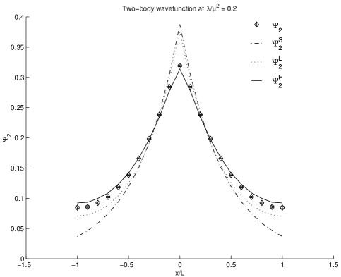
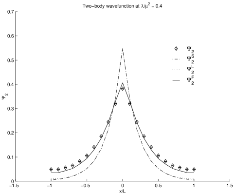
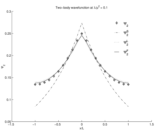
where |xket𝑥\left|x\right\rangle is the two-particle position state defined in (14).  In Figures 1-3 we compare the wavefunctions Ψ2subscriptΨ2\Psi_{2} with the corresponding approximate wavefunctions Ψ2SsuperscriptsubscriptΨ2S\Psi_{2}^{\text{S}}, Ψ2LsuperscriptsubscriptΨ2L\Psi_{2}^{\text{L}}, Ψ2FsuperscriptsubscriptΨ2F\Psi_{2}^{\text{F}} for coupling values λ=0.1μ2,0.2μ2,0.4μ2𝜆0.1superscript𝜇20.2superscript𝜇20.4superscript𝜇2\lambda=0.1\mu^{2},0.2\mu^{2},0.4\mu^{2}.

In our analysis we did not consider bound states beyond λ=0.6μ2𝜆0.6superscript𝜇2\lambda=0.6\mu^{2}.  This is because our diagonalization/Monte Carlo results indicate a first order phase transition near λ=0.73μ2𝜆0.73superscript𝜇2\lambda=0.73\mu^{2}, where ϕitalic-ϕ\phi develops a vacuum expectation value

ϕ=1.02(2).delimited-⟨⟩italic-ϕ1.022\left\langle\phi\right\rangle=1.02(2). (59)

As a matter of fact, there appears to be no bound state in the broken symmetry phase, and the two-body and three-body bound states in the symmetric phase are stable all the way up to the transition point. The phase transition can be seen quite clearly in the behavior of the energy levels.  In Table 3 we show the lowest two energy levels E0subscript𝐸0E_{0} and E2subscript𝐸2E_{2} in the even ϕitalic-ϕ\phi sector.  We see what appears to be a metastable vacuum at energy E2subscript𝐸2E_{2} for λ<0.73μ2𝜆0.73superscript𝜇2\lambda<0.73\mu^{2} becoming the true vacuum at energy E0subscript𝐸0E_{0} for λ>0.73μ2𝜆0.73superscript𝜇2\lambda>0.73\mu^{2}.333Since we are at finite volume the levels E0subscript𝐸0E_{0} and E2subscript𝐸2E_{2} come close but never actually become degenerate.

0.700.37(5)0.09(10)0.710.41(5)0.15(15)0.720.40(5)0.29(20)0.730.49(20)0.42(5)0.740.70(20)0.42(5)Table 3Table 3fragments 0.70fragments0.37(5)fragments0.09(10)0.71fragments0.41(5)fragments0.15(15)0.72fragments0.40(5)fragments0.29(20)0.73fragments0.49(20)fragments0.42(5)0.74fragments0.70(20)fragments0.42(5)\overset{\text{Table 3}}{\begin{tabular}[c]{|l|l|l|}\hline\cr$\lambda/\mu^{2}$&$E_{0}$&$E_{2}$\\ \hline\cr$0.70$&$-0.37(5)$&$0.09(10)$\\ \hline\cr$0.71$&$-0.41(5)$&$-0.15(15)$\\ \hline\cr$0.72$&$-0.40(5)$&$-0.29(20)$\\ \hline\cr$0.73$&$-0.49(20)$&$-0.42(5)$\\ \hline\cr$0.74$&$-0.70(20)$&$-0.42(5)$\\ \hline\cr\end{tabular}}
/λμ2E0E2/λμ2E0E2

In Table 4 we show for several values of λ𝜆\lambda the mass of the three-body bound state, m3subscript𝑚3m_{3}, which is the relativistic state that is continously connected to the non-relativistic three-body bound state.  We were not able to find any previous studies of this state in the literature.  For comparison we show data from the Schrödinger equation at infinite L𝐿L (S) and two different Fock space approximations, F1 and F2.  F1 corresponds with an exact diagonalization of the Hamiltonian restricted to three-particle Fock states, and F2 corresponds to the same thing, except with the :ϕ6::\phi^{6}: interaction turned off.444This is an artificial approximation.  Without the restriction to three-particle Fock states, turning off the :ϕ6::\phi^{6}: interaction would make the theory unbounded below.  To obtain the ratio m3/m1subscript𝑚3subscript𝑚1m_{3}/m_{1} in the two Fock approximations we again take m1=μ.subscript𝑚1𝜇m_{1}=\mu.

0.12.931(2)2.9102.9402.9190.22.83(1)2.6402.8622.7700.32.72(2)2.1902.7692.5680.42.59(6)1.5602.6672.3360.52.54(8)0.752.5582.0840.62.62(15)<02.4441.818Table 4Table 4fragments 0.1fragments2.931(2)2.9102.9402.9190.2fragments2.83(1)2.6402.8622.7700.3fragments2.72(2)2.1902.7692.5680.4fragments2.59(6)1.5602.6672.3360.5fragments2.54(8)0.752.5582.084fragments0.6fragments2.62(15)fragments02.4441.818\overset{\text{Table 4}}{\begin{tabular}[c]{|l|l|l|l|l|}\hline\cr$\lambda/\mu^{2}$&$m_{3}/m_{1}$&S&F${}_{1}$&F${}_{2}$\\ \hline\cr$0.1$&$2.931(2)$&$2.910$&$2.940$&$2.919$\\ \hline\cr$0.2$&$2.83(1)$&$2.640$&$2.862$&$2.770$\\ \hline\cr$0.3$&$2.72(2)$&$2.190$&$2.769$&$2.568$\\ \hline\cr$0.4$&$2.59(6)$&$1.560$&$2.667$&$2.336$\\ \hline\cr$0.5$&$2.54(8)$&$0.75$&$2.558$&$2.084$\\ \hline\cr$0.6$&$2.62(15)$&$<0$&$2.444$&$1.818$\\ \hline\cr\end{tabular}}
/λμ2/m3m1SF1 F2 /λμ2/m3m1SF1 F2

We notice that the Schrödinger approximation (S) is not quite as accurate for given λ𝜆\lambda as it was for the two-body bound state.  Nevertheless the Fock approximation F1 still appears to follow the actual data relatively well.  We observe that m3subscript𝑚3m_{3} is not only below the 3m13subscript𝑚13m_{1} continuum threshold but also below the m2+m1subscript𝑚2subscript𝑚1m_{2}+m_{1} threshold.  The corresponding state therefore has a sensible interpretation as a stable particle.

In analogy with before, we let |m3ketsubscript𝑚3\left|m_{3}\right\rangle be the normalized three-body bound state and P3subscript𝑃3P_{3} be the projection operator onto the three-particle subspace.  We define N3subscript𝑁3N_{3} to be the norm of the three-particle projection.

N3=P3|m3.subscript𝑁3normsubscript𝑃3ketsubscript𝑚3N_{3}=\left\|P_{3}\left|m_{3}\right\rangle\right\|. (60)

In Table 5 we show N3subscript𝑁3N_{3} for different couplings.

λ/μ20.10.20.30.40.50.6N30.9966(2)0.981(2)0.950(5)0.89(1)0.80(2)0.66(4)Table 5Table 5fragmentsλμ20.10.20.30.40.50.6fragmentsN3fragments0.9966(2)fragments0.981(2)fragments0.950(5)fragments0.89(1)fragments0.80(2)fragments0.66(4)\overset{\text{Table 5}}{\begin{tabular}[c]{|l|l|l|l|l|l|l|}\hline\cr$\lambda/\mu^{2}$&$0.1$&$0.2$&$0.3$&$0.4$&$0.5$&$0.6$\\ \hline\cr$N_{3}$&$0.9966(2)$&$0.981(2)$&$0.950(5)$&$0.89(1)$&$0.80(2)$&$0.66(4)$\\ \hline\cr\end{tabular}}

Let

Ψ3(x1,x2)=1N3x1,x2|m3.subscriptΨ3subscript𝑥1subscript𝑥21subscript𝑁3inner-productsubscript𝑥1subscript𝑥2subscript𝑚3\Psi_{3}(x_{1},x_{2})=\tfrac{1}{N_{3}}\left\langle x_{1},x_{2}\right|\left.m_{3}\right\rangle. (61)

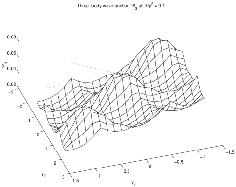
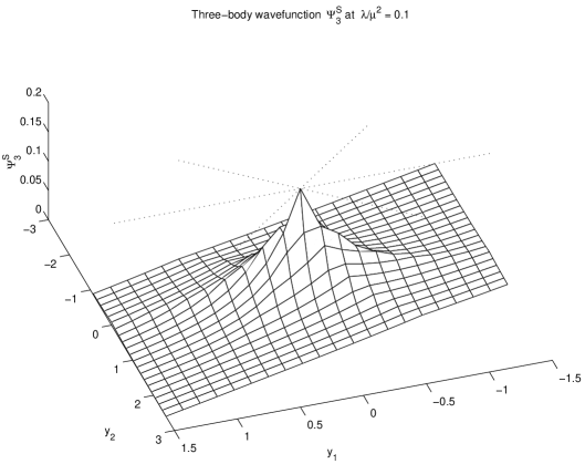
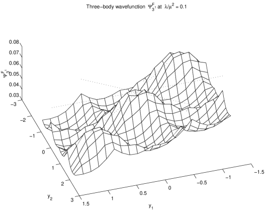
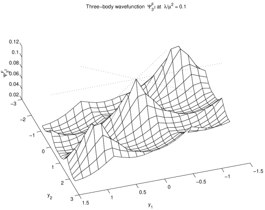
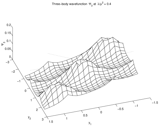
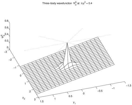
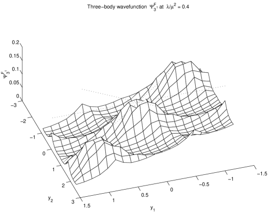
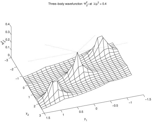
In Figures 4-11 we compare the wavefunction Ψ3subscriptΨ3\Psi_{3} with the corresponding approximate wavefunctions Ψ3SsuperscriptsubscriptΨ3S\Psi_{3}^{\text{S}}, Ψ3F1superscriptsubscriptΨ3subscriptF1\Psi_{3}^{\text{F}_{1}}, Ψ3F2superscriptsubscriptΨ3subscriptF2\Psi_{3}^{\text{F}_{2}} for λ=0.1μ2𝜆0.1superscript𝜇2\lambda=0.1\mu^{2} and 0.4μ20.4superscript𝜇20.4\mu^{2}.  For visual clarity we plot the wavefunctions over three copies of the fundamental region R𝑅R.  We use the variables

y1subscript𝑦1\displaystyle y_{1} =32Lx1,absent32𝐿subscript𝑥1\displaystyle=\tfrac{3}{2L}x_{1}, (62)
y2subscript𝑦2\displaystyle y_{2} =32L(x1+2x2),absent32𝐿subscript𝑥12subscript𝑥2\displaystyle=\tfrac{\sqrt{3}}{2L}\left(x_{1}+2x_{2}\right), (63)

to make clear the hexagon symmetry.  To guide the eye we have drawn dotted lines along the points

x1subscript𝑥1\displaystyle x_{1} =x2,absentsubscript𝑥2\displaystyle=x_{2}, (64)
x1subscript𝑥1\displaystyle x_{1} =x1x2,absentsubscript𝑥1subscript𝑥2\displaystyle=-x_{1}-x_{2}, (65)
x2subscript𝑥2\displaystyle x_{2} =x1x2.absentsubscript𝑥1subscript𝑥2\displaystyle=-x_{1}-x_{2}. (66)

These corresponds with configurations where two of the three constituents lie at the same point.

We notice that for both Ψ3subscriptΨ3\Psi_{3} and Ψ3F1,superscriptsubscriptΨ3subscriptF1\Psi_{3}^{\text{F}_{1}}, the inclusion of the repulsive :ϕ6::\phi^{6}: interaction produces a marked suppression of the wavefunction near the origin.  By independently changing the coefficients of :ϕ6::\phi^{6}: and :ϕ4::\phi^{4}:, we have a simple laboratory to study the competition between two-body and three-body forces in three-body bound states, a topic of some relevance and recent interest in the triton system. [10]
8 Summary

We have considered the relativistic bound states of ϕ6ϕ4superscriptitalic-ϕ6superscriptitalic-ϕ4\phi^{6}-\phi^{4} theory in 1+1111+1 dimensions.  Using a recently proposed diagonalization/Monte Carlo computational scheme, we calculated the two-body and three-body bound state energies and wavefunctions.  The initial diagonalization was performed using the quasi-sparse eigenvector method, and the subsequent stochastic error correction was calculated to first-order using the series method.  We made detailed comparisons of our numerical results with the available literature and several approximations, including non-relativistic weak-coupling solutions and various truncated Fock space approximations.

Applications to more complicated higher dimensional theories can be done in the same manner but require larger QSE subspaces and going beyond the first-order term in the series method or use of the stochastic Lanczos method.  But even from the simple examples presented here, the potential for studying relativistic bound states with diagonalization/Monte Carlo methods is apparent.

Acknowledgments


Financial support provided by the DFG and NSF.

References

  • [1] D. J. Lee, N. Salwen, D. D. Lee, hep-th/0002251.
  • [2] D. Lee, N. Salwen, M. Windoloski, hep-lat/0010039.
  • [3] J. Glimm, A. Jaffe, T. Spencer, Constructive quantum field theory, Proc. 1973 Ettore Majorana Inter. School of Math. Phys. (Springer, Berlin, 1973) 165.
  • [4] D. Lee, cond-mat/0008457; N. Salwen, cond-mat/0008458.
  • [5] P. Marrero, E. Roura, D. Lee, Phys. Lett. 471B (1999) 45.
  • [6] J. Dimock, J.-P. Eckmann, Commun. Math. Phys. 51 (1976) 41.
  • [7] T. Barnes, G. Daniell, Phys. Lett. 142B (1984) 188; Phys. Rev. D28 (1983) 2045.
  • [8] J. Darewych, M. Horbatsch, R. Koniuk, Phys. Rev. Lett. 54 (1985) 2188.
  • [9] P. Stevenson, Phys. Rev. D30 (1984) 1712; P. Stevenson, Phys. Rev. D32 (1985) 1389; P. Stevenson, I. Roditi, Phys.Rev. D33 (1986) 2305.
  • [10] P. Bedaque, H.-W. Hammer, U. van Kolck, Nucl. Phys. A676 (2000) 357.
Refer to caption
Figure 1: Two-body wavefunction Ψ2subscriptΨ2\Psi_{2} and approximate wavefunctions Ψ2S,Ψ2L,Ψ2FsuperscriptsubscriptΨ2SsuperscriptsubscriptΨ2LsuperscriptsubscriptΨ2F\Psi_{2}^{\text{S}},\Psi_{2}^{\text{L}},\Psi_{2}^{\text{F}} at λ=0.1μ2.𝜆0.1superscript𝜇2\lambda=0.1\mu^{2}.
Refer to caption
Figure 2: Two-body wavefunction Ψ2subscriptΨ2\Psi_{2} and approximate wavefunctions Ψ2S,Ψ2L,Ψ2FsuperscriptsubscriptΨ2SsuperscriptsubscriptΨ2LsuperscriptsubscriptΨ2F\Psi_{2}^{\text{S}},\Psi_{2}^{\text{L}},\Psi_{2}^{\text{F}} at λ=0.2μ2.𝜆0.2superscript𝜇2\lambda=0.2\mu^{2}.
Refer to caption
Figure 3: Two-body wavefunction Ψ2subscriptΨ2\Psi_{2} and approximate wavefunctions Ψ2S,Ψ2L,Ψ2FsuperscriptsubscriptΨ2SsuperscriptsubscriptΨ2LsuperscriptsubscriptΨ2F\Psi_{2}^{\text{S}},\Psi_{2}^{\text{L}},\Psi_{2}^{\text{F}} at λ=0.4μ2.𝜆0.4superscript𝜇2\lambda=0.4\mu^{2}.
Refer to caption
Figure 4: Three-body wavefunction Ψ3subscriptΨ3\Psi_{3} at λ=0.1μ2.𝜆0.1superscript𝜇2\lambda=0.1\mu^{2}.
Refer to caption
Figure 5: Approximate three-body wavefunction Ψ3SsuperscriptsubscriptΨ3S\Psi_{3}^{\text{S}} at λ=0.1μ2.𝜆0.1superscript𝜇2\lambda=0.1\mu^{2}.
Refer to caption
Figure 6: Approximate three-body wavefunction Ψ3F1superscriptsubscriptΨ3subscriptF1\Psi_{3}^{\text{F}_{1}} at λ=0.1μ2.𝜆0.1superscript𝜇2\lambda=0.1\mu^{2}.
Refer to caption
Figure 7: Approximate three-body wavefunction Ψ3F2superscriptsubscriptΨ3subscriptF2\Psi_{3}^{\text{F}_{2}} at λ=0.1μ2.𝜆0.1superscript𝜇2\lambda=0.1\mu^{2}.
Refer to caption
Figure 8: Three-body wavefunction Ψ3subscriptΨ3\Psi_{3} at λ=0.4μ2.𝜆0.4superscript𝜇2\lambda=0.4\mu^{2}.
Refer to caption
Figure 9: Approximate three-body wavefunction Ψ3SsuperscriptsubscriptΨ3S\Psi_{3}^{\text{S}} at λ=0.4μ2.𝜆0.4superscript𝜇2\lambda=0.4\mu^{2}.
Refer to caption
Figure 10: Approximate three-body wavefunction Ψ3F1superscriptsubscriptΨ3subscriptF1\Psi_{3}^{\text{F}_{1}} at λ=0.4μ2.𝜆0.4superscript𝜇2\lambda=0.4\mu^{2}.
Refer to caption
Figure 11: Approximate three-body wavefunction Ψ3F2superscriptsubscriptΨ3subscriptF2\Psi_{3}^{\text{F}_{2}} at λ=0.4μ2.𝜆0.4superscript𝜇2\lambda=0.4\mu^{2}.