IPPP/00/04

DTP/00/64

MSUHEP-01024

DFTT 44/2000

Mueller-Navelet Jets at Hadron Colliders

J. R. Andersen¹, V. Del Duca², S. Frixione³, C.R. Schmidt⁴ and W.J. Stirling¹

¹Institute for Particle Physics Phenomenology
University of Durham
Durham, DH1 3LE, U.K.

²I.N.F.N., Sezione di Torino
via P. Giuria, 1 - 10125 Torino, Italy

³I.N.F.N., Sezione di Genova
via Dodecaneso, 33 - 16146 Genova, Italy

⁴Department of Physics and Astronomy
Michigan State University
East Lansing, MI 48824, USA

We critically examine the definition of dijet cross sections at large rapidity intervals in hadron–hadron collisions, taking proper account of the various cuts applied in a realistic experimental setup. We argue that the dependence of the cross section on the precise definition of the parton momentum fractions and the presence of an upper bound on the momentum transfer cannot be neglected, and we provide the relevant modifications to the analytical formulae by Mueller and Navelet. We also point out that the choice of equal transverse momentum cuts on the tagging jets can spoil the possibility of a clean extraction of signals of BFKL physics.

1 Introduction

Long ago Mueller and Navelet suggested [1] to look for evidence of Balitsky-Fadin-Kuraev-Lipatov (BFKL) evolution [2, 3, 4] by measuring dijet cross section at hadron colliders as a function of the hadronic centre-of-mass energy $\sqrt{S}$, at fixed momentum fractions $x_{a,b}$ of the incoming partons. This is equivalent to measuring the rates as a function of the rapidity interval $\Delta y=|y_{a}-y_{b}|$ between the jets. In fact, at large enough rapidities, the rapidity interval is well approximated by the expression $\Delta y\simeq\ln(\hat{s}/|\hat{t}|)$, where $\hat{s}=x_{a}x_{b}S$ and $|\hat{t}|\simeq\mbox{$k_{a\perp}$}\mbox{$k_{b\perp}$}$, with $k_{a,b\perp}$ being the moduli of the transverse momenta (i.e., the transverse energies) of the two jets. Thus, since the cross section tends to peak at the smallest available transverse energies, $\Delta y$ grows as $\ln S$ at fixed $x_{a,b}$.

It is clear that the measurement proposed by Mueller and Navelet is not feasible at a collider run at a fixed energy; on the other hand, to look for the BFKL-driven rise of the parton cross section directly in the dijet production rate $d\sigma/\Delta y$ as a function of $\Delta y$ is difficult due to the steep fall-off of the parton densities [5, 6]. This led some of us to propose the study of less inclusive observables. In particular, the angular correlation between the tagged jets, which at leading order (LO) are back-to-back, is smeared by gluon radiation and by hadronization. Part of the gluon radiation originates from the mechanism responsible for BFKL effects, namely from gluon radiation in the rapidity interval between the jets. Accordingly, the transverse momentum imbalance [5, 7] and the azimuthal angle decorrelation [5, 6, 8, 9, 10] have been proposed as observables sensitive to BFKL effects. The azimuthal angle decorrelation has indeed been studied by the D0 Collaboration at the Tevatron Collider [11]. As expected, a NLO partonic Monte Carlo generator, JETRAD [12, 13], predicts too little decorrelation. However, the BFKL formalism predicts a much stronger decorrelation than that observed in the data. In fact, the data are well described by the HERWIG Monte Carlo generator [14, 15, 16], which dresses the basic $2\to 2$ parton scattering with parton showers and hadronization. This hints at a description of the azimuthal angle decorrelation in terms of a standard Sudakov resummation [17]. It therefore appears that, in the presence of Sudakov logarithms, it is quite difficult to cleanly extract the presence of BFKL logarithms from this observable, not least because the latter are expected to be smaller than the former in the energy range explored at present. It thus comes as no surprise that D0 Collaboration [11] find no strong evidence of BFKL effects in their data.

Recently, the D0 Collaboration [18] has revisited the original Mueller-Navelet proposal, and has measured the ratio

$$R={\sigma(\sqrt{S_{{}_{A}}})\over\sigma(\sqrt{S_{{}_{B}}})}$$ (1.1)

of dijet cross sections obtained at two different centre-of-mass energies, $\sqrt{S_{{}_{A}}}=1800$ GeV and $\sqrt{S_{{}_{B}}}=630$ GeV. The dijet events have been selected by tagging the most forward/backward jets in the event, and the cross section is measured as a function of the momentum transfer, defined as $Q^{2}=\mbox{$k_{a\perp}$}\mbox{$k_{b\perp}$}$, and of the quantities

$$x_{1}=\frac{2\mbox{$k_{a\perp}$}}{\sqrt{S}}e^{\bar{y}}\cosh(\Delta y/2)\,,\qquad x_{2}=\frac{2\mbox{$k_{b\perp}$}}{\sqrt{S}}e^{-\bar{y}}\cosh(\Delta y/2)\,,$$ (1.2)

with $\bar{y}=(y_{a}+y_{b})/2$, $\Delta y=y_{a}-y_{b}\geq 0$, and $y_{a}$ ($y_{b}$) are the rapidities of the most forward (backward) jet. The dimensionless quantities $x_{1}$ and $x_{2}$ are reconstructed from the tagged jets using Eq. (1.2), irrespective of the number of additional jets in the final state. In leading-order kinematics, for which only two (back-to-back) jets are present in the final state, we have $x_{1}=x_{a}$ and $x_{2}=x_{b}$, the momentum fractions of the incoming partons. Higher-order corrections entail that these equalities no longer hold; however, $x_{1}=x_{a}$ and $x_{2}=x_{b}$ are still reasonable approximations (unless one goes too close to the borders of phase space). This implies that when the ratio in Eq. (1.1) is computed at fixed $x_{1}$ and $x_{2}$, the contributions due to the parton densities cancel to a large extent, thus giving the possibility of studying BFKL effects without any contamination from long-distance phenomena.

	$x_{1}$ range	$x_{2}$ range
bin 1	0.06-0.10	0.18-0.22
bin 2	0.10-0.14	0.14-0.18
bin 3	0.10-0.14	0.18-0.22
bin 4	0.14-0.18	0.14-0.18
bin 5	0.14-0.18	0.18-0.22
bin 6	0.18-0.22	0.18-0.22

Table 1: ($x_{1},x_{2}$) bins, with the upper bound of range in $x_{1}$ not larger than the upper bound of the range in $x_{2}$.

In the analysis performed by D0 [18], jets have been selected by requiring $k_{a,b\perp}>20$ GeV, $|y_{a,b}|<3$, and $\Delta y>2$. The cross section was measured for ten ($x_{1},x_{2}$) bins, of which we list in Table 1 the six with the upper bound of the range in $x_{1}$ smaller than or equal to the upper bound of the range in $x_{2}$ (the others may be obtained by interchanging $x_{1}\leftrightarrow x_{2}$). Finally, a cut on the momentum transfer, $400<Q^{2}<1000$ GeV², has been imposed. With larger statistics, a binning in $Q^{2}$ would also be possible. These cuts select dijet events at large rapidity intervals. To have a crude estimate of the typical $\Delta y$ values involved, we observe that, in a given $(x_{1},x_{2})$ bin, the data accumulate at the minimum $x_{1}$ and $x_{2}$ in order to maximise the parton luminosity, and at minimum $k_{\perp}$ in order to maximise the partonic cross section. We can then use the LO kinematics (1.2) to obtain the effective rapidity interval. For instance, in bin 5 we find $\Delta y_{{}_{A}}\simeq 5.3$ at $\sqrt{S_{{}_{A}}}$=1800 GeV, and $\Delta y_{{}_{B}}\simeq 3.1$ at $\sqrt{S_{{}_{B}}}=630$ GeV. In addition, we see that in the large–$\Delta y$ limit, $\Delta y_{{}_{A}}\to\Delta y_{{}_{B}}+\ln(S_{{}_{A}}/S_{{}_{B}})$.

The data collected by D0 are compared to BFKL predictions as given by Mueller and Navelet, and an effective ‘BFKL intercept’ is then extracted (see Eq. (2.16) below). However, we argue in this paper that the different reconstruction of the $x$’s used by D0 as compared to the original Mueller-Navelet analysis (see Eqs. (1.2) and (2.11)), and some of the acceptance cuts imposed in the experimental analysis, like the introduction of an upper bound on the momentum transfer $Q^{2}$, actually spoil the correctness of this procedure, and require modifications of the Mueller-Navelet formulae. These modifications are subleading from the standpoint of the BFKL theory, however they have an impact on the extraction of the BFKL intercept at subasymptotic energies. Furthermore, the fact that dijet events are selected by means of transverse momentum cuts which are the same for the two tagged jets poses additional problems: large logarithms of (non-BFKL) perturbative origin enter the cross section, and thus the ratio of Eq. (1.1) is affected by the same kind of problems as the azimuthal decorrelation.

In this study we address the quantitative importance of these issues on the D0 analysis using a combination of analytic and numerical techniques and several different theoretical approximations for dijet production. The paper is organized as follows: in Section 2, we study the impact of a different definition of the $x$’s and of the upper bound on $Q^{2}$ in the framework of the naive BFKL equation, and compare the result with the standard Mueller-Navelet analysis. In Section 3, our BFKL predictions are refined by considering running-coupling effects, and implementing energy-momentum conservation; this is done by using Monte Carlo techniques. In Section 4 the problem of equal transverse momentum cuts is investigated; in Subsection 4.1 we use a fixed-order perturbative computation (accurate to NLO), and in Subsection 4.2 we return to the BFKL formalism. Finally, Section 5 reports on our conclusions.

2 Dijet production at fixed $x$’s in the naive BFKL approach

In large-rapidity dijet production, the rapidity interval is related to the kinematic invariants through $\Delta y\simeq\ln(\hat{s}/|\hat{t}|)$, with $\hat{s}$ the squared parton centre-of-mass energy and $|\hat{t}|$ of the order of the squared jet transverse energy. Thus, in computing the dijet production rate we encounter large logarithms, which arise in a perturbative calculation at each order in the coupling constant $\alpha_{s}$. The large logarithms can be resummed in leading-logarithmic (LL) approximation through the BFKL equation.

In the high-energy limit, $\hat{s}\gg|\hat{t}|$, the BFKL theory assumes that any scattering process is dominated by gluon exchange in the crossed channel. This constitutes the leading (LL) term of the BFKL resummation. The corresponding QCD amplitude factorizes into a gauge-invariant effective amplitude formed by two scattering centres, the LO impact factors, connected by the gluon exchanged in the crossed channel. The BFKL equation then resums the universal LL corrections, of ${\cal O}(\alpha_{s}^{n}\ln^{n}(\hat{s}/|\hat{t}|))$, to the gluon exchange in the crossed channel. These are obtained in the limit of strong rapidity ordering of the emitted gluon radiation, i.e. for $n+2$ gluons produced in the scattering,

$$y_{a}\gg y_{1}\gg y_{2}\gg\ldots\gg y_{n-1}\gg y_{n}\gg y_{b}\,.$$ (2.1)

In dijet production at large rapidity intervals, the crossed-channel gluon dominance  ensures that the functional form of the QCD amplitudes for gluon-gluon, gluon-quark or quark-quark scattering at LO is the same; they differ only by the colour strength in the parton-production vertices. We can then write the cross section in the following factorized form [1]

$${d\sigma\over dx_{a}^{0}dx_{b}^{0}}\,=\,\int d\mbox{$k_{a\perp}^{2}$}d\mbox{$k_{b\perp}^{2}$}f_{\rm eff}(x_{a}^{0},\mbox{$\mu_{\scriptscriptstyle F}^{2}$})\,f_{\rm eff}(x_{b}^{0},\mbox{$\mu_{\scriptscriptstyle F}^{2}$})\,{d\hat{\sigma}_{gg}\over d\mbox{$k_{a\perp}^{2}$}d\mbox{$k_{b\perp}^{2}$}}\,,$$ (2.2)

where $\mu_{\scriptscriptstyle F}$ is the factorization scale, and $x_{a}^{0},\,x_{b}^{0}$ are the parton momentum fractions (1.2) in the high-energy limit,

$$x_{a}^{0}=\frac{\mbox{$k_{a\perp}$}}{\sqrt{S}}e^{y_{a}}\qquad\qquad x_{b}^{0}=\frac{\mbox{$k_{b\perp}$}}{\sqrt{S}}e^{-y_{b}}\,,$$ (2.3)

and the effective parton densities are [24]

$$f_{\rm eff}(x,\mbox{$\mu_{\scriptscriptstyle F}^{2}$})=G(x,\mbox{$\mu_{\scriptscriptstyle F}^{2}$})+{4\over 9}\sum_{f}\left[Q_{f}(x,\mbox{$\mu_{\scriptscriptstyle F}^{2}$})+\bar{Q}_{f}(x,\mbox{$\mu_{\scriptscriptstyle F}^{2}$})\right],$$ (2.4)

where the sum runs over the quark flavours. In the high-energy limit, the azimuthally-averaged gluon-gluon scattering cross section becomes [1]

$${d\hat{\sigma}_{gg}\over d\mbox{$k_{a\perp}^{2}$}d\mbox{$k_{b\perp}^{2}$}}\ =\ \biggl{[}{C_{A}\alpha_{s}\over\mbox{$k_{a\perp}^{2}$}}\biggr{]}\,{\bar{f}}(\mbox{$q_{a\perp}$},\mbox{$q_{b\perp}$},\Delta y)\,\biggl{[}{C_{A}\alpha_{s}\over\mbox{$k_{b\perp}^{2}$}}\biggr{]}\ ,$$ (2.5)

where $C_{A}=N_{c}=3$, and $q_{a\perp}$, $q_{b\perp}$ are the momenta transferred in the $t$-channel, with $\vec{q}_{a\perp}=-\mbox{$\vec{k}_{a\perp}$}$ and $\vec{q}_{b\perp}=\mbox{$\vec{k}_{b\perp}$}$. The quantities in square brackets are the LO impact factors for jet production. The function ${\bar{f}}(\mbox{$q_{a\perp}$},\mbox{$q_{b\perp}$},\Delta y)$ is the azimuthally-averaged Green’s function associated with the gluon exchanged in the crossed channel, and is obtained by integrating out the azimuthal angles in the solution of the BFKL equation,

$${\bar{f}}(\mbox{$q_{a\perp}$},\mbox{$q_{b\perp}$},\Delta y)\,={1\over 4\sqrt{\mbox{$q_{a\perp}^{2}$}\mbox{$q_{b\perp}^{2}$}}}\int_{-\infty}^{\infty}d\nu\,e^{\omega(\nu)\Delta y}\,\left(\mbox{$q_{a\perp}^{2}$}\over\mbox{$q_{b\perp}^{2}$}\right)^{i\nu}\,,$$ (2.6)

with

$$\omega(\nu) = -2{\bar{\alpha}_{s}}\,\left[{\rm Re}\,\psi\left(1/2+i\nu\right)-\psi(1)\right]$$ (2.7)

$$= A-B\nu^{2}+{\cal O}(\nu^{4})\,,$$ (2.8)

with $\psi$ the digamma function, and

$$\bar{\alpha}_{s}\,=\,\alpha_{s}N_{c}/\pi,\;\;\;\;A\,=\,4\bar{\alpha}_{s}\ln{2},\;\;\;\;B\,=\,14\zeta(3)\,\bar{\alpha}_{s},$$ (2.9)

2.1 The standard Mueller-Navelet analysis

In order to elucidate how the D0 Collaboration [18] evaluates the effective BFKL intercept, we follow the original Mueller-Navelet approach [1], i.e. we substitute Eqs. (2.5) and (2.6) into Eq. (2.2) and integrate it over the transverse momenta $k_{a\perp}$ and $k_{b\perp}$ above a threshold $E_{\perp}$, at fixed coupling $\alpha_{s}$ and fixed $x_{a}^{0},\,x_{b}^{0}$. The rapidity interval $\Delta y=|y_{a}-y_{b}|$ in Eq. (2.6) is determined from the $x$’s (2.3),

$$\Delta y=\ln{x_{a}^{0}x_{b}^{0}S\over\mbox{$k_{a\perp}$}\mbox{$k_{b\perp}$}}$$ (2.10)

and since it depends on $k_{a\perp}$$k_{b\perp}$, it is not a constant within the integral. However, the dominant, i.e. the leading logarithmic, contribution to Eq. (2.6) comes from the largest value of $\Delta y$, which is attained at the transverse momentum threshold, thus in Ref. [1] $\Delta y$ is fixed at its maximum by reconstructing the $x$’s at the kinematic threshold for jet production and setting them in a one-to-one correspondence with the jet rapidities

$$x_{a}^{\scriptscriptstyle{\rm MN}}=\frac{\mbox{$E_{\perp}$}}{\sqrt{S}}e^{y_{a}}\qquad\qquad x_{b}^{\scriptscriptstyle{\rm MN}}=\frac{\mbox{$E_{\perp}$}}{\sqrt{S}}e^{-y_{b}}\,.$$ (2.11)

Then the factorization formula (2.2) is determined at fixed $x_{a}^{\scriptscriptstyle{\rm MN}},x_{b}^{\scriptscriptstyle{\rm MN}}$. Having fixed the rapidity interval (2.10) to

$$\Delta y=\ln{x_{a}^{\scriptscriptstyle{\rm MN}}x_{b}^{\scriptscriptstyle{\rm MN}}S\over\mbox{$E_{\perp}^{2}$}}\,,$$ (2.12)

the integration over $k_{a\perp}$ and $k_{b\perp}$ can be straightforwardly performed, and the gluon-gluon cross section (2.5) becomes

$$\hat{\sigma}_{gg}(\mbox{$k_{a\perp}$}\!>\!\mbox{$E_{\perp}$},\mbox{$k_{b\perp}$}\!>\!\mbox{$E_{\perp}$})\,={\pi C_{A}^{2}\alpha_{s}^{2}\over 2\mbox{$E_{\perp}^{2}$}}{\cal F}(\Delta y,1)\,,$$ (2.13)

with

$${\cal F}(z,t)={1\over 2\pi}\int_{-\infty}^{\infty}d\nu\,{e^{\omega(\nu)z}\over\nu^{2}+1/4}\,\cos(2\nu\ln t)\,.$$ (2.14)

For $\bar{\alpha}_{s}\Delta y\ll 1$, we can expand Eq. (2.14) and obtain [1]

$$\hat{\sigma}_{gg}(\mbox{$k_{a\perp}$}\!>\!\mbox{$E_{\perp}$},\mbox{$k_{b\perp}$}\!>\!\mbox{$E_{\perp}$})\,={\pi C_{A}^{2}\alpha_{s}^{2}\over 2\mbox{$E_{\perp}^{2}$}}\left[1+{\cal O}\left((\bar{\alpha}_{s}\Delta y)^{2}\right)\right]\,.$$ (2.15)

On the other hand, for $\Delta y\gg 1$ we can perform a saddle-point evaluation of Eq. (2.14), and using the small-$\nu$ expansion (2.8), we obtain the asymptotic behaviour of the gluon-gluon cross section [3, 4]

$$\hat{\sigma}_{gg}^{(\Delta y\gg 1)}(\mbox{$k_{a\perp}$}\!>\!\mbox{$E_{\perp}$},\mbox{$k_{b\perp}$}\!>\!\mbox{$E_{\perp}$})\,={\pi C_{A}^{2}\alpha_{s}^{2}\over 2\mbox{$E_{\perp}^{2}$}}{e^{A\Delta y}\over\sqrt{\pi B\Delta y/4}}\,.$$ (2.16)

At very large rapidities the resummed gluon-gluon cross section grows exponentially with $\Delta y$, in contrast to the LO (${\cal O}(\alpha_{s}^{2})$) cross section (2.15), which is constant at large $\Delta y$. From the asymptotic formula (2.16) the effective BFKL intercept $\alpha_{\scriptscriptstyle BFKL}\equiv A+1$ can be derived. In the experiment of Ref. [18] the BFKL intercept is measured by considering the ratio of hadronic cross sections, Eq. (2.2), obtained at different centre-of-mass energies and at fixed $x_{1,2}$ and scale. This allows the dependence on the parton densities to cancel, and the ratio of hadronic cross sections is therefore approximately equal to that of partonic cross sections evaluated at the relevant $\Delta y$ values.

In Eqs. (2.13)–(2.16) we have summarised the standard Mueller-Navelet analysis in which it is assumed that the $x$’s are reconstructed through Eq. (2.11), and that the jet transverse momenta are unbounded from above. However, this is not the case for the D0 analysis, since

• D0 collect data with an upper bound on $Q^{2}=\mbox{$k_{a\perp}$}\mbox{$k_{b\perp}$}$, which is of the same order of magnitude as the square of the lower cut on the jet transverse momenta, and thus cannot be ignored in the integration over the transverse momenta.

• D0 reconstruct the $x$’s through Eq. (1.2), which is well approximated by Eq. (2.3), but not by Eq. (2.11);

We examine these two issues, and the modifications they entail on Eqs. (2.13)–(2.16), in turn.

2.2 Dijet production with an upper bound on $Q^{2}$

In the Mueller-Navelet analysis the integration over the transverse momenta is taken up to infinity on the grounds that a finite and large upper bound on the transverse momenta would entail a contribution which is power suppressed in the ratio of the jet threshold to the upper bound. However, D0 collect data with an upper bound on $Q^{2}=\mbox{$k_{a\perp}$}\mbox{$k_{b\perp}$}$, namely $Q^{2}_{\rm max}$ = 1000 ${\rm GeV}^{2}$, while $Q^{2}_{\rm min}=\mbox{$E_{\perp}^{2}$}$ = 400 ${\rm GeV}^{2}$. When $Q^{2}_{\rm min}\sim Q^{2}_{\rm max}$, the upper bound cannot be ignored in the integration over the transverse momenta.

In order to assess what the modification on Eqs. (2.13)–(2.16) is, we integrate the gluon-gluon cross section (2.5) over the transverse momenta $k_{a\perp}$ and $k_{b\perp}$ above a threshold $E_{\perp}$ with the upper cut $Q^{2}<Q^{2}_{\rm max}$ imposed. We obtain

$$\hat{\sigma}_{gg}(\mbox{$k_{a\perp}$}\!>\!\mbox{$E_{\perp}$},\mbox{$k_{b\perp}$}\!>\!\mbox{$E_{\perp}$},\mbox{$k_{a\perp}$}\mbox{$k_{b\perp}$}\!\!<Q^{2}_{\rm max})={\pi C_{A}^{2}\alpha_{s}^{2}\over 2\mbox{$E_{\perp}^{2}$}}\left[{\cal F}(\Delta y,1)-{\mbox{$E_{\perp}^{2}$}\over Q^{2}_{\rm max}}{\cal G}\left(\Delta y,{\mbox{$E_{\perp}^{2}$}\over Q^{2}_{\rm max}}\right)\right]\,,$$ (2.17)

with rapidity interval $\Delta y$ defined in Eq. (2.12), ${\cal F}$ defined in Eq. (2.14), and

$${\cal G}(z,t)={\cal F}(z,t)-{1\over 2\pi}\int_{-\infty}^{\infty}d\nu\,{e^{\omega(\nu)z}\over\nu^{2}+1/4}{\sin\left(2\nu\ln{t}\right)\over 2\nu}\,.$$ (2.18)

The analytic form of Eq. (2.17) depends on the particular definition of the upper cutoff $Q^{2}_{\rm max}$ that D0 uses, and changes substantially the shape of the gluon-gluon cross section (see Fig. 1) and in particular its subasymptotic dependence on $\Delta y$. At $\bar{\alpha}_{s}\Delta y\ll 1$, we expand the exponentials in Eq. (2.17) and obtain

$$\hat{\sigma}_{gg}(\mbox{$k_{a\perp}$}\!>\!\mbox{$E_{\perp}$},\mbox{$k_{b\perp}$}\!>\!\mbox{$E_{\perp}$},\mbox{$k_{a\perp}$}\mbox{$k_{b\perp}$}\!\!<Q^{2}_{\rm max})\,={\pi C_{A}^{2}\alpha_{s}^{2}\over 2\mbox{$E_{\perp}^{2}$}}\left[1-{\mbox{$E_{\perp}^{2}$}\over Q^{2}_{\rm max}}+{\cal O}\left(\bar{\alpha}_{s}\Delta y\right)\right]\,.$$ (2.19)

Thus for the D0 cuts, $Q^{2}_{\rm max}$ = 1000 ${\rm GeV}^{2}$, Eq. (2.19) lowers the LO cross section (2.15) by 40%. At $\Delta y\gg 1$ a saddle-point evaluation of Eq. (2.17) yields

$$\hat{\sigma}_{gg}^{(\Delta y\gg 1)}(\mbox{$k_{a\perp}$}\!>\!\mbox{$E_{\perp}$},\mbox{$k_{b\perp}$}\!>\!\mbox{$E_{\perp}$},\mbox{$k_{a\perp}$}\mbox{$k_{b\perp}$}\!\!<Q^{2}_{\rm max})\ =\ {\pi C_{A}^{2}\alpha_{s}^{2}\over 2\mbox{$E_{\perp}^{2}$}}\ e^{A\Delta y}$$

$$\times \Biggl{\{}e^{B\Delta y/4}\left[\Phi\left({\ln(Q^{2}_{\rm max}/\mbox{$E_{\perp}^{2}$})+B\Delta y/2\over\sqrt{B\Delta y}}\right)-\Phi\left({\sqrt{B\Delta y}\over 2}\right)\right]-{\mbox{$E_{\perp}^{2}$}\over Q^{2}_{\rm max}}\Phi\left({\ln(Q^{2}_{\rm max}/\mbox{$E_{\perp}^{2}$})\over\sqrt{B\Delta y}}\right)\Biggr{\}}\,,$$

with the error function

$$\Phi(x)={2\over\sqrt{\pi}}\int_{0}^{x}dte^{-t^{2}}\,.$$ (2.21)

Using the asymptotic expansion of the error function at $x\gg$ 1, for very large rapidities $\sqrt{B\Delta y}\gg$ 1 and at fixed $Q^{2}_{\rm max}/\mbox{$E_{\perp}^{2}$}$ we obtain

$$\hat{\sigma}_{gg}^{(\Delta y\gg 1)}(\mbox{$k_{a\perp}$}\!>\!\mbox{$E_{\perp}$},\mbox{$k_{b\perp}$}\!>\!\mbox{$E_{\perp}$},\mbox{$k_{a\perp}$}\mbox{$k_{b\perp}$}\!\!<Q^{2}_{\rm max})\,={\pi C_{A}^{2}\alpha_{s}^{2}\over 2\mbox{$E_{\perp}^{2}$}}{e^{A\Delta y}\over\sqrt{\pi B\Delta y/4}}\left[1-{\mbox{$E_{\perp}^{2}$}\over Q^{2}_{\rm max}}\left(1+\ln{Q^{2}_{\rm max}\over\mbox{$E_{\perp}^{2}$}}\right)\right],$$ (2.22)

which is simply the asymptotic cross section of Eq. (2.16) reduced by a constant factor. For the D0 values of $E_{\perp}^{2}$ and $Q^{2}_{\rm max}$, this corresponds to a reduction by a factor of about 4.3 in the standard asymptotic formula (2.16).

Although it might appear from Eq. (2.22) that the only effect of the $Q^{2}_{\rm max}$ cut is to change the normalization relative to Eq. (2.16), which would drop out of the ratio of cross sections, one has to keep in mind that both equations are derived (from Eqs. (2.17) and (2.13) respectively) in the asymptotic limit $\Delta y\gg 1$. In Fig. 1 we plot both the integral formulae and their asymptotic solutions. We see that the differences $\hat{\sigma}_{gg}-\hat{\sigma}_{gg}^{(\Delta y\gg 1)}$ are roughly constant with respect to $\Delta y$, and thus the relative differences get smaller with increasing $\Delta y$. However, at the $\Delta y$ values relevant to D0 analysis, it appears that non-negligible subleading corrections to the asymptotic formulae should be taken into account when determining the effective BFKL intercept. As can be inferred from Fig. 1, these effects are more important when a $Q^{2}$ cut is imposed, since in this case it takes longer for the exponential rise with $\Delta y$ to set in.

In conclusion, the effect of an upper bound on the product of the jet transverse momenta can have a significant effect on both the normalization and $\Delta y$ dependence of the gluon-gluon cross section. For the D0 values, the increase of the cross section from small to large $\Delta y$ is weakened by a factor of approximately 2, as shown in Fig. 1. Care must therefore be taken in attributing any observed cross section increase exclusively to the $e^{A\Delta y}$ ‘BFKL’ factor.

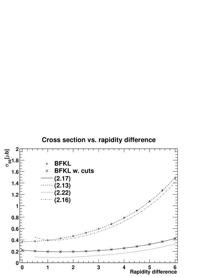
Figure 1: The dependence of the LL BFKL gluon-gluon subprocess cross section on the dijet rapidity separation $\Delta y$, without (Eq. (2.13), upper dashed line) and with (Eq. (2.17), lower solid line) the $Q^{2}_{\rm max}$ cut. The ‘data points’ are the same quantities calculated using the BFKL Monte Carlo discussed in Section 3, with $\alpha_{s}$ fixed and no additional kinematic cuts. Also shown are the asymptotic $\Delta y\gg 1$ approximations, Eqs. (2.16) and (2.22). The parameter values are $\alpha_{s}=0.164$, $\mbox{$E_{\perp}$}=20$ GeV, $Q^{2}_{\rm max}=1000$ GeV².

2.3 Dijet production at $x$’s fixed as in the D0 set-up

In the analysis performed by D0, the $x$’s are reconstructed through Eq. (1.2). Since the jets are selected by requiring that $\Delta y>2$, Eq. (2.3) is a good approximation to Eq. (1.2). Conversely, the $x$’s (2.11) used in the Mueller-Navelet analysis are by definition a good approximation to the D0 $x$’s (1.2) only at the kinematic threshold for jet production. Therefore in this section we shall examine the modifications induced on Eqs. (2.13)–(2.16) by defining the $x$’s as in Eq. (2.3). First, we note that in this case the jet rapidities are not fixed, rather in a given ($x_{a}^{0},\,x_{b}^{0}$) bin all the transverse momenta and rapidities contribute which fulfil Eq. (2.3). Thus the rapidity interval between the jets cannot be used as an independent, fixed observable. For convenience, we rewrite the rapidity interval (2.10) as

$$\Delta y=Y+\ln{\mbox{$E_{\perp}^{2}$}\over\mbox{$k_{a\perp}$}\mbox{$k_{b\perp}$}}\,,$$ (2.23)

with

$$Y=\ln{x_{a}^{0}x_{b}^{0}S\over\mbox{$E_{\perp}^{2}$}}\,.$$ (2.24)

The requirement that the rapidity interval be positive, $\Delta y\geq 0$, imposes an effective upper bound on $Q^{2}$,

$$Q^{2}_{\rm max}=\mbox{$E_{\perp}^{2}$}e^{Y}\,.$$ (2.25)

Integrating then the gluon-gluon cross section (2.5) over $k_{a\perp}$ and $k_{b\perp}$ above $E_{\perp}$, at fixed $x_{a}^{0},\,x_{b}^{0}$ and fixed coupling $\alpha_{s}$, we obtain

$$\hat{\sigma}_{gg}(\mbox{$k_{a\perp}$}\!>\!\mbox{$E_{\perp}$},\mbox{$k_{b\perp}$}\!>\!\mbox{$E_{\perp}$},\mbox{$k_{a\perp}$}\mbox{$k_{b\perp}$}\!\!<Q^{2}_{\rm max})={\pi C_{A}^{2}\alpha_{s}^{2}\over 2\mbox{$E_{\perp}^{2}$}}\left[\tilde{\cal F}(Y,1)-{\mbox{$E_{\perp}^{2}$}\over Q^{2}_{\rm max}}\tilde{\cal G}\left(Y,{\mbox{$E_{\perp}^{2}$}\over Q^{2}_{\rm max}}\right)\right]\,,$$ (2.26)

with

$$\tilde{\cal F}(z,t) = {1\over 2\pi}\int_{-\infty}^{\infty}d\nu\,{e^{\omega(\nu)z}\over\nu^{2}+\displaystyle{[1+\omega(\nu)]^{2}\over 4}}\,t^{\omega(\nu)}\,\cos(2\nu\ln t)\,,$$ (2.27)

$$\tilde{\cal G}(z,t) = \tilde{\cal F}(z,t)-{1\over 2\pi}\int_{-\infty}^{\infty}d\nu\,{e^{\omega(\nu)z}\over\nu^{2}+\displaystyle{[1+\omega(\nu)]^{2}\over 4}}\,t^{\omega(\nu)}(1+\omega(\nu))\frac{\sin\left(2\nu\ln{t}\right)}{2\nu}\,,$$ (2.28)

and $\omega(\nu)$ as in Eq. (2.7). Note that as $Y\to 0$ in Eq. (2.25), the upper bound on $Q^{2}$ goes to the kinematic threshold, $Q^{2}_{\rm max}\to\mbox{$E_{\perp}^{2}$}$, and accordingly the cross section (2.26) vanishes. Note also that the tilde functions $\tilde{\cal F}$ (2.27) and $\tilde{\cal G}$ (2.28) reduce to the functions ${\cal F}$ (2.14) and ${\cal G}$ (2.18) for $\alpha_{s}\ll 1$ but $\alpha_{s}Y\approx 1$. This is understandable because the limit $\alpha_{s}\ll 1$ is equivalent to neglecting subleading corrections, since $(\alpha_{s})^{2}\Delta y\ll\alpha_{s}\Delta y$, and therefore to neglecting differences in the definition of the rapidity interval, $\Delta y\approx Y$. For $Y\gg 1$ we perform a saddle-point evaluation of Eq. (2.26), and obtain the asymptotic behaviour

$$\hat{\sigma}_{gg}^{(Y\gg 1)}(\mbox{$k_{a\perp}$}\!>\!\mbox{$E_{\perp}$},\mbox{$k_{b\perp}$}\!>\!\mbox{$E_{\perp}$},\mbox{$k_{a\perp}$}\mbox{$k_{b\perp}$}\!\!<Q^{2}_{\rm max})\,=$$ (2.29)

$${\pi C_{A}^{2}\alpha_{s}^{2}\over 2\mbox{$E_{\perp}^{2}$}}{e^{AY}\over\sqrt{\pi BY/4}}{1\over(1+A)^{2}}\left[1-\left({\mbox{$E_{\perp}^{2}$}\over Q^{2}_{\rm max}}\right)^{1+A}\left(1+(1+A)\ln{Q^{2}_{\rm max}\over\mbox{$E_{\perp}^{2}$}}\right)\right]\,.$$

We can also use the above analysis to include the D0 experimental cuts of $Q^{2}<1000$ GeV² and $\Delta y>2$. In this case the analysis holds unchanged except that the upper bound on $Q^{2}$ is given by

$$Q^{2}_{\rm max}={\rm min}(1000\,{\rm GeV}^{2},\,\mbox{$E_{\perp}^{2}$}e^{(Y-2)})\,,$$ (2.30)

where we have used the fact that $\Delta y>2$ imposes the second effective upper bound on $Q^{2}$. The shape of the cross section as a function of $Y$ depends crucially on whether the upper bound on $Q^{2}$ is given by Eq. (2.25) or (2.30) (see Fig. 2). This is more clearly apparent in the asymptotic region, $Y\gg 1$, since for the upper bound (2.25) we can safely take $Q^{2}_{\rm max}\to\infty$, with only the first term in the square brackets of Eq. (2.29) contributing; conversely, when the upper bound is given by Eq. (2.30), the sharp cutoff $Q^{2}_{\rm max}$ = 1000 ${\rm GeV}^{2}$ is much more restrictive than the bound (2.25) and depletes the cross section, which is given by the whole Eq. (2.29).

Using Fig. 2, we can get some idea of the expected effect of the $\Delta y>2$ cut on the cross section ratio measured by D0. From Eq. (2.30) we see that this cut is inconsequential when

$$Y>2+\ln(1000\ \rm{GeV}^{2}/\mbox{$E_{\perp}^{2}$})\simeq 2.92\,,$$ (2.31)

where we have used $E_{\perp}=20$ GeV. Conversely, this cut removes the entire cross section for $Y\leq 2$. For $\sqrt{S}=1800$ GeV we find $Y>2.92$ for all bins, so the cut has no effect. However, for $\sqrt{S}=630$ GeV we find $Y=2.37$ in bin 1, $Y=2.63$ in bin 2, and $Y=2.88$ in bin 3, where we have used the minimum $x_{1}$ and $x_{2}$ in each bin to evaluate $Y$. Thus, bins 1 and 2 (and to some extent bin 3) get depleted at 630 GeV, simply due to the $\Delta y>2$ cut. In section 4 we will see that this leads to a large cross section ratio in these bins, independent of the BFKL dynamics.

Finally, we note that the asymptotic cross section Eq. (2.29) has the same shape in $Y$ as Eq. (2.16) in $\Delta y$ but different normalization: at $\alpha_{s}(Q^{2}=400{\rm GeV}^{2})=0.164$, the normalization of Eq. (2.29) with upper bound (2.25) is a factor 2.1 smaller than the one of the standard asymptotic formula (2.16), which becomes a factor 5.4 smaller than the one of Eq. (2.16) if the upper bound (2.30) is used. However, as Fig. 2 shows, for the values of rapidity interval relevant to the D0 analysis we are far from the asymptotic region, and thus all the caveats made at the end of Section 2.2 on the extraction of the BFKL intercept from the D0 data apply in this case as well.

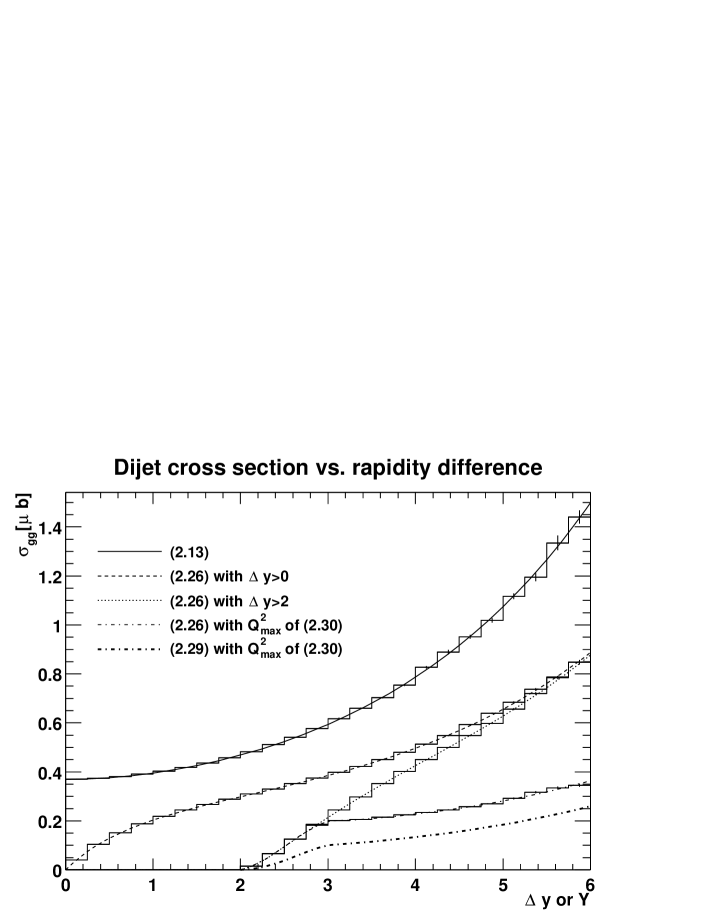
Figure 2: The dependence of the LL BFKL gluon-gluon cross section on $\Delta y$ in the standard Mueller-Navelet calculation (Eq. (2.13)) (upper solid line) and on $Y$ for the D0 setup (Eq. (2.26)). Four curves are shown for the definition of $x$’s applied in the D0 analysis: Dashed line for the requirement $\Delta y>0$, dotted line for $\Delta y>2$, dash-dotted for $Q^{2}_{\rm max}$ of Eq. (2.30) and finally the lower, fat dash-dotted line for the asymptotic behaviour (Eq. (2.29)) using $Q^{2}_{\rm max}$ of Eq. (2.30). The histograms are filled using the MC.

3 Dijet production and energy-momentum conservation

Besides the effects described in the previous section, there are other facts that need to be considered when aiming at comparing experimental data to BFKL predictions, some of general nature and some specific to the experimental set-up of Ref. [18]. We will comment on the latter in the next section. As far as the former are concerned, we remind the reader of the following facts. $(i)$ The LL BFKL resummation is performed at fixed coupling constant, and thus any variation in the scale at which $\alpha_{s}$ is evaluated appears in the next-to-leading-logarithmic (NLL) terms. $(ii)$ Because of the strong rapidity ordering, any two-parton invariant mass is large. Thus there are no collinear divergences in the LL BFKL resummation; jets are determined only at LO and accordingly have a trivial structure. $(iii)$ Energy and longitudinal momentum are not conserved, and since the momentum fractions $x$ of the incoming partons are reconstructed from the kinematic variables of the outgoing partons, the BFKL theory can severely underestimate the exact value of the $x$’s, and thus grossly overestimate the parton luminosities. In fact, if $n+2$ partons are produced, energy-momentum conservation gives

$$x_{a} = \frac{e^{y_{a}}}{\sqrt{S}}\left(\mbox{$k_{a\perp}$}\,+\,\mbox{$k_{b\perp}$}e^{-\Delta y}\,+\,\sum_{i=1}^{n}k_{i\perp}e^{y_{i}-y_{a}}\right)\,,$$

$$x_{b} = \frac{e^{-y_{b}}}{\sqrt{S}}\left(\mbox{$k_{b\perp}$}\,+\,\mbox{$k_{a\perp}$}e^{-\Delta y}\,+\,\sum_{i=1}^{n}k_{i\perp}e^{-y_{i}+y_{b}}\right)\,.$$ (3.1)

The momentum fractions (2.3) in the high-energy limit are recovered by imposing the strong rapidity ordering (2.1). However, the requirement $x_{a},x_{b}\leq 1$ effectively imposes an upper limit on the transverse momentum ($\vec{k}_{i\perp}$) integrals. This effect is completely analogous to that we have considered in sections 2.2 and 2.3.

In an attempt to go beyond the analytic leading-logarithm BFKL results, a Monte Carlo approach has been adopted [25, 10, 26]. If we transform the relevant Green’s function to moment space via

$$f(\vec{q}_{a\perp},\vec{q}_{b\perp},\Delta y)\ =\ \int{d\omega\over 2\pi i}\,e^{\omega\Delta y}\,f_{\omega}(\vec{q}_{a\perp},\vec{q}_{b\perp})\,,$$ (3.2)

(by averaging $f$ over azimuthal angles one obtains the quantity $\bar{f}$ introduced in Eq. (2.5)) we can write the BFKL equation as

$$\omega\,f_{\omega}(\vec{q}_{a\perp},\vec{q}_{b\perp})\,={1\over 2}\,\delta(\vec{q}_{a\perp}-\vec{q}_{b\perp})\,+\,{\bar{\alpha}_{s}\over\pi}\int{d^{2}\vec{k}_{\perp}\over k_{\perp}^{2}}\,K(\vec{q}_{a\perp},\vec{q}_{b\perp},\vec{k}_{\perp})\,,$$ (3.3)

where the kernel $K$ is given by

$$K(\vec{q}_{a\perp},\vec{q}_{b\perp},\vec{k}_{\perp})=f_{\omega}(\vec{q}_{a\perp}+\vec{k}_{\perp},\vec{q}_{b\perp})-{q_{a\perp}^{2}\over k_{\perp}^{2}+(\vec{q}_{a\perp}+\vec{k}_{\perp})^{2}}\,f_{\omega}(\vec{q}_{a\perp},\vec{q}_{b\perp})\,.$$ (3.4)

The first term in the kernel accounts for the emission of a real gluon of transverse momentum $\vec{k}_{\perp}$ and the second term accounts for the virtual radiative corrections. By solving the BFKL equation (3.3) by iteration, which amounts to ‘unfolding’ the summation over the intermediate radiated gluons and making their contributions explicit, it is possible to include the effects of both the running coupling and the overall kinematic constraints. It is also straightforward to implement the resulting iterated solution in an event generator.

The first step in this procedure is to separate the $\vec{k}_{\perp}$ integral in (3.3) into ‘resolved’ and ‘unresolved’ contributions, according to whether they lie above or below a small transverse energy scale $\mu$. The scale $\mu$ is assumed to be small compared to the other relevant scales in the problem (the minimum transverse momentum $E_{\perp}$ for example). The virtual and unresolved contributions are then combined into a single, finite integral. The BFKL equation becomes

$$\omega\,f_{\omega}(\vec{q}_{a\perp},\vec{q}_{b\perp}) = {1\over 2}\,\delta(\vec{q}_{a\perp}-\vec{q}_{b\perp})\,+\,{\bar{\alpha}_{s}\over\pi}\int_{k_{\perp}^{2}>\mu^{2}}{d^{2}\vec{k}_{\perp}\over k_{\perp}^{2}}\,f_{\omega}(\vec{q}_{a\perp}+\vec{k}_{\perp},\vec{q}_{b\perp})$$ (3.5)

$$+ {\bar{\alpha}_{s}\over\pi}\int{d^{2}\vec{k}_{\perp}\over k_{\perp}^{2}}\left[f_{\omega}(\vec{q}_{a\perp}+\vec{k}_{\perp},\vec{q}_{b\perp})\,\theta(\mu^{2}-k_{\perp}^{2})\,-\,{q_{a\perp}^{2}\,f_{\omega}(\vec{q}_{a\perp},\vec{q}_{b\perp})\over k_{\perp}^{2}+(\vec{q}_{a\perp}+\vec{k}_{\perp})^{2}}\right].$$

The combined unresolved/virtual integral can be simplified by noting that since $k_{\perp}^{2}\ll q_{a\perp}^{2},q_{b\perp}^{2}$ by construction, the $\vec{k}_{\perp}$ term in the argument of $f_{\omega}$ can be neglected, giving

$$(\omega-\omega_{0})\,f_{\omega}(\vec{q}_{a\perp},\vec{q}_{b\perp})\,=\,{1\over 2}\,\delta(\vec{q}_{a\perp}-\vec{q}_{b\perp})\,+\,{\bar{\alpha}_{s}\over\pi}\int_{k_{\perp}^{2}>\mu^{2}}{d^{2}\vec{k}_{\perp}\over k_{\perp}^{2}}\,f_{\omega}(\vec{q}_{a\perp}+\vec{k}_{\perp},\vec{q}_{b\perp})\\ \,,$$

where

$$\omega_{0}={\bar{\alpha}_{s}\over\pi}\int{d^{2}\vec{k}_{\perp}\over k_{\perp}^{2}}\left[\theta(\mu^{2}-k_{\perp}^{2})\,-\,{q_{a\perp}^{2}\over\vec{k}_{\perp}^{2}+(\vec{q}_{a\perp}+\vec{k}_{\perp})^{2}}\right]\simeq{\bar{\alpha}_{s}}\,\ln\left({\mu^{2}\over q_{a\perp}^{2}}\right)\,.$$ (3.6)

The virtual and unresolved contributions are now contained in $\omega_{0}$ and we are left with an integral over resolved real gluons. We can now solve (3) iteratively, and performing the inverse transform we have

$$f(\vec{q}_{a\perp},\vec{q}_{b\perp},\Delta y)\,=\,\sum_{n=0}^{\infty}f^{(n)}(\vec{q}_{a\perp},\vec{q}_{b\perp},\Delta y)\;.$$ (3.7)

where

$$f^{(0)}(\vec{q}_{a\perp},\vec{q}_{b\perp},\Delta y) = \left[\frac{\mu^{2}}{q_{a\perp}^{2}}\right]^{\bar{\alpha}_{s}\Delta y}\,\,\frac{1}{2}\,\delta(\vec{q}_{a\perp}-\vec{q}_{b\perp})\,,$$

$$f^{(n\geq 1)}(\vec{q}_{a\perp},\vec{q}_{b\perp},\Delta y) = \left[\frac{\mu^{2}}{q_{a\perp}^{2}}\right]^{\bar{\alpha}_{s}\Delta y}\,\left\{\prod_{i=1}^{n}\int d^{2}\vec{k}_{i\perp}\,dy_{i}\,{\cal F}_{i}\right\}\,\frac{1}{2}\,\delta(\vec{q}_{a\perp}-\vec{q}_{b\perp}-\sum_{i=1}^{n}\vec{k}_{i\perp})\,,$$

$${\cal F}_{i} = \frac{\bar{\alpha}_{s}}{\pi k_{i\perp}^{2}}\,\theta(k_{i\perp}^{2}-\mu^{2})\,\theta(y_{i-1}-y_{i})\,\left[{(\vec{q}_{a\perp}+\sum_{j=1}^{i-1}\vec{k}_{j\perp})^{2}\over(\vec{q}_{a\perp}+\sum_{j=1}^{i}\vec{k}_{j\perp})^{2}}\right]^{\bar{\alpha}_{s}y_{i}}\,.$$ (3.8)

Thus the solution to the BFKL equation is recast in terms of phase space integrals for resolved gluon emissions, with form factors representing the net effect of unresolved and virtual emissions. In this way, each $f^{(n)}$ depends on the resolution parameter $\mu$, whereas the full sum $f$ does not. Changing $\mu$ simply shifts parts of the cross section from one $f^{(n)}$ to another.

Unlike in the case of DGLAP evolution, there is no strong ordering of the transverse momenta $k_{i\perp}$. Strictly speaking, the derivation given above only applies for fixed coupling because we have left $\alpha_{s}$ outside the integrals. The modifications necessary to account for a running coupling $\alpha_{s}(k_{i\perp}^{2})$ are straightforward [10].

The expression for $f$ in Eqs. (3.7) and (3.8) is amenable to numerical integration which can be implemented in the form of a Monte Carlo event generator [25, 10, 26]. In this way we can trivially impose further cuts and combine the subprocess cross section with parton densities. Having made explicit the BFKL gluon emission phase space, overall energy and momentum conservation is imposed by using the momentum fraction definitions in Eq. (3.1). We can also run the Monte Carlo in ‘LL mode’, i.e. with fixed $\alpha_{s}$ and no additional cuts or parton densities, to check that it does indeed reproduce the analytic results of the previous section, see Fig. 1.

4 Equal transverse momentum cuts: a dangerous choice

We now take a closer look at the set-up specific to the D0 analysis of Ref. [18]. As a preliminary observation, we might say that the values $\Delta y$ probed are quite far from the asymptotic region where Eq. (2.16) is expected to hold, particularly at $\sqrt{S}$ = 630 GeV, where $\Delta y$ is of the order of 2 to 3; unfortunately, here the only solution is to wait for the LHC to come into operation. A more serious, but solvable, problem is the following: dijet rates are quite sensitive to the emission of soft and collinear gluons, in the case in which they are defined by imposing equal cuts on the transverse energies of the two tagged jets. In this sense, a dijet total rate is completely analogous to the azimuthal correlation mentioned above. A detailed discussion on this point is given in Ref. [27], and will not be repeated here. In the current study, we will limit ourselves to illustrating the discussion of Ref. [27] by means of examples relevant to dijet production at the Tevatron. We will do this in two steps. First, in Subsection 4.1, we will study this issue using a fixed-order perturbative computation, showing that dijet cross sections defined with unequal transverse momentum cuts do not have the same problems as those defined with equal cuts. Then, in Subsection 4.2, we will repeat the analysis of Section 2 in the more general case of unequal transverse momentum cuts.

4.1 Dijet cross sections at fixed perturbative order

In this subsection, we consider jet production at fixed perturbative order in QCD. In particular, we use the partonic event generator of Ref. [28], which is accurate to NLO for any one- or two-jet observables. Similarly to what has been done previously for the gluon-gluon cross section, we define a total dijet cross section as follows:

$$\sigma({\cal D},{\cal C})=\sigma(\mbox{$k_{a\perp}$}\!>\!\mbox{$E_{\perp}$},\mbox{$k_{b\perp}$}\!>\!\mbox{$E_{\perp}$}+{\cal D},{\cal C}),$$ (4.1)

where ${\cal C}$ generically indicates a set of cuts to be added to transverse-momentum cuts. As already mentioned, D0 have

$${\cal C}:\;\;\;\;\;\;\left|y_{i}\right|<3,\;\;\Delta y>2,\;\;Q^{2}<1000~{}{\rm GeV}^{2}$$ (4.2)

($i=a,b$), together with some additional cuts on $x_{1}$ and $x_{2}$; furthermore, $\mbox{$E_{\perp}$}=20$ GeV.

The rates defined in Eq. (4.1) are shown in Fig. 3, the left (right) panel presenting the case of $\sqrt{S}=630$ GeV ($\sqrt{S}=1800$ GeV). Each plot consists of three sets of results, corresponding to different choices of ${\cal C}$; for each of these choices, both the NLO results (displayed by the solid, dashed, and dotted curves) and the LO results (displayed by the boxes, diamonds and circles) are given. The solid curves and the boxes are obtained by imposing only the pseudorapidity cuts $\left|y_{i}\right|<3$. The dashed curves and the diamonds correspond to the previous cuts on $y_{i}$ plus the cut $\Delta y>2$. Finally, the dotted curves and the circles are relevant to the cuts given in Eq. (4.2), plus those that define bin number 1 (see Table 1). Notice that the results relevant to bin 1 have been multiplied by a factor of 10 and 50 at $\sqrt{S}=630$ GeV and $\sqrt{S}=1800$ GeV respectively, so that they can be shown together with the other results on the same plot.

Figure 3: Dijet rates, as defined in Eq. (4.1), for various cuts ${\cal C}$. The cases of $\sqrt{S}=630$ GeV (left) and of $\sqrt{S}=1800$ GeV (right) are both considered. Dotted curves and circles have been rescaled by factor of 10 (left) and 50 (right). See the text for details.

From the cross section definition in Eq. (4.1), it is clear that the smaller ${\cal D}$, the larger the phase space available; thus, one naively expects that the smaller ${\cal D}$, the larger the cross section. This is indeed what happens at the LO level, regardless of the cuts ${\cal C}$. On the other hand, the NLO cross section increases when ${\cal D}$ decreases only if ${\cal D}$ is not too close to zero; when ${\cal D}$ approaches zero, $\sigma({\cal D})$ has a local maximum, and then turns over, eventually dropping below the LO result. As discussed in Ref. [27], at ${\cal D}=0$ the NLO result is finite (i.e., does not diverge), but the slope $d\sigma/d{\cal D}$ is infinite. Fig. 3 thus clearly shows that at ${\cal D}=0$ (which corresponds to the definition adopted in the experimental analysis) the cross section is affected by large logarithms, that can spoil the analysis performed in terms of BFKL dynamics, exactly as in the case of the azimuthal decorrelation.

	NLO			Born
	${\cal D}=0$	${\cal D}=2$	${\cal D}=4$	${\cal D}=0$	${\cal D}=2$	${\cal D}=4$
bin 1	-0.12(6)	1.55(4)	2.62(7)	1.681(3)	2.340(7)	4.16(3)
bin 2	-0.16(4)	1.14(3)	1.46(4)	1.265(3)	1.417(4)	1.739(8)
bin 3	-0.16(5)	0.92(3)	1.13(4)	1.074(3)	1.098(5)	1.138(6)
bin 4	-0.19(6)	0.92(4)	1.15(5)	1.036(4)	1.045(6)	1.068(8)
bin 5	-0.35(5)	0.82(3)	1.01(4)	1.026(4)	1.027(6)	1.020(7)
bin 6	-0.45(9)	0.82(7)	1.08(9)	1.015(9)	1.01(1)	1.00(1)

Table 2: Fixed-order predictions for the ratio defined in Eq. (1.1). Numbers in parentheses give the statistical error, which affect the last digit of the results shown. The values of ${\cal D}$ are given in GeV.

Fig. 3 already suggests a possible solution to this problem: simply define a dijet rate by considering different transverse momentum cuts on the two jets (that is, ${\cal D}>0$). From the plots, we can expect that the potentially dangerous logarithms affecting the region ${\cal D}=0$ are not large starting from ${\cal D}$ of the order of 3 or 4 GeV. The figure might also at first sight seem to imply that a similar problem arises in the large ${\cal D}$ region in the case in which the (physically relevant) cuts on $x_{1}$ and $x_{2}$ are imposed (dotted curves and circles). However, it is easy to understand that in such a case the large difference between the NLO and LO results is simply due to phase space: in fact, at LO ${\cal D}\geq 0$ effectively forces both jets to have $k_{\perp}\!>\mbox{$E_{\perp}$}+{\cal D}$; at NLO, this is no longer true.

Let us therefore consider again the ratio of Eq. (1.1), now rewritten to indicate explicitly the cuts adopted:

$$R({\cal D},{\cal C})=\sigma({\cal D},{\cal C};\sqrt{S}=1800~{}{\rm GeV})/\sigma({\cal D},{\cal C};\sqrt{S}=630~{}{\rm GeV})\,,$$ (4.3)

with ${\cal C}$ given in Eq. (4.2), and additional (binning) cuts on $x_{1}$ and $x_{2}$. Our predictions for $R$, both at NLO and LO, are presented in Table 2, where we show the results for all of the bins of Table 1. The entries relevant to ${\cal D}=0$ display a pathological (negative) behaviour at NLO. However, even if they were positive, they could not be considered reliable, since any fixed-order QCD computation (beyond LO) is unable to give a sound prediction in this case. On the other hand, we see that for larger values of ${\cal D}$ the situation improves, in the sense that it reproduces our naive expectation: the ratio should converge towards one, for increasing $\Delta y$ (i.e., larger bin numbers); while for ${\cal D}=2$ GeV the NLO results are still sizeably different from the LO results, in the case of ${\cal D}=4$ GeV the NLO and LO results are statistically compatible (within one standard deviation) for bins 3–6, and they are both approaching one.

Inspection of Fig. 3 and Table 2 tells us that, in order to avoid the presence of large logarithms of non-BFKL nature in the cross section, a value of ${\cal D}=4$ GeV is probably a better choice than ${\cal D}=2$ GeV. Of course, the larger ${\cal D}$, the smaller the cross section, and therefore the fewer the events. In order to give an estimate of the loss of events that one faces when going from ${\cal D}=0$ to larger values, we present in Table 3 our LO predictions for the rate defined in Eq. (4.1), with the cuts of Eq. (4.2) and our six bins. Of course, it is well known that NLO corrections are mandatory in jet physics to get good agreement with data. However, here we just want to have a rough idea of the number of events lost when increasing one of the transverse energy cuts; this number is sensibly predicted by the ratio $\sigma({\cal D})/\sigma({\cal D}=0)$, even if $\sigma$ is only computed at LO. From the table, we see that at ${\cal D}=4$ GeV the number of events decreases, compared to the case ${\cal D}=0$, by a factor slightly larger than two; this factor gets much larger only for the first two bins at $\sqrt{S}=630$ GeV, which are however less relevant from the point of view of BFKL dynamics.

	$\sqrt{S}=1.8$ TeV			$\sqrt{S}=0.63$ TeV
	${\cal D}=0$	${\cal D}=2$	${\cal D}=4$	${\cal D}=0$	${\cal D}=2$	${\cal D}=4$
bin 1	31.01(3)	21.24(3)	14.19(2)	18.46(3)	9.080(2)	3.399(1)
bin 2	22.66(2)	15.52(2)	10.36(2)	17.91(2)	10.98(2)	5.969(2)
bin 3	13.50(2)	9.22(2)	6.16(2)	12.57(2)	8.39(2)	5.41(2)
bin 4	12.11(3)	8.29(2)	5.54(2)	11.69(3)	7.20(2)	5.19(2)
bin 5	7.19(1)	4.90(1)	3.26(1)	7.10(1)	4.78(2)	3.19(1)
bin 6	4.25(2)	2.89(2)	1.92(1)	4.19(2)	2.85(2)	1.92(1)

Table 3: Cross sections in nanobarns as given in Eq. (4.1), at the LO and for two different centre-of-mass energies. Statistical errors are given in parentheses.

4.2 Dijet production in the BFKL theory with an asymmetric cut

We now turn again to the BFKL equation, and study the dependence on the offset ${\cal D}$ introduced in the previous subsection, in essentially the same way as we did in Section 2. We start by integrating the gluon-gluon cross section (2.5) over $\mbox{$k_{a\perp}$}\!>\!\mbox{$E_{\perp}$}$ and $\mbox{$k_{b\perp}$}\!>\!\mbox{$E_{\perp}$}+{\cal D}$ with the upper cut $Q^{2}=\mbox{$k_{a\perp}$}\mbox{$k_{b\perp}$}\!\!<1000$ GeV², and with the $x$’s defined as in the Mueller-Navelet analysis, Eq. (2.11),

$$\hat{\sigma}_{gg}(\mbox{$k_{a\perp}$}\!>\!\mbox{$E_{\perp}$},\mbox{$k_{b\perp}$}\!>\!\mbox{$E_{\perp}$}+{\cal D},\mbox{$k_{a\perp}$}\mbox{$k_{b\perp}$}\!\!<Q^{2}_{\rm max})={\pi C_{A}^{2}\alpha_{s}^{2}\over 2\mbox{$E_{\perp}$}(\mbox{$E_{\perp}$}+{\cal D})}$$

$$\times \Biggl{\{}{\cal F}\left(\Delta y,{\mbox{$E_{\perp}$}\over\mbox{$E_{\perp}$}+{\cal D}}\right)-{\mbox{$E_{\perp}$}(\mbox{$E_{\perp}$}+{\cal D})\over 2Q^{2}_{\rm max}}\left[{\cal G}\left(\Delta y,{\mbox{$E_{\perp}^{2}$}\over Q^{2}_{\rm max}}\right)+{\cal G}\left(\Delta y,{(\mbox{$E_{\perp}$}+{\cal D})^{2}\over Q^{2}_{\rm max}}\right)\right]\Biggr{\}}\,,$$

with ${\cal F}$ and ${\cal G}$ defined in Eq. (2.14) and Eq. (2.18). Repeating the calculation as in Section 2.3, with the $x$’s defined as in Eq. (2.3), yields a cross section of the same form as Eq. (4.2) up to replacing the rapidity interval (2.12) with the constant (2.24), the upper bound $Q^{2}_{\rm max}$ above with Eq. (2.30) and the function ${\cal F}$ (${\cal G}$) with $\tilde{\cal F}$ ($\tilde{\cal G}$), Eq. (2.27) (Eq. (2.28)). At ${\cal D}=0$ we recover Eqs. (2.17) and (2.26) respectively. However, near ${\cal D}=0$ Eq. (4.2) and its analogous one with the tilda functions display the same qualitative behaviour when expanded to NLO as the exact NLO cross section [27]. In order to see this, we take Eq. (4.2) in the limit $Q^{2}_{\rm max}\to\infty$, such that only the first term on the right hand side of Eq. (4.2) survives. We analyse its NLO term by expanding its exponential to ${\cal O}(\alpha_{s})$,

$$\hat{\sigma}_{gg}(\mbox{$k_{a\perp}$}\!>\!\mbox{$E_{\perp}$},\mbox{$k_{b\perp}$}\!>\!\mbox{$E_{\perp}$}+{\cal D})$$

$$= {C_{A}^{2}\alpha_{s}^{2}\over 4\mbox{$E_{\perp}$}(\mbox{$E_{\perp}$}+{\cal D})}\int_{-\infty}^{\infty}d\nu\,{1-2{\bar{\alpha}_{s}}\Delta y\,\left[{\rm Re}\,\psi\left({1/2}+i\nu\right)-\psi(1)\right]\over\nu^{2}+1/4}\,\left(\mbox{$E_{\perp}$}\over\mbox{$E_{\perp}$}+{\cal D}\right)^{2i\nu}+{\cal O}\left((\bar{\alpha}_{s}\Delta y)^{2}\right)\,.$$

The denominator has poles at $\nu=\pm i/2$. For the LO term, the integration over $\nu$ is straightforward. For the NLO term, we use the integral representation of the digamma function,

$$\psi(z)-\psi(1)=\int_{0}^{1}dx\ {1-x^{z-1}\over 1-x}$$ (4.6)

and after performing the integrals over $\nu$ and $x$, we find

$$\hat{\sigma}_{gg}(\mbox{$k_{a\perp}$}\!>\!\mbox{$E_{\perp}$},\mbox{$k_{b\perp}$}\!>\!\mbox{$E_{\perp}$}+{\cal D})$$

$$\phantom{\,}={\pi C_{A}^{2}\alpha_{s}^{2}\over 2}\Biggl{\{}{1\over\mbox{$E_{\perp}^{2}$}}\left[1-{\bar{\alpha}_{s}}\Delta y\,\left({-2\mbox{$E_{\perp}$}{\cal D}-{\cal D}^{2}\over(\mbox{$E_{\perp}$}+{\cal D})^{2}}\ln{-2\mbox{$E_{\perp}$}{\cal D}-{\cal D}^{2}\over\mbox{$E_{\perp}^{2}$}}+2\ln{\mbox{$E_{\perp}$}+{\cal D}\over\mbox{$E_{\perp}$}}\right)\right]\theta(-{\cal D})$$

$$\phantom{\,}+{1\over(\mbox{$E_{\perp}$}+{\cal D})^{2}}\left[1-{\bar{\alpha}_{s}}\Delta y\,\left({2\mbox{$E_{\perp}$}{\cal D}+{\cal D}^{2}\over\mbox{$E_{\perp}^{2}$}}\ln{2\mbox{$E_{\perp}$}{\cal D}+{\cal D}^{2}\over(\mbox{$E_{\perp}$}+{\cal D})^{2}}+2\ln{\mbox{$E_{\perp}$}\over\mbox{$E_{\perp}$}+{\cal D}}\right)\right]\theta({\cal D})\Biggr{\}}$$

$$\phantom{\,}+{\cal O}\left((\bar{\alpha}_{s}\Delta y)^{2}\right)\,.$$

At LO, transverse-momentum conservation forces the cross section to behave like $1/\mbox{$E_{\perp}^{2}$}$ for ${\cal D}<0$ and like $1/(\mbox{$E_{\perp}$}+{\cal D})^{2}$ for ${\cal D}>0$, even though the cuts over the transverse momenta are asymmetric, see Fig. 4. For ${\cal D}=0$, Eq. (4.2) reduces to Eq. (2.15). For $|{\cal D}|\ll\mbox{$E_{\perp}$}$, Eq. (4.2) becomes

$$\hat{\sigma}_{gg}(\mbox{$k_{a\perp}$}\!>\!\mbox{$E_{\perp}$},\mbox{$k_{b\perp}$}\!>\!\mbox{$E_{\perp}$}+{\cal D})\ =\ {\pi C_{A}^{2}\alpha_{s}^{2}\over 2\mbox{$E_{\perp}^{2}$}}\left[1-{\bar{\alpha}_{s}}\Delta y\,{2|{\cal D}|\over\mbox{$E_{\perp}$}}\ln{2|{\cal D}|\over\mbox{$E_{\perp}$}}+{\cal O}({\cal D})\right]+{\cal O}\left((\bar{\alpha}_{s}\Delta y)^{2}\right)\,.$$ (4.8)

The slope of Eq. (4.2) with respect to ${\cal D}$ is negative (positive) for ${\cal D}<0\,(>0)$, and infinite at ${\cal D}=0$, in agreement with Ref. [27]. In addition, by using Eq. (4.8) to evaluate the ratio (1.1) and remembering that asymptotically $\Delta y_{{}_{A}}\to\Delta y_{{}_{B}}+2\ln(1800/630)$, we find that the NLO BFKL ratio also goes to 1 as $\Delta y$ grows, in agreement with Table 2.

In the BFKL Monte Carlo approach, the implementation of asymmetric cuts on the jets is straightforward. For fixed $\alpha_{s}$ and no additional cuts or parton densities, the analytic result of Eq. (4.2) is reproduced, see Fig. 4.

Finally, we can use the BFKL Monte Carlo to calculate the ‘D0’ cross section ratios defined in Eq. (1.1), in the various bins. Table 4 gives the predictions using the Monte Carlo run in two modes:

Naive:

fixed $\alpha_{s}$, no kinematic constraints, parton densities evaluated at Bjorken $x$’s given in Eq. (2.3).

Full:

running $\alpha_{s}$, energy–momentum conservation applied, parton densities evaluated at $x_{a}$, $x_{b}$ values given in Eq. (3.1).

Evidently neither the naive BFKL nor the BFKL MC calculation shows the ‘pathological’ behaviour of the exact NLO calculation at ${\cal D}=0$ (this is already apparent from Fig. 4). Instead the numbers are quite stable against variations in ${\cal D}$. For all ${\cal D}$ the naive BFKL calculation shows an initial decrease in the cross section ratios, before reaching a minimum around bin 4 where the expected rise due to BFKL dynamics sets in. The initial decrease is simply the subasymptotic effect of the $\Delta y>2$ cut on the cross section at $\sqrt{s}=630$ GeV, as discussed in Section 2.3, and consistent with the qualitative behaviour of the Born cross section ratios in Table 2. On the other hand, if the effects from the parton densities did factorize out completely, one would expect an asymptotic (in bin number) ratio of $R=(S_{A}/S_{B})^{\lambda}$ with $\lambda=\frac{\alpha_{s}C_{A}}{\pi}4\ln 2\approx 0.45$  [26]. This gives $R\approx 2.6$ for the D0 values. However, we have already argued that such a rise is not expected in the D0 analysis, mainly because of the rather stringent $Q^{2}$ cut (see Fig. 1 and Fig. 2). Furthermore, the expected rise is also slightly decreased by the cut in $x_{a},x_{b}\leq 1$, and hence on $k_{a\perp}$ and $k_{b\perp}$, introduced by the parton densities. The full BFKL MC calculation ratios also show an initial decrease to a minimum around bin 4. However now the ratio is below 1 already from bin 3 onwards. Such an effect was already reported and explained in Ref. [26]. It is a kinematic effect due to an effective upper limit on the transverse momentum allowed for each emitted gluon. As the rapidity separation between the dijets is increased towards its maximum allowed value, the BFKL gluon phase space is squeezed from above and the ‘naive’ cross section is heavily suppressed. The higher the collision energy the more dramatic the effect, and hence the ratio $R$ falls below 1.

	Naive BFKL			BFKL MC
	${\cal D}=0$	${\cal D}=2$	${\cal D}=4$	${\cal D}=0$	${\cal D}=2$	${\cal D}=4$
bin 1	2.16(4)	2.56(5)	3.61(8)	1.615(3)	2.013(5)	2.922(8)
bin 2	1.47(4)	1.53(4)	1.73(4)	1.048(2)	1.114(2)	1.289(3)
bin 3	1.22(4)	1.16(4)	1.10(3)	0.866(2)	0.851(2)	0.872(2)
bin 4	1.18(4)	1.12(4)	1.14(4)	0.806(4)	0.783(2)	0.787(2)
bin 5	1.26(6)	1.14(5)	1.11(5)	0.847(2)	0.824(2)	0.820(3)
bin 6	1.31(8)	1.28(7)	1.20(6)	0.863(3)	0.841(3)	0.838(3)

Table 4: BFKL predictions for the ratio defined in Eq. (1.1). Numbers in parentheses give the statistical error, which affect the last digit of the results shown. The values of ${\cal D}$ are given in GeV.

Figure 4: The dependence of the gluon-gluon subprocess cross section on the offset ${\cal D}$, for fixed separation $\Delta y=3$. The resummed prediction Eq. (4.2) is shown as a solid line, with the results of the corresponding BFKL Monte Carlo calculation superimposed. The dash-dotted line is the LO contribution, and the dashed line is the ${\cal O}(\alpha_{s})$ contribution of Eq. (4.2). The parameter values are $\alpha_{s}=0.164$, $\mbox{$E_{\perp}$}=20$ GeV, $Q^{2}_{\rm max}=\infty$.

5 Conclusions

In this paper, we have reconsidered the suggestion by Mueller and Navelet of studying dijet cross sections at large rapidity intervals and for different hadronic centre-of-mass energies, in order to find evidence of BFKL physics. We were motivated by a recent paper by the D0 Collaboration [18], where dijet data have been used to measure the effective BFKL intercept by comparison with the standard analytic asymptotic formulae given by Mueller and Navelet. In fact, we have argued that the definition of the momentum fractions used by D0 and some of the acceptance cuts imposed by D0 spoil the correctness of this procedure, and require a more careful theoretical investigation.

In particular, we are concerned by a difference between D0 and the standard Mueller-Navelet analysis in the reconstruction of the momentum fraction $x$ of the incoming partons, by the presence of an upper bound on the momentum transfer $Q^{2}$, and by the requirement that the two tagged jets have the same minimum transverse energy.

The $Q^{2}$ cut allows, at the experimental level, and together with the binning cuts on $x_{1,2}$, a reduction of the systematic errors, since in the ratio of the cross sections measured at different centre-of-mass energies the dependence on the parton densities cancels to a significant extent. We have shown that, at the level of partonic cross sections, the upper bound on $Q^{2}$ and the $x$’s used in the D0 analysis reduce the Mueller-Navelet cross section by a factor of more than 5. On the other hand, the dependence on such a cut, as well as the dependence on the precise definition of the $x$’s, cancel out when considering the ratio of cross sections obtained at different energies. However, this is only true when the asymptotic forms of the cross sections are considered. Unfortunately, at the energies and rapidity intervals probed at the Tevatron, it appears that the asymptotic expansions do not reproduce accurately enough the exact analytic results; in particular, the quality of the approximations are worse in the case in which an upper cut on $Q^{2}$ is imposed. We are therefore led to conclude that, regardless of the use of cross sections or of rates of cross sections to study BFKL physics, the effect of an upper bound on $Q^{2}$ cannot be ignored.

As far as the cuts on the transverse momenta of the trigger jets are concerned, we have pointed out that in the case in which such cuts are chosen to be equal, the cross sections are plagued with large logarithms of perturbative, non-BFKL origin. In this sense, the total dijet rates are therefore on the same footing as the azimuthal decorrelations. We therefore believe that a much safer choice is to have different cuts on the transverse momenta of the two jets.

References

- [1] A. H. Mueller and H. Navelet, Nucl. Phys. B282 (1987) 727.
- [2] E. A. Kuraev, L. N. Lipatov and V. S. Fadin, Sov. Phys. JETP 44 (1976) 443.
- [3] E. A. Kuraev, L. N. Lipatov and V. S. Fadin, Sov. Phys. JETP 45 (1977) 199.
- [4] I. I. Balitsky and L. N. Lipatov, Sov. J. Nucl. Phys. 28 (1978) 822.
- [5] V. Del Duca and C. R. Schmidt, Phys. Rev. D49 (1994) 4510 [hep-ph/9311290].
- [6] W. J. Stirling, Nucl. Phys. B423 (1994) 56 [hep-ph/9401266].
- [7] V. Del Duca and C. R. Schmidt, hep-ph/9410341. Talk at the 6th Rencontres de Blois, France, 1994.
- [8] V. Del Duca and C. R. Schmidt, Nucl. Phys. Proc. Suppl. 39BC (1995) 137 [hep-ph/9408239].
- [9] V. Del Duca and C. R. Schmidt, Phys. Rev. D51 (1995) 2150 [hep-ph/9407359].
- [10] L. H. Orr and W. J. Stirling, Phys. Rev. D56 (1997) 5875 [hep-ph/9706529].
- [11] S. Abachi et al. [D0 Collaboration], Phys. Rev. Lett. 77 (1996) 595 [hep-ex/9603010].
- [12] W. T. Giele, E. W. Glover and D. A. Kosower, Nucl. Phys. B403 (1993) 633 [hep-ph/9302225].
- [13] W. T. Giele, E. W. Glover and D. A. Kosower, Phys. Rev. Lett. 73 (1994) 2019 [hep-ph/9403347].
- [14] G. Marchesini and B. R. Webber, Nucl. Phys. B310 (1988) 461.
- [15] I. G. Knowles, Nucl. Phys. B310 (1988) 571.
- [16] G. Marchesini, B. R. Webber, G. Abbiendi, I. G. Knowles, M. H. Seymour and L. Stanco, Comput. Phys. Commun. 67 (1992) 465.
- [17] Y. L. Dokshitzer, hep-ph/9801372. Plenary talk at the International Europhysics Conference on High-Energy Physics (HEP 97), Jerusalem, Israel, 1997.
- [18] B. Abbott et al. [D0 Collaboration], Phys. Rev. Lett. 84 (2000) 5722 [hep-ex/9912032].
- [19] S. D. Ellis, Z. Kunszt and D. E. Soper, Phys. Rev. Lett. 69 (1992) 3615 [hep-ph/9208249].
- [20] F. Abe et al. [CDF Collaboration], Phys. Rev. Lett. 69 (1992) 2896.
- [21] H. Weerts [D0 Collaboration], FERMILAB-CONF-94-035-E Presented at 9th Topical Workshop on Proton - Anti-proton Collider Physics, Tsukuba, Japan, 18-22 Oct 1993.
- [22] F. Abe et al. [CDF Collaboration], Phys. Rev. Lett. 77 (1996) 5336 [hep-ex/9609011].
- [23] B. Abbott et al. [D0 Collaboration], Phys. Rev. Lett. 80 (1998) 666 [hep-ex/9707016].
- [24] B. L. Combridge and C. J. Maxwell, Nucl. Phys. B239 (1984) 429.
- [25] C. R. Schmidt, Phys. Rev. Lett. 78 (1997) 4531 [hep-ph/9612454].
- [26] L. H. Orr and W. J. Stirling, Phys. Lett. B429 (1998) 135 [hep-ph/9801304].
- [27] S. Frixione and G. Ridolfi, Nucl. Phys. B507 (1997) 315 [hep-ph/9707345].
- [28] S. Frixione, Nucl. Phys. B507 (1997) 295 [hep-ph/9706545].