Effective Average Action
in Statistical Physics and Quantum Field Theory

Abstract

An exact renormalization group equation describes the dependence of the free energy on an infrared cutoff for the quantum or thermal fluctuations. It interpolates between the microphysical laws and the complex macroscopic phenomena. We present a simple unified description of critical phenomena for $O(N)$-symmetric scalar models in two, three or four dimensions, including essential scaling for the Kosterlitz-Thouless transition.

1 Introduction

Particle physics and statistical physics share a common theoretical challenge. For given “microphysical laws” observable “macrophysical” quantities at much larger characteristic length scales have to be computed. This concerns, for example, the computation of the hadron spectrum from perturbative QCD or the thermodynamic equation state for a liquid of helium from the atomic interactions. The difficulties arise from the importance of fluctuations. More technically, the “transition to macrophysics” requires the solution of a complicated functional integral. Beyond the identical conceptual setting of particle and statistical physics there is also quantitative agreement for certain questions. The critical exponents at the endpoint of the critical line of the electroweak phase transition (the onset of crossover for the critical mass of the Higgs scalar) are believed to be precisely the same as for the liquid-gas transition near the critical pressure. This reflects universality.

Exact renormalization group equations aim for a piecewise solution of the fluctuation problem. They describe the scale dependence of some type of “effective action”. In this context an effective action is a functional of fields from which the physical properties at a given length or momentum scale can be computed. The exact equations can be derived as formal identities from the functional integral which defines the theory. They are cast in the form of functional differential equations. Different versions of exact renormalization group equations have already a long history [1]–[7]. The investigation of the generic features of their solutions has led to a deep insight into the nature of renormalizability. In particle physics, the discussion of perturbative solutions has led to a new proof of perturbative renormalizability of the $\phi^{4}$-theory [6]. Nevertheless, the application of exact renormalization group methods to non-perturbative situations has been hindered for a long time by the complexity of functional differential equations. Some type of expansion is needed if one wants to exploit the exactness of the functional differential equation in practice – otherwise any reasonable guess of a realistic renormalization group equation does as well.

Since exact solutions to functional differential equations seem only possible for some limiting cases, it is crucial to find a formulation which permits non-perturbative approximations. These proceed by a truncation of the most general form of the effective action and therefore need a qualitative understanding of its properties. The formulation of an exact renormalization group equation based on the effective average action [8, 9] has been proven successful in this respect. It is the basis of the non-perturbative flow equations which we discuss in this review. The effective average action is the generating functional of one-particle irreducible correlation functions in the presence of an infrared cutoff scale $k$. Only fluctuations with momenta larger than $k$ are included in its computation. For $k\to 0$ all fluctuations are included and one obtains the usual effective action from which appropriate masses and vertices can be read off directly. The $k$ dependence is described by an exact renormalization group equation that closely resembles a renormalization group improved one-loop equation [9]. In fact, the transition from classical propagators and vertices to effective propagators and vertices transforms the one-loop expression into an exact result. This close connection to perturbation theory for which we have intuitive understanding is an important key for devising non-perturbative approximations. Furthermore, the one-loop expression is manifestly infrared and ultraviolet finite and can be used directly in arbitrary number of dimensions, even in the presence of massless modes.

The aim of this review is to show that this version of flow equations can be used in practice for the transition from microphysics to macrophysics, even in the presence of strong couplings and a large correlation length. It is largely based on a more extensive report by J. Berges, N. Tetradis, and the author [10]. (We refer to this report as well as to [11] for a more extensive list of references.) We derive the exact renormalization group equation and various non-perturbative truncations in section 2. In section 3 we discuss the solutions to the flow equation in more detail for $O(N)$-symmetric scalar models. We derive the scaling form of the flow equation for the effective potential and compute critical exponents for second-order phase transitions in three dimensions. Finally we discuss essential scaling for the Kosterlitz-Thouless phase transition for two-dimensional models with a continuous Abelian symmetry.

Several results in statistical and particle physics have been obtained first with the method presented here. This includes the universal critical equation of state for spontaneous breaking of a continuous symmetry in Heisenberg models [12], the universal critical equation of state for first-order phase transitions in matrix models [13], the non-universal critical amplitudes with an explicit connection of the critical behavior to microphysics $(CO_{2})$ [14], a quantitatively reliable estimate of the rate of spontaneous nucleation [15, 16], a classification of all possible fixed points for (one component) scalar theories in two and three dimensions in case of a weak momentum dependence of the interactions [17], the second-order phase transition in the high temperature $\phi^{4}$ quantum field theory [18], the phase diagram for the Abelian Higgs model for $N$ charged scalar fields [19, 20]. In particle physics it has led to the prediction that the electroweak interactions become strong at high temperature, with the suggestion that the standard model may show a crossover instead of a phase transition [21, 22]. In strong interaction physics the interpolation between the low temperature chiral perturbation theory results and the high temperature critical behavior for two light quarks has been established in an effective model [23]. All these results are in the non-perturbative domain. In addition, the approach has been tested successfully through a comparison with known high precision results on critical exponents and universal critical amplitude ratios and effective couplings.

Our main conclusion can be drawn already at this place: the method works in practice. If needed and with sufficient effort precise results can be obtained in many non-perturbative situations. New phenomena become accessible to a reliable analytical treatment.

2 Non-Perturbative flow equation

2.1 Average action

We will concentrate on a flow equation which describes the scale dependence of the effective average action $\Gamma_{k}$ [9]. The latter is based on the quantum field theoretical concept of the effective action $\Gamma$, i.e. the generating functional of the Euclidean one-particle irreducible ($1PI$) correlation functions or proper vertices. For the vacuum or ground state this functional is obtained after “integrating out” the quantum fluctuations. The masses of the excitations, scattering amplitudes and cross sections follow directly from an analytic continuation of the 1PI correlation functions in a standard way. Furthermore, the field equations derived from the effective action are exact as all quantum effects are included. In thermal and chemical equilibrium $\Gamma$ includes in addition the thermal fluctuations and depends on the temperature $T$ and chemical potential $\mu$. In statistical physics $\Gamma$ is related to the free energy as a functional of some space-dependent order parameter $\phi(x)$. For vanishing external fields the equilibrium state is given by the minimum of $\Gamma$. More generally, in the presence of (spatially varying) external fields or sources the equilibrium state obeys

$$\frac{\delta\Gamma}{\delta\phi(x)}=J(x),$$ (2.1)

and the precise relation to the thermodynamic potentials like the free energy $F$ reads

$$F=T\Gamma_{eq}+\mu\overline{N}-T\int dx\,\phi_{eq}(x)J(x).$$ (2.2)

Here $\phi_{eq}(x)$ solves (2.1), $\Gamma_{eq}=\Gamma[\phi_{eq}]$, and $\overline{N}$ is the conserved quantity to which the chemical potential is associated. For homogeneous $J=j/T$ the equilibrium value of the order parameter $\phi$ is often also homogeneous. In this case the energy density $\epsilon$, entropy density $s$, “particle density” $n$ and pressure $p$ can be simply expressed in terms of the effective potential $U(\phi)=T\Gamma/V$, namely

$$\epsilon=U-T\frac{\partial U}{\partial T}-\mu\frac{\partial U}{\partial\mu}\ ,\ s=-\frac{\partial U}{\partial T}+\frac{j\phi}{T},$$

$$n=-\frac{\partial U}{\partial\mu}\ ,\ p=-U=-T\Gamma/V.$$ (2.3)

Here $U$ has to be evaluated for the solution of $\partial U/\partial\phi=j$, $n=\overline{N}/V$ and $V$ is the total volume of (three-dimensional) space. Evaluating $U$ for arbitrary $\phi$ yields the equation of state in the presence of homogeneous magnetic fields or other appropriate sources.

More formally, the effective action $\Gamma$ follows from a Legendre transform of the logarithm of the partition function in the presence of external sources or fields (see below). Knowledge of $\Gamma$ is in a sense equivalent to the “solution” of a theory. Therefore $\Gamma$ is the macroscopic quantity on which we will concentrate. In particular, the effective potential $U$ contains already a large part of the macroscopic information relevant for homogeneous states. We emphasize that the concept of the effective potential is valid universally for classical statistics and quantum statistics, or quantum field theory in thermal equilibrium or the vacuum.

The average action $\Gamma_{k}$ is a simple generalization of the effective action, with the distinction that only fluctuations with momenta $q^{2}\gtrsim k^{2}$ are included. This is achieved by implementing an infrared (IR) cutoff $\sim k$ in the functional integral that defines the effective action $\Gamma$. In the language of statistical physics, $\Gamma_{k}$ is a type of coarse-grained free energy with a coarse graining length scale $\sim k^{-1}$. As long as $k$ remains large enough, the possible complicated effects of coherent long-distance fluctuations play no role and $\Gamma_{k}$ is close to the microscopic action. Lowering $k$ results in a successive inclusion of fluctuations with momenta $q^{2}\gtrsim k^{2}$ and therefore permits to explore the theory on larger and larger length scales. The average action $\Gamma_{k}$ can be viewed as the effective action for averages of fields over a volume with size $k^{-d}$ [8] and is similar in spirit to the action for block–spins on the sites of a coarse lattice.

By definition, the average action equals the standard effective action for $k=0$, i.e. $\Gamma_{0}=\Gamma$, as the IR cutoff is absent in this limit and all fluctuations are included. On the other hand, in a model with a physical ultraviolet (UV) cutoff $\Lambda$ we can associate $\Gamma_{\Lambda}$ with the microscopic or classical action $S$. No fluctuations with momenta below $\Lambda$ are effectively included if the IR cutoff equals the UV cutoff. Thus the average action $\Gamma_{k}$ has the important property that it interpolates between the classical action $S$ and the effective action $\Gamma$ as $k$ is lowered from the ultraviolet cutoff $\Lambda$ to zero:

$$\Gamma_{\Lambda}\approx S\ ,\,\,\lim\limits_{k\to 0}\Gamma_{k}=\Gamma.$$ (2.4)

The ability to follow the evolution to $k\rightarrow 0$ is equivalent to the ability to solve the theory. Most importantly, the dependence of the average action on the scale $k$ is described by an exact non-perturbative flow equation presented in the next subsection.

Let us consider the construction of $\Gamma_{k}$ for a simple model with real scalar fields $\chi_{a}$, $a=1\ldots N$, in $d$ Euclidean dimensions with classical action $S$. We start with the path integral representation of the generating functional for the connected correlation functions in the presence of an IR cutoff. It is given by the logarithm of the (grand) canonical partition function in the presence of inhomogeneous external fields or sources $J_{a}$

$$W_{k}[J]=\ln Z[J]=\ln\int D\chi\exp\left(-S[\chi]-\Delta S_{k}[\chi]+\int d^{d}xJ_{a}(x)\chi^{a}(x)\right)\;.$$ (2.5)

In classical statistical physics $S$ is related to the Hamiltonean $H$ by $S=H/T$, so that $e^{-S}$ is the usual Boltzmann factor. The functional integration $\int D\chi$ stands for the sum over all microscopic states. In turn, the field $\chi_{a}(x)$ can represent a large variety of physical objects like a (mass-) density field $(N=1)$, a local magnetisation $(N=3)$ or a charged order parameter $(N=2)$. The only modification compared to the construction of the standard effective action is the addition of an IR cutoff term $\Delta S_{k}[\chi]$ which is quadratic in the fields and reads in momentum space $(\chi_{a}(-q)\equiv\chi_{a}^{*}(q))$

$$\Delta S_{k}[\chi]=\frac{1}{2}\int\frac{d^{d}q}{(2\pi)^{d}}R_{k}(q)\chi_{a}(-q)\chi^{a}(q).$$ (2.6)

Here the IR cutoff function $R_{k}$ is required to vanish for $k\to 0$ and to diverge for $k\to\infty$ (or $k\to\Lambda)$ and fixed $q^{2}$. This can be achieved, for example, by the exponential form

$$R_{k}(q)=\frac{Z_{k}q^{2}}{\displaystyle{e^{q^{2}/k^{2}}-1}}$$ (2.7)

where the wave function renormalization constant $Z_{k}$ will be defined later. For fluctuations with small momenta $q^{2}\ll k^{2}$ this cutoff behaves as $R_{k}(q)\sim k^{2}$ and allows for a simple interpretation: Since $\Delta S_{k}[\chi]$ is quadratic in the fields, all Fourier modes of $\chi$ with momenta smaller than $k$ acquire an effective mass $\sim k$. This additional mass term acts as an effective IR cutoff for the low momentum modes. In contrast, for $q^{2}\gg k^{2}$ the function $R_{k}(q)$ vanishes so that the functional integration of the high momentum modes is not disturbed. The term $\Delta S_{k}[\chi]$ added to the classical action is the main ingredient for the construction of an effective action that includes all fluctuations with momenta $q^{2}\gtrsim k^{2}$, whereas fluctuations with $q^{2}\lesssim k^{2}$ are suppressed.

The expectation value of $\chi$, i.e. the macroscopic field $\phi$, in the presence of $\Delta S_{k}[\chi]$ and $J$ reads

$$\phi^{a}(x)\equiv\langle\chi^{a}(x)\rangle=\frac{\delta W_{k}[J]}{\delta J_{a}(x)}.$$ (2.8)

We note that the relation between $\phi$ and $J$ is $k$–dependent, $\phi=\phi_{k}[J]$ and therefore $J=J_{k}[\phi]$. In terms of $W_{k}$ the average action is defined via a modified Legendre transform

$$\Gamma_{k}[\phi]=-W_{k}[J]+\int d^{d}xJ_{a}(x)\phi^{a}(x)-\Delta S_{k}[\phi],$$ (2.9)

where we have subtracted the term $\Delta S_{k}[\phi]$ in the rhs. This subtraction of the IR cutoff term as a function of the macroscopic field $\phi$ is crucial for the definition of a reasonable coarse-grained free energy with the property $\Gamma_{\Lambda}\approx S$. It guarantees that the only difference between $\Gamma_{k}$ and $\Gamma$ is the effective infrared cutoff in the fluctuations. Furthermore, it has the consequence that $\Gamma_{k}$ does not need to be convex, whereas a pure Legendre transform is always convex by definition. The coarse-grained free energy has to become convex [24, 25] only for $k\rightarrow 0$. These considerations are important for an understanding of spontaneous symmetry breaking and, in particular, for a discussion of nucleation in a first-order phase transition.

In order to establish the property $\Gamma_{\Lambda}\approx S$ we consider an integral equation for $\Gamma_{k}$ that is equivalent to (2.9). In an obvious matrix notation, where $J\chi\equiv\int d^{d}xJ_{a}(x)\chi^{a}(x)=\int\frac{d^{d}p}{(2\pi)^{d}}J_{a}(-p)\chi_{a}(p)$ and $R_{k,ab}(q,q^{\prime})=R_{k}(q)\delta_{ab}(2\pi)^{d}\delta(q-q^{\prime})$, we represent (2.5) as

$$\exp\Big{(}W_{k}[J]\Big{)}=\int D\chi\exp\left(-S[\chi]+J\chi-\frac{1}{2}\chi\,R_{k}\chi\right)\;.$$ (2.10)

As usual, we can invert the Legendre transform (2.9) to express

$$J=\frac{\delta\Gamma_{k}}{\delta\phi}+\phi\,R_{k}.$$ (2.11)

It is now straightforward to insert the definition (2.9) into (2.10). After a variable substitution $\chi^{\prime}=\chi-\phi$ one obtains the functional integral representation of $\Gamma_{k}$

$$\exp(-\Gamma_{k}[\phi])=\displaystyle{\int D\chi^{\prime}\exp\left(-S[\phi+\chi^{\prime}]+\frac{\delta\Gamma_{k}}{\delta\phi}\chi^{\prime}-\frac{1}{2}\chi^{\prime}\,R_{k}\,\chi^{\prime}\right)}\;.$$ (2.12)

This expression resembles closely the background field formalism for the effective action which is modified only by the term $\sim R_{k}$. For $k\to\infty$ the cutoff function $R_{k}$ diverges and the term $\exp(-\chi^{\prime}R_{k}\chi^{\prime}/2)$ behaves as a delta functional $\sim\delta[\chi^{\prime}]$, thus leading to the property $\Gamma_{k}\to S$ in this limit. For a model with a sharp UV cutoff $\Lambda$ it is easy to enforce the identity $\Gamma_{\Lambda}=S$ by choosing a cutoff function $R_{k}$ which diverges for $k\to\Lambda$, like $R_{k}\sim q^{2}(e^{q^{2}/k^{2}}-e^{q^{2}/\Lambda^{2}})^{-1}$. We note, however, that the property $\Gamma_{\Lambda}=S$ is not essential, as the short distance laws may be parameterized by $\Gamma_{\Lambda}$ as well as by $S$. For momentum scales much smaller than $\Lambda$ universality implies that the precise form of $\Gamma_{\Lambda}$ is irrelevant, up to the values of a few relevant renormalized couplings. Furthermore, the microscopic action may be formulated on a lattice instead of continuous space and can involve even variables different from $\chi_{a}(x)$. In this case one can still compute $\Gamma_{\Lambda}$ in a first step by evaluating the functional integral (2.12) approximately. Often a saddle point expansion will do, since no long-range fluctuations are involved in the transition from $S$ to $\Gamma_{\Lambda}$. In this report we will assume that the first step of the computation of $\Gamma_{\Lambda}$ is done and consider $\Gamma_{\Lambda}$ as the appropriate parametrization of the microscopic physical laws. Our aim is the computation of the effective action $\Gamma$ from $\Gamma_{\Lambda}$ – this step may be called “transition to complexity” and involves fluctuations on all scales. We emphasize that for large $\Lambda$ the average action $\Gamma_{\Lambda}$ can serve as a formulation of the microscopic laws also for situations where no physical cutoff is present, or where a momentum UV cutoff may even be in conflict with the symmetries, like the important case of gauge symmetries.

A few properties of the effective average action are worth mentioning:

1. All symmetries of the model which are respected by the IR cutoff $\Delta S_{k}$ are automatically symmetries of $\Gamma_{k}$. In particular this concerns translation and rotation invariance. As a result the approach is not plagued by many of the problems encountered by a formulation of the block-spin action on a lattice. Nevertheless, our method is not restricted to continuous space. For a cubic lattice with lattice distance $a$ the propagator only obeys the restricted lattice translation and rotation symmetries, e.g. a next neighbor interaction leads in momentum space to

   $$S=\frac{2}{a^{2}}\int\frac{d^{d}q}{(2\pi)^{d}}\sum\limits_{\mu}\left(1-\cos aq_{\mu}\right)\chi^{*}(q)\chi(q)+\ldots$$ (2.13)

   The momentum cutoff $|q_{\mu}|\leq\Lambda$, $\Lambda=\pi/a$ also reflects the lattice symmetry. A rotation and translation symmetric cutoff $R_{k}$ which only depends on $q^{2}$ obeys automatically all possible lattice symmetries. The only change compared to continuous space will be the reduced symmetry of $\Gamma_{k}$.

2. In consequence, $\Gamma_{k}$ can be expanded in terms of invariants with respect to the symmetries with couplings depending on $k$. For the example of a scalar $O(N)$-model in continuous space one may use a derivative expansion ($\rho=\phi^{a}\phi_{a}/2$)

   $$\Gamma_{k}=\int d^{d}x\left\{U_{k}(\rho)+\frac{1}{2}Z_{\phi,k}(\rho)\partial^{\mu}\phi_{a}\partial_{\mu}\phi^{a}+\ldots\right\}$$ (2.14)

   and expand further in powers of $\rho$

   $$\displaystyle{U_{k}(\rho)} = \displaystyle{\frac{1}{2}\overline{\lambda}_{k}\left(\rho-\rho_{0}(k)\right)^{2}+\frac{1}{6}\overline{\gamma}_{k}\left(\rho-\rho_{0}(k)\right)^{3}+\ldots}\vspace{.2cm}$$

   $$\displaystyle{Z_{\phi,k}(\rho)} = \displaystyle{Z_{\phi,k}(\rho_{0})+Z_{\phi,k}^{\prime}(\rho_{0})\left(\rho-\rho_{0}\right)+\ldots}\;$$ (2.15)

   Here $\rho_{0}$ denotes the ($k$–dependent) minimum of the effective average potential $U_{k}(\rho)$. We see that $\Gamma_{k}$ describes infinitely many running couplings.

3. Up to an overall scale factor, the limit $k\to 0$ of $U_{k}$ corresponds to the effective potential $U=T\Gamma/V$, from which the thermodynamic quantities can be derived for homogeneous situations according to eq. (2.1). The overall scale factor is fixed by dimensional considerations. Whereas the dimension of $U_{k}$ is (mass)^d the dimension of $U$ in eq. (2.1) is (mass)⁴ (for $h\!\!\bar{}\,\,=c=k_{B}=1$). For classical statistics in $d=3$ dimensions one has $U_{k}=\Gamma_{k}/V$ and $U=T\lim_{k\to 0}U_{k}$. For two-dimensional systems an additional factor $\sim$ mass appears, since $U_{k}=\Gamma_{k}/V_{2}=L\Gamma_{k}/V$ implies $U=TL^{-1}\lim_{k\to 0}U_{k}$. Here $L$ is the typical thickness of the two-dimensional layers in a physical system. In the following we will often omit these scale factors.

4. The functional $\tilde{\Gamma}_{k}[\phi]=\Gamma_{k}[\phi]+\Delta S_{k}[\phi]$ is the Legendre transform of $W_{k}$ and therefore convex. This implies that all eigenvalues of the matrix of second functional derivatives $\Gamma^{(2)}+R_{k}$ are positive semi-definite. In particular, one finds for a homogeneous field $\phi_{a}$ and $q^{2}=0$ the simple exact bounds for all $k$ and $\rho$

   $$U_{k}^{\prime}(\rho) \geq -R_{k}(0)\vspace{.2cm}$$

   $$U_{k}^{\prime}(\rho)+2\rho U_{k}^{\prime\prime}(\rho) \geq -R_{k}(0),$$ (2.16)

   where primes denote derivatives with respect to $\rho$. Even though the potential $U(\phi)$ becomes convex for $k\to 0$ it may exhibit a minimum at $\rho_{0}(k)>0$ for all $k>0$. Spontaneous breaking of the $O(N)$-symmetry is characterized by $\lim_{k\to 0}\rho_{0}(k)>0$.

5. The results for physical quantities have to be independent of the choice of the cutoff scheme $R_{k}$. On the other hand, both $\Gamma_{\Lambda}$ and the flow with $k$ are scheme-dependent. The scheme independence of the final results is a good check for approximations [8, 26, 27, 28, 29].

6. There is no problem incorporating chiral fermions, since a chirally invariant cutoff $R_{k}$ can be formulated [30, 31]. Gauge theories can be formulated along similar lines [32, 33, 21], [34]–[40] even though $\Delta S_{k}$ may not be gauge invariant. In this case the usual Ward identities receive corrections for which one can derive closed expressions [32, 36]. These corrections vanish for $k\rightarrow 0$. On the other hand they appear as “counterterms” in $\Gamma_{\Lambda}$ and are crucial for preserving the gauge invariance of physical quantities.

7. Despite a similar spirit and many analogies, there is a conceptual difference to the Wilsonian effective action $S_{\Lambda}^{\rm W}$. The Wilsonian effective action describes a set of different actions (parameterized by $\Lambda$) for one and the same model — the n–point functions are independent of $\Lambda$ and have to be computed from $S_{\Lambda}^{\rm W}$ by further functional integration. In contrast, $\Gamma_{k}$ can be viewed as the effective action for a set of different “models” — for any value of $k$ the effective average action is related to the generating functional of 1PI $n$-point functions for a model with a different action $S_{k}=S+\Delta S_{k}$. The $n$–point functions depend on $k$. The Wilsonian effective action does not generate the 1PI Green functions [42].

2.2 Exact flow equation

The dependence of the average action $\Gamma_{k}$ on the coarse graining scale $k$ is described by an exact non-perturbative flow equation [9, 43, 44, 45]

$$\frac{\partial}{\partial k}\Gamma_{k}[\phi]=\frac{1}{2}\hbox{Tr}\left\{\left[\Gamma_{k}^{(2)}[\phi]+R_{k}\right]^{-1}\frac{\partial}{\partial k}R_{k}\right\}\;.$$ (2.17)

The trace involves an integration over momenta or coordinates as well as a summation over internal indices. In momentum space it reads $\hbox{Tr}=\sum_{a}\int d^{d}q/(2\pi)^{d}$, as appropriate for the unit matrix ${\bf 1}=(2\pi)^{d}\delta(q-q^{\prime})\delta_{ab}$. The exact flow equation describes the scale dependence of $\Gamma_{k}$ in terms of the inverse average propagator $\Gamma_{k}^{(2)}$, given by the second functional derivative of $\Gamma_{k}$ with respect to the field components

$$\left(\Gamma_{k}^{(2)}\right)_{ab}(q,q^{\prime})=\frac{\delta^{2}\Gamma_{k}}{\delta\phi^{a}(-q)\delta\phi^{b}(q^{\prime})}\;.$$ (2.18)

It has a simple graphical expression as a one-loop equation

$\displaystyle{\frac{\partial\Gamma_{k}}{\partial k}\,\,\,\,=\,\,\,\,\frac{1}{2}\,\,\,\,}$

with the full $k$–dependent propagator associated to the propagator line and the dot denoting the insertion $\partial_{k}R_{k}$.

Because of the appearance of the exact propagator $(\Gamma_{k}^{(2)}+R_{k})^{-1}$, eq. (2.17) is a functional differential equation. It is remarkable that the transition from the classical propagator in the presence of the infrared cutoff, $(S^{(2)}+R_{k})^{-1}$, to the full propagator turns the one-loop expression into an exact identity which incorporates effects of arbitrarily high loop order as well as genuinely non-perturbative effects like instantons in QCD.

The exact flow equation (2.17) can be derived in a straightforward way [9]. Let us write

$$\Gamma_{k}[\phi]=\tilde{\Gamma}_{k}[\phi]-\Delta S_{k}[\phi],$$ (2.19)

where, according to (2.9),

$$\tilde{\Gamma}_{k}[\phi]=-W_{k}[J]+\int d^{d}xJ(x)\phi(x)$$ (2.20)

and $J=J_{k}(\phi)$. We consider for simplicity a one–component field and derive first the scale dependence of $\tilde{\Gamma}$:

$$\frac{\partial}{\partial k}\tilde{\Gamma}_{k}[\phi]=-\left(\frac{\partial W_{k}}{\partial k}\right)[J]-\int d^{d}x\frac{\delta W_{k}}{\delta J(x)}\frac{\partial J(x)}{\partial k}+\int d^{d}x\phi(x)\frac{\partial J(x)}{\partial k}\;.$$ (2.21)

With $\phi(x)=\delta W_{k}/\delta J(x)$ the last two terms in (2.21) cancel. The $k$–derivative of $W_{k}$ is obtained from its defining functional integral (2.5). Since only $R_{k}$ depends on $k$ this yields

$$\frac{\partial}{\partial k}\tilde{\Gamma}_{k}[\phi]=\left\langle\frac{\partial}{\partial k}\Delta S_{k}[\chi]\right\rangle=\left\langle\frac{1}{2}\int d^{d}xd^{d}y\chi(x)\frac{\partial}{\partial k}R_{k}(x,y)\chi(y)\right\rangle\;,$$ (2.22)

where $R_{k}(x,y)=R_{k}(x-y)$ is the Fourier transform of $R_{k}(q)$ and

$$\left\langle A[\chi]\right\rangle=Z^{-1}\int D\chi A[\chi]\exp(-S[\chi]-\Delta_{k}S[\chi]+\int d^{d}xJ(x)\chi(x)).$$ (2.23)

Let $G(x,y)=\delta^{2}W_{k}/\delta J(x)\delta J(y)$ denote the connected $2$–point function and decompose

$$\langle\chi(x)\chi(y)\rangle=G(x,y)+\langle\chi(x)\rangle\langle\chi(y)\rangle\equiv G(x,y)+\phi(x)\phi(y)\;.$$ (2.24)

After plugging this decomposition into (2.22), the scale dependence of $\tilde{\Gamma}_{k}$ can be expressed as

$$\frac{\partial}{\partial k}\tilde{\Gamma}_{k}[\phi] = \frac{1}{2}\int d^{d}xd^{d}y\left\{\frac{\partial}{\partial k}R_{k}(x,y)G(y,x)+\phi(x)\frac{\partial}{\partial k}R_{k}(x,y)\phi(y)\right\}\vspace{.2cm}$$ (2.25)

$$\equiv \frac{1}{2}\hbox{Tr}\left\{G\frac{\partial}{\partial k}R_{k}\right\}+\frac{\partial}{\partial k}\Delta S_{k}[\phi]\;.$$

The exact flow equation for the average action $\Gamma_{k}$ follows now through (2.19)

$$\frac{\partial}{\partial k}\Gamma_{k}[\phi]=\frac{1}{2}\hbox{Tr}\left\{G\frac{\partial}{\partial k}R_{k}\right\}=\frac{1}{2}\hbox{Tr}\left\{\left[\Gamma_{k}^{(2)}[\phi]+R_{k}\right]^{-1}\frac{\partial}{\partial k}R_{k}\right\}.$$ (2.26)

For the last equation we have used that $\tilde{\Gamma}_{k}^{(2)}(x,y)\equiv\delta^{2}\tilde{\Gamma}_{k}/\delta\phi(x)\delta\phi(y)=\delta J(x)/\delta\phi(y)$ is the inverse of $G(x,y)\equiv\delta^{2}W_{k}/\delta J(x)\delta J(y)=\delta\phi(x)/\delta J(y)$:

$$\int d^{d}yG(x,y)\left(\Gamma_{k}^{(2)}+R_{k}\right)(y,z)=\delta(x-z)$$ (2.27)

It is straightforward to write the above identities in momentum space and to generalize them to $N$ components by using the matrix notation introduced above.

Let us point out a few properties of the exact flow equation:

1. For a scaling form of the evolution equation and a formulation closer to the usual $\beta$-functions, one may replace the partial $k$-derivative in (2.17) by a partial derivative with respect to the logarithmic variable $t=\ln(k/\Lambda)$.

2. Exact flow equations for $n$–point functions can be easily obtained from (2.17) by differentiation. The flow equation for the two–point function $\Gamma_{k}^{(2)}$ involves the three and four–point functions, $\Gamma_{k}^{(3)}$ and $\Gamma_{k}^{(4)}$, respectively. One may write schematically

   $$\frac{\partial}{\partial t}\Gamma_{k}^{(2)} = \frac{\partial}{\partial t}\frac{\partial^{2}\Gamma_{k}}{\partial\phi\partial\phi}\vspace{.2cm}$$ (2.28)

   $$= -\frac{1}{2}\hbox{Tr}\left\{\frac{\partial R_{k}}{\partial t}\frac{\partial}{\partial\phi}\left(\left[\Gamma_{k}^{(2)}+R_{k}\right]^{-1}\Gamma_{k}^{(3)}\left[\Gamma_{k}^{(2)}+R_{k}\right]^{-1}\right)\right\}\vspace{.2cm}$$

   $$= \hbox{Tr}\left\{\frac{\partial R_{k}}{\partial t}\left[\Gamma_{k}^{(2)}+R_{k}\right]^{-1}\Gamma_{k}^{(3)}\left[\Gamma_{k}^{(2)}+R_{k}\right]^{-1}\Gamma_{k}^{(3)}\left[\Gamma_{k}^{(2)}+R_{k}\right]^{-1}\right\}\vspace{.2cm}$$

   $$- \frac{1}{2}\hbox{Tr}\left\{\frac{\partial R_{k}}{\partial t}\left[\Gamma_{k}^{(2)}+R_{k}\right]^{-1}\Gamma_{k}^{(4)}\left[\Gamma_{k}^{(2)}+R_{k}\right]^{-1}\right\}\;.$$

   By evaluating this equation for $\phi=0$, one sees immediately the contributions to the flow of the two-point function from diagrams with three- and four-point vertices. The diagramatics is closely linked to the perturbative graphs. In general, the flow equation for $\Gamma_{k}^{(n)}$ involves $\Gamma_{k}^{(n+1)}$ and $\Gamma_{k}^{(n+2)}$.

3. As already mentioned, the flow equation (2.17) closely resembles a one–loop equation. Replacing $\Gamma_{k}^{(2)}$ by the second functional derivative of the classical action, $S^{(2)}$, one obtains the corresponding one–loop result. Indeed, the one–loop formula for $\Gamma_{k}$ reads

   $$\Gamma_{k}[\phi]=S[\phi]+\frac{1}{2}\hbox{Tr}\ln\left(S^{(2)}[\phi]+R_{k}\right)$$ (2.29)

   and taking a $k$–derivative of (2.29) gives a one–loop flow equation very similar to (2.17). The “full renormalization group improvement” $S^{(2)}\rightarrow\Gamma_{k}^{(2)}$ turns the one–loop flow equation into an exact non-perturbative flow equation. Replacing the propagator and vertices appearing in $\Gamma_{k}^{(2)}$ by the ones derived from the classical action, but with running $k$–dependent couplings, and expanding the result to lowest non–trivial order in the coupling constants, one recovers standard renormalization group improved one–loop perturbation theory.

4. The additional cutoff function $R_{k}$ with a form like the one given in eq. (2) renders the momentum integration implied in the trace of (2.17) both infrared and ultraviolet finite. In particular, for $q^{2}\ll k^{2}$ one has an additional mass–like term $R_{k}\sim k^{2}$ in the inverse average propagator. This makes the formulation suitable for dealing with theories that are plagued with infrared problems in perturbation theory. For example, the flow equation can be used in three dimensions in the phase with spontaneous symmetry breaking despite the existence of massless Goldstone bosons for $N>1$. We recall that all eigenvalues of the matrix $\Gamma^{(2)}+R_{k}$ must be positive semi-definite (cf. eq. (4)). We note that the derivation of the exact flow equation does not depend on the particular choice of the cutoff function. Ultraviolet finiteness, however, is related to a fast decay of $\partial_{t}R_{k}$ for $q^{2}\gg k^{2}$. If for some other choice of $R_{k}$ the rhs of the flow equation would not remain ultraviolet finite this would indicate that the high momentum modes have not yet been integrated out completely in the computation of $\Gamma_{k}$. Unless stated otherwise we will always assume a sufficiently fast decaying choice of $R_{k}$ in the following.

5. Since no infinities appear in the flow equation, one may “forget” its origin in a functional integral. Indeed, for a given choice of the cutoff function $R_{k}$ all microscopic physics is encoded in the microscopic effective action $\Gamma_{\Lambda}$. The model is completely specified by the flow equation (2.17) and the “initial value” $\Gamma_{\Lambda}$. In a quantum field theoretical sense the flow equation defines a regularization scheme. The “ERGE”-scheme is specified by the flow equation, the choice of $R_{k}$ and the “initial condition” $\Gamma_{\Lambda}$. This is particularly important for gauge theories where other regularizations in four dimensions and in the presence of chiral fermions are difficult to construct. For gauge theories $\Gamma_{\Lambda}$ has to obey appropriately modified Ward identities. In the context of perturbation theory a first proposal for how to regularize gauge theories by use of flow equations can be found in [34]. We note that in contrast to previous versions of exact renormalization group equations there is no need in the present formulation to construct an ultraviolet momentum cutoff – a task known to be very difficult in non-Abelian gauge theories.

6. Extensions of the flow equations to gauge fields [33, 21], [34]–[40] and fermions [30, 31] are available.

7. We emphasize that the flow equation (2.17) is mathematically equivalent to the Wilsonian exact renormalization group equation [2, 3, 4, 5, 6, 7]. The latter describes how the Wilsonian effective action $S_{\Lambda}^{\rm W}$ changes with an ultraviolet cutoff $\Lambda$. Polchinski’s continuum version of the Wilsonian flow equation [6] can be transformed into eq. (2.17) by means of a Legendre transform, a suitable field redefinition and the association $\Lambda=k$ [43, 46, 47]. Although the formal relation is simple, the practical calculation of $S^{W}_{k}$ from $\Gamma_{k}$ (and vice versa) can be quite involved. In the presence of massless particles the Legendre transform of $\Gamma_{k}$ does not remain local and $S^{W}_{k}$ is a comparatively complicated object. We will argue below that the crucial step for a practical use of the flow equation in a non-perturbative context is the ability to device a reasonable approximation scheme or truncation. It is in this context that the close resemblence of eq. (2.17) to a perturbative expression is of great value.

8. In contrast to the Wilsonian effective action no information about the short-distance physics is effectively lost as $k$ is lowered. Indeed, the effective average action for fields with high momenta $q^{2}\gg k^{2}$ is already very close to the effective action. Therefore $\Gamma_{k}$ generates quite accurately the vertices with high external momenta. More precisely, this is the case whenever the external momenta act effectively as an independent “physical” IR cutoff in the flow equation for the vertex. There is then only a minor difference between $\Gamma_{k}^{(n)}$ and the exact vertex $\Gamma^{(n)}$.

9. An exact equation of the type (2.17) can be derived whenever $R_{k}$ multiplies a term quadratic in the fields, cf. (2.6). The feature that $R_{k}$ acts as a good infrared cutoff is not essential for this. In particular, one can easily write down an exact equation for the dependence of the effective action on the chemical potential [48]. Another interesting exact equation describes the effect of a variation of the microscopic mass term for a field, as, for example, the current quark mass in QCD. In some cases an additional UV-regularization may be necessary since the UV-finiteness of the momentum integral in (2.17) may not be automatic.

2.3 Truncations

Even though intuitively simple, the replacement of the (RG improved) classical propagator by the full propagator turns the solution of the flow equation (2.17) into a difficult mathematical problem: The evolution equation is a functional differential equation. Once $\Gamma_{k}$ is expanded in terms of invariants (e.g. Eqs.(2.14), (2)) this is equivalent to an infinite system of coupled non–linear partial differential equations. General methods for the solution of functional differential equations are not developed very much. They are restricted mainly to iterative procedures that can be applied once some small expansion parameter is identified. They cover usual perturbation theory in the case of a small coupling, the $1/N$–expansion or expansions in the dimensionality $4-d$ or $d-2$. For the flow equation (2.17) they have also been extended to less familiar expansions like a derivative expansion [49] which is related in critical three-dimensional scalar theories to a small anomalous dimension [50]. In the absence of a clearly identified small parameter one needs to truncate the most general form of $\Gamma_{k}$ in order to reduce the infinite system of coupled differential equations to a (numerically) manageable size. This truncation is crucial. It is at this level that approximations have to be made and, as for all non-perturbative analytical methods, they are often not easy to control.

The challenge for non-perturbative systems like critical phenomena in statistical physics or low momentum QCD is to find flow equations which (a) incorporate all the relevant dynamics so that neglected effects make only small changes, and (b) remain of manageable size. The difficulty with the first task is a reliable estimate of the error. For the second task the main limitation is a practical restriction for numerical solutions of differential equations to functions depending only on a small number of variables. The existence of an exact functional differential flow equation is a very useful starting point and guide for this task. At this point the precise form of the exact flow equation is quite important. Furthermore, it can be used for systematic expansions through enlargement of the truncation and for an error estimate in this way. Nevertheless, this is not all. Usually, physical insight into a model is necessary in order to device a useful non-perturbative truncation!

Several approaches to non-perturbative truncations have been explored so far:

• Derivative expansion. We can expand in the number of derivatives ($\rho\equiv\frac{1}{2}\phi_{a}\phi^{a}$)

  $$\Gamma_{k}[\phi]=\int d^{d}x\left\{U_{k}(\rho)+\frac{1}{2}Z_{k}(\rho)\partial_{\mu}\phi^{a}\partial^{\mu}\phi_{a}+\frac{1}{4}Y_{k}(\rho)\partial_{\mu}\rho\partial^{\mu}\rho+{\cal O}(\partial^{4})\right\}\,.$$ (2.30)

  The lowest level only includes the scalar potential and a standard kinetic term. The first correction includes the $\rho$-dependent wave function renormalizations $Z_{k}(\rho)$ and $Y_{k}(\rho)$. The next level involves then invariants with four derivatives etc.

  One may wonder if a derivative expansion has any chance to account for the relevant physics of critical phenomena, in a situation where we know that the critical propagator is non-analytic in the momentum. The reason why it can work is that the nonanalyticity builds up only gradually as $k\to 0$. At the critical temperature a typical qualitative form of the inverse average propagator is

  $$\Gamma_{k}^{(2)}\sim q^{2}(q^{2}+ck^{2})^{-\eta/2}$$ (2.31)

  with $\eta$ the anomalous dimension. Thus the behavior for $q^{2}\to 0$ is completely regular as long as $k\not=0$. In addition, the contribution of fluctuations with small momenta $q^{2}\ll k^{2}$ to the flow equation is suppressed by the IR cutoff $R_{k}$. For $q^{2}\gg k^{2}$ the “nonanalyticity” of the propagator is already manifest. The contribution of this region to the momentum integral in (2.17) is, however, strongly suppressed by the derivative $\partial_{k}R_{k}$. For cutoff functions of the type (2.7) only a small momentum range centered around $q^{2}\approx k^{2}$ contributes substantially to the momentum integral in the flow equation. This suggests the use of a hybrid derivative expansion where the momentum dependence of $\Gamma_{k}-\int d^{d}xU_{k}$ is expanded around $q^{2}=k^{2}$. Nevertheless, because of the qualitative behavior (2.31), also an expansion around $q^{2}=0$ should yield valid results. We will see in section 3 that the first order in the derivative expansion (2.30) gives a quite accurate description of critical phenomena in three-dimensional $O(N)$ models, except for an (expected) error in the anomalous dimension.

• Expansion in powers of the fields. As an alternative ordering principle one may expand $\Gamma_{k}$ in $n$-point functions $\Gamma_{k}^{(n)}$

  $$\Gamma_{k}[\phi]=\sum_{n=0}^{\infty}\frac{1}{n!}\int\left(\prod_{j=0}^{n}d^{d}x_{j}\left[\phi(x_{j})-\phi_{0}\right]\right)\Gamma_{k}^{(n)}(x_{1},\ldots,x_{n})\;.$$ (2.32)

  If one chooses [8] $\phi_{0}$ as the $k$–dependent expectation value of $\phi$, the series (2.32) starts effectively at $n=2$. The flow equations for the 1PI Green functions $\Gamma_{k}^{(n)}$ are obtained by functional differentiation of (2.17). Similar equations have been discussed first in [5] from a somewhat different viewpoint. They can also be interpreted as a differential form of Schwinger–Dyson equations [59].

• Expansion in the canonical dimension. We can classify the couplings according to their canonical dimension. For this purpose we expand $\Gamma_{k}$ around some constant field $\rho_{0}$

  $$\Gamma_{k}[\phi] = \int d^{d}x\Big{\{}U_{k}(\rho_{0})+U_{k}^{\prime}(\rho_{0})(\rho-\rho_{0})+\frac{1}{2}U_{k}^{\prime\prime}(\rho_{0})(\rho-\rho_{0})^{2}+\ldots$$ (2.33)

  $$-\frac{1}{2}\Big{(}Z_{k}(\rho_{0})+Z_{k}^{\prime}(\rho_{0})(\rho-\rho_{0})+\frac{1}{2}Z_{k}^{\prime\prime}(\rho_{0})(\rho-\rho_{0})^{2}+\ldots\Big{)}\phi^{a}\partial_{\mu}\partial^{\mu}\phi_{a}$$

  $$+\frac{1}{2}\Big{(}\dot{Z}_{k}(\rho_{0})+\dot{Z}_{k}^{\prime}(\rho_{0})(\rho-\rho_{0})+\ldots\Big{)}\phi^{a}(\partial_{\mu}\partial^{\mu})^{2}\phi_{a}$$

  $$-\frac{1}{4}Y_{k}(\rho_{0})\rho\partial_{\mu}\partial^{\mu}\rho+\ldots\Big{\}}\,.$$

  The field $\rho_{0}$ may depend on $k$. In particular, for a potential $U_{k}$ with minimum at $\rho_{0}(k)>0$ the location of the minimum can be used as one of the couplings. In this case $\rho_{0}(k)$ replaces the coupling $U_{k}^{\prime}(\rho_{0})$ since $U_{k}^{\prime}(\rho_{0}(k))=0$. In three dimensions one may start by considering an approximation that takes into account only couplings with positive canonical mass dimension, i.e. $U^{\prime}_{k}(0)$ with mass dimension $M^{2}$ and $U^{\prime\prime}_{k}(0)$ with dimension $M^{1}$ in the symmetric regime (potential minimum at $\rho=0$). Equivalently, in the spontaneously broken regime (potential minimum for $\rho\not=0$) we may take $\rho_{0}(k)$ and $U^{\prime\prime}_{k}(\rho_{0})$. The first correction includes then the dimensionless parameters $U^{\prime\prime\prime}_{k}(\rho_{0})$ and $Z_{k}(\rho_{0})$. The second correction includes $U_{k}^{(4)}(\rho_{0})$, $Z_{k}^{\prime}(\rho_{0})$ and $Y_{k}(\rho_{0})$ with mass dimension $M^{-1}$ and so on. Already the inclusion of the dimensionless couplings gives a very satisfactory description of critical phenomena in three-dimensional scalar theories [49].

2.4 Flow equation for the average potential

For a discussion of the ground state, its preserved or sponataneously broken symmetries and the mass spectrum of excitations the most important quantity is the average potential $U_{k}(\rho)$. In the absence of external sources the minimum $\rho_{0}$ of $U_{k\to 0}$ determines the expectation value of the order parameter. The symmetric phase with unbroken $O(N)$ symmetry is realized if $\rho_{0}(k\to 0)=0$, whereas spontaneous symmetry breaking occurs for $\rho_{0}(k\to 0)>0$. Except for the wave function renormalization to be discussed later the squared particle masses $M^{2}$ are given by $M^{2}\sim U^{\prime}(\rho_{0}=0)$ for the symmetric phase. Here primes denote derivatives with respect to $\rho$. For $\rho_{0}\not=0$ one finds a radial mode with $M^{2}\sim U^{\prime}(\rho_{0})+2\rho_{0}U^{\prime\prime}(\rho_{0})$ and $N-1$ Goldstone modes with $M^{2}\sim U^{\prime}(\rho_{0})$. For vanishing external sources the Goldstone modes are massless.

Therefore, we want to concentrate on the flow of $U_{k}(\rho)$. The exact flow equation is obtained by evaluating eq. (2.17) for a constant value of $\phi_{a}$, say $\phi_{a}(x)=\phi\delta_{a1},\rho=\frac{1}{2}\phi^{2}$. One finds the exact equation [8, 9]

$$\partial_{t}U_{k}(\rho)=\frac{1}{2}\int\frac{d^{d}q}{(2\pi)^{d}}\frac{\partial R_{k}}{\partial t}\left(\frac{N-1}{M_{0}}+\frac{1}{M_{1}}\right),$$ (2.34)

with

$$M_{0}(\rho,q^{2}) = Z_{k}(\rho,q^{2})q^{2}+R_{k}(q)+U_{k}^{\prime}(\rho)$$

$$M_{1}(\rho,q^{2}) = \tilde{Z}_{k}(\rho,q^{2})q^{2}+R_{k}(q)+U_{k}^{\prime}(\rho)+2\rho U_{k}^{\prime\prime}(\rho)$$ (2.35)

parametrizing the $(a,a)$ and (1,1) element of $\Gamma_{k}^{(2)}+R_{k}\ (a\not=1)$.

As expected, this equation is not closed since we need information about the $\rho$ and $q^{2}$-dependent wave function renormalizations $Z_{k}$ and $\tilde{Z}_{k}$ for the Goldstone and radial modes, respectively. The lowest order in the derivative expansion would take $\tilde{Z}_{k}=Z_{k}=Z_{k}(\rho_{0},k^{2})$ independent of $\rho$ and $q^{2}$, so that only the anomalous dimension

$$\eta=-\frac{\partial}{\partial t}\ln Z_{k}$$ (2.36)

is needed in addition to the partial differential equation (2.34). For a first discussion let us also neglect the contribution $\sim\partial_{t}Z_{k}$ in $\partial_{t}R_{k}$ and write

$$\frac{\partial}{\partial t}U_{k}(\rho)=2v_{d}k^{d}\left[(N-1)l^{d}_{0}\left(\frac{U_{k}^{\prime}(\rho)}{Z_{k}k^{2}}\right)+l^{d}_{0}\left(\frac{U_{k}^{\prime}(\rho)+2\rho U_{k}^{\prime\prime}(\rho)}{Z_{k}k^{2}}\right)\right]$$ (2.37)

with

$$v_{d}^{-1}=2^{d+1}\pi^{d/2}\Gamma\left(\frac{d}{2}\right)\ ,v_{2}=\frac{1}{8\pi}\ ,\ v_{3}=\frac{1}{8\pi^{2}}\ ,\ v_{4}=\frac{1}{32\pi^{2}}.$$ (2.38)

Here we have introduced the dimensionless threshold function

$$l^{d}_{0}(w)=\frac{1}{4}v^{-1}_{d}k^{-d}\int\frac{d^{d}q}{(2\pi)^{d}}\frac{\partial_{t}(R_{k}(q)/Z_{k})}{q^{2}+Z^{-1}_{k}R_{k}(q)+k^{2}w}.$$ (2.39)

It depends on the renormalized particle mass $w=M^{2}/(Z_{k}k^{2})$ and has the important property that it decays rapidly for $w\gg 1$. This describes the decoupling of modes with renormalized squared mass $M^{2}/Z_{k}$ larger than $k^{2}$. In consequence, only modes with mass smaller than $k$ contribute to the flow. The flow equations ensure automatically the emergence of effective theories for the low-mass modes! The explicit form of the threshold functions (2.39) depends on the choice of $R_{k}$. For a given explicit form of the threshold functions eq. (2.37) turns into a nonlinear partial differential equation for a function $U$ depending on the two variables $k$ and $\rho$. This can be solved numerically by appropriate algorithms [60].

Eq. (2.37) was first derived [8] as a renormalization group improved perturbative expression and its intuitive form close to perturbation theory makes it very suitable for practical investigations. Here it is important to note that the use of the average action allows for the inclusion of propagator corrections (wave function renormalization effects) in a direct and systematic way. Extensions to more complicated scalar models or models with fermions [30] are straightforward. In the limit of a sharp cutoff and for vanishing anomalous dimension eq. (2.37) coincides with the Wegner-Houghton equation [3] for the potential, first discussed in [61] (see also [62, 7, 63]).

Eq. (2.37) can be used as a practical starting point for various systematic expansions. For example, it is the lowest order in the derivative expansion. The next order includes $q^{2}$-independent wave function renormalizations $Z_{k}(\rho),\tilde{Z}_{k}(\rho)$ in eq. (2.4). For $N=1$ the first-order in the derivative expansion leads therefore to coupled partial nonlinear differential equations for two functions $U_{k}(\rho)$ and $Z_{k}(\rho)$ depending on two variables $k$ and $\rho$. We have solved these differential equations numerically and the result for different values of $k$ is plotted in fig. 1. The initial values of the integration correspond to the phase with spontaneous symmetry breaking. More details can be found in sect. 3.

Figure 1: Average potential $U_{k}(\phi)$ for different scales $k=e^{t}$. The shape of $U_{k}$ is displayed at smaller intervals $\Delta t=-0.02$ after the minimum has settled at a constant value. This demonstrates the approach to convexity in the “inner region”, while the “outer region” becomes $k$-independent for $k\to 0$.

3 $O(N)$-symmetric scalar models

In this section we study the $N$-component scalar model with $O(N)$-symmetry in three and two dimensions. Due to “triviality” the four-dimensional potential flows rapidly to the perturbative domain [64] and needs not to be discussed in detail here. The $O(N)$ model serves as a prototype for investigations concerning the restoration of a spontaneously broken symmetry at high temperature. For $N=4$ the model describes the scalar sector of the electroweak standard model in the limit of vanishing gauge and Yukawa couplings. It is also used as an effective model for the chiral phase transition in QCD in the limit of two quark flavors. In condensed matter physics $N=3$ corresponds to the Heisenberg model used to describe the ferromagnetic phase transition. There are other applications like the helium superfluid transition ($N=2$), liquid-vapor transition ($N=1$) or statistical properties of long polymer chains ($N=0$).

3.1 Scaling form of the exact flow equation for the potential

Let us first derive an explicitly scale-invariant form of the exact flow equation (2.34). This will be a useful starting point for the discussion of critical phenomena. It is convenient to use a dimensionless cutoff function

$$r_{k}\left(\frac{x}{k^{2}}\right)=\frac{R_{k}(x)}{Z_{k}x}\ ,\ x\equiv q^{2}\ ,\ Z_{k}=Z_{k}(\rho_{0},0)$$ (3.40)

and write the flow equations as

$$\frac{\partial}{\partial t}U_{k}(\rho)=v_{d}\int^{\infty}_{0}dx\ x^{\frac{d}{2}}s_{k}\left(\frac{x}{k^{2}}\right)\left(\frac{N-1}{M_{0}/Z_{k}}+\frac{1}{M_{1}/Z_{k}}\right)$$ (3.41)

with

$$s_{k}\left(\frac{x}{k^{2}}\right)=\frac{\partial}{\partial t}r_{k}\left(\frac{x}{k^{2}}\right)-\eta r_{k}\left(\frac{x}{k^{2}}\right)=-2x\frac{\partial}{\partial x}r_{k}\left(\frac{x}{k^{2}}\right)-\eta r_{k}\left(\frac{x}{k^{2}}\right).$$ (3.42)

We parametrize the wave function renormalization by

$$z_{k}(\rho)=\frac{Z_{k}(\rho,0)}{Z_{k}}\ ,\ z_{k}(\rho_{0})\equiv 1\ ,\ \rho\tilde{y}_{k}(\rho)=\frac{\tilde{Z}_{k}(\rho,0)-Z_{k}(\rho,0)}{Z_{0}}k^{d-2},$$ (3.43)

so that

$$\frac{\partial}{\partial t}U_{k}=2v_{d}k^{d}[(N-1)l^{d}_{0}\left(\frac{U_{k}^{\prime}}{Z_{k}k^{2}};\eta,z_{k}\right)+l^{d}_{0}\left(\frac{U_{k}^{\prime}+2\rho U_{k}^{\prime\prime}}{Z_{k}k^{2}};\eta,z_{k}+Z_{k}\rho\tilde{y}_{k}k^{2-d}\right)]+\ \Delta\zeta_{k}k^{d},$$ (3.44)

where $l_{0}^{d}(w;\eta,z)$ is a generalized dimensionless threshold function $(y=x/k^{2})$

$$l^{d}_{0}(w;\eta,z)=\frac{1}{2}\int^{\infty}_{0}dyy^{\frac{d}{2}}s_{k}(y)[(z+r_{k}(y))y+w]^{-1}.$$ (3.45)

The correction $\Delta\zeta_{k}$ contributes only in next (second) order in a derivative expansion and will be omitted. Finally, we may remove the explicit dependence on $Z_{k}$ and $k$ by using scaling variables

$$u_{k}=U_{k}k^{-d},\quad\tilde{\rho}=Z_{k}k^{2-d}\rho\ ,\quad\kappa=Z_{k}k^{2-d}\rho_{0}$$ (3.46)

Evaluating the $t$-derivative at fixed $\tilde{\rho}$ and using the notation $u^{\prime}=\partial u/\partial\tilde{\rho}$ etc. one obtains the scaling form of the exact evolution equation for the average potential

$$\partial_{t}u_{|_{\tilde{\rho}}}=-du+(d-2+\eta)\tilde{\rho}u^{\prime}+2v_{d}\left\{(N-1)l^{d}_{0}(u^{\prime};\eta,z)+l^{d}_{0}(u^{\prime}+2\tilde{\rho}u^{\prime\prime},\eta,z+\tilde{\rho}\tilde{y})\right\}$$ (3.47)

All explicit dependence on the scale $k$ or the wave function renormalization $Z_{k}$ has disappeared. Reparametrization invariance under field scaling is obvious in this form. For $\rho\to\alpha^{2}\rho$ one also has $Z_{k}\to\alpha^{-2}Z_{k}$ so that $\tilde{\rho}$ is invariant. This property needs the factor $Z_{k}$ in $R_{k}$. This version is therefore most appropriate for a discussion of critical behavior. The universal features of the critical behavior for second-order phase transitions are related to the existence of a scaling solution. This scaling solution solves the differential equation for a $k$-independent function $u(\tilde{\rho})$, which results from (3.47) by setting $\partial_{t}u=0$, and similar for $z(\tilde{\rho})$ etc.. In lowest order in the derivative expansion with a constant wave function renormalization the scaling potential can be directly obtained by solving the second-order differential equation $\partial_{t}u=0$. It has been shown that, of all possible solutions, the physical fixed point corresponds to the solution $u(\tilde{\rho})$ which is non-singular in the field [65, 66, 58, 67]. For $d=3$ the only nontrivial solution corresponds to the Wilson-Fisher [70] fixed point.

In first nontrivial order in the derivative expansion one has to supplement two partial differential equations [8, 9, 49] for the $\tilde{\rho}$-dependent wave function renormalizations $z$ and $\tilde{z}=z+\tilde{\rho}\tilde{y}$

$$\partial_{t}z = \eta z+\tilde{\rho}z^{\prime}(d-2+\eta)$$ (3.48)

$$-(4v_{d}/d)\tilde{\rho}^{-1}\bigl{\{}\bigr{.}m^{d}_{2,0}(w,z,\eta)-2m^{d}_{1,1}(w,\tilde{w},z,\tilde{z},\eta)+m^{d}_{0,2}(\tilde{w},\tilde{z},\eta)\bigl{.}\bigr{\}}$$

$$-2v_{d}(\tilde{z}-z)\tilde{\rho}^{-1}\bigl{\{}\bigr{.}l_{1}^{d}(\tilde{w},\tilde{z},\eta)-(2/d)(\tilde{z}-z)l^{d+2}_{2}(\tilde{w},\tilde{z},\eta)\bigl{.}\bigr{\}}$$

$$-2v_{d}z^{\prime}\bigl{\{}\bigr{.}(N-1)l_{1}^{d}(w,z,\eta)-(8/d)n^{d}_{1,1}(w,\tilde{w},z,\tilde{z},\eta)$$

$$+\left(5+2z^{\prime\prime}\tilde{\rho}/z^{\prime}\right)l_{1}^{d}(\tilde{w},\tilde{z},\eta)-(4/d)z^{\prime}\tilde{\rho}l_{1,1}^{d+2}(w,\tilde{w},z,\tilde{z},\eta)\bigl{.}\bigr{\}},$$

$$\partial_{t}\tilde{z} = \eta\tilde{z}+\tilde{\rho}\tilde{z}^{\prime}(d-2+\eta)$$ (3.49)

$$-2v_{d}(\tilde{z}^{\prime}+2\tilde{\rho}\tilde{z}^{\prime\prime})l_{1}^{d}(\tilde{w},\tilde{z},\eta)+8v_{d}\tilde{\rho}\tilde{z}^{\prime}(3u^{\prime\prime}+2\tilde{\rho}u^{\prime\prime\prime})l_{2}^{d}(\tilde{w},\tilde{z},\eta)$$

$$+4v_{d}\left(2+1/d\right)\tilde{\rho}(\tilde{z}^{\prime})^{2}l_{2}^{d+2}(\tilde{w},\tilde{z},\eta)-(8/d)v_{d}\tilde{\rho}(3u^{\prime\prime}+2\tilde{\rho}u^{\prime\prime\prime})^{2}\tilde{m}_{4}^{d}(\tilde{w},\tilde{z},\eta)$$

$$-(16/d)v_{d}\tilde{\rho}\tilde{z}^{\prime}(3u^{\prime\prime}+2\tilde{\rho}u^{\prime\prime\prime})\tilde{m}_{4}^{d+2}(\tilde{w},\tilde{z},\eta)-(8/d)v_{d}\tilde{\rho}(\tilde{z}^{\prime})^{2}\tilde{m}_{4}^{d+4}(\tilde{w},\tilde{z},\eta)$$

$$+(N-1)v_{d}\bigl{\{}\bigr{.}-2\left(\tilde{z}^{\prime}-\tilde{\rho}^{-1}(\tilde{z}-z)\right)l_{1}^{d}(w,z,\eta)-(8/d)\tilde{\rho}(u^{\prime\prime})^{2}m_{4}^{d}(w,z,\eta)$$

$$-(16/d)\tilde{\rho}u^{\prime\prime}z^{\prime}m_{4}^{d+2}(w,z,\eta)-(8/d)\tilde{\rho}(z^{\prime})^{2}m_{4}^{d+4}(w,z,\eta)+4(\tilde{z}-z)u^{\prime\prime}l_{2}^{d}(w,z,\eta)$$

$$\bigl{.}+4\left(z^{\prime}(\tilde{z}-z)+(1/d)\tilde{\rho}(z^{\prime})^{2}\right)l_{2}^{d+2}(w,z,\eta)\bigr{\}}$$

They invoke the “threshold functions” $t^{d}_{n_{1}n_{2}}=\{l_{n_{1},n_{2}}^{d}$, $m_{n_{1},n_{2}}^{d}$, $\tilde{m}_{n_{1},n_{2}}^{d},n_{n_{1},n_{2}}^{d}\}$ defined by the integrals

$$t^{d}_{n_{1},n_{2}}=-\frac{1}{2}\intop_{0}^{\infty}dyy^{\frac{d}{2}-1}\tilde{\partial_{t}}\left\{\frac{X}{(p(y)+w)^{n_{1}}(\tilde{p}(y)+\tilde{w})^{n_{2}}}\right\},$$ (3.50)

with $X=1,\ y(\partial_{y}p)^{2},\ y(\partial_{y}\tilde{p})^{2},\ y\partial_{y}p$ for $l,\ m,\ \tilde{m},\ n$ respectively. We have defined $w=u^{\prime},\ \tilde{w}=u^{\prime}+2\tilde{\rho}u^{\prime\prime},\ \tilde{z}=z+\tilde{\rho}\tilde{y},\ p(y)=y(z+r(y))$, and $\tilde{p}(y)=y(\tilde{z}+r(y)).$ The derivative $\tilde{\partial}_{t}$ only acts on the $k$-dependence of the cutoff $R_{k}$, i.e. $\tilde{\partial}_{t}p(y)=-y\bigl{(}\eta r(y)+2y\partial_{y}r(y)\bigr{)}$ and we note that $\tilde{\partial}_{t}\partial_{y}p=\partial_{y}\tilde{\partial}_{t}p$. Finally we abbreviate $l_{n,0}^{d}=l_{n}^{d}$ etc., and $l_{0}^{d}$ (3.45) corresponds to the rule $(p+w)^{-n}\rightarrow-\log(p+w)$. The expression for the anomalous dimension $\eta=-\partial_{t}\ln Z_{k}$ can be obtained from the identity $\partial_{t}z_{k}(\kappa_{k})\equiv 0$, which corresponds to a definition of $Z_{k}$ by $z_{k}(\kappa)=1$. (For $N=1$ one has $\tilde{y}=0$, $z=\tilde{z}$).

These equations are valid in arbitrary dimension. We will show that they lead to quantitatively accurate results. This is done by a numerical solution with initial values specified at a microscopic scale $k=\Lambda$.

3.2 Threshold functions

In situations where the momentum dependence of the propagator can be approximated by a standard form of the kinetic term and is weak for the other 1PI correlation functions, the “non-perturbative” effects beyond one loop arise to a large extent from the threshold functions. We will therefore discuss their most important properties and introduce the notation

$$l^{d}_{n}(w;\eta,z)=\frac{n+\delta_{n,0}}{4}v_{d}^{-1}k^{2n-d}\int\frac{d^{d}q}{(2\pi)^{d}}\partial_{t}R_{k}(q)(Z_{k}zq^{2}+R_{k}(q)+Z_{k}wk^{2})^{-(n+1)},$$

$$l^{d}_{n+1}(w;\eta,z)=-\frac{1}{n+\delta_{n,0}}\frac{\partial}{\partial w}l^{d}_{n}(w;\eta,z),$$

$$l^{d}_{n}(w;\eta)=l^{d}_{n}(w;\eta,1)\ ,\ l^{d}_{n}(w)=l^{d}_{n}(w;0,1)\ ,\ l^{d}_{n}=l^{d}_{n}(0).$$ (3.51)

The precise form of the threshold functions depends on the choice of the cutoff function $R_{k}(q)$. There are, however, a few general features which are independent of the particular scheme:

1. For $n=d/2$ one has the universal property

   $$l^{2n}_{n}=1.$$ (3.52)

   This guarantees the universality of the perturbative $\beta$-functions for the quartic coupling in $d=4$ or for the coupling in the nonlinear $\sigma$-model in $d=2$.

2. If the momentum integrals are dominated by $q^{2}\approx k^{2}$ and $R_{k}(q)\mathrel{\vbox{\hbox{$<$}\nointerlineskip\hbox{$\sim$}}}k^{2}$, the threshold functions obey for large $w$

   $$l^{d}_{n}(w)\sim w^{-(n+1)}.$$ (3.53)

3. The threshold functions diverge for some negative value of $w$. This is related to the fact that the average potential must become convex for $k\to 0$.

It is instructive to evaluate the threshold functions $l^{d}_{n}(w)$ explicitly for a simple cutoff function of the form

$$R_{k}=Z_{k}(k^{2}-q^{2})\Theta(k^{2}-q^{2})$$ (3.54)

where $(x=q^{2})$

$$l^{d}_{0}(w)=k^{2-d}\int^{k^{2}}_{0}dxx^{\frac{d}{2}-1}[(w+1)k^{2}]^{-1}+k^{2-d}\int^{\infty}_{0}dxx^{\frac{d}{2}-1}\frac{\delta(x-k^{2})(k^{2}-x)}{x+(k^{2}-x)\Theta(k^{2}-x)+k^{2}w}.$$ (3.55)

This corresponds [68] to an “optimal cutoff” in the sense of [27]. The second term in the expression for $l^{d}_{0}$ has to be properly defined and we consider eq. (3.54) as the limit $\gamma\to\infty$ of a family of cutoff functions, e.g.

$$R_{k}=\frac{2\gamma}{1+\gamma}Z_{k}\left(k^{2}-(1+\frac{2}{\gamma^{2}+1}-\frac{6}{\gamma^{2}+2})q^{2}\right)\left(\frac{q^{2}}{k^{2}}\right)^{\gamma}\left[\exp\left\{\frac{2\gamma}{1+\gamma}\left(\frac{q^{2}}{k^{2}}\right)^{\gamma}\right\}-1\right]^{-1}.$$ (3.56)

This confirms that the second term in eq. (3.55) vanishes and one obtains the threshold functions

$$l^{d}_{0}(w)=\frac{2}{d(1+w)}\ ,\quad l^{d}_{n}(w)=\frac{2n}{d(1+w)^{n+1}}\quad{\rm for}\quad n\geq 1$$ (3.57)

In leading order in the derivative expansion $(z=1,\tilde{y}=0)$ and neglecting the anomalous dimension in $l^{d}_{0}$, this choice of the threshold function yields the simple evolution equation

$$\partial_{t}u=-du+(d-2+\eta)\tilde{\rho}\ u^{\prime}+\frac{4v_{d}}{d}\left\{\frac{N-1}{1+u^{\prime}}+\frac{1}{1+u^{\prime}+2\tilde{\rho}u^{\prime\prime}}\right\}.$$ (3.58)

In particular, for $N=1,d=3$ and neglecting the anomalous dimension we end with a simple partial differential equation

$$\partial_{t}u=-3u+\tilde{\rho}u^{\prime}+\frac{1}{6\pi^{2}(1+u^{\prime}+2\tilde{\rho}u^{\prime\prime})}$$ (3.59)

For our numerical calculations we mainly use the smooth exponential cutoff (2.7) which is qualitatively similar to (3.54) and corresponds to (3.56) with $\gamma=1$.

3.3 Second-order phase transitions

At a second-order phase transition there is no mass scale present in the theory. In particular, one expects a scaling behavior of the rescaled effective average potential $u_{k}(\tilde{\rho})$. Let us follow a typical trajectory which describes the scale dependence of the derivative $u_{k}^{\prime}(\tilde{\rho})$ as $k$ is lowered from $\Lambda$ to zero. Near the phase transition the trajectory spends most of the “time” $t$ in the vicinity of the $k$-independent scaling solution given by $\partial_{t}u^{\prime}_{*}(\tilde{\rho})=0$. Only at the end of the running the “near-critical” trajectories deviate from the scaling solution. For $k\rightarrow 0$ they either end up in the symmetric phase with $\kappa=0$ and positive constant mass term $m^{2}$ so that $u^{\prime}_{k}(0)\sim m^{2}/k^{2}$; or they lead to a non-vanishing constant $\rho_{0}$ indicating spontaneous symmetry breaking with $\kappa\rightarrow Z_{0}k^{2-d}\rho_{0}$. The equation of state involves the potential $U_{0}(\rho)$ for temperatures away from the critical temperature. Its computation requires the solution for the running away from the critical trajectory.

More precisely, we start at short distances $(k=\Lambda)$ with a quartic potential or

$$u^{\prime}_{\Lambda}(\tilde{\rho})=\lambda_{\Lambda}(\tilde{\rho}-\kappa_{\Lambda}).$$ (3.60)

We arbitrarily choose $\lambda_{\Lambda}=0.1$ and fine tune $\kappa_{\Lambda}$ so that a scaling solution is approached at the later stages of the evolution. There is a critical value $\kappa_{cr}$ for which the evolution leads to the scaling solution. For the results in fig. 1 a value $\kappa_{\Lambda}$ slightly larger than $\kappa_{cr}$ is used. As $k$ is lowered (and $t$ turns negative), $u^{\prime}_{k}(\tilde{\rho})$ deviates from its initial linear shape. Subsequently it evolves towards a form which is independent of $k$ and corresponds to the scaling solution $\partial_{t}u^{\prime}_{*}(\tilde{\rho})=0$. It spends a long “time” $t$ – which can be rendered arbitrarily long through appropriate fine tuning of $\kappa_{\Lambda}$ – in the vicinity of the scaling solution. During this “time”, the minimum of the potential $u^{\prime}_{k}(\tilde{\rho})$ takes a fixed value $\kappa_{*}$, while the minimum of $U_{k}(\rho)$ evolves towards zero according to

$$\rho_{0}(k)=k\kappa_{*}/Z_{k}.$$ (3.61)

The longer $u^{\prime}_{k}(\tilde{\rho})$ stays near the scaling solution, the smaller the resulting value of $\rho_{0}(k)$ when the system deviates from it. As this value determines the mass scale for the renormalized theory at $k=0$, the scaling solution governs the behavior of the system very close to the phase transition, where the characteristic mass scale goes to zero. Another important property of the “near-critical” trajectories, which spend a long “time” $t$ near the scaling solution, is that they become insensitive to the details of the short-distance interactions that determine the initial conditions for the evolution. In particular, after $u^{\prime}_{k}(\tilde{\rho})$ has evolved away from its scaling form $u^{\prime}_{*}(\tilde{\rho})$, its shape is independent of the choice of $\lambda_{\Lambda}$ for the classical theory. This property gives rise to the universal behavior near second-order phase transitions. For the solution depicted in fig. 1, $\kappa$ finally grows in such a way that $\rho_{0}(k)$ approaches a constant value for $k\rightarrow 0$.

As we have already mentioned the details of the renormalized theory in the vicinity of the phase transition are independent of the classical coupling $\lambda_{\Lambda}$. Also the initial form of the potential does not have to be of the quartic form of eq. (3.60) as long as the symmetries are respected. The critical theory can be parameterized in terms of critical exponents [70]. An example is the anomalous dimension $\eta$, which determines the behavior of the two-point function at the critical temperature according to eq. (2.31) for $k\to 0$. Its value is given by the value of $\eta$ for the scaling solution. The critical exponents are universal quantities that depend only on the dimensionality of the system and its internal symmetries. For our three-dimensional theory they depend only on the value of $N$ and can be easily extracted from our results. We concentrate here on the exponent $\nu$ which parameterizes the behavior of the renormalized mass in the critical region and consider the symmetric phase

$$m^{2}=\frac{1}{Z_{k}}\frac{dU_{k}(0)}{d\rho}=k^{2}u^{\prime}_{k}(0)~{}~{}~{}~{}~{}~{}~{}{\rm for}~{}~{}k\rightarrow 0.$$ (3.62)

The behavior of $m^{2}$ in the critical region depends only on the distance from the phase transition, which can be expressed in terms of the difference of $\kappa_{\Lambda}$ from the critical value $\kappa_{cr}$ for which the renormalized theory has exactly $m^{2}=0$. The exponent $\nu$ is determined from the relation

$$m^{2}\sim|\delta\kappa_{\Lambda}|^{2\nu}=|\kappa_{\Lambda}-\kappa_{cr}|^{2\nu}.$$ (3.63)

Assuming proportionality $\delta\kappa_{\Lambda}\sim T_{c}-T$, this yields the critical temperature dependence of the correlation length $\xi=m^{-1}$. For a determination of $\nu$ from our results we calculate $m^{2}$ for various values of $\kappa_{\Lambda}$ near $\kappa_{cr}$. We subsequently plot $\ln(m^{2})$ as a function of $\ln|\delta\kappa_{\Lambda}|$. This curve becomes linear for $\delta\kappa_{\Lambda}\rightarrow 0$ and we obtain $\nu$ from the constant slope.

$N$	$\nu$		$\eta$
		$0.5882(11)^{a}$		$0.0284(25)^{a}$
0	$0.589^{f}$	$0.5875(25)^{b}$	$0.040^{f}$	$0.0300(50)^{b}$
	$0.590^{g}$	$0.5878(6)^{c1}$	$0.039^{g}$
		$0.5877(6)^{e}$
		$0.6304(13)^{a}$		$0.0335(25)^{a}$
1	$0.643^{f}$	$0.6290(25)^{b}$	$0.044^{f}$	$0.0360(50)^{b}$
	$0.6307^{g}$	$0.63002(23)^{c2}$	$0.0467^{g}$	$0.0364(4)^{c2}$
		$0.6294(9)^{e}$		$0.0374(14)^{e}$
		$0.6703(15)^{a}$		$0.0354(25)^{a}$
2	$0.697^{f}$	$0.6680(35)^{b}$	$0.042^{f}$	$0.0380(50)^{b}$
	$0.666^{g}$	$0.67166(55)^{c2}$	$0.049^{g}$	$0.0381(3)^{c2}$
		$0.6721(13)^{e}$		$0.042(2)^{e}$
		$0.7073(35)^{a}$		$0.0355(25)^{a}$
3	$0.747^{f}$	$0.7045(55)^{b}$	$0.038^{f}$	$0.0375(45)^{b}$
	$0.704^{g}$	$0.716(2)^{c1}$	$0.049^{g}$
		$0.7128(14)^{e}$		$0.041(2)^{e}$
		$0.741(6)^{a}$		$0.0350(45)^{a}$
4	$0.787^{f}$	$0.737(8)^{b}$	$0.034^{f}$	$0.036(4)^{b}$
	$0.739^{g}$	$0.759(3)^{c1}$	$0.047^{g}$
		$0.7525(10)^{e}$		$0.038(1)^{e}$
10	$0.904^{f}$	$0.894(4)^{c1}$	$0.019^{f}$
	$0.881^{g}$	$0.877^{d}$	$0.028^{g}$	$0.025^{d}$
100	$0.990^{f}$	$0.989^{d}$	$0.002^{f}$	$0.003^{d}$
	$0.990^{g}$		$0.003^{g}$

Table 1 Critical exponents $\nu$ and $\eta$ for various values of $N$. For comparison we list results obtained with other methods as summarized in [71], [72], [73], [74], [75]:
a) From perturbation series at fixed dimension including seven–loop contributions.
b) From the $\epsilon$-expansion at order $\epsilon^{5}$.
c) From high temperature expansions (c1: [73], c2: [74], see also [76, 77]).
d) From the $1/N$-expansion at order $1/N^{2}$.
e) From lattice Monte Carlo simulations [78, 79] (see also [80, 81]).
f) Average action in lowest order in the derivative expansion [10, 49].
g) From first order in the derivative expansion for the average action with field dependent wave function renormalizations (see [14] for $N=1$ and [82] for $N>1$).

In table 1 we compare our values for the critical exponents $\nu$ and $\eta$ obtained from the numerical solution of the partial differential equation (3.47) with results obtained from other methods (such as the $\epsilon$-expansion, perturbation series at fixed dimension, lattice high temperature expansions, Monte Carlo simulations and the $1/N$-expansion). We show both the lowest order of the derivative expansion (f) – which needs an additional equation for $\eta$ [49] – and the first order (g) which corresponds to solutions of the system of eqs. (3.47), (3.48), (3.49). As expected $\eta$ is rather poorly determined since it is the quantity most seriously affected by the omission of the higher derivative terms in the average action. The exponent $\nu$ is in agreement with the known results at the 1 % level, with a discrepancy between lowest and first order $((f)$ vs. $(g))$ roughly equal to the value of $\eta$ for various $N$. Similar results are found for a variety of forms for the infrared cutoff function [83, 26, 55, 63, 84]. We observe a convincing apparent convergence of the derivative expansion towards the high precision values obtained from the other methods.

3.4 Kosterlitz-Thouless transition and essential scaling

In two dimensions $(d=2)$ and for $N=2$ the Kosterlitz-Thouless phase transition [85] may describe the critical behaviour of various two dimensional systems. It poses a challenge to our theoretical understanding due to several uncommon features. The low temperature phase exhibits a massless Goldstone boson like excitation despite the fact that the global $U(1)$ symmetry is not spontaneously broken by a standard order parameter [86]. In this phase the critical exponents depend on the temperature. In the high temperature phase the approach to the transition is not governed by critical exponents but rather by essential scaling. These features can be explained by a description of the phase transition as a condensation of vortices [85]. Within our renormalization group equation there is no direct need for the introduction of vortex degrees of freedom since all nonperturbative effects are included in the exact equation. We therefore aim here at a complementary description in terms of the linear $O(N)$ scalar model without ever introducing vortices. This constitutes an excellent test for the nonperturbative content of our equation.

Already a quartic polynomial truncation for the potential shows the characteristic properties of the low temperature phase [87]. This section is based on [82] and uses the first order in the derivative expansion (3.47), (3.48),(3.49). One finds, indeed, essential scaling in the high temperature phase. Our discussion of the low temperature phase is expected to hold at the 10-20 percent accuracy level.

In this section we present a unified picture for $O(N)$ models in $d=2$. The most important parameter is the location $\kappa$ of the potential minimum and we investigate its dependence on $k$. For $\kappa\gg 1$ the evolution is dominated by the $N-1$ Goldstone modes ($N>1$). More precisely, the threshold functions at the minimum vanish rapidly for $\tilde{w}=2\kappa u^{\prime\prime}(\kappa)\gg 1$. For $d=2$ and $N>2$ the effective coupling of the nonlinear $\sigma$- model for the Goldstone bosons is given by $\kappa^{-1}$ [8]. The universality of the $\beta$-function for the nonlinear coupling [88] implies for $\kappa\gg 1$ an asymptotic form ($N\geq 2,d=2$)

$$\partial_{t}\kappa=\beta_{\kappa}=\frac{N-2}{4\pi}+\frac{N-2}{16\pi^{2}}\kappa^{-1}+{\cal O}(\kappa^{-2}).$$ (3.64)

In the linear description one can easily obtain an equation for $\kappa$ by using $du_{k}^{\prime}(\kappa_{k})/dt=\partial_{t}u^{\prime}_{k}(\kappa)+u_{k}^{\prime\prime}(\kappa)\partial_{t}\kappa=0$ together with equation (3.47). By evaluating the above equations for large $\kappa$ it is possible to compare with (3.64). In the much simpler quartic truncation one already obtains [8] the correct lowest order in the above expansion. In order to reproduce the exact two loop result one has, however, to go even beyond the first order in the derivative expansion [64].

From equation (3.64) we expect that $\kappa$ will run only marginally at large $\kappa$. As a consequence the flow of the action follows a single trajectory for large $-t$ and can be characterized by a single scale. Notice that the perturbative $\beta$-function vanishes for $N=2$ since the Goldstone bosons are not interacting in the abelian case. Thus for large $\kappa$ one expects a line of fixed points which can be parameterized by $\kappa$. This fact plays a major role in the discussion of the Kosterlitz-Thouless transition below. It is responsible for the temperature dependence of the critical exponents. We have evaluated $\beta_{\kappa}=\beta_{\kappa}^{(1)}(N-2)/(4\pi)+\beta_{\kappa}^{(2)}\kappa^{-1}(N-2)/(16\pi^{2})+...$ numerically from the solution of eqs. (3.47) - (3.49) and extracted the expansion coefficients for large $\kappa$ (see table 2). Our numerical result is close to the two-loop expression.

N	$C_{ERGE}$	$C_{\overline{MS}}$	$C_{s}$	$\beta_{\kappa}^{(1)}$	$\beta_{\kappa}^{(2)}$
3	2.81$\pm$0.30	2.94	1.00	1.00	0.79
9	1.22$\pm$0.03	1.25	1.05	1.00	0.84
100	1.08$\pm$0.04	1.02	1.06	1.00	0.87

Table 2 Nonabelian nonlinear sigma model in $d=2$. We show the ratio between the renormalized mass $m_{R}$ and the nonperturbative scale $\Lambda_{ERGE}$ in comparison with the known ratio [89] invoking $\Lambda_{\overline{MS}}$: $C_{ERGE}=m_{R}/\Lambda_{ERGE}$, $C_{\overline{MS}}=m_{R}/\Lambda_{\overline{MS}}$, $C_{s}=m_{R}/k_{s}$. We also display the expansion coefficients for the beta function.

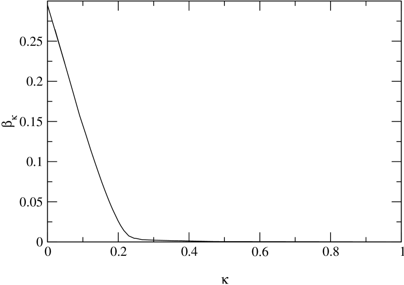
Figure 2: The beta function for $d=2,\ N=2$.

For the nonabelian nonlinear sigma model in $d=2$, $N>2$ there exists an exact expression [89] for the ratio of the renormalized mass $m_{R}$ and the scale $\Lambda_{\overline{MS}}$ which characterizes the two loop running coupling in the $\overline{MS}$ scheme by dimensional transmutation. The flow equation (2.17) together with a choice of the cutoff $R_{k}$ and the initial conditions also defines a renormalization scheme. The corresponding parameter $\Lambda_{ERGE}$ specifies the two loop perturbative value of the running coupling $\kappa^{-1}$ similar to $\Lambda_{\overline{MS}}$ in the $\overline{MS}$ scheme. The numerical solution of the flow equation permits us to compute $m_{R}/\Lambda_{ERGE}$. (Two loop accuracy would be needed for a quantitative determination of $\Lambda_{ERGE}/\Lambda_{\overline{MS}}$.) In table 2 we compare our results with the exact value of $m_{R}/\Lambda_{\overline{MS}}$. The quantitative agreement between $C_{ERGE}$ and $C_{\overline{MS}}$ is striking and suggests $\Lambda_{ERGE}\approx\Lambda_{\overline{MS}}$. We also report the ratio $m_{R}/k_{s}$ with $k_{s}$ defined by $\kappa(k_{s})=0$.

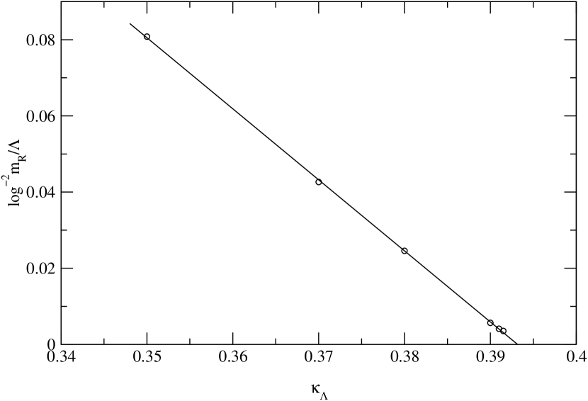
Figure 3: Essential scaling for $d=2,\ N=2$. The renormalized mass $m_{R}$ is plotted as a function of $\kappa_{\Lambda}=\kappa_{\Lambda*}-H(T-T_{c})$.

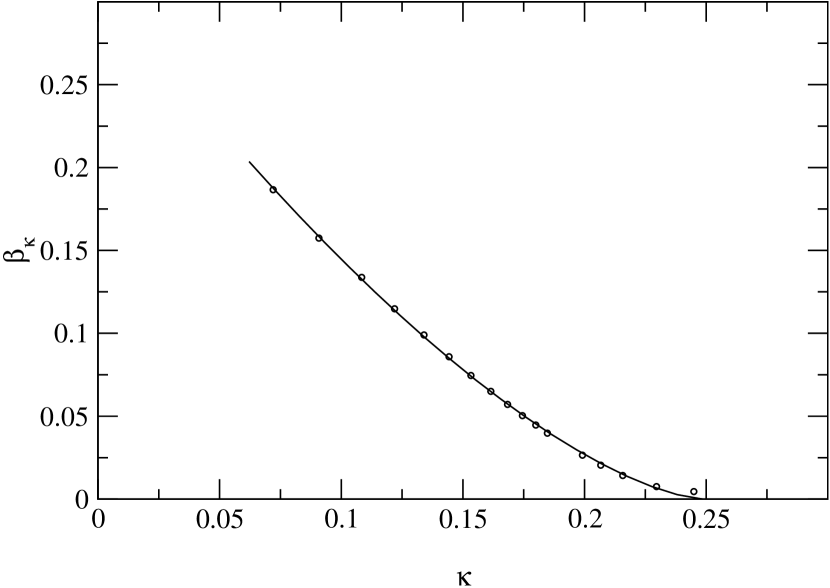
Figure 4: Details of the beta function for $d=2$, $N=2$. The curve is a fit to eq. (3.67).

The abelian case, $N=2$, is known to exhibit a special kind of phase transition which is usually described in terms of vortices [85]. The characteristics of this transition are a massive high temperature phase and a low temperature phase with divergent correlation length but zero magnetization. The anomalous dimension $\eta$ depends on $T$ below $T_{c}$ and is zero above. It takes the exact value $\eta_{*}=0.25$ at the transition. The most distinguishing feature is essential scaling for the temperature dependence of $m_{R}$ just above $T_{c}$,

$$m_{R}\sim e^{-\frac{b}{(T-T_{c})^{\zeta}}},\quad\zeta=\frac{1}{2}.$$ (3.65)

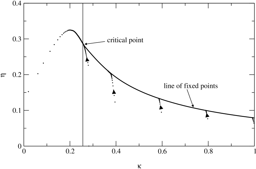
Figure 5: Temperature dependence of the anomalous dimension $\eta$ for the low temperature phase, $d=2$, $N=2$. The line of fixed points is characterized by $\kappa$ and ends in the critical point for the Kosterlitz-Thouless phase transition. We also show the flow towards the line of fixed points and the flow in the high temperature phase away from the critical point (left). The spacing between the points indicates the speed of the flow.

We have already mentioned the existence of a line of fixed points for large values of $\kappa$, which is relevant for the low temperature phase. The contribution of a massless (Goldstone) boson in the renormalization group equation ($w(k)=0$) is responsible for the finite value of $\eta$. This in turn drives the expectation value of the unrenormalized field to zero (even for a nonvanishing renormalized expectation value $\kappa$),

$$\rho_{0}=\kappa/Z_{k}\sim\kappa(k/\Lambda)^{\eta}.$$ (3.66)

We can observe this line of fixed points to a good approximation (cf. fig. 2), although the vanishing of $\beta_{\kappa}$ is not exact (we find $\beta_{\kappa}\approx-4\cdot 10^{-5}\kappa^{-1}+{\cal O}(\kappa^{-2})$). Along the line of fixed points the anomalous dimension $\eta$ differs from zero. This reconciles the massless Goldstone boson with Coleman’s no to theorem [90] for a free propagator. The line of fixed points ends at a phase transition which corresponds to a microscopic parameter $\kappa_{\Lambda*}$ as an initial value of the flow. In order to verify essential scaling we have to examine the flow for values of $\kappa_{\Lambda}$ just below that point, $\kappa_{\Lambda}=\kappa_{\Lambda*}+\delta\kappa_{\Lambda}$, $\delta\kappa_{\Lambda}\sim-(T-T_{c})$. Then $\kappa_{k}$ crosses zero at the scale $k_{s}$ and we find the mass by continuing the flow in the symmetric regime (minimum at $\kappa=0$). In fig. 3 we plot $(\ln{(m_{R}/\Lambda}))^{-2}$ against $\kappa_{\Lambda}$ and find excellent agreement with the straight line (3.65).

How does $\beta_{\kappa}$ have to look like in order to yield essential scaling? Since there is only one independent scale near the transition, one expects $m_{R}(T)=C_{s}k_{s}(T)$, where $k_{s}$ denotes the scale at which $\kappa$ vanishes, i.e. $\kappa(k_{s},T)=0$. For $\kappa$ close to and below $\kappa_{*}$ we parameterize $\beta_{\kappa}$ (this approximation is not valid for very small $\kappa$)

$$\beta_{\kappa}=\frac{1}{\nu}\cdot(\kappa_{*}-\kappa)^{\zeta+1}.$$ (3.67)

For conventional scaling one expects $\zeta=0$ and the correlation length exponent is given by $\nu$. Integrating equation (3.67) yields for $\zeta\neq 0$, $\delta\kappa=\kappa-\kappa_{*}$:

$$\ln(k/\Lambda)=\frac{\nu}{\zeta}\left(\frac{1}{(-\delta\kappa)^{\zeta}}-\frac{1}{(-\delta\kappa_{\Lambda})^{\zeta}}\right).$$ (3.68)

For $k=k_{s}$ the first term $\sim(-\delta\kappa)^{-\zeta}$ is small and independent of $T$ (since $-\delta\kappa(k_{s})=\kappa_{*}$) and equation (3.68) yields the essential scaling relation (3.65) for $\zeta=1/2$. Usually, the microscopic theory is such that one does not start immediately in the vicinity of the critical point and the approximation (3.67) is not valid for $k\approx\Lambda$. However, if one is near the critical temperature the trajectories will stay close to the critical one, $\kappa_{c}(t)$, with $\kappa_{c}(0)=\kappa_{\Lambda*}$. This critical trajectory converges rapidly to its asymptotic value $\kappa_{*}$ and $\beta_{\kappa}$ gets close to eq. (3.67) at some scale $\Lambda^{\prime}<\Lambda$. As a result, one may use equation (3.68) only in its range of validity ($k<\Lambda^{\prime}$) and observe that $\delta\kappa_{\Lambda^{\prime}}$ is also proportional to $T_{c}-T$. The numerical verification of (3.67) is quite satisfactory: Fitting our data yields $\kappa_{*}=0.248$, $\zeta=0.502$ and $\nu^{-1}=2.54$. The uncertainty for $\zeta$ is approximately $\pm 0.05$. The numerical values of $\beta_{\kappa}$ and the approximation (3.67) are shown in fig. 4.

$N$	$\nu$		$\eta$
0	0.70	0.75	0.222	0.2083…
1	0.92	1	0.295	0.25
2	–	–	0.287	0.25

Table 3 Critical exponents $\nu$ and $\eta$ for $d=2$. We compare each value with the exact result.

One can use the information from figure 3 or 4 in order to determine $\kappa_{*}$ and therefore $\eta_{*}=\eta(\kappa_{*})$, the anomalous dimension at the transition. We plot $\eta$ against $\kappa$ in fig. 5. One reads off $\eta_{*}=0.287\pm 0.007$ where the error reflects the two methods used to compute $\kappa_{*}$ and does not include the truncation error. For $\kappa_{\Lambda}>\kappa_{\Lambda*}$ or $T<T_{c}$ the running of $\kappa$ essentially stops after a short “initial running” towards the line of fixed points. One can infer from figure 5 the temperature dependence of the critical exponent $\eta$ for the low temperature phase. In summary all the relevant characteristic features of the Kosterlitz-Thouless transition are visible within our approach.

We also have computed the critical exponents for the “standard” second-order phase transitions for $N=1$ (Ising model) and $N=0$. They are displayed in table 3. The exponents are less accurate than the ones for $d=3$ displayed in table 1 (g). This confirms that the convergence of the derivative expansion is controlled by the size of $\eta$. Nevertheless, the agreement with the exact results is better than 10 %.

We conclude that the first order in the derivative expansion of the exact flow equation for the effective average action gives a quantitatively accurate picture of all phase transitions of scalar models in the $O(N)$ universality class for arbitrary dimension $2\leq d\leq 4$. As the next step, a reliable error estimate would be very welcome.

References

- [1] L.P. Kadanoff, Physica 2 (1966) 263.
- [2] K. G. Wilson, Phys. Rev. B4 (1971) 3174; 3184 K. G. Wilson and I. G. Kogut, Phys. Rep. 12 (1974) 75.
- [3] F. Wegner and A. Houghton, Phys. Rev. A8 (1973) 401; F.J. Wegner in Phase Transitions and Critical Phenomena, vol. 6, eds. C. Domb and M.S. Greene, Academic Press (1976).
- [4] J.F. Nicoll and T.S. Chang, Phys. Lett. A62 (1977) 287; T. S. Chang, D. D. Vvedensky and J. F. Nicoll, Phys. Rep. 217 (1992) 280.
- [5] S. Weinberg, Critical phenomena for field theorists, in Understanding the Fundamental Constituents of Matter, p. 1, Ed. by A. Zichichi (Plenum Press, N.Y. and London, 1978).
- [6] J. Polchinski, Nucl. Phys. B231 (1984) 269;
- [7] A. Hasenfratz and P. Hasenfratz, Nucl. Phys. B270 (1986) 685; P. Hasenfratz and J. Nager, Z. Phys. C37 (1988) 477.
- [8] C. Wetterich, Nucl. Phys. B352 (1991) 529; Z. Phys. C57 (1993) 451; C60 (1993) 461.
- [9] C. Wetterich, Phys. Lett. B301 (1993) 90.
- [10] J. Berges, N. Tetradis, C. Wetterich, hep-ph/0005122.
- [11] C. Bagnuls, C. Bervillier, hep-th/0002034
- [12] J. Berges, N. Tetradis and C. Wetterich, Phys. Rev. Lett. 77 (1996) 873.
- [13] J. Berges and C. Wetterich, Nucl. Phys. B487 (1997) 675.
- [14] S. Seide and C. Wetterich, Nucl. Phys. B562 (1999) 524.
- [15] A. Strumia and N. Tetradis, Nucl. Phys. B542 (1999) 719.
- [16] A. Strumia, N. Tetradis and C. Wetterich, Phys. Lett. B467 (1999) 279.
- [17] T. Morris, Phys. Lett. B345 (1995) 139.
- [18] N. Tetradis and C. Wetterich, Nucl. Phys. B398 (1993) 659; Int. J. Mod. Phys. A9 (1994) 4029.
- [19] B. Bergerhoff, F. Freire, D. Litim, S. Lola, C. Wetterich, Phys. Rev. B53 (1996) 5734; B. Bergerhoff, D. Litim, S. Lola and C.Wetterich, Int. J. Mod. Phys. A11 (1996) 4273.
- [20] N. Tetradis, Nucl. Phys. B488 (1997) 92.
- [21] M. Reuter and C. Wetterich, Nucl. Phys. B408 (1993) 91.
- [22] C. Wetterich, in “Electroweak Physics and the Early Universe”, eds. J. Romao and F. Freire, Plenum Press (1994) 229 (hep-th/9408054).
- [23] J. Berges, D.–U. Jungnickel and C. Wetterich, Phys. Rev. D59 (1999) 034010.
- [24] A. Ringwald, C. Wetterich, Nucl. Phys. B334 (1990), 506.
- [25] N. Tetradis, C. Wetterich, Nucl. Phys. B383 (1992), 197.
- [26] R.D. Ball, P.E. Haagensen, J. Latorre and E. Moreno, Phys. Lett. B347 (1995) 80.
- [27] D.F. Litim, Phys. Lett. B393 (1997) 103; B486 (2000) 92.
- [28] S.-B. Liao, J. Polonyi and M. Strickland, Nucl. Phys. B567 (2000) 493.
- [29] J.-I. Sumi, W. Souma, K.-I. Aoki, H. Terao, and K. Morikawa, hep-th/0002231.
- [30] C. Wetterich, Z. Phys. C48 (1990) 693; S. Bornholdt and C. Wetterich, Phys. Lett. B282 (1992) 399; Z. Phys. C58 (1993) 585.
- [31] J. Comellas, Y. Kubyshin and E. Moreno, Nucl. Phys. B490 (1997) 653.
- [32] M. Reuter, C. Wetterich, Nucl. Phys. B417 (1994) 181
- [33] M. Reuter and C. Wetterich, Nucl. Phys. B391 (1993) 147; B417 (1994) 181; B427 (1994) 291; Phys. Rev. D56 (1997) 7893.
- [34] C. Becchi, Lecture given at the Parma Theoretical Physics Seminar, Sep 1991, preprint GEF-TH-96-11 (hep-th/9607188).
- [35] M. Bonini, M. D’Attanasio, and G. Marchesini, Nucl. Phys. B418 (1994) 81; B421 (1994) 429; B437 (1995) 163; B444 (1995) 602; Phys. Lett. B346 (1995) 87; M. Bonini, G. Marchesini and M. Simionato, Nucl. Phys. B483 (1997) 475.
- [36] U. Ellwanger, Phys. Lett. B335 (1994) 364; U. Ellwanger, M. Hirsch and A. Weber, Z. Phys. C69 (1996) 687; Eur. Phys. J. C1 (1998) 563.
- [37] B. Bergerhoff and C. Wetterich, Nucl. Phys. B440 (1995) 171.
- [38] T.R. Morris, Lectures at the Workshop on the Exact Renormalization Group, Faro, Portugal, Sept. 10-12, 1998 (hep-th/9810104); hep-th/9910058.
- [39] F. Freire, C. Wetterich, Phys. Lett. B380 (1996) 337.
- [40] F. Freire, D. Litim, J. Pawlowski, Phys. Lett. B495 (2000) 256.
- [41] A. Bonanno and D. Zappalà, Phys. Rev. D55 (1997) 6135; M. Reuter, Phys. Rev. D57 (1998) 971; W. Souma, Prog. Theor. Phys. 102 (1999) 181.
- [42] G. Keller, C. Kopper and M. Salmhofer, Helv. Phys. Acta 65 (1992) 32; G. Keller and G. Kopper, Phys. Lett. B273 (1991) 323.
- [43] M. Bonini, M. D’ Attanasio and G. Marchesini, Nucl. Phys. B409 (1993) 441.
- [44] T. R. Morris, Int. J. Mod. Phys. A9 (1994) 2411.
- [45] U. Ellwanger, Z. Phys. C62 (1994) 503.
- [46] U. Ellwanger, Z. Phys. C58 (1993) 619.
- [47] C. Wetterich, Int. J. Mod. Phys. A9 (1994) 3571.
- [48] J. Berges, D.U. Jungnickel, C. Wetterich, hep-ph/9811387.
- [49] N. Tetradis and C. Wetterich, Nucl. Phys. B422 [FS] (1994) 541.
- [50] Yu. M. Ivanchenko, A. A. Lisyansky and A. E. Filippov, Phys. Lett. A150 (1990) 100.
- [51] R. J. Myerson, Phys. Rev. B12 (1975) 2789.
- [52] G. R. Golner, Phys. Rev. B33 (1986) 7863.
- [53] T. R. Morris and J. F. Tighe, JHEP 9908 (1999) 007.
- [54] K.-I. Aoki, K. Morikawa, W. Souma, J.-I. Sumi and H. Terao, Prog. Theor. Phys. 99 (1998) 451.
- [55] K. I. Aoki, K. Morikawa, W. Souma, J.-I. Sumi and H. Terao, Prog. Theor. Phys. 95 (1996) 409.
- [56] A. Margaritis, G. Ódor and A. Patkós, Z. Phys. C39 (1988) 109.
- [57] P. E. Haagensen, Y. Kubyshin, J. I. Latorre and E. Moreno, Phys. Lett. B323 (1994) 330.
- [58] T. Morris, Phys. Lett. B334 (1994) 355.
- [59] F.J. Dyson, Phys. Rev. 75 (1949) 1736; J. Schwinger, Proc. Nat. Acad. Sc. 37 (1951) 452.
- [60] J. Adams, J. Berges, S. Bornholdt, F. Freire, N. Tetradis and C. Wetterich, Mod. Phys. Lett. A10 (1995) 2367.
- [61] J. F. Nicoll, T. S. Chang and H. E. Stanley, Phys. Rev. Lett. 33 (1974) 540; Phys. Rev. A13 (1976) 1251.
- [62] J. F. Nicoll and T. S. Chang, Phys. Rev. A17, 2083 (1978).
- [63] J. Comellas and A. Travesset, Nucl. Phys. B498 (1997) 539.
- [64] T. Papenbrock and C. Wetterich, Z. Phys. C65 (1995) 519.
- [65] G. Felder, Com. Math. Phys. 111 (1987) 101.
- [66] A. E. Filippov and S. A. Breus, Phys. Lett. A158 (1991) 300; S. A. Breus and A. E. Filippov, Physica A192 (1993) 486; A. E. Filippov, Theor. Math. Phys. 91 (1992) 551.
- [67] T. Morris, Phys. Lett. B329 (1994) 241.
- [68] D. Litim, private communication.
- [69] N. Tetradis and D. F. Litim, Nucl. Phys. B464 [FS] (1996) 492.
- [70] K.G. Wilson and M.E. Fisher, Phys. Rev. Lett. 28 (1972) 240.
- [71] R. Guida and J. Zinn-Justin, J. Phys. A31 (1998) 8103; J. Zinn-Justin, hep-th/0002136.
- [72] I. Kondor and T. Temesvari, J. Phys. Lett. (Paris) 39 (1978) L99.
- [73] P. Butera and M. Comi, Phys. Rev. B56 (1997) 8212.
- [74] M. Campostrini, A. Pelissetto, P. Rossi and E. Vicari, Phys. Rev. E60 (1999) 3526; Phys. Rev. B61 (2000) 5905.
- [75] J. Zinn-Justin, hep-th/0002136.
- [76] T. Reisz, Phys. Lett. B360 (1995) 77.
- [77] S.Y. Zinn, S.N. Lai, M.E. Fisher, Phys. Rev. E54 (1996) 1176.
- [78] B. Li, N. Madras, A.D. Sokal, J. Statist. Phys. 80 (1995) 661.
- [79] H.G. Ballesteros, L.A. Fernandez, V. Martin-Mayor, A. Munoz Sudupe, Phys. Lett. B387 (1996) 125 (values for quoted from [71]).
- [80] M. Hasenbusch, K. Pinn and S. Vinti, Phys. Rev. B59 (1999) 11471; M. Hasenbusch and T. Török, J. Phys. A32 (1999) 6361.
- [81] J. Engels and T. Mendes, Nucl. Phys. B572 (2000) 289.
- [82] G. v. Gersdorff and C. Wetterich, hep-th/0008114.
- [83] M. Alford, Phys. Lett. B336 (1994) 237.
- [84] T.R. Morris and M.D. Turner, Nucl. Phys. B509 (1998) 637; T. R. Morris, Nucl. Phys. B495 (1997) 477; T. R. Morris, Int. J. Mod. Phys. B12 (1998) 1343.
- [85] J.M. Kosterlitz and D.J. Thouless, J. Phys. C6 (1973) 1181; J.M. Kosterlitz, J. Phys. C7 (1974) 1046.
- [86] N.D. Mermin and H. Wagner, Phys. Rev. Lett. 17 (1966) 1133.
- [87] M. Gräter and C. Wetterich, Phys. Rev. Lett. 75 (1995) 378.
- [88] A.M. Polyakov, Phys. Lett. B59 (1975) 79; A. d’Adda, M. Lüscher and P. di Vecchia, Nucl. Phys. B146 (1978) 63; E. Witten, Nucl. Phys. B149 (1979) 285; S. Hikami and E. Brezin, J. Phys. A11 (1978) 1141; W. Bernreuther and F. Wegner, Phys. Rev. Lett. 57 (1986) 1383.
- [89] P. Hasenfratz, M. Maggiore, and F. Niedermayer, Phys. Lett. B245, 522 (1990); P. Hasenfratz and F. Niedermayer, Phys. Lett. B245, 529 (1990).
- [90] S. Coleman, Comm. Math. Phys. 31 (1973) 259.