Interplay between perturbative and non-perturbative QCD in three-jet events

Abstract

We present the perturbative (PT) and non-perturbative (NP) analysis of the cumulative out-of-event-plane momentum distribution in $e^{+}e^{-}$ annihilation in the near-to-planar three-jet region. A physical interpretation based on simple QCD considerations and kinematical relations will be given, with the aim of extending the described techniques to other multi-jet processes and, possibly, to hadron-hadron collisions.

1 Introduction

Hadronic multi-jet events play a crucial rôle both in the context of precision tests of QCD and in the search for new physics, so that it has become essential to reach, in the analysis of multi-jet configurations, the same theoretical accuracy as in two-jet events. As a first step in this direction we aim to extend the “state-of-the-art ” of two-jet event shape variables such as Thrust (T), C-parameter, Broadening (B), to three-jet event shapes. This standard analysis consists in a resummed single logarithmic (SL) prediction, the exact fixed order result, the matching of the two and the non-perturbative power corrections.

We present here the (Thrust) Minor distribution, which gives a measure of the aplanarity of a three-jet event. The final answer is rather involved, since it reveals the rich colour and geometry structure of the hard underlying process ($e^{+}e^{-}\rightarrow q\,\bar{q}\,g$).

The aim of this paper is to present only the main features of the Minor distribution, while all computational details may be found in a separate paper.[1] In section 2 we introduce the observable and the distribution. The physical interpretation of the SL resummed PT result is explained in section 3. Section 4 is devoted to the power corrections. We conclude in section 5 giving some outlooks.

2 Observable and kinematics

The (Thrust) Minor ($T_{m}$) gives a measure of the cumulative out-of-event-plane momentum $K_{\mbox{\scriptsize out}}$:

$$T_{m}\,Q=\sum_{i}\left|\>{p}_{ix}\>\right|\>\equiv\>K_{\mbox{\scriptsize out}}\>.$$ (1)

Here Q is the centre-of-mass energy, the sum is over all hadrons and we have fixed the z- and the y-axis along the thrust ($T$) and the thrust-major ($T_{M}$) axes respectively[2].

At Born level a three-jet event consists of a quark, an antiquark and a hard, non-collinear gluon. For kinematical reasons these partons lie in a plane, so that $K_{\mbox{\scriptsize out}}=0$. We denote by $p_{a}$ the energy ordered ($p_{1}^{0}>p_{2}^{0}>p_{3}^{0}$) parton momenta. There are essentially three Born configurations: we denote by $\delta$ ($\delta=1,2,3$) the configuration in which the momentum of the hard gluon is $p_{\delta}$ (see Fig. 1).

Figure 1: The three Born configurations ordered according to decreasing probability.

Beyond Born level one can study the “integrated” $K_{\mbox{\scriptsize out}}$-distribution $\Sigma_{\delta}(K_{\mbox{\scriptsize out}})$, defined by

$$\frac{d\sigma_{\delta}(T,T_{M},K_{\mbox{\scriptsize out}})}{dT\>dT_{M}\>dK_{\mbox{\scriptsize out}}}\equiv\>M_{\delta}^{2}(T,T_{M})\frac{d{\cal{V}}_{\delta}(K_{\mbox{\scriptsize out}})}{dK_{\mbox{\scriptsize out}}}\>,$$ (2)

$${\cal{V}}_{\delta}(K_{\mbox{\scriptsize out}})\equiv{\cal{C}}(\alpha_{\mbox{\scriptsize s}})\Sigma_{\delta}(K_{\mbox{\scriptsize out}})+{\cal{D}}_{\delta}(K_{\mbox{\scriptsize out}})\>.$$ (3)

Here $M_{\delta}^{2}(T,T_{M})$ denotes the hard matrix element for the production of a quark-antiquark-gluon ensemble in the configuration $\delta$ for fixed $T$ and $T_{M}$. $\Sigma_{\delta}(K_{\mbox{\scriptsize out}})$ resums all double (DL) and all single logarithms (SL). Hard emitted parton contributions[3] are embodied both in the “coefficient function” ${\cal{C}}(\alpha_{\mbox{\scriptsize s}})$, which has an expansion in powers of $\alpha_{\mbox{\scriptsize s}}(Q)$, and in the “remainder function” ${\cal{D}}(K_{\mbox{\scriptsize out}})$, which vanishes for $K_{\mbox{\scriptsize out}}\rightarrow 0$.

3 PT result

The PT resummed result to SL accuracy has the following structure[1]

$$\Sigma_{\delta}(K_{\mbox{\scriptsize out}})=e^{-R(K_{\mbox{\scriptsize out}})}\cdot{\cal{S}}_{\delta}(K_{\mbox{\scriptsize out}})\>.$$ (4)

Here $R$ is a DL function which resums all soft and collinear parton emissions,

$$R(K_{\mbox{\scriptsize out}})=\sum_{a}C_{a}\int_{K_{\mbox{\scriptsize out}}}^{Q_{a}^{\mbox{\scriptsize PT}}}\frac{dk_{x}}{k_{x}}\frac{2\alpha_{\mbox{\scriptsize s}}(2k_{x})}{\pi}\ln\frac{Q_{a}^{\mbox{\scriptsize PT}}}{k_{x}}\stackrel{{\scriptstyle DL}}{{\longrightarrow}}C_{T}\frac{\alpha_{\mbox{\scriptsize s}}(Q)}{\pi}\ln^{2}\frac{Q}{K_{\mbox{\scriptsize out}}}\>,$$ (5)

where $C_{a}$ is the colour charge of parton $\#a$ ($C_{\delta}=C_{A},C_{a}=C_{F}$ for $a\neq\delta$) and $C_{T}=2C_{F}+C_{A}$ is the total colour charge of the hard quark-antiquark-gluon ensemble. Sources of SL corrections in $R$ are the running of the coupling, corrections due to hard collinear splittings and the dependence on the geometry through the three hard momentum scales $Q_{a}^{\mbox{\scriptsize PT}}$. Each of these scales has a nice geometrical interpretation: for the quark or the antiquark it is (proportional to) the $q\bar{q}$ invariant mass, for the hard gluon it is (proportional to) its invariant transverse momentum with respect to the $q\bar{q}$ dipole.

The remaining SL corrections, in particular those due to hard parton recoil, are embodied in the SL function ${\cal{S}}$. At first order in $\alpha_{\mbox{\scriptsize s}}$ (one secondary gluon emission), ${\cal{S}}$ is given by

$${\cal{S}}=1-\frac{2\alpha_{\mbox{\scriptsize s}}}{\pi}\ln\frac{Q}{K_{\mbox{\scriptsize out}}}(2C_{1}+C_{2}+C_{3})\ln 2\>.$$ (6)

This shows that the contribution to $K_{\mbox{\scriptsize out}}$ due to emission from the parton along the thrust axis ($p_{1}$) is twice the contribution of each of the remaining two emitters. There is a simple kinematical reason for this.[1] Indeed the definition of the $T$- and $T_{M}$-axes implies that when the secondary gluon $k$ is emitted from $p_{1}$ (see Fig. 2b) all three hard partons experience equal out-of-plane recoils,

$$k_{z}>0,\quad k_{y}>0:\quad p_{1x}=-k_{x}=p_{2x}=-p_{3x}\quad$$

$$k_{y}<0:\quad p_{1x}=-k_{x}=-p_{2x}=p_{3x}\>,$$

so that $K_{\mbox{\scriptsize out}}=4\cdot\left|\>k_{x}\>\right|$. On the other hand, when the secondary gluon is emitted from $p_{2}$ or $p_{3}$ (see Fig. 2c or d) only one hard parton recoils against it:

$$k_{z}<0,\quad k_{y}>0:\quad p_{2x}=-k_{x};\>\>p_{1x}=p_{3x}=0\quad$$

$$k_{y}<0:\quad p_{3x}=-k_{x};\>\>p_{1x}=p_{2x}=0\>,$$

so that $K_{\mbox{\scriptsize out}}=2\cdot|k_{x}|$.

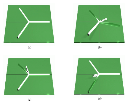
Figure 2: (a) Hard partons in a generic Born configuration. (b) Soft gluon $k$ (the short curly stick) is emitted from $p_{1}$. All three hard partons experience equal out-of-plane recoils, see Eq.3. White (shadowed) partons have positive (negative) $x$-components of the momentum. (c) Soft gluon $k$ is emitted from $p_{2}$. According to Eq.3, only parton #2 recoils (shadowed; has a negative $x$-component of the momentum), parton #1 and #3 (white) remain in the event plane. (d) The case of $k$ emitted from $p_{3}$.

4 NP result

Power corrections arise because of emission of extra-soft gluons with transverse momentum of order $\Lambda_{QCD}$. In this phase space region a pure PT approach is not possible. In fact, due to the growth of the PT coupling at low scales, the PT series have a factorial behaviour, see a recent review for details. [4] These effects (both PT and NP) are needed for precision tests of QCD and are a way to explore low energy regions.

The Ansatz we start from is that there exists an IR-finite running coupling defined at all scales in terms of a dispersive representation à la DMW.[5] For a generic $e^{+}e^{-}$ event shape variable ($V$) power corrections result in a shift of the PT distribution

$$\Sigma(V)=\Sigma^{\mbox{\scriptsize PT}}(V-\delta V)\>.$$ (9)

The NP part of the shift has the following general form[6]:

$$\delta V=\rho(V){\cal{M}}\frac{\mu_{I}\alpha_{0}}{Q}+{\cal{O}}\left(\alpha_{\mbox{\scriptsize s}}(Q)\frac{\mu_{I}}{Q}\right)\qquad\alpha_{0}(\mu_{I})=\frac{1}{\mu_{I}}\int_{0}^{\mu_{I}}\!dk\,\alpha_{s}(k)\>.$$ (10)

Here $\alpha_{0}$ is the universal parameter which measures the strength of the strong interaction at low scales: it is the mean value of the full coupling constant (PT and NP) below a certain merging scale. ${\cal{M}}$ is the Milan factor which takes into account two-loop corrections in a universal way. The coefficient function $\rho(V)$ is specific of the observable considered and can be computed via PT calculations.

As in the case of Broadening[7], the shift of the Minor distribution depends logarithmically on the hard parton recoil momenta ($p_{ax}$)

$$\Delta K_{\mbox{\scriptsize out}}\sim\sum_{a}C_{a}\ln\frac{Q}{|p_{ax}|}\>,$$ (11)

so that, once the shift $\Delta(K_{\mbox{\scriptsize out}})$ in a generic PT configuration is known, the total shift is given by the average of its expression over the PT recoil distribution:

$$\delta K_{\mbox{\scriptsize out}}\,=\,\langle\Delta K_{\mbox{\scriptsize out}}\rangle\>_{\mbox{\scriptsize PT}}\>.$$ (12)

There are two interesting limiting cases, the region of well developed (multiple) PT radiation, i.e. $\alpha_{\mbox{\scriptsize s}}\ln^{2}(K_{\mbox{\scriptsize out}}/Q)\gg 1$ and the phase space region with only few hard PT partons, i.e. $\alpha_{\mbox{\scriptsize s}}\ln^{2}(K_{\mbox{\scriptsize out}}/Q)\ll 1$.

In the first case all three hard partons have similar recoils ($p_{ax}\sim K_{\mbox{\scriptsize out}}$) and the shift results in

$$\delta K_{\mbox{\scriptsize out}}\sim C_{T}\ln\frac{Q}{K_{\mbox{\scriptsize out}}}\>.$$ (13)

In the second case the shift depends on which hard parton controls the PT emission and therefore the recoil. It is therefore useful to single out in the total shift the contribution of each hard parton:

$$\delta K_{\mbox{\scriptsize out}}=\sum_{a}\frac{C_{a}}{C_{T}}\delta K_{\mbox{\scriptsize out}}^{(a)}\>.$$ (14)

Here $C_{a}/C_{T}$ represents (roughly) the probability that PT radiation is due to emission from parton $\#a$.

• PT emission from $p_{1}$: all three hard partons have similar out-of-plane recoils (see Eq.3), so that, as in the previous case, $p_{ax}\sim K_{\mbox{\scriptsize out}}$ and the shift is a logarithm

  $$\delta K_{\mbox{\scriptsize out}}^{(1)}\sim(2C_{F}+C_{A})\ln\frac{Q}{K_{\mbox{\scriptsize out}}}\>.$$ (15)

• PT emission from $p_{2}$: only the out-of-plane momentum $p_{2x}$ is fixed by PT radiation (see Eq.3), so that $p_{2x}\sim K_{\mbox{\scriptsize out}}$ and one has to integrate over the PT distribution of the other two “free” hard partons:

  $$\delta K_{\mbox{\scriptsize out}}^{(2)}\sim\frac{C_{F}}{\sqrt{\alpha_{\mbox{\scriptsize s}}C_{F}}}+C_{F}\ln\frac{Q}{K_{\mbox{\scriptsize out}}}+\frac{C_{A}}{\sqrt{\alpha_{\mbox{\scriptsize s}}(C_{F}+C_{A})}}\>.$$ (16)

  In this case the shift contains a $1/\sqrt{\alpha_{\mbox{\scriptsize s}}}$ enhancement coming from the average of $\ln Q/p_{ax}$ ($a=1,3$) in Eq. 11 over the corresponding DL Sudakov form factor.[1] Similar considerations hold for PT emission from $p_{3}$.

5 Conclusions and outlook

Special features of Thrust Minor distributions are the richness of the geometry dependent structure and the sensitivity to large angle soft gluon emissions.

The next step will be to extend this calculation to hadron-hadron collisions, where one has to take into account effects due to initial state radiation.

References

-
[1]
A. Banfi, Yu.L. Dokshitzer, G. Marchesini and
G. Zanderighi, JHEP 07, 002 (2000), [hep-ph/0004027];
A. Banfi, Yu.L. Dokshitzer, G. Marchesini and G. Zanderighi, [hep-ph/0010267]. -
[2]
DELPHI Coll., Eur. Phys. J. C 14, 557 (2000),
[hep-ex/0002026];
OPAL Coll., Eur. Phys. J. C 16, 185 (2000), [hep-ex/0002012];
L3 Coll., Phys. Lett. B 489, 65 (2000), [hep-ex/0005045]. - [3] S. Catani, L. Trentadue, G. Turnock and B.R. Webber, Nucl. Phys. B 407, 3 (1993);
- [4] M. Beneke, Phys. Rep. 317, 1 (1999), [hep-ph/9807443], and references therein.
- [5] Yu.L. Dokshitzer, G. Marchesini and B.R. Webber, Nucl. Phys. B 469, 93 (1996), [hep-ph/9512336].
- [6] Yu.L. Dokshitzer, A. Lucenti, G. Marchesini and G.P. Salam, Nucl. Phys. B 511, 396 (1998), [hep-ph/9707532]. Yu.L. Dokshitzer, A. Lucenti, G. Marchesini and G.P. Salam, JHEP 05, 003 (1998), [hep-ph/9802381].
- [7] Yu.L. Dokshitzer, G. Marchesini and G.P. Salam, Eur. Phys. J. C 3, 1 (1999), [hep-ph/9812487].