Topics on four-fermion Physics at electron-positron colliders 111Invited talk presented at QFTHEP’2000, Tver, Russia.

Roberto Pittau

Dipartimento di Fisica Teorica, Università di Torino, Italy

INFN, Sezione di Torino, Italy

Abstract

I review the most recent progresses in the calculation of four-fermion processes in $e^{+}e^{-}$ collisions.

Introduction

Final state four-fermion processes represent an important ingredient when studying high energy $e^{+}$ $e^{-}$ collisions. They enter in the analysis of the $Z$-peak observables at LEP, as (mainly) QED pair corrections to 2-fermion processes. Such a set of contributions, together with the full set of electroweak (EW) loop corrections, allows very stringent tests the Standard Model (SM) at the radiative level.

At LEP2 energies, all relevant signatures such as $WW$, $ZZ$, single-$W$, single-$Z$ and Higgs production manifest themselves as four-fermion final states. These same processes are also relevant for precision measurements at the Linear Collider (LC) and as a SM background to searches.

In the following, based on the CERN Report of ref. [1], I review the most recent achievements in the computation of four-fermion processes. Table 1 contains a list of contributing codes. Emphasis is put here on the available tools for estimating the theoretical errors to be associated with the four-fermion observables, in view of the final LEP analysis, but also on the improvements needed at the LC.

The first two sections are devoted to $W$-pair and single-$W$ signatures, while, in the last two parts, I cover topics on four-fermion production plus 1 visible photon and $Z$-pair final states.

Code       Authors
BBC [2]     F. Berends, W Beenakker and A. Chapovsky
CompHEP [3]     E. Boos, M. Dubinin and V. Ilyin
GENTLE [4]     D. Bardin, A. Olchevsky and T. Riemann
GRACE [5]     Y. Kurihara, M. Kuroda and Y. Shimizu
KORALW/YFSWW [6]     S. Jadach, W. Placzek, M. Skrypek, B. Ward and Z. Was
NEXTCALIBUR [7]     F. Berends, C. G. Papadopoulos and R. Pittau
PHEGAS/HELAC [8]     C. G. Papadopoulos
RACOONWW [9]     A. Denner, S. Dittmaier, M. Roth and D. Wackeroth
SWAP [10]     G. Montagna, M. Moretti, O. Nicrosini, A. Pallavicini and F. Piccinini
WPHACT [11]     E. Accomando, A. Ballestrero and E. Maina
WRAP [10]     G. Montagna, M. Moretti, O. Nicrosini, M. Osmo and F. Piccinini
WTO [12]     G. Passarino
YFSZZ [13]     S. Jadach, W. Placzek and B.F.L. Ward
ZZTO [14]     G. Passarino
Table 1: Contributing programs.

1 $W$-pair production

When collecting data at $\sqrt{s}=$ 189 GeV, the LEP2 collaborations observed a deficit in the number of events, with respect to the SM predictions. This fact triggered a re-analysis of the available tools for calculating the total cross section $\sigma_{WW}$. At that time, a theoretical 2% error band was assigned to this observable, two times bigger than the experimental error. The estimate of the theoretical error was based on the GENTLE/4FAN inclusion of QED Initial State Radiation (ISR), without any attempt to take EW contributions into account. Therefore, it was immediately clear that the computation of the genuine EW effects was needed to match the experimental accuracy. On the other hand a full four-fermion one-loop EW calculation was (and still is) beyond reach, and including only the $WW$-like diagrams violates gauge invariance. The solution to this problem is represented by the so called Double Pole Approximation (DPA) [15]. The DPA isolates the poles at the complex squared masses, with gauge invariant residues which are then projected onto the respective on-shell gauge invariant counterparts. The projection is from the off-shell phase space to the on-shell phase space. Even though such a procedure is strictly gauge invariant, the projection procedure is not unique. However, the ambiguity is small, namely ${\cal O}(\frac{\alpha}{\pi}\frac{\Gamma_{W}}{M_{W}})$.

For example, in the case of a single unstable particle, the fully re-summed amplitude can be rewritten as follows

$\displaystyle{\cal M}^{\infty}$ $\displaystyle=$ $\displaystyle\frac{W(p^{2},\omega)}{p^{2}-\tilde{M}^{2}}\,\sum_{n=0}^{\infty}\,\Biggl{(}\frac{-\tilde{\Sigma}(p^{2})}{p^{2}-\tilde{M}^{2}}\Biggr{)}^{n}=\ \frac{W(p^{2},\omega)}{p^{2}-\tilde{M}^{2}+\tilde{\Sigma}(p^{2})}$ (1)
$\displaystyle=$ $\displaystyle\frac{W(M^{2},\omega)}{p^{2}-M^{2}}\,\frac{1}{Z(M^{2})}+\Biggl{[}\frac{W(p^{2},\omega)}{p^{2}-\tilde{M}^{2}+\tilde{\Sigma}(p^{2})}-\frac{W(M^{2},\omega)}{p^{2}-M^{2}}\,\frac{1}{Z(M^{2})}\Biggr{]}$
$\displaystyle M^{2}-\tilde{M}^{2}+\tilde{\Sigma}(M^{2})=0,\quad\quad Z(M^{2})=1+\tilde{\Sigma}^{\prime}(M^{2}),$

where $\tilde{M}$ and $M$ are the bare mass and the complex pole of the instable particle, and $Z$ the wave-function factor. The first term is the gauge invariant single-pole residue (on-shell production and decay of the unstable particle). The second term has no pole and can be in principle expanded in powers of $\,p^{2}-M^{2}$.

Applying DPA to $W$-pair production means that only the double-pole residues of the two resonances are considered, and one-loop EW contributions included there, for which only (available) on-shell corrections are needed. The corrections to be included fall in two different classes, namely factorizable contributions, in which the production, propagation and decay steps are clearly separated, and non-factorizable contributions, in which a photon with energy $E_{\gamma}\mathrel{\raisebox{-3.00003pt}{$\stackrel{{\scriptstyle\displaystyle<}}{{\sim}}$}}\Gamma_{W}$ is emitted (see figure 1).

\SetScale

0.7 \Text(-30,92)[lc](a) \ArrowLine(43,58)(25,40) \Text(7,40)[lc]$e^{+}$\ArrowLine(25,90)(43,72) \Text(7,92)[lc]$e^{-}$\Photon(50,65)(150,95)112 \Text(100,105)[]$W$\Photon(50,65)(150,35)112 \Text(100,25)[]$W$\ArrowLine(155,98)(175,110) \Text(190,110)[rc]$f_{1}^{\prime}$\ArrowLine(175,80)(155,92) \Text(190,80)[rc]$\bar{f}_{1}$\ArrowLine(175,50)(155,38) \Text(190,50)[rc]$\bar{f}_{2}^{\prime}$\ArrowLine(155,32)(175,20) \Text(190,20)[rc]$f_{2}$\DashLine(75,115)(75,15)5 \Text(40,5)[]production \DashLine(125,115)(125,15)5 \Text(150,5)[]decays \GCirc(50,65)101 \GCirc(100,80)100.8 \GCirc(100,50)100.8 \GCirc(150,95)101 \GCirc(150,35)101

\SetScale

0.7 \Text(-30,92)[lc](b) \ArrowLine(30,50)( 5, 95) \ArrowLine( 5, 5)(30, 50) \Photon(30,50)(90,80)26 \Photon(30,50)(90,20)26 \GCirc(30,50)100 \Vertex(90,80)1.2 \Vertex(90,20)1.2 \ArrowLine(90,80)(120, 95) \ArrowLine(120,65)(105,72.5) \ArrowLine(105,72.5)(90,80) \Vertex(105,72.5)1.2 \ArrowLine(120, 5)( 90,20) \ArrowLine( 90,20)(105,27.5) \ArrowLine(105,27.5)(120,35) \Vertex(105,27.5)1.2 \Photon(105,27.5)(105,72.5)24.5 $\gamma$ $W$ $W$   \ArrowLine(30,50)( 5, 95) \ArrowLine( 5, 5)(30, 50) \Photon(30,50)(90,80)26 \Photon(30,50)(90,20)26 \Vertex(60,35)1.2 \GCirc(30,50)100 \Vertex(90,80)1.2 \Vertex(90,20)1.2 \ArrowLine(90,80)(120, 95) \ArrowLine(120,65)(105,72.5) \ArrowLine(105,72.5)(90,80) \Vertex(105,72.5)1.2 \ArrowLine(120, 5)(90,20) \ArrowLine(90,20)(120,35) \Photon(60,35)(105,72.5)25 $\gamma$ $W$ $W$ $W$   \ArrowLine(30,50)( 5, 95) \ArrowLine( 5, 5)(30, 50) \Photon(30,50)(90,80)-26 \Photon(30,50)(90,20)26 \Vertex(60,65)1.2 \GCirc(30,50)100 \Vertex(90,80)1.2 \Vertex(90,20)1.2 \ArrowLine(90,80)(120, 95) \ArrowLine(120,65)(105,72.5) \ArrowLine(105,72.5)(90,80) \Vertex(105,27.5)1.2 \ArrowLine(120, 5)(90,20) \ArrowLine(105,27.5)(120,35) \ArrowLine(90,20)(105,27.5) \Photon(60,65)(105,27.5)-25 $\gamma$ $W$ $W$ $W$
\SetScale0.7 \ArrowLine(30,50)( 5, 95) \ArrowLine( 5, 5)(30, 50) \Photon(30,50)(90,80)26 \Photon(30,50)(90,20)26 \GCirc(30,50)100 \Vertex(90,80)1.2 \Vertex(90,20)1.2 \ArrowLine(90,80)(120, 95) \ArrowLine(120,65)(105,72.5) \ArrowLine(105,72.5)(90,80) \ArrowLine(120, 5)( 90,20) \ArrowLine( 90,20)(120,35) \Vertex(105,72.5)1.2 \PhotonArc(120,65)(15,150,270)23 $W$ $W$ $\gamma$\DashLine(120,0)(120,100)6 \PhotonArc(120,35)(15,-30,90)23 \Vertex(135,27.5)1.2 \ArrowLine(150,80)(120,95) \ArrowLine(120,65)(150,80) \ArrowLine(120, 5)(150,20) \ArrowLine(150,20)(135,27.5) \ArrowLine(135,27.5)(120,35) \Vertex(150,80)1.2 \Vertex(150,20)1.2 \Photon(210,50)(150,80)26 \Photon(210,50)(150,20)26 \ArrowLine(210,50)(235,95) \ArrowLine(235, 5)(210,50) \GCirc(210,50)100 $W$ $W$

Figure 1: Factorizable (a) and non factorizable (b) contributions to $W$-pair production.

The DPA is not reliable at the $W$-pair threshold, where the background diagrams get important. The expected DPA uncertainty above threshold is of the order ${\cal O}\left(\frac{\alpha}{\pi}\frac{\Gamma_{W}}{M_{W}}{\rm ln(\cdots)}\right)\,<0.5\%$, in fact, when $\sqrt{s}>2\,M_{W}+n\Gamma_{W}$ with $n={\cal O}(3-5)$, the background diagrams are of the order $\sim\frac{\alpha}{\pi}\frac{\Gamma_{W}}{\sqrt{s}-M_{W}}\,{\rm ln(\cdots)}\sim 0.1\%$.

Very far away from resonance, the DPA cannot be used any more.

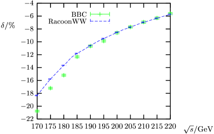
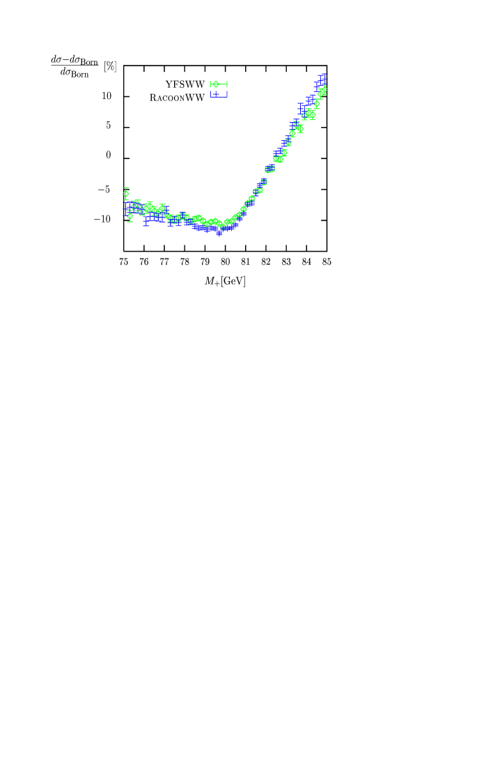
At LEP2 energies, the inclusion of the DPA formalism in RACOONWW, BBC and YFSWW allows to lower the theoretical uncertainty on $\sigma_{WW}$ from 2% to 0.5 %, in much better agreement with the data. In figures 2 and 3 and table 2 we show examples of comparisons among the codes.

Refer to caption

Figure 2: Relative ${\cal O}({\alpha})$ corrections to $\sigma(e^{+}e^{-}\to\nu_{\mu}\mu^{+}\tau^{-}\bar{\nu}_{\tau})$.
no cuts $\sigma_{\mathrm{tot}}[\mathrm{fb}]$
final state program Born best
YFSWW3 219.770(23) 199.995(62)
$\nu_{\mu}\mu^{+}\tau^{-}\bar{\nu}_{\tau}$ RacoonWW 219.836(40) 199.551(46)
(Y–R)/Y $-0.03(2)$% 0.22(4)%
YFSWW3 659.64(07) 622.71(19)
$u\bar{d}\mu^{-}\bar{\nu}_{\mu}$ RacoonWW 659.51(12) 621.06(14)
(Y–R)/Y $0.02(2)$% 0.27(4)%
YFSWW3 1978.18(21) 1937.40(61)
$u\bar{d}s\bar{c}$ RacoonWW 1978.53(36) 1932.20(44)
(Y–R)/Y $-0.02(2)$% 0.27(4)%
Table 2: Total cross section at $\sqrt{s}=200\,{\rm GeV}$ without cuts.

In conclusion, with the help of the DPA, a theoretical accuracy at the level of 0.5 % on $\sigma_{WW}$ is reached, as required by the LEP2 collaborations [1]. The error decreases with increasing energy, giving the following estimates of the theoretical uncertainty on $\sigma_{\rm WW}$

  • 0.4 % at $\sqrt{s}=200$ GeV,  0.5 % at $\sqrt{s}=180$ GeV,  0.7 % at $\sqrt{s}=170$ GeV.

A theoretical uncertainty of the order of 1 % must be assigned to the distributions.

A full four-fermion one-loop EW calculation is still missing, but it is required for high precision measurements at the LC.

Refer to caption

Figure 3: Distribution in the $W^{+}$ invariant mass at $\sqrt{s}=200\,{\rm GeV}$ for the $u\bar{d}\mu^{-}\bar{\nu}_{\mu}$ final state.

2 Single-$W$ production

The experimental single-$W$ signature is better defined with the help of table 3.

Process diagrams cuts
$ee\nu\nu$ $t$-channel only $E(e^{+})>20\,GeV,|\cos\theta(e^{+})|<0.95$
$e\nu\mu\nu$ $t$-channel only $E_{(}\mu^{+})>20\,GeV$
$e\nu\tau\nu$ $t$-channel only $E_{(}\tau^{+})>20\,GeV$
$e\nu ud$ $t$-channel only $M(ud)>45GeV$
$e\nu cs$ $t$-channel only $M(cs)>45GeV$
Table 3: Possible single-$W$ processes. $|\cos\theta(e^{-})|>0.95$.

The contributing Feynman diagrams can be split into $s$-channel and $t$-channel amplitudes, as depicted in figure 4.

\SetOffset(50,0) \ArrowLine(50,50)(0,100) \ArrowLine(100,100)(50,50) \ArrowLine(0,0)(50,50) \ArrowLine(50,50)(100,0) \ArrowLine(100,70)(50,50) \ArrowLine(50,50)(100,30) \GCirc(50,50)150.5 \Text(10,100)[lc]$e^{+}$\Text(10,0)[lc]$e^{-}$\Text(110,100)[lc]$\bar{\nu}_{e}$\Text(110,70)[lc]$\bar{f}_{2}$\Text(110,30)[lc]$f_{1}$\Text(110,0)[lc]$e^{-}$\Text(65,-20)[t]$s$-channel
\SetOffset(150,0) \ArrowLine(50,50)(0,100) \ArrowLine(100,100)(50,50) \ArrowLine(100,70)(50,50) \ArrowLine(50,50)(100,30) \Photon(50,50)(50,10)27 \ArrowLine(0,0)(50,10) \ArrowLine(50,10)(100,0) \GCirc(50,50)150.5 \Text(10,100)[lc]$e^{+}$\Text(10,-5)[lc]$e^{-}$\Text(110,100)[lc]$\bar{\nu}_{e}$\Text(110,70)[lc]$\bar{f}_{2}$\Text(110,30)[lc]$f_{1}$\Text(110,-5)[lc]$e^{-}$\Text(65,-20)[t]$t$-channel \Text(60,20)[lc]$t$\Text(-40,50)[lc]$+$
Figure 4: $s$-channel and $t$-channel diagrams in single-$W$ production.

Only the $t$-channel contribution is included in the definition of the single-$W$ processes. This set is explicitly drawn, for the $e\nu ud$ final state, in figure 5. The reason of this diagram based definition is that it allows an easy combination of different processes from different experiments. Notice that, in order to preserve gauge invariance, all $t$-channel diagrams must be included, not only those where a $W$ boson is produced.

Since in the limit of vanishing electron masses the $t$-channel diagrams blow up in the forward region, the computation of single-$W$ processes is a challenge from a technical point of view. In addition, including by hand a width for the $W$ boson breaks the $U(1)$ gauge invariance, so that gauge preserving schemes must be applied, such as the Fixed Width (FW) and the Imaginary Fermion Loop (IFL) approaches [16].

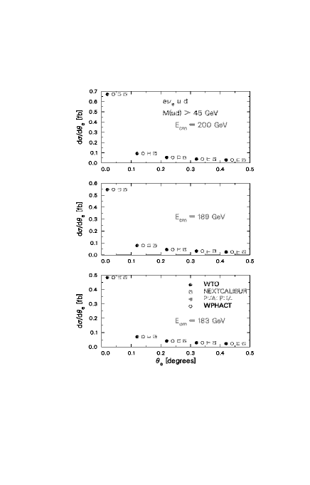
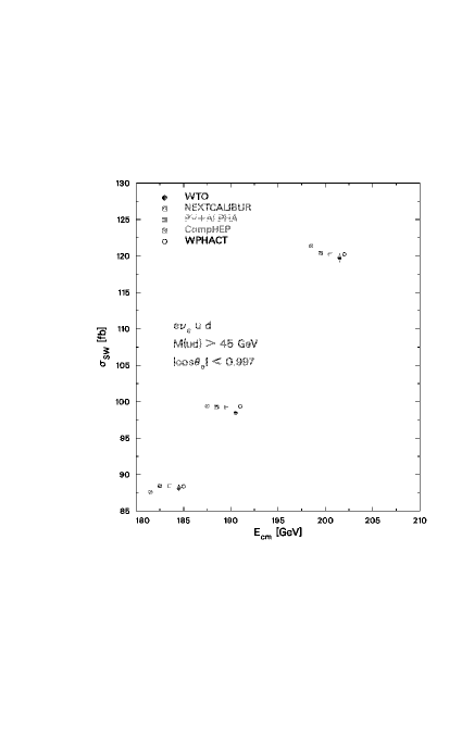
Generally speaking, the technical questions are well under control, both for total cross sections and distributions, as shown by the comparisons in tables 4-5 and figure 6.

As for a realistic modelling of this process, the main difficulties are due to the presence of different scales. Usually, when studying high energy processes, part of the higher order corrections can be reabsorbed in the Born approximation by using the so-called $G_{F}$ scheme. In such a scheme $G_{F}$, $M_{Z}$ and $M_{W}$ are input parameters, while the weak mixing angle and $\alpha_{EM}$ are derived quantities:

$\displaystyle s^{2}_{W}~{}=~{}1-{M^{2}_{W}}/{M^{2}_{Z}}\,,~{}~{}~{}~{}\alpha_{EM}~{}=~{}\sqrt{2}\,\,\frac{G_{F}\,M_{W}^{2}\,s^{2}_{W}}{\pi}\,.$ (2)

In the presence of low $t$-channel scales such an approach fails, since the choice $\alpha(t\sim 0)\sim 1/137$ is certainly more appropriate for the $t$-channel diagrams of figure 4. The question is therefore how to consistently include the running of $\alpha_{EM}$ in single-$W$ four-fermion processes, without breaking gauge invariance.

An exact and field-theoretically consistent solution is represented by the Exact Fermion-Loop (EFL) approach of ref. [17], where the whole, gauge invariant set of fermion one-loop corrections is taken into account, including the vertices.

In table 6 the results of FW and EFL are compared for different cuts on the outgoing electron.

There are also approximate solutions, such as IFLα [18] – where $\alpha(t)$ is used for the $t$-component and $\alpha_{G_{F}}$ for the $s$-component – or the Modified Fermion Loop (MFL) approach by NEXTCALIBUR, that only includes the leading self-energy like corrections from the EFL plus an effective vertex to preserve the $U(1)$ gauge invariance.

IFLα and MFL coincide numerically at LEP2 energies, but slightly disagree with respect to EFL (up to 2% at LEP2). Comparisons at different energies are presented in tables 7 and 8.

\SetScale0.7 \SetWidth1 \SetOffset(80,230) \ArrowLine(50,120)(0,140) \ArrowLine(100,140)(50,120) \ArrowLine(0,0)(50,20) \ArrowLine(50,20)(100,0) \ArrowLine(100,110)(80,70) \ArrowLine(80,70)(100,30) \Photon(50,20)(50,70)27 \Photon(50,70)(50,120)27 \Photon(50,70)(80,70)27 \Text(-14,98)[lc]$e^{+}$\Text(77,98)[lc]$\bar{\nu}_{e}$\Text(-14,0)[lc]$e^{-}$\Text(77,0)[lc]$e^{-}$\Text(77,77)[lc]$\bar{d}$\Text(77,21)[lc]$u$\Text(18,60)[lc]$W$\Text(11,26)[lc]$\gamma,Z$\SetOffset(280,230) \ArrowLine(50,120)(0,140) \ArrowLine(65,126)(50,120) \ArrowLine(100,140)(65,126) \ArrowLine(0,0)(50,20) \ArrowLine(50,20)(100,0) \ArrowLine(100,110)(80,70) \ArrowLine(80,70)(100,30) \Photon(50,20)(50,120)27 \Photon(65,126)(80,70)27 \Text(77,77)[lc]$\bar{d}$\Text(77,21)[lc]$u$\Text(54,76)[lc]$W$\Text(11,66)[lc]$\gamma,Z$\Text(-14,98)[lc]$e^{+}$\Text(77,98)[lc]$\bar{\nu}_{e}$\Text(-14,0)[lc]$e^{-}$\Text(77,0)[lc]$e^{-}$\SetOffset(80,115) \ArrowLine(50,120)(0,140) \ArrowLine(100,140)(50,120) \ArrowLine(0,0)(50,20) \ArrowLine(50,20)(100,0) \ArrowLine(100,110)(80,70) \ArrowLine(80,70)(100,30) \Photon(50,20)(50,120)27 \Photon(18,132)(80,70)27 \Text(77,77)[lc]$\bar{d}$\Text(77,21)[lc]$u$\Text(48,71)[lc]$W$\Text(21,56)[lc]$Z$\Text(-14,98)[lc]$e^{+}$\Text(77,98)[lc]$\bar{\nu}_{e}$\Text(-14,0)[lc]$e^{-}$\Text(77,0)[lc]$e^{-}$\SetOffset(280,115) \ArrowLine(50,120)(0,140) \ArrowLine(100,140)(50,120) \ArrowLine(0,0)(50,20) \ArrowLine(50,20)(100,0) \ArrowLine(100,110)(80,70) \ArrowLine(80,70)(100,30) \Photon(50,20)(50,120)27 \Photon(64,15)(80,70)27 \Text(77,77)[lc]$\bar{d}$\Text(77,21)[lc]$u$\Text(40,41)[lc]$W$\Text(19,56)[lc]$W$\Text(-14,98)[lc]$e^{+}$\Text(77,98)[lc]$\bar{\nu}_{e}$\Text(-14,0)[lc]$e^{-}$\Text(77,0)[lc]$e^{-}$\SetOffset(80,0) \ArrowLine(50,120)(0,140) \ArrowLine(100,140)(50,120) \ArrowLine(0,0)(50,20) \ArrowLine(50,20)(100,0) \ArrowLine(100,90)(50,90) \ArrowLine(50,90)(50,50) \ArrowLine(50,50)(100,50) \Photon(50,20)(50,50)27 \Photon(50,90)(50,120)27 \Text(77,72)[lc]$\bar{d}$\Text(77,26)[lc]$u$\Text(22,52)[lc]$u$\Text(10,20)[lc]$\gamma,Z$\Text(17,77)[lc]$W$\Text(-14,98)[lc]$e^{+}$\Text(77,98)[lc]$\bar{\nu}_{e}$\Text(-14,0)[lc]$e^{-}$\Text(77,0)[lc]$e^{-}$\SetOffset(280,0) \ArrowLine(50,120)(0,140) \ArrowLine(100,140)(50,120) \ArrowLine(0,0)(50,20) \ArrowLine(50,20)(100,0) \ArrowLine(100,90)(50,50) \Line(50,90)(65,78) \ArrowLine(90,58)(100,50) \ArrowLine(50,50)(50,90) \Photon(50,20)(50,50)27 \Photon(50,90)(50,120)27 \Text(77,72)[lc]$\bar{d}$\Text(77,21)[lc]$u$\Text(22,52)[lc]$d$\Text(10,20)[lc]$\gamma,Z$\Text(17,77)[lc]$W$\Text(-14,98)[lc]$e^{+}$\Text(77,98)[lc]$\bar{\nu}_{e}$\Text(-14,0)[lc]$e^{-}$\Text(77,0)[lc]$e^{-}$
Figure 5: $t$-channel diagrams for the $e\nu ud$ single-$W$ final state.
$\sqrt{s}=183\,$GeV $\sqrt{s}=189\,$GeV $\sqrt{s}=200\,$GeV
NEXTCALIBUR $26.483\pm 0.041$ $29.679\pm 0.047$ $35.893\pm 0.048$
SWAP $26.47\pm 0.04$ $29.70\pm 0.04$ $35.93\pm 0.05$
Table 4: Cross-sections [fb] for $e^{+}e^{-}\to e^{-}\bar{\nu}_{e}\mu^{+}\bar{\nu}_{\mu}$.
$\sqrt{s}=183\,$GeV $\sqrt{s}=189\,$GeV $\sqrt{s}=200\,$GeV
NEXTCALIBUR $26.422\pm 0.035$ $29.655\pm 0.046$ $35.954\pm 0.052$
SWAP $26.3\pm 0.2$ $29.6\pm 0.2$ $35.92\pm 0.05$
Table 5: Cross-sections [fb] for $e^{+}e^{-}\to e^{-}\bar{\nu}_{e}\tau^{+}\bar{\nu}_{\tau}$.
Refer to caption
Refer to caption
Figure 6: $\theta_{e}$ distribution and single-$W$ cross sections for $u\bar{d}e^{-}\bar{\nu}_{e}$.
$\theta_{e}\,$[Deg] FW EFL EFL/FW-1 (percent)
$0.0^{\circ}\div 0.1^{\circ}$ 0.14154 0.13448 -4.99
$0.1^{\circ}\div 0.2^{\circ}$ 0.02113 0.02031 -3.88
$0.2^{\circ}\div 0.3^{\circ}$ 0.01238 0.01194 -3.55
$0.3^{\circ}\div 0.4^{\circ}$ 0.00880 0.00851 -3.30
Table 6: $d\sigma/d\theta_{e}$ [pb/degrees], from WTO, for the process $e^{+}e^{-}\to e^{-}\bar{\nu}_{e}\nu_{\mu}\mu^{+}$, for $|\cos\theta_{e}|>0.997$, $E_{\mu}>15\,$GeV, and $|\cos\theta_{\mu}|<0.95$. $\sqrt{s}=183\,$ GeV.
$\sqrt{s}$ FW IFL IFLα EFL EFL/FW-1
(percent)
$183\,{\rm GeV}$ 88.17(44) 88.50(4) 83.26(5) 83.28(6) -5.5(5)
$189\,{\rm GeV}$ 98.45(25) 99.26(4) 93.60(9) 93.79(7) -4.7(3)
$200\,{\rm GeV}$ 119.77(67) 120.43(10) 113.24(8) 113.67(8) -5.1(5)
Table 7: Cross section [fb] for the process $e^{+}e^{-}\to e^{-}\bar{\nu}_{e}u\bar{d}$. $M(u\bar{d})>45\,$GeV, $|\cos\theta_{e}|>0.997$. No ISR.
$\sqrt{s}$ FW IFL IFLα EFL EFL/FW-1
(percent)
$183\,{\rm GeV}$ 26.77(14) 26.45(1) 24.90(1) 25.53(4) -4.6(5)
$189\,{\rm GeV}$ 29.73(14) 29.70(2) 27.98(2) 28.78(4) -3.2(5)
$200\,{\rm GeV}$ 36.45(23) 35.93(4) 33.85(4) 34.97(6) -4.1(6)
Table 8: Cross section [fb] for the process $e^{+}e^{-}\to e^{-}\bar{\nu}_{e}\mu^{+}\nu_{\mu}$. $|\cos\theta_{e}|>0.997$, $E_{\mu}>15\,$GeV, $|\cos\theta_{\mu}|<0.95$. No ISR.

A second problem, relevant when including QED radiation, is the choice of the scales $q^{2}_{i}$ to be used in the Structure Function (SF) formalism, schematically represented in equation (3)

$$d\sigma=\prod_{i}\int dx_{i}\,\,D({q^{2}_{i}},x_{i})~{}d\sigma_{0}\,.$$ (3)

The choice $q^{2}_{i}\sim s$ is proven to reproduce accurately the inclusive four-fermion cross sections, at least for $s$-channel dominated processes. For $t$-channel dominated processes, such as single-$W$ production, a different choice is more adequate, as studies of certain processes have shown. When an exact first order QED radiative correction calculation exists for a $t$-channel dominated process, then the result can be compared to a Structure Function calculation with a $q^{2}$ scale related to the virtuality of the exchanged $t$-channel photon. With such a $q^{2}$ value the two kinds of calculations agree for small angle Bhabha scattering [19] and multi-peripheral two-photon processes [20], where the exact calculation already exists for some time [21]. When no exact first order QED correction calculation is available, the first order soft correction may also serve as a guideline to determine $q^{2}$, as proven by studies performed by GRACE and SWAP [20, 22]. In NEXTCALIBUR, the choice of the scale is performed automatically, event by event, according to the selected final state, as shown in table 9. The final state with 1 $e^{-}$ (or 1 $e^{+}$) is relevant for single-$W$ processes.

Final State $q^{2}_{-}$ $q^{2}_{+}$
No $e^{\pm}$ $s$ $s$
1 $e^{-}$ $|t_{-}|$ $s$
1 $e^{+}$ $s$ $|t_{+}|$
1 $e^{-}$ and 1 $e^{+}$ $|t_{-}|$ $|t_{+}|$
2 $e^{-}$ and 2 $e^{+}$ min($|t_{-}|$) min($|t_{+}|$)
Table 9: The choice of the QED scale in NEXTCALIBUR. $q^{2}_{\pm}$ are the scales of the incoming $e^{\pm}$ while $t_{\pm}$ represent the $t$-channel invariants obtained by combining initial and final state $e^{\pm}$ momenta. When two combinations are possible, as in the last entry of the table, that one with the minimum value of $|t|$ is chosen, event by event.

A further problem is generating a $p_{t}$ spectrum for the photons. Usual solutions are the QED Parton Shower approach (QEDPS) and the use of $p_{t}$ dependent Structure Functions.

For example $p_{t}$ dependent SF are implemented in NEXTCALIBUR via the replacement

$\displaystyle\ln(\frac{q^{2}}{m^{2}_{e}})-1~{}~{}\to~{}~{}\frac{1}{1-c+2\frac{m^{2}_{e}}{q^{2}}}-2\frac{m^{2}_{e}}{q^{2}}\frac{1}{(1-c+2\frac{m^{2}_{e}}{q^{2}})^{2}}$

in the the soft part of the collinear SF, and

$\displaystyle\ln(\frac{q^{2}}{m^{2}_{e}})-1$ $\displaystyle\to$ $\displaystyle\frac{1}{1-c+2\frac{m^{2}_{e}}{q^{2}}}+\frac{1-x}{1+x}\cdot\frac{1}{2}-4\frac{m^{2}_{e}}{q^{2}}\frac{1}{(1+x)(1-c+2\frac{m^{2}_{e}}{q^{2}})^{2}}$

in the hard contributions. After integrating over $c$, one gets $\ln(\frac{q^{2}}{m^{2}_{e}})-1$. The inclusive QED result is therefore recovered and the photon spectrum is exact for small $p_{t}$.

Also GRACE and SWAP implement QEDPS and/or $p_{t}$ dependent SF.

Since $q^{2}=s$ for $s$-channel legs and $q^{2}=|t|$ for $t$-channel dominated legs, the $p_{t}$ distribution is different in the two cases. In order to show this effect, the distribution in $\cos\theta_{\gamma}$ for the most energetic photon (with respect to the incoming $e^{+}$) in $~{}e^{+}e^{-}\to e^{-}\bar{\nu}_{e}u\bar{d}\,(\gamma)$, is shown in figure 7 as predicted by NEXTCALIBUR.

\SetWidth

1 \LinAxis(0,50)(300,50)(10,2,5,0,1.5) \LinAxis(0,250)(300,250)(10,2,-5,0,1.5) \LogAxis(0,50)(0,250)(4,-5,0,1.5) \LogAxis(300,50)(300,250)(4,5,0,1.5) \Text(0 ,40)[t]$-1$\Text(150,40)[t]00\Text(300,40)[t]$1$\Text(-27,100)[l]$10^{-1}$\Text(-27,150)[l]$10^{0}$\Text(-27,200)[l]$10^{1}$\Text(-60,227)[l]$\frac{1}{\sigma}\frac{d\sigma}{d\cos\theta_{\gamma}}$\Text(150,20)[t]$\cos\theta_{\gamma}$\Line( 0.0, 189.7)( 3.0, 189.7) \Line( 3.0, 145.6)( 6.0, 145.6) \Line( 6.0, 135.3)( 9.0, 135.3) \Line( 9.0, 129.3)( 12.0, 129.3) \Line( 12.0, 125.4)( 15.0, 125.4) \Line( 15.0, 119.9)( 18.0, 119.9) \Line( 18.0, 115.5)( 21.0, 115.5) \Line( 21.0, 114.6)( 24.0, 114.6) \Line( 24.0, 110.2)( 27.0, 110.2) \Line( 27.0, 109.4)( 30.0, 109.4) \Line( 30.0, 108.5)( 33.0, 108.5) \Line( 33.0, 107.1)( 36.0, 107.1) \Line( 36.0, 105.6)( 39.0, 105.6) \Line( 39.0, 101.8)( 42.0, 101.8) \Line( 42.0, 102.1)( 45.0, 102.1) \Line( 45.0, 101.1)( 48.0, 101.1) \Line( 48.0, 104.9)( 51.0, 104.9) \Line( 51.0, 98.5)( 54.0, 98.5) \Line( 54.0, 98.2)( 57.0, 98.2) \Line( 57.0, 97.5)( 60.0, 97.5) \Line( 60.0, 94.3)( 63.0, 94.3) \Line( 63.0, 96.3)( 66.0, 96.3) \Line( 66.0, 97.8)( 69.0, 97.8) \Line( 69.0, 98.6)( 72.0, 98.6) \Line( 72.0, 95.3)( 75.0, 95.3) \Line( 75.0, 94.9)( 78.0, 94.9) \Line( 78.0, 94.1)( 81.0, 94.1) \Line( 81.0, 91.8)( 84.0, 91.8) \Line( 84.0, 89.8)( 87.0, 89.8) \Line( 87.0, 91.3)( 90.0, 91.3) \Line( 90.0, 89.3)( 93.0, 89.3) \Line( 93.0, 91.4)( 96.0, 91.4) \Line( 96.0, 87.2)( 99.0, 87.2) \Line( 99.0, 93.5)( 102.0, 93.5) \Line( 102.0, 88.1)( 105.0, 88.1) \Line( 105.0, 88.9)( 108.0, 88.9) \Line( 108.0, 91.7)( 111.0, 91.7) \Line( 111.0, 90.7)( 114.0, 90.7) \Line( 114.0, 90.2)( 117.0, 90.2) \Line( 117.0, 89.6)( 120.0, 89.6) \Line( 120.0, 88.0)( 123.0, 88.0) \Line( 123.0, 85.8)( 126.0, 85.8) \Line( 126.0, 84.3)( 129.0, 84.3) \Line( 129.0, 89.3)( 132.0, 89.3) \Line( 132.0, 89.7)( 135.0, 89.7) \Line( 135.0, 89.6)( 138.0, 89.6) \Line( 138.0, 87.5)( 141.0, 87.5) \Line( 141.0, 91.2)( 144.0, 91.2) \Line( 144.0, 84.7)( 147.0, 84.7) \Line( 147.0, 87.8)( 150.0, 87.8) \Line( 150.0, 89.0)( 153.0, 89.0) \Line( 153.0, 91.0)( 156.0, 91.0) \Line( 156.0, 86.8)( 159.0, 86.8) \Line( 159.0, 88.0)( 162.0, 88.0) \Line( 162.0, 90.2)( 165.0, 90.2) \Line( 165.0, 86.9)( 168.0, 86.9) \Line( 168.0, 87.4)( 171.0, 87.4) \Line( 171.0, 89.9)( 174.0, 89.9) \Line( 174.0, 89.1)( 177.0, 89.1) \Line( 177.0, 89.9)( 180.0, 89.9) \Line( 180.0, 93.0)( 183.0, 93.0) \Line( 183.0, 90.1)( 186.0, 90.1) \Line( 186.0, 90.2)( 189.0, 90.2) \Line( 189.0, 89.6)( 192.0, 89.6) \Line( 192.0, 93.0)( 195.0, 93.0) \Line( 195.0, 88.0)( 198.0, 88.0) \Line( 198.0, 91.5)( 201.0, 91.5) \Line( 201.0, 93.5)( 204.0, 93.5) \Line( 204.0, 93.2)( 207.0, 93.2) \Line( 207.0, 93.3)( 210.0, 93.3) \Line( 210.0, 92.9)( 213.0, 92.9) \Line( 213.0, 92.0)( 216.0, 92.0) \Line( 216.0, 94.4)( 219.0, 94.4) \Line( 219.0, 95.6)( 222.0, 95.6) \Line( 222.0, 96.5)( 225.0, 96.5) \Line( 225.0, 97.0)( 228.0, 97.0) \Line( 228.0, 98.5)( 231.0, 98.5) \Line( 231.0, 94.2)( 234.0, 94.2) \Line( 234.0, 99.7)( 237.0, 99.7) \Line( 237.0, 99.7)( 240.0, 99.7) \Line( 240.0, 100.3)( 243.0, 100.3) \Line( 243.0, 101.4)( 246.0, 101.4) \Line( 246.0, 99.9)( 249.0, 99.9) \Line( 249.0, 102.9)( 252.0, 102.9) \Line( 252.0, 102.5)( 255.0, 102.5) \Line( 255.0, 107.2)( 258.0, 107.2) \Line( 258.0, 106.3)( 261.0, 106.3) \Line( 261.0, 108.3)( 264.0, 108.3) \Line( 264.0, 109.3)( 267.0, 109.3) \Line( 267.0, 111.2)( 270.0, 111.2) \Line( 270.0, 111.5)( 273.0, 111.5) \Line( 273.0, 113.4)( 276.0, 113.4) \Line( 276.0, 115.5)( 279.0, 115.5) \Line( 279.0, 119.0)( 282.0, 119.0) \Line( 282.0, 122.7)( 285.0, 122.7) \Line( 285.0, 126.9)( 288.0, 126.9) \Line( 288.0, 133.3)( 291.0, 133.3) \Line( 291.0, 140.6)( 294.0, 140.6) \Line( 294.0, 150.7)( 297.0, 150.7) \Line( 297.0, 224.4)( 300.0, 224.4) \Line( 3.0, 189.7)( 3.0, 145.6) \Line( 6.0, 145.6)( 6.0, 135.3) \Line( 9.0, 135.3)( 9.0, 129.3) \Line( 12.0, 129.3)( 12.0, 125.4) \Line( 15.0, 125.4)( 15.0, 119.9) \Line( 18.0, 119.9)( 18.0, 115.5) \Line( 21.0, 115.5)( 21.0, 114.6) \Line( 24.0, 114.6)( 24.0, 110.2) \Line( 27.0, 110.2)( 27.0, 109.4) \Line( 30.0, 109.4)( 30.0, 108.5) \Line( 33.0, 108.5)( 33.0, 107.1) \Line( 36.0, 107.1)( 36.0, 105.6) \Line( 39.0, 105.6)( 39.0, 101.8) \Line( 42.0, 101.8)( 42.0, 102.1) \Line( 45.0, 102.1)( 45.0, 101.1) \Line( 48.0, 101.1)( 48.0, 104.9) \Line( 51.0, 104.9)( 51.0, 98.5) \Line( 54.0, 98.5)( 54.0, 98.2) \Line( 57.0, 98.2)( 57.0, 97.5) \Line( 60.0, 97.5)( 60.0, 94.3) \Line( 63.0, 94.3)( 63.0, 96.3) \Line( 66.0, 96.3)( 66.0, 97.8) \Line( 69.0, 97.8)( 69.0, 98.6) \Line( 72.0, 98.6)( 72.0, 95.3) \Line( 75.0, 95.3)( 75.0, 94.9) \Line( 78.0, 94.9)( 78.0, 94.1) \Line( 81.0, 94.1)( 81.0, 91.8) \Line( 84.0, 91.8)( 84.0, 89.8) \Line( 87.0, 89.8)( 87.0, 91.3) \Line( 90.0, 91.3)( 90.0, 89.3) \Line( 93.0, 89.3)( 93.0, 91.4) \Line( 96.0, 91.4)( 96.0, 87.2) \Line( 99.0, 87.2)( 99.0, 93.5) \Line( 102.0, 93.5)( 102.0, 88.1) \Line( 105.0, 88.1)( 105.0, 88.9) \Line( 108.0, 88.9)( 108.0, 91.7) \Line( 111.0, 91.7)( 111.0, 90.7) \Line( 114.0, 90.7)( 114.0, 90.2) \Line( 117.0, 90.2)( 117.0, 89.6) \Line( 120.0, 89.6)( 120.0, 88.0) \Line( 123.0, 88.0)( 123.0, 85.8) \Line( 126.0, 85.8)( 126.0, 84.3) \Line( 129.0, 84.3)( 129.0, 89.3) \Line( 132.0, 89.3)( 132.0, 89.7) \Line( 135.0, 89.7)( 135.0, 89.6) \Line( 138.0, 89.6)( 138.0, 87.5) \Line( 141.0, 87.5)( 141.0, 91.2) \Line( 144.0, 91.2)( 144.0, 84.7) \Line( 147.0, 84.7)( 147.0, 87.8) \Line( 150.0, 87.8)( 150.0, 89.0) \Line( 153.0, 89.0)( 153.0, 91.0) \Line( 156.0, 91.0)( 156.0, 86.8) \Line( 159.0, 86.8)( 159.0, 88.0) \Line( 162.0, 88.0)( 162.0, 90.2) \Line( 165.0, 90.2)( 165.0, 86.9) \Line( 168.0, 86.9)( 168.0, 87.4) \Line( 171.0, 87.4)( 171.0, 89.9) \Line( 174.0, 89.9)( 174.0, 89.1) \Line( 177.0, 89.1)( 177.0, 89.9) \Line( 180.0, 89.9)( 180.0, 93.0) \Line( 183.0, 93.0)( 183.0, 90.1) \Line( 186.0, 90.1)( 186.0, 90.2) \Line( 189.0, 90.2)( 189.0, 89.6) \Line( 192.0, 89.6)( 192.0, 93.0) \Line( 195.0, 93.0)( 195.0, 88.0) \Line( 198.0, 88.0)( 198.0, 91.5) \Line( 201.0, 91.5)( 201.0, 93.5) \Line( 204.0, 93.5)( 204.0, 93.2) \Line( 207.0, 93.2)( 207.0, 93.3) \Line( 210.0, 93.3)( 210.0, 92.9) \Line( 213.0, 92.9)( 213.0, 92.0) \Line( 216.0, 92.0)( 216.0, 94.4) \Line( 219.0, 94.4)( 219.0, 95.6) \Line( 222.0, 95.6)( 222.0, 96.5) \Line( 225.0, 96.5)( 225.0, 97.0) \Line( 228.0, 97.0)( 228.0, 98.5) \Line( 231.0, 98.5)( 231.0, 94.2) \Line( 234.0, 94.2)( 234.0, 99.7) \Line( 237.0, 99.7)( 237.0, 99.7) \Line( 240.0, 99.7)( 240.0, 100.3) \Line( 243.0, 100.3)( 243.0, 101.4) \Line( 246.0, 101.4)( 246.0, 99.9) \Line( 249.0, 99.9)( 249.0, 102.9) \Line( 252.0, 102.9)( 252.0, 102.5) \Line( 255.0, 102.5)( 255.0, 107.2) \Line( 258.0, 107.2)( 258.0, 106.3) \Line( 261.0, 106.3)( 261.0, 108.3) \Line( 264.0, 108.3)( 264.0, 109.3) \Line( 267.0, 109.3)( 267.0, 111.2) \Line( 270.0, 111.2)( 270.0, 111.5) \Line( 273.0, 111.5)( 273.0, 113.4) \Line( 276.0, 113.4)( 276.0, 115.5) \Line( 279.0, 115.5)( 279.0, 119.0) \Line( 282.0, 119.0)( 282.0, 122.7) \Line( 285.0, 122.7)( 285.0, 126.9) \Line( 288.0, 126.9)( 288.0, 133.3) \Line( 291.0, 133.3)( 291.0, 140.6) \Line( 294.0, 140.6)( 294.0, 150.7) \Line( 297.0, 150.7)( 297.0, 224.4)

Figure 7: $\cos\theta_{\gamma}$ distribution for $~{}e^{+}e^{-}\to e^{-}\bar{\nu}_{e}u\bar{d}\,(\gamma)$, by NEXTCALIBUR.

The shape of the distribution can be easily understood in terms of radiation suppression. In fact $|t|\to 0$ implies $D(|t|,x)~{}\sim\delta(1-x)$. Therefore the emission from the incoming $e^{-}$ is suppressed, and the photons are preferably emitted collinearly by the incoming $e^{+}$.

The question of comparing QEDPS and SF has been addressed by the GRACE group. The differences between the two approaches are at the order of 1% for single-$W$ processes. Furthermore, the $E_{\gamma}$ distribution is well reproduced for soft photons, with respect to an exact Matrix Element calculations, while 20% differences are observed (and expected) in the hard region.

In conclusion, putting together all the effects, a theoretical error of 5% 222For semi-leptonic processes this number refers to the High Mass region, namely to situations when appropriate cuts on the jet-jet system are applied in order to suppress the non-perturbative resolved photon contributions. is assigned to single-$W$ processes. This result has to be compared with the accuracy required by the LEP2 collaborations namely 2% for $e^{+}e^{-}\to e^{-}~{}\bar{\nu}_{e}~{}q~{}\bar{q}^{\prime}~{}(\gamma)$, 5% for $e^{+}e^{-}\to e^{-}~{}\bar{\nu}_{e}~{}e^{+}~{}\nu_{e}~{}(\gamma)$, 5% for $e^{+}e^{-}\to e^{-}~{}\bar{\nu}_{e}~{}\mu^{+}~{}\nu_{\mu}~{}(\gamma)$ [1]. However, different pieces of knowledge are still scattered in different codes, and an improvement of the present situation is possible via a multi-step experimental procedure, in which, for example, code A is used to correct code B for the missing effects.

At the LC further improvements are needed. In particular, the genuine EW corrections get larger with increasing energy. Again, a full one-loop four-fermion calculation seems unavoidable, for high precision measurements.

3 Four fermions plus 1 visible photon

This signature gives information on the quartic gauge coupling (see figure 8) and is relevant when studying processes with three final state bosons, such as $W^{+}W^{-}\gamma$ production, $ZZ\gamma$ and $Z\gamma\gamma$. Furthermore, it is a building block for the full computation of $e^{+}e^{-}\to$ 4f at ${\cal O}({\alpha})$.

A bunch of codes contributed, with different strategies. CompHEP, GRACE and HELAC/PHEGAS compute the exact Matrix Element (ME) with massive fermions. RACOONWW uses exact ME, but in the limit of massless fermions. NEXTCALIBUR generates photons only through $p_{t}$ dependent SF. WRAP has a matching between ME and SF generated photons. The last approach allows to estimate the size of the double counting when blindly dressing the $4f+\gamma$ ME with collinear ISR. WRAP observed effects up to 5%, depending on the energy cut used to define the visible photon.

In figure 9 a study by CompHEP is shown on the reliability of a narrow-width approximation.

Distributions generated by GRACE are shown in figure 10.

\SetScale0.7 \SetWidth1 \SetOffset(50,45) \ArrowLine(0,15)(15,-5) \ArrowLine(15,-5)(0,-25) \Photon(15,-5)(30,-5)23 \Photon(40,30)(30,-5)24 \Photon(30,-5)(40,-40)24 \Photon(30,-5)(70,-5)25 \Text(57,-7.5)[l]$\gamma$\Text(14,10)[b]$W^{-}$\Text(14,-20)[t]$W^{+}$\ArrowLine(55,10)(40,30) \ArrowLine(40,30)(55,50) \ArrowLine(40,-40)(55,-20) \ArrowLine(55,-60)(40,-40)
Figure 8: Quartic gauge boson coupling in four-fermion production plus 1 visible $\gamma$.
Refer to caption
Refer to caption
Refer to caption
Refer to caption
Figure 9: Distributions in the $\gamma$ energy, $\gamma$ transverse momentum, $\gamma$ angle with the beam, and in the opening angle between the $\gamma$ and the nearest charged fermion. The distributions for the $e^{+}e^{-}\to\gamma\mu\bar{\nu}_{\mu}u\bar{d}$ are shown by the solid line and the distributions for the $e^{+}e^{-}\to\gamma\mu\bar{\nu}_{\mu}W^{+}$ with the following $W$ isotropic decay are shown by the dashed line.
Refer to caption
Refer to caption
Refer to caption
Refer to caption
Figure 10: $E_{\gamma}$, $\cos\theta_{\gamma}$ and invariant mass distributions for $\mu\nu_{\mu}ud\gamma$.

In tables 10 and 11 the cross sections for inclusive ($\sigma_{\rm tot}$), non radiative ($\sigma_{\rm nrad}$) , single radiative ($\sigma_{\rm srad}$) and double radiative ($\sigma_{\rm drad}$) events are shown, as computed by NEXTCALIBUR. This kind of study is useful for signal definition.

Type Cross-section
$\sigma_{\rm tot}$ 16.107(9)
$\sigma_{\rm nrad}$ 15.018(9)
$\sigma_{\rm srad}$ 1.0697(30)
$\sigma_{\rm drad}$ 0.0189(4)

Table 10: $\sigma$ in fb for $e^{+}(1)e^{-}(2)\to\mu^{-}(3)\mu^{+}(4)u(5)\bar{u}(6)$. $M(34)>10\,$GeV and $M(56)>10\,$GeV. $ZZ$ like cuts, $E_{\gamma}>1\,{\rm GeV},|\cos\theta_{\gamma}|<0.985$.
Type Cross-section
$\sigma_{\rm tot}$ 617.27(59)
$\sigma_{\rm nrad}$ 578.19(58)
$\sigma_{\rm srad}$ 38.54(16)
$\sigma_{\rm drad}$ 0.54(2)

Table 11: $\sigma$ in fb for $e^{+}(1)e^{-}(2)\to\mu^{-}(3)\bar{\nu}_{\mu}(4)u(5)\bar{d}(6)$. $M(56)>10\,$GeV. $WW$ like cuts, $E_{\gamma}>1\,{\rm GeV},|\cos\theta_{\gamma}|<0.985$.

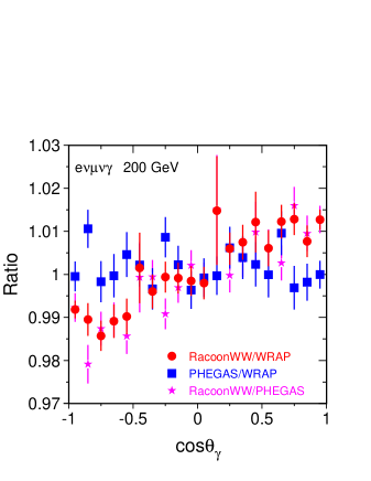
Finally, in table 12 and figure 11, I show results of tuned comparisons among HELAC/PHEGAS, RACOONWW and WRAP.

Process WRAP RacoonWW PHEGAS/HELAC
$u\bar{d}\mu^{-}\bar{\nu}_{\mu}\gamma$ 75.732(22) 75.647(44) 75.683(66)
$u\bar{d}e^{-}\bar{\nu}_{e}\gamma$ 78.249(43) 78.224(47) 78.186(76)
$\nu_{\mu}\mu^{+}\tau^{-}\bar{\nu}_{\tau}\gamma$ 28.263(9) 28.266(17) 28.296(22)
$\nu_{\mu}\mu^{+}e^{-}\bar{\nu}_{e}\gamma$ 29.304(19) 29.276(17) 29.309(25)
$u\bar{d}s\bar{c}\gamma$ 199.63(10) 199.60(11) 199.75(16)
Table 12: $\sigma$ in fb from WRAP, RacoonWW and PHEGAS/HELAC.
Refer to caption
Refer to caption
Figure 11: $\cos\theta_{\gamma}$ distributions and ratios for $\nu_{\mu}\mu^{+}e^{-}\bar{\nu}_{e}\gamma$.
channel YFSZZ ZZTO $G_{F}$-scheme ZZTO $\alpha$-scheme
$qqqq$ 294.6794(490) 298.4411(60) 294.5715(59)
$qq\nu\nu$ 175.4404(302) 175.5622(35) 174.9855(35)
$qq{\rm ll}$ 88.1805(134) 88.7146(18) 87.9881(18)
${\rm ll}\nu\nu$ 26.2530(463) 26.0940(5) 26.1342(5)
${\rm llll}$ 6.5983(15) 6.5929(1) 6.5706(1)
$\nu\nu\nu\nu$ 26.1080(71) 25.8192(5) 25.9868(5)
total 617.2596(755) 621.2241(124) 616.2366(123)
Table 13: $ZZ$ cross-section [fb] at $\sqrt{s}=188.6\,$GeV. YFS exponentiation is used by YFSZZ, while ZZTO includes EFL corrections in the $\alpha$-scheme.

In conclusion, a very good technical precision has been reached in the computation of four-fermion processes plus 1 additional photon. However, the non-logarithmic ${\cal O}(\alpha)$ corrections are not known. Therefore a 2.5% theoretical accuracy on total cross section and inclusive distributions is estimated at LEP2 energies [1]. Larger effects are expected at the LC.

4 $Z$-pair production

Less accuracy is required at LEP2 for this observable with respect to the $W$-pair case. Thought feasible in principle, a DPA $ZZ$ calculation is not available yet. A theoretical accuracy of 2% on $\sigma_{ZZ}$ is estimated at LEP2 by varying the renormalization scheme and by comparing different codes and different treatments of the QED radiation (see table 13).

5 Conclusions

Four-fermion Physics at LEP2 is in a good shape. Thanks to the results of ref. [1], improved calculations are available for

  • $W$-pair production

  • Single-$W$ production

  • Four fermions plus 1 visible $\gamma$

  • $Z$-pair production.

In general, the theoretical accuracies required by the LEP2 experiments are achieved.

At the LC more accuracy is needed. In particular radiative corrections must be included.

Four-fermion loop calculations at ${\cal O}(\alpha_{s})$ already exist [23], while a full ${\cal O}(\alpha)$ EW calculation is still missing.

References

  • [1] M. W. Grünewald et al., in Reports of the working groups on precision calculations for LEP2 Physics, CERN 2000-009 (2000), eds. S. Jadach, G. Passarino and R. Pittau, p. 1, hep–ph/0005309.
  • [2] W. Beenakker, F. A. Berends and A. P. Chapovsky, Nucl. Phys. B548 (1999) 3.
  • [3] E. Boos, M. Dubinin, V. Ilyin, A. Pukhov and V. Savrin, preprint INP MSU 94-36/358, 1994 (hep–ph/9503280);
    P. Baikov et.al, in: Proc. of X Workshop on High Energy Physics and Quantum Field Theory, ed. by B. Levtchenko, V. Savrin, Moscow, 1996, p.101;
    A. Pukhov et.al., hep–ph/9908288;
    see also http://theory.npi.msu.su/~comphep.
  • [4] D. Bardin, J. Biebel, D. Lehner, A. Leike, A. Olchevski and T. Riemann Comp. Phys. Commun. 104 (1997) 161.
  • [5] T. Ishikawa, T. Kaneko, K. Kato, S. Kawabata, Y. Shimizu and H. Tanaka, KEK Report 92-19, 1993, The GRACE manual Ver. 1.0.
    See also H. Tanaka, Comp. Phys. Commun. 58 (1990) 153,
    H. Tanaka, T. Kaneko and Y. Shimizu, Comp. Phys. Commun. 64 (1991) 149.
  • [6] S. Jadach, W. Płaczek, M. Skrzypek, B.F.L. Ward and Z. Wa̧s, Comp. Phys. Commun. 119 (1999) 272.
  • [7] F. A. Berends, C. G. Papadopoulos and R. Pittau, hep-ph/0002249 and hep-ph/0011031.
  • [8] A. Kanaki and C. G. Papadopoulos, Comp. Phys. Commun. 132 (2000) 306, hep–ph/0007335 and hep–ph/0012004.
  • [9] A  Denner, S. Dittmaier, M. Roth and D. Wackeroth, Nucl. Phys. B560 (1999) 33, Phys. Lett. B475 (2000) 127 and hep–ph/9912447.
  • [10] Based on the algorithm by F. Caravaglios and M. Moretti, Phys. Lett. B358 (1995) 332.
    See also G. Montagna, O. Nicrosini, F. Piccinini, Comp. Phys. Commun. 98 (1996) 206;
    G. Montagna, M. Moretti, O. Nicrosini, F. Piccinini, Nucl. Phys. B541 (1999) 31;
    G. Montagna, M. Moretti, O. Nicrosini, A. Pallavicini and F. Piccinini, hep–ph/0005121.
  • [11] E. Accomando and A. Ballestrero, Comp. Phys. Commun. 99 (1997) 270.
  • [12] G. Passarino, Comp. Phys. Commun. 97 (1996) 261
  • [13] S. Jadach, W. Płaczek and B. F. L. Ward, Phys. Rev. D56 (1997) 6939.
  • [14] G. Passarino, http://www.to.infn.it/~giampier/zzto.
  • [15] R. G. Stuart, Phys. Lett. B262 (1991) 113;
    A. Aeppli, G. J. van Oldenborgh and D. Wyler, Nucl. Phys. B428 (1994) 126;
    W. Beenakker, F. A. Berends and A. P. Chapovsky, Nucl. Phys. B548 (1999) 3;
    A. Denner, S. Dittmaier and M. Roth, Nucl. Phys. B519 (1998) 39.
  • [16] D. Bardin et al., Report on Event Generators for WW Physics in Vol.1, Report of the Workshop in Physics at LEP2, Altarelli, G. et al., eds., 1996, CERN-96-01;
    E. N. Argyres et al., Phys. Lett. B358 (1995) 339.
  • [17] G. Passarino, Nucl. Phys. B574 (2000) 451 and Nucl. Phys. B578 (2000) 3.
    See also W. Beenakker et al., Nucl. Phys. B500 (1997) 255 and ref. [16].
  • [18] See the contribution by WPHACT to ref. [1], and E. Accomando, A. Ballestrero and E. Maina, Phys. Lett. B479 (2000) 209.
  • [19] W. Beenakker, F. A. Berends and S. C. van der Marck, Nucl. Phys. B359 (1991) 323.
  • [20] Y. Kurihara, J. Fujimoto, Y. Shimizu, K. Kato, K. Tobimatsu and T. Munehisa, Prog. Theor. Phys.  103 (2000) 1199.
  • [21] F. A. Berends, P. H. Daverveldt and R. Kleiss, Nucl. Phys. B253 (1985) 421.
  • [22] G. Montagna, M. Moretti, O. Nicrosini, A. Pallavicini and F. Piccinini, hep–ph/0005121.
  • [23] E. Maina, R. Pittau and M. Pizzio Phys. Lett. B429 (1998) 354, Phys. Lett. B393 (1997) 445 and hep–ph/9709454.